Type-1.5 superconductivity in muliband and other multicomponent systems
Abstract
Usual superconductors are classified into two categories as follows: type-1 when the ratio of the magnetic field penetration length () to coherence length () and type-2 when . The boundary case is also considered to be a special situation, frequently termed as “Bogomolnyi limit”. Here we discuss multicomponent systems which can possess three or more fundamental length scales and allow a separate superconducting state, which was recently termed “type-1.5”. In that state a system has the following hierarchy of coherence and penetration lengths . We also briefly overview the works on single-component regime and comment on recent discussion by Brandt and Das in the proceedings of the previous conference in this series. Prepared for the proceedings of International Conference on Superconductivity and Magnetism 2012
I Introduction
I.0.1 Type-1, type-2 and type-1.5 superconductivity.
The fundamental classification of superconductors is based on the their description in terms of the classical field theory: the Ginzburg-Landau (GL) model, and the fundamental length scales which it yields: the coherence length and the magnetic field penetration length . There type-1 and type-2 regimes can be distinguished in many ways, through magnetic response, properties and stability of topological defects, orders of the phase transitions etc.
Type-1 superconductors expel weak magnetic fields, by generating surface currents. In stronger fields finite-size samples form non-universal configuration of macroscopic normal domains with magnetic flux [1, 2, 3]. The supercurrent in that case flows both on the surface and near the boundaries of these domains. The response of type-2 superconductors is different [4]; below some critical value , the field is expelled. Above this value a superconductor forms a lattice or a liquid of vortices which carry magnetic flux through the system. Since vortices are formed by the supercurrent it also implies that type-2 superconductor in external field allow current configuration in its bulk (in contrast to only surface currents in type-1 case). Only at a higher second critical value, superconductivity is destroyed.
The special “zero measure” boundary case where has a critical value exactly at the type-1/type-2 boundary is legitimately distinguished as a separate case (frequently called “Bogomolnyi regime”). In the most common GL model parameterization it corresponds to . In that case stable vortex excitations exist but they do not interact [5, 6] in the Ginzburg-Landau theory. This regime is a subject of quite broad interest also beyond condensed matter context [7].
It was recently shown that in multicomponent systems systems (in particular in multiband superconductors) there is a regime which falls outside the type-1/type-2 dichotomy [8, 9, 10, 11, 14, 12, 13, 18, 17, 19, 15, 16, 20], see also recent related works [21, 22, 23, 24, 25] In that case the system possesses two or more coherence lengths such that (in the most general N-component case) and there are thermodynamically stable vortices with long-range attractive, short range repulsive interaction, as a consequence of this hierarchy of length scales. Owing to its multicomponent nature there are two kinds of superflows in the system and they can have coexisting type-1 and type-2 tendencies, and do not fall exclusively under the definitions of either type-1 or type-2 cases.
I.0.2 Bogomolnyi regime
Let us start by making some remarks about a particular limit of single component Ginzburg-Landau theory: the Bogomolnyi regime . It is a property of Ginzburg-Landau model where, at , the core-core attractive interaction between vortices exactly cancels the current-current repulsive interaction at all distances as was first discussed by Kramer and later in more detail by Bogomolnyi [5, 6]. For a review of current studies of that regime in the Ginzbug-Landau theory see [7]. However indeed in a realistic system even in the limit , there will be always leftover inter-vortex interactions, (appearing beyond the GL field theoretic description), form underlying microscopic physics. The form of that interaction potential is determined not by the fundamental length scales of the GL theory but by non-universal microscopic physics and in general it can indeed be non-monotonic.
The idea of searching for non-monotonic intervortex potential from microscopic corrections in the Bogomolnyi regime was suggested by Eilenberger and Buttner [26], and later by Halbritter, Dichtel [26] [27, 28]. Unfortunately, as was later discussed by b Leung and Jacobs these early works were based on uncontrollable approximations[32, 33]. Nonetheless the importance of Eilenberger’s work cannot be denied as it appears to be the first to raise the question if the cancellation of intervortex interaction forces in the Ginzburg-Landau model with can give raise to the extretemely weak but qualitatively interesting microscopic-physics dominated intervortex forces. It should be noted that all of the above works do not discuss universal physics, but are focused on specific microscopic physics of a weakly coupled BCS superconductor.
II Type-1.5 superconductors
In this paper we focus on what kind of new physics can arise in multicomponent superconductors. We argue that type-1/type-2 dichotomy breaks down in these systems despite various couplings between the components.
The Ginzburg-Landau free energy functional for multicomponent system has the form
| (1) |
Here are complex superconducting components, , and , , and stands for effective potential. Depending on symmetry of the system there can also be present mixed (with respect to components ) gradient terms (for a more detailed review see [10, 17]).
The main situations where multiple superconducting components arise are (i) multiband superconductors [34, 35, 36, 37, 38, 39, 40, 41, 42, 43, 44] (where represent condensates belonging to different bands), (ii) mixtures of independently conserved condensates such as the projected superconductivity in metallic hydrogen and hydrogen rich alloys [45, 46, 47, 48, 49], (where represent electronic and protonic Cooper pairs or deuteronic condensate) or models of nuclear superconductors in neutron stars interior [50] (where represent protonic and hyperonic condensates) and (iii) superconductors with nontrivial pairing symmetries. The principal difference between the cases (i) and (ii) is the absence of the intercomponent Josephson coupling in case of system like metallic hydrogen (ii) because there the condensates are independently conserved. Thus the symmetry is or higher. In the case (i) multiple superconducting components originate from Cooper pairing in different bands. Because condensates in different bands are not independently conserved there is a rather generic presence of intercomponent Josephson coupling in that case.
II.1 Type-1.5 superconductivity
The possibility of a new type of superconductivity, distinct from the type-1 and type-2 [8, 9, 10, 11, 12, 13, 14] comes from the following considerations. As discussed in [8, 9, 10, 11, 12, 13, 14], the two-component models in general are characterized by three fundamental length scales: magnetic field penetration length and two coherence lengths which renders the model impossible to parameterize in terms of a single dimensionless parameter and thus the type-1/type-2 dichotomy is not sufficient for classification. Rather, in a wide range of parameters, as a consequence of the existence of three fundamental length scales, there is a separate superconducting regime with . In that regime as a consequence of coexisting type-1 and type-2 tendencies the following situation is possible: vortices can have long-range attractive (due to “outer cores” overlap) and short-range repulsive interaction (driven by current-current and electromagnetic interaction) and form vortex clusters immersed in domains of two-component Meissner state [8, 9]. It should be noted that the non-monotonic intervortex interaction is one of the necessary properties of type-1.5 regime but is not a defining property (more details of it is given below, see also [17]). Here we summarize the basic properties of type-1, type-2 and type-1.5 regimes in the table 1 [10]. Recent experimental works [11, 18] proposed that this state is realized in the two-band material MgB2. In Ref. [11] this regime was termed “type-1.5” superconductivity by Moshchalkov et al. These works resulted in increasing interest in the subject [21, 19, 22, 24, 25]. Recently a counterpart of type-1.5 regime was discussed in context of quantum Hall effect [51].
If the vortices form clusters one cannot use the usual one-dimensional argument concerning the energy of superconductor-to-normal state boundary to classify the magnetic response of the system. First of all, the energy per vortex in such a case depends on whether a vortex is placed in a cluster or not. Formation of a single isolated vortex might be energetically unfavorable, while formation of vortex clusters is favorable, because in a cluster where vortices are placed in a minimum of the interaction potential, the energy per flux quantum is smaller than that for an isolated vortex. Also the boundary conditions for magnetic field do not involve having at () and thermodynamical critical field values at () . Furthermore, besides the energy of a vortex in a cluster, there appears an additional energy characteristic associated with the boundary of a cluster but in general that boundary energy also depends on structure and size of a cluster. So in that case the argument of the boundary energy is not a useful characteristic since there are there are many different solutions for different interfaces, some of which have negative energy while others (such as the energy of a vortex cluster boundary) have positive energy.
| single-component Type-1 | single-component Type-2 | multi-component Type-1.5 | |
|---|---|---|---|
| Characteristic lengths scales | Penetration length & coherence length () | Penetration length & coherence length () | Two characteristic density variations length scales , and penetration length , the non-monotonic vortex interaction occurs in these systems in a large range of parameters when |
| Intervortex interaction | Attractive | Repulsive | Attractive at long range and repulsive at short range |
| Energy of superconducting/normal state boundary | Positive | Negative | Under quite general conditions negative energy of superconductor/normal interface inside a vortex cluster but positive energy of the vortex cluster’s boundary |
| The magnetic field required to form a vortex | Larger than the thermodynamical critical magnetic field | Smaller than thermodynamical critical magnetic field | In different cases either (i) smaller than the thermodynamical critical magnetic field or (ii) larger than critical magnetic field for single vortex but smaller than critical magnetic field for a vortex cluster of a certain critical size |
| Phases in external magnetic field | (i) Meissner state at low fields; (ii) Macroscopically large normal domains at larger fields. First order phase transition between superconducting (Meissner) and normal states | (i) Meissner state at low fields, (ii) vortex lattices/liquids at larger fields. Second order phase transitions between Meissner and vortex states and between vortex and normal states at the level of mean-field theory. | (i) Meissner state at low fields (ii) “Semi-Meissner state”: vortex clusters coexisting with Meissner domains at intermediate fields (iii) Vortex lattices/liquids at larger fields. Vortices form via a first order phase transition. The transition from vortex states to normal state is second order. |
| Energy E(N) of N-quantum axially symmetric vortex solutions | for all N. Vortices collapse onto a single N-quantum mega-vortex | for all N. N-quantum vortex decays into N infinitely separated single-quantum vortices | There is a characteristic number Nc such that for N Nc, while for N Nc. N-quantum vortices decay into vortex clusters. |

III Length scales and type-1.5 regime in two-band Ginzburg-Landau Model with arbitrary interband interactions.
Type-1.5 regimes with has a clear interpretation in superconductors, which is the simplest example of a superconductor which cannot be parameterized by Ginzburg-Landau parameter . Here we overview how coherence length are defined in Ginzburg-Landau model for two-band superconductors. These systems have non-zero interband interactions. Consider the most general GL model for two-band superconductors
| (2) |
Here , and , , represent two superconducting components which, in a two-band superconductor are associated with two different bands. Ref. 9 discussed how coherence lengths are modified by interband Josephson coupling. In Ref. 10 the analysis was carried out for a GL model with arbitrary interband interactions. Here we briefly reproduce the key aspects of the analysis from Refs. 10, 17. In this analysis we allow the term to contain an arbitrary collection of non-gradient terms representing various inter and intra-band interactions. I.e. includes but is not limited to interband Josephson coupling Below we show how three characteristic length scales are defined in this two component model (two are coherence lengths, associated with densities variations and the London magnetic field penetration length), yielding type-1.5 regime . Note that existence of two bands in a superconductor is not a sufficient conditions for a superconductor to be described by a two-component Ginzburg-Landau model. Conditions of appearance of regimes when the system does not allow a description in terms of two-component fields theory (2) is discussed in the work based on microscopic considerations in Refs. [12, 13]. However for a wide parameter range two-component GL expansions are justfied on formal grounds [13]
The effect of mixed gradient terms (which in this system are induced by interband impurity scattering) was studied in [10]. Below we consider the clean limit, thus we have to set , a reader interested in the effects of these term can check the Ref [10]. The Josephson coupling which is contained in tends to lock phase difference to or depending on sign of . Lets denote the ground state values of fields as where and . To define coherence lengths one has to consider small deviations of the field around ground state values (, ) and linearize the model in small deviations around the ground state (here we consider that the phases are locked by Josephson coupling )
| (3) |
Here, is the Hessian matrix of about , that is,
| (4) |
Now in , the vector potential decouples and yields the London magnetic field penetration length
| (5) |
In contrast, when there is interband coupling the density fields are, in general, coupled (i.e. in general the symmetric matrix has off-diagonal terms). To be able to define coherence lengths that coupling should be removed by a linear redefinition of fields [9, 10, 17],
| (6) |
Then the linear theory decouples and thus allow to define two distinct coherence lengths
| (7) |
Thus the interband coupling, such as the Josephson terms introduces hybridization of the fields. The new coherence lengths are associated not with the fields but with their linear combinations
| (8) |
| (9) |
IV Vortex clusters in a Semi-Meissner state. Numerical results
In this section, following Ref. [14] we overview numerical solution for vortex clusters in two-component Ginzburg-Landau model
| (10) |
Here again, , and . Figure 2 (from Ref. [14]) shows numerical solution for vortex cluster in type-1.5 superconductor with symmetry. The cases where symmetry is weakly broken by interband Josephson coupling are qualitatively similar [14].

From this numerical solution one can clearly see the hallmark of type-1.5 superconductivity: the coexisting and competing type-1 and type-2 behaviors of the condensates despite their electromagnetic coupling. Here the second component has a type-1 like behavior, essentially its current is concentrated on the surface of a vortex cluster similarly like current on a surface of a type-1 superconductor, or on boundary of macroscopic normal domains. On the contrary the first component tends to from well separated vortices.
V Discussion and Reply to Brandt and Das [52].
In the proceedings of the previous conference of this series, E.H. Brandt and M. Das [52] criticized the idea of type-1.5 superconductivity. In this section we discuss that these objections are incorrect and point out that also unfortunately their overview of this idea and literature is highly inaccurate. Also we discuss that the following speculations in [52] are unfortunately incorrect: namely after dismissing the possibility of type-1.5 superconductivity in two-band systems, the authors of [52] put forward a conjecture that intervortex attraction reported by Moshchalkov et al [11] might still be possible in but via some unrelated microscopic mechanisms like those which give intervortex attraction in single-component systems with . As we point out below these mechanisms cannot lead to intervortex attraction in superconductors like where the condition does not hold.
First we would like to add some remarks on the single-component regime in single-component systems and to mention some references on pioneering works and works of key importance, none of which unfortunately were cited in Ref.52. The idea of possible non-monotonic intervortex potential in single-component models from microscopic corrections (when the attractive and repusilve parts of forces at the GL-theory level cancel each other out) was first suggested by Eilenberger and Buttner [26], Halbritter [27] and Dichtel [28]. We stress that Brandt also should be credited for being one of the first who followed up on these ideas, more precisely on the work by Dichtel [29]. However, as discussed by Leung and Jacobs the mechanism suggested by all the listed above early works, was unfortunately unrelated to the physics of long-range vortex attraction in superconductors with [32]. There was also a rather early works by Jacobs [30] who was searching for intervortex attraction in superconductors with by generalized the work of Neumann and Tewordt [31]. The question that in weak-coupling superconductors with , microscopic corrections can lead to intervortex attraction was put on more solid grounds in the important work by Jacobs and Leung [32, 33].
In the review of experiments on single component materials with the Ref. [52] reports two figures (Figs. 3 and 4 in [52]) which are interpreted therein as experimental evidence for attractive intervortex forces in Nb. However unfortunately these figures show evidence that actually an opposite effect takes place: namely they suggest that long-range intervortex forces are repulsive. Indeed the vortex clusters in Fig. 4 form nearly hexagonal structure, which is only possible in the systems with long-range repulsive interaction. Such vortex arrangements are impossible if long-range interaction were attractive. The Figs. 3 and 4 in Ref.52 show stripe and clump phases which are known to occur in systems with two-scale purely repulsive interactions [53]. Indeed the additional repulsive tail in the intervortex interaction can arise because of intervortex interaction via stray magnetic fields above the surface of a sample[54] (in fact the possibility that repulsive forces due to stray fields play role in vortex structure formation in these experiments was already discussed by Kramer [5]). Therefore the images cited in [52] do not present evidence for vortex attraction in Nb, but rather present evidence to the contrary. A good review of current theoretical and experimental evidence which is in favor of intervortex attraction in Nb can be found in the book by Huebener [55].
From a theoretical viewpoint the possibility of attractive intervortex interaction for weak-coupling superconductors with is quite well established. However the conjecture that this physics might somehow be relevant for systems like is certainly incorrect. Namely, in these theories, in single-component case one cannot get any appreciable intervortex attraction through these mechanisms for . This is because, this mechanism is based on cancellation of forces at the level of Ginzburg-Landau theory when . Introducing any, even small coupling to a second band in general rapidly shrinks the parameter space where a system can have a regime analogous to Bogomolnyi limit (). In case of multiple bands, achieving the Bogomolnyi limit requires a fine tuning of GL parameters. That is, in general multicomponent systems, in general, the region where GL interactions are canceled out has zero measure for all practical purposes. In brief going to multicomponent system does not enhance the physics of Bogomolnyi point () but instead dramatically shrinks the parameter space where this physics can occur.
The Bogomolnyi regime is indeed principally different from type-1.5 superconductivity. In type-1.5 regime the non-monotonic interaction forces is the consequence of the existence of several superconducting components with several coherence lengths such that . The physics of type-1.5 regime is all about the coexistence of components with type-1 and type-2 tendencies which is not possible in single component system.
Lets us also reply to the arguments, based on which the authors of Ref.52 dismissed the possibility of type-1.5 superconductivity. They summarized their argument as In brief, mixing two components as visualized by Babaev et al. and Moshchalkov et al., will not produce a new kind of superconductivity, because in the mixture (magnetic field penetration length) is determined self-consistently. Also Ref.52 criticizes works on type-1.5 superconductivity by claiming that these works considered only the limit of zero interband coupling between the superconducting components from different bands. Ref.52 also questioned whether two coherence length can be defined in multiband superconductors, namely: It is shown that for the real superconductor which possesses a single transition temperature, the assumption of two independent order parameters with separate penetration depths and separate coherence lengths is unphysical.
Unfortunately all of these statements are factually not correct. First, none of the papers on type-1.5 superconductivity ever attributed different penetration lengths to different bands (notations were used merely to parametrize Ginzbgurg-Landau model, as was very explicitly stated in [8]). Perhaps the origin of that misunderstanding can be traced to a simple misconception of what constitutes intercomponent electromagnetic coupling, reflected in the statements in Sections 4 and 7 in 52. Namely it is stated there that the terms represent “electromagnetic coupling between the condensates”. Unfortunately it is not correct because these terms are mixed gradient terms. The physical origin of these terms in two-band supercondctors is multiband impurity scattering [37, 39] and thus they have little to do with electromagnetic coupling. Moreover even when such terms are present, in general they do not eliminate type-1.5 regime [10]. In contrast the electromagnetic coupling is entirely mediated by the vector potential and does not require any mixed gradient terms. In fact in the Ref.8 it was discussed in considerable detail how penetration length is determined self-consistently.
Next the Ref. 52 criticizes the work Ref.8 for “neglecting” interband Josephson coupling and claims that this coupling is “generic”. However first we should note that this coupling is not generic and in some systems it is in fact forbidden on symmetry grounds (corresponding references, on the systems where such situations occur were given in Ref. 8, 10). Second, we should remark that for the system where Josephson coupling is present, its effects on type-1.5 regime was addressed [9] long before the appearance of Ref. 52, where this paper was not referenced. More recent papers studied effects of this coupling in more detail [10, 12, 13] and as reviewed here indeed it does not eliminate the type-1.5 regime.
The statement that in the presence of interband coupling one cannot define two coherence lengths is a more common misconception, also shared by other groups [56]. For example the authors of Ref. [56] came to such a conclusion after a failed attempt [57] to attribute different coherence lengths directly to different gap fields neglecting hybridization. This naive approach is indeed technically incorrect (see the Comment Ref. 58). As discussed above, two coherence length are well defined when one takes into account hybridization: i.e. when one attributes coherence lengths to different linear combinations of the gap fields[9, 10, 12, 13, 17]. Also as reviewed below two-component GL expansion is well justified on formal grounds under certain conditions even when interband coupling is present [13].
The statement about non-existence of two order parameters in the abstract of Ref.52 is indeed entirely irrelevant for the existence of type-1.5 regime. Note that in our works on two-band systems [9, 10, 12, 13, 17] were did not call “order parameters”, although this misnomer terminology is very commonly accepted recently. In two-band system symmetry is explicitly broken to local symmetry. Thus indeed the order parameter is a single complex field. However, in general, the number of components in the effective field theory (such as Ginzburg-Landau theory) has nothing to do with the notion of order parameters. The number of components in GL theory is only related to question whether or not the system is described by a multicomponent classical effective field theory in some regime. One can have a perfectly valid description of a system in terms of Ginzburg-Landau or Gross-Pitaevskii complex fields theory even when there are no order parameters at all and no spontaneously broken symmetries. The simplest examples are two-dimensional systems at finite temperature (where indeed cannot be called an order parameter), a different example is superfluid turbulence. Similarly in two-band case the system can have entirely well justified description in terms of two-component GL theory with two distinct coherence lengths, despite having only symmetry and thus only a single order parameter [13].
To summarize this part: the physics of the regime has unfortunately no relationship to type-1.5 superconductivity, which occurs in multicomponent systems when . Also long-range vortex attraction is necessary for type-1.5 regime but is not its defining property (type-1.5 regime requires at least two superconducting components). Finally two-component GL field theory and two coherence lengths are well defined in case of interacting bands. In the next section we review the recently published microscopic theory of the type-1.5 regime [12, 13], from which is it also quite apparent that this physics is principally different from the physics of Bogomolnyi point ( in single-component theory).
VI Microscopic theory of type-1.5 superconductivity
The phenomenological Ginzburg-Landau model described above predicts the possibility of 1.5 superconducting state. This form of two-component Ginzburg-Landau expansion was microscopically justified on formal grounds [13]. Strictly speaking the GL theory is justified only at elevated temperatures. To describe type-1.5 superconductivity in all temperature regimes (except, indeed the region where mean-field theory is inapplicable) as well as to make a quantitative connection with a certain class of the real systems requires a microscopic approach which also does not rely on a GL expansion. The described above physics of type-1.5 regime was recently justified by self-consistent Eilenberger theory [12]. We consider a superconductor with two overlapping bands at the Fermi level [34]. The corresponding two sheets of the Fermi surface are assumed to be cylindrical. Within quasi-classical approximation the band parameters characterizing the two different sheets of the Fermi surface are the Fermi velocities and the partial densities of states (DOS) , labelled by the band index and parameterized by BCS pairing constants (intraband) and (interband).
The asymptotic of the gap functions in two superconducting bands at distances far from the vortex core can be found by linearizing the Eilenberger equations together with the self-consistency equations. The asymptotic of the linearized system is governed by the complex plane singularities of response function found in Ref.(12) among which are the poles and branch cuts. In general there are two regimes regulating the asymptotic behavior of gap functions. The first regime is realized when two poles of the response function lie below the branch cut. The two poles determine the two coherence lengths or, equivalently, the two masses of composite gap functions fields (i.e. linear combinations of the fields as in the previous section), which we denote as “heavy” and “light” (i.e. ). This is principally different from microscopic theories of the single-component regime. At elevated temperatures these masses (or inverse coherence lengths) are exactly the same as the given by a corresponding two-component GL theory obtained by the gradient expansion from the microscopic theory [13]. The GL theory under certain conditions can be also used at relatively low temperatures [13].
The second regime is realized at lower temperatures when there is only one pole of the response function lying below the branch cut in the complex plane. In this case the asymptotic is determined by the light mass mode and the contribution of the branch cut which has all the length scales smaller than some threshold one determined by the position of the lowest branch cut on the imaginary axis. The branch cut contribution is essentially non-local effect which is not captured by GL theory therefore one can expect growing discrepancies between effective GL solution and the result of microscopic theory at low temperatures.
The examples from Ref. 12 of the temperature dependencies of the inverse coherence lengths are shown in the Fig.3. The evolution of the inverse coherence lengths is shown in the sequence of plots Fig.3(a)-(d) for increasing from the small values to the values comparable to intraband coupling . The two massive modes coexist at the temperature interval , where the temperature is determined by the branch cut position, shown in the Fig.3 by black dashed line. For temperatures there exists only one mode and as the interband coupling parameter is increased, the temperature rises and becomes equal to at some critical value of .
As shown on Fig.3a,b the function is non-monotonic at low temperatures. The temperature dependence of the inverse coherence length has anomalous behavior[12], which is in strong contrast to temperature dependence of the mass of the gap mode in single-band theories.

To assess the effect of non-monotonic temperature dependence of inverse coherence length on the vortex structures in two-band superconductors we calculated self-consistently [12, 13] the structure of isolated vortex for different values of . A complex aspect of the vortex structure in two-band system is that in general the exponential law of the asymptotic behavior of the gaps is not directly related to the “core size” at which gaps recover most of their ground state values. We can characterize this effect by defining a “healing” length of the gap function as follows . The characteristic example of the vortex structure is shown in Fig. 4a. For this case we obtain that for all values of . On the contrary, the healing length of changes significantly such that for correspondingly.
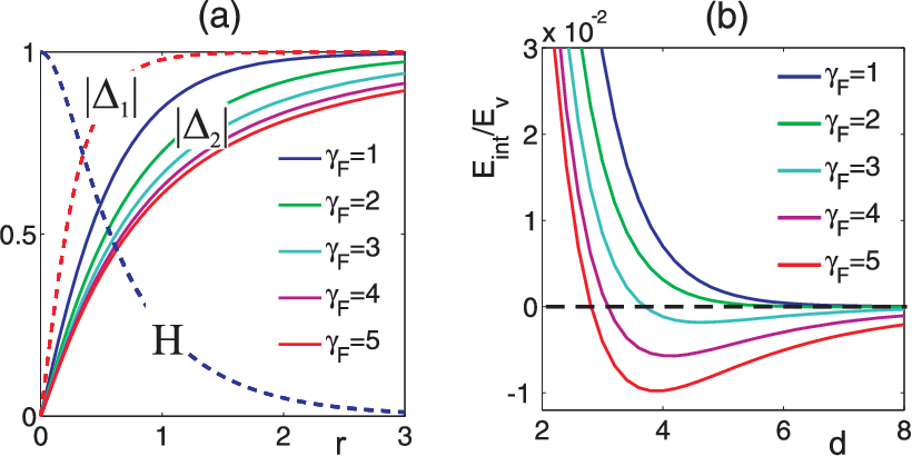
The temperature dependencies of the sizes of the vortex cores in two superconducting bands calculated in [12, 13] in the full nonlinear model according to the two alternative definitions. The first one is the slope of the gap function distribution at which characterizes the width of the vortex core near the center [Fig.(5)a]. The second one is the healing length defined as [Fig.(5)b] (i.e. this length is not directly related to exponents but quantifies at what length scales the gap functions almost recover their ground state values). Both definitions demonstrate the stretching of the vortex core in the weak component related to the peak of the coherence length shown in the Fig.(3)a. Note that the weak band healing length in Fig.(5)b has maximum at the temperature slightly larger than which is consistent with the fact that the maximum of coherence length (equivalently the minimum of the field mass ) in Fig.3a is shifted to the temperature above ( is defined as the lower critical temperature in the limit of no Josephson coupling).
Besides justifying the predictions of phenomenological two-component GL theory [13] the microscopic formalism developed in Ref.12 allows to describe type-1.5 superconductivity beyond the validity of GL models. The type-1.5 behavior requires a density mode with low mass to mediate intervortex attraction at large separations, which should coexist with short-range repulsion. The non-monotonic temperature behavior of the inverse coherence length shown in Fig.(3)a,b makes possible the attractive interaction between vortices. Furthermore because the softest mode with the mass in two band system may be associated with only a fraction of the total condensate (as follows from corresponding mixing angles), and because there could be the second mixed gap mode with larger mass , the short-range intervortex interaction can be repulsive marking the transition to the type 1.5 regime at low temperatures.

The microscopically demonstrated existence of two well defined coherence lengths [12, 13] and disparity of the characteristic length scales of variations of the densities two superconducting components shown in Fig.(4a) and (5) results in the type-1.5 superconductivity with physical consequences summarized in the table 1.
VII Conclusion
We reviewed the concept of type-1.5 superconductivity in multicomponent systems. Both at the levels of microscopic and Ginzburg-Landau theories the behavior arises as a consequence of the existence of several superconducting components with different coherence lengths in the system. In the type-1.5 regime one or several of coherence lengths are larger than the magnetic field penetration length , while other coherence lengths are smaller than . These coherence lengths are well defined not only for systems but also (under certain conditions) in case of multi-band systems with only symmetry. The concept also arises in systems with larger number of components and in particular in three band systems with broken time reversal, where the broken symmetry is [15]. The properties of this state are summarized in table 1. A more detailed review of this state is available in [17].
VIII Acknowledgments
EB was supported by Knut and Alice Wallenberg Foundation through the Royal Swedish Academy of Sciences, Swedish Research Council and by the US National Science Foundation CAREER Award No. DMR-0955902. MS was supported by the Swedish Research Council, ”Dynasty” foundation, Presidential RSS Council (Grant No. MK-4211.2011.2) and Russian Foundation for Basic Research. The computations were performed on resources provided by the Swedish National Infrastructure for Computing (SNIC) at National Supercomputer Center at Linkoping, Sweden.
References
- [1] V.L. Ginzburg and L.D. Landau, Zh. Eksp. Teor. Fiz. 20, 1064 (1950)
- [2] P.G. de Gennes, Superconductivity of metals and alloys (New York: Addison-Wesley, 1989).
- [3] L. Landau, Nature (London, United Kingdom) 141, 688 (1938). R. P. Huebener, Magnetic Flux Structures of Superconductors, 2nd ed. (Springer-Verlag, New-York, 2001). R. Prozorov, A. F. Fidler, J. Hoberg, P. C. Canfield, Nature Physics 4, 327 - 332 (2008); Ruslan Prozorov, Russell W. Giannetta, Anatolii A. Polyanskii, Garry K. Perkins, Phys. Rev. B 72, 212508 (2005)
- [4] A. Abrikosov Sov. Phys. JETP 5, 1174 (1957)
- [5] L. Kramer Phys. Rev. B 3, 38213825 (1971);
- [6] E. B. Bogomolny, Sov. J. Nucl. Phys. 24, 449 (1976) [Yad. Fiz. 24, 861 (1976)].
- [7] N.S. Manton and P.M. Sutcliffe, Topological Solitons (Cambridge University Press, Cambridge UK, 2004).
- [8] E. Babaev & J.M. Speight Phys.Rev. B 72 180502 (2005).
- [9] E. Babaev, J. Carlstrom, J. M. Speight Phys. Rev. Lett. 105, 067003 (2010).
- [10] Johan Carlstrom, Egor Babaev, Martin Speight Phys. Rev. B 83,174509, (2011).
- [11] V.V. Moshchalkov, M Menghini, T. Nishio, Q. H. Chen, A. V. Silhanek, V. H. Dao, L. F. Chibotaru, N. D. Zhigadlo, and J. Karpinski Phys. Rev. Lett. 102, 117001 (2009).
- [12] M. Silaev and E. Babaev, Phys. Rev. B 84, 094515 (2011).
- [13] M. Silaev and E. Babaev, Phys. Rev. B 85, 134514 (2012).
- [14] Johan Carlstrom, Julien Garaud, Egor Babaev Phys. Rev. B 84, 134515 (2011).
- [15] Johan Carlstrom, Julien Garaud, Egor Babaev arXiv:1107.4279; Phys. Rev. B 84, 134518 (2011)
- [16] Julien Garaud, Daniel F. Agterberg, Egor Babaev Phys. Rev. B 86, 060513(R) (2012)
- [17] E. Babaev, J. Carlstrom, J. Garaud, M. Silaev, J. M. Speight Physica C 479, 2-14 (2012); arXiv:1110.2744
- [18] T. Nishio, Q. Chen, W. Gillijns, K. De Keyser, K. Vervaeke, and V. V. Moshchalkov Phys. Rev. B 81, 020506(R) (2010); J. Gutierrez,, B. Raes , A. V. Silhanek, L. J. Li1, N. D. Zhigadlo, J. Karpinski, J. Tempere, and V. V. Moshchalkov Phys. Rev. B 85, 094511 (2012).
- [19] V. H. Dao, L. F. Chibotaru, T. Nishio, V. V. Moshchalkov Phys. Rev. B 83 020503 (2011).
- [20] G. Litak, T. Ord, K. Rago, A. Vargunin arXiv:1206.5486 , Physica C in print; T. Ord, K. Rago, A. Vargunin J.Supercond.Nov.Magn. 25 (2012) 1351-1356 Artjom Vargunin and Teet Ord Phys. Rev. B 86, 104506 (2012)
- [21] R. Geurts, M. V. Milosevic, F. M. Peeters Phys. Rev. B 81, 214514 (2010). A. A. Shanenko, M. V. Milosevic, F. M. Peeters, and A. V. Vagov. Phys. Rev. Lett. 106, 047005 (2011); L. Komendova, M. V. Milosevic, A. A. Shanenko, F. M. Peeters, Phys. Rev. B 84, 064522 (2011).A. Chaves, L. Komendova, M. V. Milosevic, J. S. Andrade Jr., G. A. Farias, F. M. Peeters Phys. Rev. B 83, 214523 (2011); L. Komendova, Yajiang Chen, A. A. Shanenko, M. V. Milosevic, F. M. Peeters Phys. Rev. Lett. 108, 207002 (2012); Juan C. Pina, Clecio C. de Souza Silva, Milorad V. Milosevic Phys. Rev. B 86, 024512 (2012)
- [22] Jun-Ping Wang, Physical Review B, 82, 132505 (2010); Shi-Zeng Lin, Xiao Hu Phys. Rev. B 84, 214505 (2011);
- [23] C.J. Olson Reichhardt, C. Reichhardt, A.R. Bishop Phys. Rev. E 83, 041501 (2011).
- [24] Xiao Hu, Zhi Wang Phys. Rev. B 85, 064516 (2012).
- [25] A. A. Shanenko, M. V. Milosevic, F. M. Peeters, and A. V. Vagov. Phys. Rev. Lett. 106, 047005 (2011); L. Komendova, M. V. Milosevic, A. A. Shanenko, F. M. Peeters, Phys. Rev. B 84, 064522 (2011). A. Vagov, A. A. Shanenko, M. V. Milosevic, V. M. Axt, and F. M. Peeters Phys. Rev. B 86, 144514 (2012) These works adopted the leading order of GL expansion from the work by Kogan and Schmalian [56] and calculated higher order corrections to it. The criticism of these results of Kogan and Schmalian [56] can be found in [58, 13]. Also, as shown recently in [13] the GL functionals similar to those used in the current MS are justified on formal grounds (in a certain range of parameters) contrary what was claimed in the above works.
- [26] G. Eilenberger and H. Buttner, Z. Physik 224, 335 (1969).
- [27] J. Halbritter, Z. Physik 243, 201 (1971).
- [28] K. Dichtel, Phys. Letters A 35, 285 (1971).
- [29] E. H. Brandt Phys. Letters A 39, 193 (1972).
- [30] A.E. Jacobs, Phys. Rev. B 4, 3016 (1971).
- [31] L. Neumann, L. Tewordt, Z. Phys. 189, 55 (1966).
- [32] M.C. Leung, A.E. Jacobs, Journal of Low Temp. Phys. 11 395, (1973).
- [33] M.C. Leung, Journal of Low Temp. Phys. 12, 215-235 (1973).
- [34] H. Suhl, B. T. Matthias, and L. R. Walker Phys. Rev. Lett. 3, 552 (1959).
- [35] A. Liu, I.I. Mazin, J. Kortus, Phys. Rev. Lett. 87 087005 (2001); I.I. Mazin, et al., Phys. Rev. Lett. 89 (2002) 107002.
- [36] X. X. Xi Rep. Prog. Phys. 71 116501 (2008).
- [37] A. Gurevich, Phys. Rev. B 67 184515 (2003).
- [38] I. N. Askerzade, A Gencer, N Guclu A Kilic Supercond. Sci. Technol. 15 L17L20 (2002)
- [39] A. Gurevich, Physica C 056 160 (2007).
- [40] M. E. Zhitomirsky and V.-H. Dao, Phys. Rev. B69, 054508 (2004).
- [41] A. E. Koshelev, A. A. Golubov Phys. Rev. Lett., 92, 107008 (2004).
- [42] K. Tanaka, M. Eschrig, D.F. Agterberg, Phys. Rev. B 75, 214512 (2007). K. Tanaka, D.F. Agterberg, J. Kopu, M. Eschrig Phys. Rev. B 73, 220501(R) (2006).
- [43] see e.g. K. Ishida, Y. Nakai,H., Hosono, J. Phys. Soc. Jpn. 78 062001 (2009).
- [44] L. J. Li , T. Nishio , Z. A. Xu , and V. V. Moshchalkov Phys. Rev. B 83, 224522 (2011).
- [45] N.W. Ashcroft, J. Phys. Condens. Matter 12, A129 (2000); Phys. Rev. Lett. 92, 187002 (2004).
- [46] E. Babaev, A. Sudbø and N.W. Ashcroft Nature 431 666 (2004).
- [47] E. Babaev, N.W. Ashcroft Nature Physics 3, 530 (2007).
- [48] E. Smørgrav, J. Smiseth, E. Babaev, A. SudbøPhys. Rev. Lett. 94, 096401 (2005).
- [49] E. V. Herland, E. Babaev, A. Sudbo Phys. Rev. B 82, 134511 (2010).
- [50] P. B. Jones, Mon. Not. Royal Astr. Soc. 371, 1327 (2006); E. Babaev, Phys. Rev. Lett. 103, 231101 (2009). B. Haskell, N. Andersson, G.L. Comer arXiv:1204.2894
- [51] S. A. Parameswaran, S. A. Kivelson, E. H. Rezayi, S. H. Simon, S. L. Sondhi, B. Z. Spivak Phys. Rev. B 85, 241307(R) (2012)
- [52] E.H. Brandt, M.P. Das J. Supercond. Nov. Magn. 24, 57 (2011).
- [53] G. Malescio and G. Pellicane, Nature materials, 2, 97 (2003). M. A. Glaser, G. M. Grason, R. D. Kamien, A. Kosmrlj, C. D. Santangelo and P. Ziherl EPL 78 4 (2007) 46004.
- [54] Pearl, J.: Appl. Phys. Lett. 5, 65 (1964)
- [55] R.P. Huebener Magnetic Flux Structures in Superconductors. Springer (2010).
- [56] V. G. Kogan, Joerg Schmalian Phys. Rev. B 83, 054515 (2011)
- [57] J. Geyer, R. M. Fernandes, V. G. Kogan, and J. Schmalian, Phys.Rev.B 82, 104521 (2010)
- [58] Egor Babaev, Mihail Silaev Phys. Rev. B 86, 016501 (2012) see also comment on reply of Kogan and Scmalian in Egor Babaev, Mihail Silaev arXiv:1105.3756