Epidemic thresholds of the Susceptible-Infected-Susceptible model on networks: A comparison of numerical and theoretical results
Abstract
Recent work has shown that different theoretical approaches to the dynamics of the Susceptible-Infected-Susceptible (SIS) model for epidemics lead to qualitatively different estimates for the position of the epidemic threshold in networks. Here we present large-scale numerical simulations of the SIS dynamics on various types of networks, allowing the precise determination of the effective threshold for systems of finite size . We compare quantitatively the numerical thresholds with theoretical predictions of the heterogeneous mean-field theory and of the quenched mean-field theory. We show that the latter is in general more accurate, scaling with with the correct exponent, but often failing to capture the correct prefactor.
pacs
89.75.Hc, 05.70.Ln, 87.23.Ge, 89.75.DaI Introduction
Models for disease propagation are a paradigmatic example of processes for which the interplay of a simple dynamics and a topologically complex interaction pattern [1, 2] gives rise to nontrivial phenomena [3, 4, 5, 6]. In this context, the Susceptible-Infected-Susceptible (SIS) model [7] plays a paramount role, as the simplest model undergoing an epidemic phase transition between an absorbing [8], healthy phase, where infection rapidly disappears, and an active phase, with a stationary endemic state characterized by a finite fraction of infected individuals. In the SIS model nodes can be either susceptible or infected. An infected node spreads the disease to each one of its susceptible contacts at rate , while it heals at a rate , usually taken to be 1. A critical value of the spreading rate separates the absorbing phase () from the endemic one ().
Traditional mathematical epidemiology has analyzed the behavior of the SIS model mainly within a mean-field (homogeneous mixing) approximation [7]. In this case, the epidemic transition occurs for a finite value of the control parameter, inversely proportional to the average connectivity of the interaction pattern. This view was completely revolutionized after the study of SIS on networks with large variations of nodes’ connectivities. The first mathematical approaches to SIS in networks [9, 10] were based on the heterogeneous mean-field (HMF) approach [4], an extension of standard mean-field theory taking explicitly into account the large fluctuations of the degree (number of connections) of single nodes, and that is based on replacing the actual topological structure of the network, given by its adjacency matrix 11 1 A matrix taking value if nodes and are connected and zero otherwise., by an average , expressing the probability that two vertices of degree and are connected in the original network (the so-called annealed network approximation [4]).
From here, an expression for the epidemic threshold is derived for uncorrelated networks22 2 Networks such that the probability that an edge arrives at a node of degree is proportional to [2]. [11]
| (1) |
where is the -th moment of the network’s degree distribution [1]. Eq. (1) predicts the epidemic threshold to vanish for networks with diverging second moment (“scale-free”), and to be finite otherwise. This result has huge implications, since many real networks have a power-law degree distribution with , so that grows unboundedly with the system size [1, 2, 5].
For almost a decade, HMF results for the SIS model were considered essentially correct in the case of random networks within the statistical physics community33 3 Its validity in random regular graphs has been however contested by means of a HMF pair approximation theory [12, 13], although no systematic detailed investigation of their accuracy was performed [14]. In other communities, however, different theoretical approaches have been applied, yielding opposite results. Chatterjee and Durrett [15, 16] have rigorously proven that, for strictly infinite system size, the epidemic threshold is exactly for any exponent of the degree distribution. Although of fundamental importance, this result does not provide a simple understanding of the physical origin of the threshold vanishing. Within the computer science community, another approximate approach, that we term quenched mean-field (QMF) theory, has been put forward by Wang et al. [17, 18]. The basic idea is to write down the evolution equation for the probability that a certain node is infected. Taking into account the actual connections in the network, as given by the adjacency matrix, this approach predicts the existence of a threshold given, for any graph, by the inverse of the largest eigenvalue of the adjacency matrix, namely
| (2) |
This result has been obtained later also by Gomez et al. [19] and, in a more refined way, by Van Mieghem et al. [20].
Equation (2) can be complemented with the expression for obtained by Chung et al. [21], to obtain an explicit estimate of the epidemic threshold [22]:
| (3) |
where is the largest degree in the network and and are numerical constants. This formula agrees with the result of Ref. [15] since the threshold vanishes for large as soon as diverges with , independently of [2]. The threshold (3) scales as the HMF result only for . The validity of the predictions of Eq. (3) has been qualitatively verified for scale-free and scale-rich networks in Ref. [22]. The physical origin of the different scaling for larger or smaller than has been clarified in Ref. [23]. However, a detailed investigation of the accuracy of the different theoretical approaches for generic graphs is still lacking.
It is important to stress that Eq. (2) is an improvement over HMF, but it is not exact. While in HMF theory the actual network structure is replaced by an annealed one [24], QMF theory fully preserves the detailed quenched structure of the network as described by the adjacency matrix. In fact, Eq. (1) can be derived from Eq. (2) by inserting the largest eigenvalue of the annealed network44 4 In annealed networks, the adjacency matrix takes a probabilistic interpretation, being replaced by the probability that two vertices and are connected. In degree uncorrelated networks, this annealed network adjacency matrix takes the form [4] (4) From this expression we can easily see that is an eigenvector of with eigenvalue . We can also see that . Since is a positive semidefinite matrix, all its eigenvalues are non negative, and since the trace is equal to the sum of the eigenvalues, it follows that the largest eigenvalue of the adjacency matrix in annealed networks is equal to , all the rest of the eigenvalues being equal to zero.. In this sense the HMF approach is equivalent to QMF theory plus an additional, annealed network, approximation. Yet both approaches rely on the mean-field (single-particle) assumption that the probability that nearest neighbor nodes are active can be factorized as the product of the single node probabilities. They thus neglect possibly important dynamical correlations between the state of adjacent nodes. For this reason, while it is appropriate to say that QMF approach improves over HMF, there is no guarantee about the exactness of Eq. (2), whose accuracy needs to be checked on a case-by-case basis.
In this paper we tackle this task, by performing large-scale numerical simulations of the SIS model on various types of graph, using the quasi-stationary method to study the phase-transition in finite systems [25], and determining the effective size-dependent threshold by analyzing the peak of the susceptibility [26]. The accuracy of the method is checked by applying it on heterogeneous annealed networks [27, 28, 24], in which HMF is exact [24, 29]. We then consider an example of homogeneous network, the random regular graph, and an instance of strongly heterogeneous network, the star network. In the first case, we observe that both HMF and QMF predict finite thresholds, close to the numerical one, but not equal to it. In the second case, QMF correctly predicts the scaling of the vanishing threshold with network size, but the prefactor is not the right one. Finally, we consider the key case of power-law degree distributed networks. For both theories turn out to give an asymptotically exact value for the threshold. For we observe a vanishing threshold whose scaling with is correctly predicted by QMF, although with an incorrect prefactor. For we numerically recover the presence of two competing activation mechanisms discussed in Ref. [23]: QMF prediction follows approximately the transition due to the activation of the largest hub in the network, which vanishes and dominates in the large size limit. The HMF threshold remains finite and is close to the transition point due to the most densely connected core of the network (maximum -core).
Our numerical results confirm that QMF is indeed an improvement over HMF, providing a better estimate of the threshold and capturing the vanishing threshold for power-law distributed networks with any , a key fact missed by the HMF approach. However, it is only the scaling of the threshold with network size that is correctly given by QMF. Improved analytical strategies, beyond quenched mean-field are thus needed in order to obtain more accurate threshold predictions in cases of practical importance. After submission of this paper, we became aware of a publication [30] in which a similar numerical comparison is performed on much smaller network sizes than those considered here.
II Numerical methods
We consider here the SIS model for epidemics in continuous time. The numerical algorithm is implemented as follows: At each time step, we compute the number of infected nodes, , and links emanating from them, . With probability one infected node, chosen at random, becomes healthy. With complementary probability , one of the links is selected uniformly at random and the infection is transmitted through it from the infected node corresponding to one of the ends of the edge, towards the (possibly susceptible) node at the other end. The numbers of infected nodes and related links are updated accordingly, time is incremented by , and the whole process is iterated.
II.1 The quasi-stationary state method
The standard numerical procedure to investigate the properties of absorbing phase transitions is based on the determination of the average of the order parameter (in this case the density of infected nodes), restricted only to surviving runs [8], i.e., runs which have not reached the absorbing state up to a given time . Such a technique is quite wasteful, because surviving configurations are very rare at long times close to the threshold, and an exceedingly large number of realizations of the process are needed in order to get substantial statistics. An alternative technique is the quasi-stationary state (QS) method [25, 29], based on the idea of constraining the system in an active state. This procedure is implemented by replacing the absorbing state, every time the system tries to visit it, with an active configuration randomly taken from the history of the simulation. For this task, a list of active configurations, corresponding to states previously visited by the dynamics, is stored and constantly updated. An update consists in randomly choosing a configuration in the list and replacing it by the present active configuration with a probability . After a relaxation time , the QS quantities are determined during an averaging time . The QS probability that vertices are infected is computed during the averaging interval, each configuration with active vertices contributing to the QS distribution with a probability proportional to its lifespan . From the particle distribution , the moments of the activity distribution can be computed as
| (5) |
The simulation procedure described above was recently used to determine with high numerical accuracy the critical point and exponents of the contact process [8] on annealed [29] and quenched [31] networks with power law degree distributions.
The values of the QS parameters used in the present simulations were and , while and varied depending on and .
II.2 Numerical determination of the epidemic threshold
In usual absorbing-state phase transitions, where the critical point converges to a finite value in the thermodynamic limit, the finite-size scaling method allows the precise numerical determination of the critical point and the whole set of associated critical exponents [8]. It is based on the computation, for increasing system sizes , of , the global activity density, computed from surviving run averages or from QS simulations. For values of the control parameter in the active phase, reaches a finite non-zero limit as . For values of the control parameter in the absorbing phase, decays trivially as , since there is essentially of the order of one active vertex in the whole network. The critical point is distinguished by a power-law decay , where is the critical exponent controlling the density at a finite distance from the critical point, while is associated to the growth of correlations close to criticality [8].
In networks with a diverging second moment for the degree distribution, this approach can go awry if strong corrections to scaling are present [29, 31]. In the particular case of the SIS model on networks with a power-law degree distribution, this approach simply does not work, because the effective threshold depends on and it goes to zero as the system size grows. Therefore, for any value of , will attain a finite limit for a sufficiently large , once the corresponding becomes smaller than . This shows that asymptotically the threshold is zero [22], but it does not provide information on the effective threshold for finite . To overcome this problem, we turn instead to another procedure to determine the critical point, namely the study of the susceptibility [26], defined as
| (6) |
When plotted as a function of in a system of fixed size , the susceptibility exhibits a maximum at a value . In systems with a finite critical point in the thermodynamic limit , the peak of the susceptibility at corresponds to a transition rounded by finite size effects, that as tends to the critical point as [26]. Correspondingly, the height of the susceptibility at the maximum scales with system size as , where is a new critical exponent.
We assume that the relation between and written above holds also in the present case, where depends on : . This implies that the susceptibility peak and the size-dependent threshold tend to coincide in the large size limit. When the assumption can be explicitly controlled, it turns out (see below) to be correct.
III Numerical check of the susceptibility method: Annealed scale-free networks
A natural benchmark to check the accuracy of the susceptibility peak as a measure of the position of the critical point in the SIS model is given by annealed networks [27, 28, 24]. In annealed networks, all edges are rewired (preserving the degree and the degree correlations of the involved nodes) after each change of the state of any vertex. This procedure destroys all dynamical correlations, and thus renders exact the prediction of HMF theory [4, 24]. From a practical point of view, the regeneration of the whole network every time a microscopic dynamic step is performed can be effectively achieved in uncorrelated networks by selecting at random, every time that a nearest neighbor of a vertex is needed, a vertex of degree , with probability [24].


In Fig. 1 we present the results of susceptibility measurements for uncorrelated annealed networks with degree exponent , and . Fig. 1(a) depicts the susceptibility defined in Eq. (6) and the usual susceptibility defined in the analysis of absorbing phase transition [8], in networks with and different sizes . We observe that provides a more clear-cut definition of the susceptibility peak. The same behavior is observed for (data not shown). In Fig. 1(b) we plot the evolution of the susceptibility peak as a function of network size for fixed and , and compare it with the numerically evaluated HMF prediction. These results confirm that provides an excellent approximation of the exact result , both when the threshold goes to zero with and when it converges to a finite value. The differences observed might be attributed to corrections to scaling, such as those presented in systems with a finite threshold in the thermodynamic limit, see Sec. II.2. Therefore, in the rest of the paper we use the position of the peak of the susceptibility as the numerical estimate of the position of the threshold.
IV Homogeneous networks: The random regular network
As a first non-trivial application of the technique of the susceptibility peak to evaluate the SIS epidemic threshold in homogeneous networks, we consider the case of random regular networks (RRN) that is, networks where all nodes have exactly the same degree , while links are randomly distributed among them, avoiding self-connections and multiple connections. In this case, HMF theory predicts trivially a constant threshold . The prediction of QMF theory takes exactly the same value, as can be easily seen by applying Perron-Frobenius theorem 55 5 It is easy to see that is an eigenvector of the adjacency matrix with eigenvalue . Therefore, the result derives directly from Perron-Frobenius theorem [32]..

Fig. 2 shows the susceptibility as a function of for RRNs with increasing and degree . The numerical estimated threshold is quite off from the theoretical value for HMF and QMF, indicating that both theories are essentially incorrect, while the susceptibility peak falls close (increasingly so for larger ) to the value , which is the prediction of the pair approximation [33].
From this analysis we conclude that HMF and QMF provide a reasonable approximation but not the exact position of the threshold. They fail just because they neglect dynamical correlations among the state of neighbors, which are instead better taken into account by pair approximation approaches [12, 13].
V Heterogeneous networks: The star graph
In this Section we focus on the simplest case of a heterogeneous network with vanishing epidemic threshold, namely the star network, which is composed by a hub of degree , to which leaves of degree are attached. For this star graph, the largest eigenvalue of the adjacency matrix can be easily shown66 6 The adjacency matrix of the star graph can be represented by for and , otherwise. Therefore, if is an eigenvector of , we have: (i) and (ii) for . Replacing in equation (i) and using we found the result . to be . Therefore the QMF prediction from Eq. (2) is . On the other hand, the HMF result from Eq. (1) takes in this case the form .
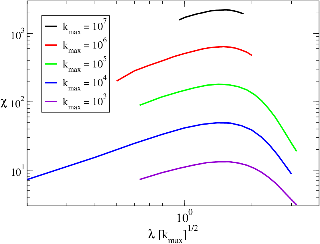
Figure 3 shows the susceptibility versus computed for star graphs with a wide range of values of . It clearly shows that the scaling is correct, however the value of the prefactor is around , rather than 1, in agreement with the rigorous bound derived by Ganesh et al. [34]. The star graph constitutes thus the simplest example of a network for which HMF theory does not work. This failure of HMF is altogether not surprising, since this particular network is strongly correlated at the degree level, and therefore fails to fulfill one necessary condition for the validity of the HMF result Eq. (1). QMF theory instead provides the correct scaling of the threshold with network size, although the prefactor is not exact.
VI Heterogeneous Networks: Power-law degree distributed graphs
We now consider the SIS model on networks with power-law degree distributions, , built using the uncorrelated configuration model (UCM) [35]. This procedure is equal to the standard Molloy-Reed configuration model [36] with the additional constraint that the degree values are strictly bounded by . This bound guarantees that no topological correlations are present in the network [37], and therefore fulfills the requirement needed for the applicability of the HMF result Eq. (1).
We analyze three values of , representative of three regimes characterized by different expressions for the theoretical estimates.
VI.1

In Fig. 4 we show the shape of the susceptibility versus (inset) and the numerical threshold as a function of the network size (main plot) for , compared with the predictions of the two theoretical approaches. It turns out that the numerical results from the susceptibility peak agree with good accuracy with both HMF and QMF theories, which in their turn tend to coincide. While it was expected that the theoretical formulas scaled in the same way with , see Eq. (3), the fact that they tend to coincide indicates that the prefactor in Eq. (3) is . Fig. 4 shows that HMF and QMF predictions are apparently exact in the limit of large systems for .
In this particular range of , since the transition can be identified with high accuracy, it is possible to extract additional information about the epidemic phase transition. We consider thus the scaling of the quantities , and with at the transition point. According to standard notation [8], the expected scaling with system size should be (see Sec. II.2):
| (7) |


In Fig. 5(a) we plot the values of , and , evaluated at the susceptibility peak, as a function of in SF networks with . Fitting the curves in Fig. 5(a) to a power law form, we find the exponents:
| (8) |
These exponents explain why is the best choice to determine the threshold. The maximum of the standard susceptibility scales with a negative exponent , and thus, in the limit of large , the transition is characterized by a discontinuity. The value instead ensures a clearly defined maximum for the susceptibility diverging as .
By plotting the order parameter as a function of the distance from the effective threshold, we can attempt to determine the exponent , which is defined by . In Fig. 5(b) we show such a plot, for a SF network with and size . According to HMF theory [9], the exponent is expected to take the value , while the QMF approach of Van Mieghem [38] predicts . The numerical results presented in Fig. 5(b) yield an effective exponent lying between the theoretical predictions, so that the validity of none of them can be excluded.
VI.2
In this interval of , Eq. (3) predicts that a different regime sets in, with the threshold set by the inverse of the square-root of i.e. , while HMF theory predicts up to . For the values of which can be simulated numerically, the two theoretical predictions are quite close but do not coincide.

Figure 6 shows the results of the susceptibility analysis for SF networks with . From this plot, we conclude that the numerical results do not conform to the HMF behavior, the more so for large system size. The numerical threshold scales instead as the inverse of the largest eigenvalue, but with a prefactor different from unity. The QMF threshold provides hence an approximation to the numerical threshold, scaling in the same way, but with an accuracy of the order of .
VI.3
For , HMF theory yields a finite value of the threshold, which instead still vanishes according to QMF. Since sample-to-sample fluctuations of the value of are quite large in this regime, we consider for each value of only networks with equal to the mean value [22].


In Fig. 7(a) we plot the susceptibility as a function of in networks with . The behavior of the susceptibility in this regime is remarkably different from the one observed in the case . As we can see, while for small network sizes a well defined and unique peak is present for relatively large values of , at a position quite compatible with the prediction of HMF, as grows another feature emerges for smaller values of , giving rise to a secondary peak for the largest considered sizes.

The evidence presented in Fig. 7(a) can be better understood with the help of the QS distribution of the order parameter (number of active nodes ) depicted in Fig. 8. For large values of , the distribution has a single peak (apart from the one in .). As is reduced, a secondary peak starts to appear at smaller values of and rapidly takes over. Further decreasing leads to the disappearance of the all peaks for finite , which signals the transition into the absorbing state.
Figs. 7(a) and 8 reflect the existence of two competing thresholds, associated to two different mechanisms triggering the transition [23]. The secondary peak for small , whose position scales with network size as predicted by QMF formula, see Fig. 7(b), is associated to the presence of the star-subgraph centered around the largest hub, which for is able to sustain alone the active state [22, 23]. This kind of transition starts from a localized region [39] and then propagates the infection to the rest of the network. Its position is set by and does not change depending on the quenched network realization. Notice also the rounded shape of the susceptibility peak, reminiscent of the what is found for star graphs (see Fig. 3). The peak for large , which occurs not far the value predicted by HMF and is much narrower, is associated to the set of most densely connected nodes in the network (maximum -core) collectively turning into the active state. The location of this transition fluctuates a lot depending on the realization.
It is clear that for asymptotically large the first mechanism dominates. In this limit one expects the picture to be analogous to the case presented above: a single peak moving toward zero as increases, as predicted by Eq. (2) (but with a different prefactor). However, the crossover to this stage is very slow and values of much larger than those attainable with our computational resources would be needed to check in detail the accuracy of Eq. (2) in this regime.
VII Conclusions
In this paper we have presented a large scale numerical analysis of the SIS model on networks. Our approach presents two improvements over previous numerical studies of the SIS. Firstly, we have implemented the quasi-stationary state (QS) method, which allows to overcome the problems associated to simulations based on surviving averages, yielding far better statistics with much smaller uncertainties. Secondly, to overcome the problems that traditional finite-size scaling analysis face in front of a vanishing critical point, we have instead considered the susceptibility , whose maximum value provides a numerical estimate of the threshold. The combination of the QS and susceptibility peak methods leads to numerically accurate threshold estimates, as we have checked in the case of annealed networks, in which the exact value of the SIS threshold is known. The accuracy of our results allows us to discuss in detail the relative performance of two candidate theoretical solutions to the SIS model on networks, namely the heterogeneous mean-field (HMF) and the quenched mean-field (QMF) theories.
By considering the very simple case of the random regular graph, our analysis shows that even for homogeneous networks, which have a finite threshold for large sizes, both HMF and QMF theories may provide inaccurate results. This occurs because dynamical correlations play a role in determining the threshold value, but they are disregarded by the theoretical approaches.
In the case of strongly heterogeneous networks (the star graph), QMF theory is sufficient to yield the correct scaling, but errs in the associated prefactor, again due to dynamical correlations.
Turning to the more interesting case of random uncorrelated scale-free networks, our numerical results indicate that both HMF and QMF provide asymptotically exact expressions for the epidemic threshold in the case . In the region , both theories are quite close for the investigated sizes but QMF is able to reproduce the scaling of the threshold with network size, erring only in the numerical prefactor. The analysis of the more complex case leads to a picture in agreement with the presence of two epidemic activating mechanisms discussed in Ref. [23]. Here, the susceptibility presents for small network sizes a peak at large , close to the HMF prediction, which tends to a finite limit but largely fluctuates from sample to sample. This peak is associated to the activation of the epidemics in the network by the set of most densely connected nodes in the network (maximum -core). For large sizes, a secondary incipient peak appears at small , which is described by QMF and asymptotically overcomes the other peak at sufficiently large . The secondary peak is associated to the epidemic activation from the most connected node in the network which, as center of a star graph of size , is able, all alone, to sustain activity in the whole network.
From our numerical assessment of the validity of HMF and QMF theories we can conclude that, while QMF represents a notable improvement over the HMF approach, it is still unable to yield a precise determination of thresholds, apart from the special case . This calls thus for improved analytical approximations, which should include in an explicit manner the effects of dynamical correlations between neighboring nodes. Progress has been done recently along this path [12, 13, 33], but these methods are easily applicable only to small networks, so that the precise theoretical determination of the SIS epidemic threshold for large networks remains essentially an open problem.
Acknowledgements.
SCF thanks financial support of the Brazilian agencies CNPq and FAPEMIG. CC acknowledges financial support from the European Science Foundation under project DRUST. R.P.-S. acknowledges financial support from the Spanish MEC, under project No. FIS2010-21781-C02-01; the Junta de Andalucía, under project No. P09-FQM4682; and additional support through ICREA Academia, funded by the Generalitat de Catalunya.References
- [1] R. Albert and A.-L. Barabási, Rev. Mod. Phys. 74, 47 (2002)
- [2] S. N. Dorogovtsev and J. F. F. Mendes, Adv. Phys. 51, 1079 (2002)
- [3] A. Barrat, M. Barthélemy, and A. Vespignani, Dynamical Processes on Complex Networks (Cambridge University Press, Cambridge, 2008)
- [4] S. N. Dorogovtsev, A. V. Goltsev, and J. F. F. Mendes, Rev. Mod. Phys. 80, 1275 (2008)
- [5] M. Newman, Networks: An Introduction (Oxford University Press, Inc., New York, NY, USA, 2010)
- [6] A. Vespignani, Nature Physics 8, 32 (2012)
- [7] R. M. Anderson and R. M. May, Infectious diseases in humans (Oxford University Press, Oxford, 1992)
- [8] J. Marro and R. Dickman, Nonequilibrium phase transitions in lattice models (Cambridge University Press, Cambridge, 1999)
- [9] R. Pastor-Satorras and A. Vespignani, Phys. Rev. E 63, 066117 (2001)
- [10] R. Pastor-Satorras and A. Vespignani, Phys. Rev. Lett. 86, 3200 (2001)
- [11] M. Boguná and R. Pastor-Satorras, Phys. Rev. E 66, 047104 (2002)
- [12] Proc. Natl. Acad. Sci. USA 99, 13330 (2002)
- [13] J. P. Gleeson, Phys. Rev. Lett. 107, 068701 (2011)
- [14] D. Hwang, S. Boccaletti, Y. Moreno, and R. Lopez-Ruiz, Mathematical Biosciences and Engineering 2, 317 (2005)
- [15] S. Chatterjee and R. Durrett, Ann. Probab. 37, 2332 (2009)
- [16] R. Durrett, Proc. Natl. Acad. Sci. USA 107, 4491 (2010)
- [17] Y. Wang, D. Chakrabarti, C. Wang, and C. Faloutsos, in 22nd International Symposium on Reliable Distributed Systems (SRDS’03) (IEEE Computer Society, Los Alamitos, CA, USA, 2003) pp. 25–34
- [18] D. Chakrabarti, Y. Wang, C. Wang, J. Leskovec, and C. Faloutsos, ACM Trans. Inf. Syst. Secur. 10, 1 (2008)
- [19] S. Gómez, A. Arenas, J. Borge-Holthoefer, S. Meloni, and Y. Moreno, Europhys. Lett. 89, 38009 (2010)
- [20] P. Van Mieghem, J. Omic, and R. Kooij, IEEE ACM T. Network. 17, 1 (2009), ISSN 1063-6692
- [21] F. Chung, L. Lu, and V. Vu, Proc. Natl. Acad. Sci. USA 100, 6313 (2003)
- [22] C. Castellano and R. Pastor-Satorras, Phys. Rev. Lett. 105, 218701 (2010)
- [23] C. Castellano and R. Pastor-Satorras, Sci. Rep. 2, 371 (2012)
- [24] M. Boguñá, C. Castellano, and R. Pastor-Satorras, Phys. Rev. E 79, 036110 (2009)
- [25] M. M. de Oliveira and R. Dickman, Phys. Rev. E 71, 016129 (2005)
- [26] K. Binder and D. W. Heermann, Monte Carlo Simulation in Statistical Physics, 5th ed. (Springer-Verlag, Berlin, 2010)
- [27] S. Gil and D. Zanette, Eur. Phys. J. B 47, 265 (2005)
- [28] D. Stauffer and M. Sahimi, Phys. Rev. E 72, 46128 (2005)
- [29] S. C. Ferreira, R. S. Ferreira, and R. Pastor-Satorras, Phys. Rev. E 83, 066113 (2011)
- [30] C. Li, R. van de Bovenkamp, and P. Van Mieghem, Phys. Rev. E 86, 026116 (2012)
- [31] S. C. Ferreira, R. S. Ferreira, C. Castellano, and R. Pastor-Satorras, Phys. Rev. E 84, 066102 (2011)
- [32] F. R. Gantmacher, The Theory of Matrices, Vol. II (Chelsea Publishing Company, New York, 1959)
- [33] E. Cator and P. Van Mieghem, Phys. Rev. E 85, 056111 (2012)
- [34] A. Ganesh, L. Massoulié, and D. Towsley, in IEEE INFOCOM (2005) pp. 1455–1466
- [35] M. Catanzaro, M. Boguñá, and R. Pastor-Satorras, Phys. Rev. E 71, 027103 (2005)
- [36] M. Molloy and B. Reed, Random Struct. Algor. 6, 161 (1995)
- [37] M. Boguñá, R. Pastor-Satorras, and A. Vespignani, Eur. Phys. J. B 38, 205 (2004)
- [38] P. V. Mieghem, Europhys. Lett. 97, 48004 (2012)
- [39] A. V. Goltsev, S. N. Dorogovtsev, J. G. Oliveira, and J. F. F. Mendes, Phys. Rev. Lett. 109, 128702 (2012)