Thermodynamic instabilities in dynamical quark models with complex conjugate mass poles
Abstract
We show that the CJT thermodynamic potential of dynamical quark models with a quark propagator represented by complex conjugate mass poles inevitably exhibits thermodynamic instabilities. We find that the minimal coupling of the quark sector to a Polyakov loop potential can strongly suppress but not completely remove such instabilities. This general effect is explicitly demonstrated in the framework of a covariant, chirally symmetric, effective quark model.
pacs
12.38.Aw, 12.39.-x, 11.30.Rd, 25.75.NqI Introduction
The fate of hadronic matter in extreme environments, e.g., in the interior of compact stars or in the early universe, remains one of the most interesting unanswered questions today. Heavy-ion experiments performed at the Relativistic Heavy-Ion Collider (RHIC) at the Brookhaven National Laboratory or at the Large Hadron Collider (LHC) at CERN Geneva show that at sufficiently high temperature or density, hadronic matter undergoes a phase transition by dissolving into its constituents: quarks and gluons. Details of this transition are encoded in the phase diagram of quantum chromodynamics (QCD).
Due to its non-perturbative nature at low temperatures and densities, QCD is best studied on the lattice in this regime. Results for the QCD equation of state (EoS) have recently become available also at physical quark masses and were extrapolated to the continuum [1, 4, 2, 3, 5, 6, 7, 8]. However, at finite densities lattice simulations are still limited due to the known sign problem.
In this situation, effective models of QCD serve to interpret and also extrapolate lattice results. To be realistic, such a model must dynamically break chiral symmetry and confine the colored degrees of freedom. In particular, quark and gluon propagators should strongly differ from their high-energy counterparts. A suitable continuum, non-perturbative and covariant approach is provided by the Dyson-Schwinger equations (DSE) (for reviews see e. g. [9, 10, 11]) and its descendants, the non-local chiral quark models [12, 13, 14, 15] (see also [16, 17, 18]), most recently augmented by the Polyakov loop (PL) [19, 20, 21, 22, 23, 24, 25, 26].
A non-perturbative quark propagator is a solution of its DSE, within the appropriate symmetry-preserving truncation scheme. The most crucial behavior of these continuum studies is a strong infrared running of the quark dynamical mass, which is to be interpreted as dynamical chiral symmetry breaking (DChSB), and of the wave function renormalization. Confinement can be realized through the absence of poles of the quark propagator at real time-like four-momenta by the criteria of positivity violation [9, 10]. Indeed, it is a common feature that, due to strong dynamics, the poles are pushed deep into the complex four-momentum region [27, 28, 29, 30, 31, 32]. The most simple resulting structure is a series of quartets of complex conjugate mass poles (CCMPs).
For a successful phenomenological study it is sufficient to model the strong interactions via an effective gluon propagator to be fixed by the infrared observables in the vacuum. Enhancement of the interaction in the infrared pushes the quark poles away from the real axis. Another possible realization is the absence of propagator poles in the entire complex plane which can be realized either by the presence of cuts instead of poles [33] or by the absence of both when the quark propagator is obtained as an entire function [34, 35]. A non-constant entire function must have a singularity at infinity. In order for such a quark state to become deconfined and to restore its approximate chiral symmetry, e.g., at high temperature, the gluon sector of the theory must be restructured in the transition region in order to allow for the appropriate changes in the analytic properties of the propagators such as the appearance of quasiparticle poles. But in that case, the usual strategy is no longer applicable: to predict the behavior at finite temperature and chemical potential from a straightforward generalization using the Matsubara formalism without changing the analytic properties which were adjusted by constraints from vacuum observables. A modification of this strategy lies beyond the scope of the present study.
A CCMP structure in the quark propagator is sufficient to ensure violation of reflection positivity [30, 32, 36], and as such provides a useful form to fit the lattice quark propagator [32, 36]. This led to applications at finite quark chemical potential [37], or for parton distribution functions [38]. On the other hand, QCD bound states are affected by this structure [39], e.g., a sufficiently heavy meson state (typically of the order of GeV) has unphysical thresholds [40] if a näive analytic continuation to the mass pole of the bound state is used (see [12] for a suggestion how this problem could be circumvented by a more elaborate analytic continuation).
In this work we want to further investigate the properties of models with CCMPs by concentrating on the finite temperature and finite quark chemical potential EoS. We find that the pressure of quark matter leads to an unsatisfactory scenario; the EoS exhibits oscillations in temperature which are in turn a consequence of the imaginary part of the CCMPs. We provide analytic insight into the nature of these oscillations, and suggest a partial solution to this problem by coupling the system to the Polyakov loop (PL).
This paper is organized as follows. In Section II, we present our arguments in a general form by postulating a CCMP parametrization of the quark propagator for which we then obtain the kinetic part of the QCD partition function in the quark sector. This result elucidates that the presence of complex conjugated mass poles in the quark propagator entails thermodynamic instabilities. We introduce the PL variable in the partition function and show that this step very effectively suppresses the instability. A separate analysis is performed for the EoS at zero temperature where for the CCMP parametrization the quark number density and the pressure can be obtained in closed form. In Section III we present the example of dynamical quark models with chirally invariant nonlocal interaction, including explicit numerical results and their discussion. In Section IV we give the summary and conclusions of our study.
II Thermodynamics in the CCMP representation
The (unrenormalized) thermodynamic potential for the quark sector of QCD can be given in the form of the Cornwall-Jackiw-Tomboulis (CJT) effective action [41] as
| (1) |
where represents the inverse of the full quark propagator in Euclidean space,
| (2) |
The quark dressing functions and encode effects of the quark selfenergy , expressing all deviations from the free propagator due to nonperturbative interaction effects. At finite temperature and chemical potential the “shifted” fermionic Matsubara frequencies with temperature and chemical potential , are introduced, so that . For the free quark propagator we have and , the current quark mass. The operation implies summation over internal degrees of freedom and . The leading term in the 2PI loop expansion is the usual one-loop contribution which we denote as the kinetic contribution to the thermodynamic potential of the system
| (3) |
and the functional contains all higher loop diagrams. In the widely used rainbow-ladder approximation (see e.g. [9]) it is given by
| (4) |
A quite general and mathematically simple realization of the analytic structure of the quark propagator exhibits a series of CCMPs in the plane for and, . The complex numbers are ordered such that . Let us for definiteness assume that all the poles are simple. The following arguments can easily be generalized if the quark propagator has higher order poles, or branch cuts. At zero three-momentum the pole structure in the plane is a series of quartets of poles located at and , and we define such that for all . With the poles are given by [13]
| (5) |
where for each their locations form a quartet in the complex energy plane at and , with
| (6) |
The analytic structure of the quark propagator governs the thermodynamical properties of the system. Here we perform a simple calculation of the kinetic contribution to the thermodynamic potential in the quark sector, with the proposed form of the quark propagator.
II.1 Consequences for the quark sector at finite temperature
Performing the trace in Dirac, color, flavor and momentum space, the kinetic term can be written as
| (7) |
For simplicity we work with equal flavors. is the number of colors.
In order to perform the Matsubara sum we introduce generalized occupation numbers
| (8) |
having simple poles at . With the help of the residue theorem, the Matsubara sum is converted to an integral along straight lines and , where is infinitesimal
| (9) |
where we defined
| (10) |
Here and in the following we suppress the dependence in for brevity.
Due to the known analytic structure of the quark propagator the integrals in (9) can be evaluated. We now close the contour running from to by a large semicircle on the positive real axis, and denote this as . Then we can rewrite
| (11) |
where the first equality follows from partial integration. The last line is the result of the residue theorem, and are the previously defined poles.
For the second term we first make use of the clockwise oriented contour defined as a rectangle having vertices in to obtain
| (12) |
If the second term in (12) is rewritten using , the first of the two resulting terms can be Wick rotated to the real axis, providing the vacuum contribution, while the second term can be evaluated by yet another contour, defined as , where we close the line running from to by a large semicircle on the negative real axis. This gives
| (13) |
Collecting the obtained formulas, we can state the kinetic contribution to the pressure
| (14) |
where is the (divergent) zero-point energy contribution
| (15) |
It is plain to see that in the special case of just one pair of real poles at , the original dispersion (6) is reduced to the one of a free relativistic particle, and, accordingly, the second term in Eq. (14) is reduced to the free Fermi gas expression, a situation also encountered, e.g., in the Nambu Jona-Lasinio (NJL) model [42, 43], see, e.g., [44, 45, 46, 47]. In the first term, the integral over can be evaluated as well, leading to
which, again in the case of a pair of real poles, is just the usual zero-point energy.
By combining the logarithms, (14) can be cast in a more transparent form
| (16) |
Note that the oscillating cosine functions in the thermodynamic potential could render the quark matter unstable. Their origin is traced back to the appearance of imaginary parts of the quark mass poles.
II.2 Introducing the Polyakov loop
The traced PL and its conjugate are order parameters for confinement in quenched QCD [48, 49], and as such represent important configurations of the gluon field that should be accounted for in the effective thermodynamic description of QCD. They are given as thermal expectation values
| (17) |
where is the untraced PL. In the Polyakov gauge [48] the latter takes a simple form , where are color Gell-Mann matrices, with being the background gluon field. Quark (antiquark) confinement is then signalled by ().
Coupling of the PL to the quarks amounts to a modification of the quark occupation number function
| (18) |
Following the same steps as in the previous subsection, the kinetic contribution to the thermodynamic potential can be written as
| (19) |
Working out the color trace gives
| (20) |
Again, in the special case of just one pair of real poles at , this expression is reduced to the corresponding term of the Polyakov-Nambu-Jona-Lasinio (PNJL) model (see, e.g., [50, 51, 52, 53]).
The logarithms can be combined to obtain
| (21) |
Comparing this with Eq. (16), we see that now the dominant cosine terms are weighted by the PL. As a consequence, the pressure instabilities are highly suppressed in the confined phase: As long as and are zero, there remains only one cosine term, which is, however, suppressed by the third power of the Boltzmann factor. In fact, the mechanism is basically the same as in the PNJL model, where the coupling to the PL suppresses the quark degrees of freedom at low , but does not eliminate them entirely [51, 52, 53].
II.3 Zero temperature, finite chemical potential
In this part, special attention is devoted to the effects of the CCMPs along the , axis. The Matsubara sum in (7) gets converted to an integral over .
| (22) |
where
We start by considering the quark number density
| (23) |
where is given by (10). At zero chemical potential, the quark density is zero, as it is obvious from the integrand being an odd function of . This allows for the evaluation of the integral by a clockwise oriented rectangular contour in the complex plane having vertices in . As the poles (6) are defined in Minkowski space, in Euclidean space this means that the only poles that enter the contour have . Therefore
| (24) |
The residue can straightforwardly be shown to be in both cases, giving
| (25) |
The theta function defines a “generalized” Fermi momentum
| (26) |
The quark number density can now be obtained as
| (27) |
It is actually remarkable that the density thresholds depend only on the real parts, . The imaginary parts enhance the Fermi momenta (and thus the density) compared to the values one would get for . For and
the Fermi momentum is even larger than . This point will later become important.
Integrating the expression
the thermodynamic potential can be reconstructed in a closed form
where
| (28) |
It is straightforward to see that in the case of only a pair of real mass poles we get the familiar expression for the free, massive, relativistic Fermi gas
| (29) |
We mention that at zero temperature the PL decouples, so it has no effect on the EoS.
III Instabilities in a non-local chiral quark model
The dispersion relations which enter Eq. (14) are governed by the analytic structure of the quark propagator, so that further insight can be obtained only by studying the thermal behavior of the quark propagator, i.e., by understanding how the CCMPs respond to a change in the temperature or density.
Parametrizing the analytic structure, say, from lattice studies at finite is very demanding. In this case the analytic structure is also somewhat arbitrary as the quark propagator is known only at a finite number of points, allowing for different meromorphic forms [32]. For the present purpose we will therefore study a specific model as an example case. More precisely, we consider a Dyson-Schwinger model with a separable gluon interaction [12, 16, 17]. In the rainbow-ladder approximation, these models are in fact identical to mean-field non-local NJL models, see, e.g., [21, 24, 25]. They capture the important aspect of momentum dependent dressing functions in the quark propagator (2) by introducing regulator functions which also ensure the convergence of loop integrals. Here we consider the particularly simple rank-1 case, where , while
| (30) |
with being the chiral symmetry breaking parameter (mass gap) and the regulator function. The latter is an input of the model.
For this kind of separable models, it was already observed in the literature that pressure instabilities appear in certain regions of the - plane. In Refs. [16, 13, 14, 15, 54] this was found in full numerical studies, and in [54] also by restricting the calculations to a finite number of CCMPs. The aim of the present section is to demonstrate that these instabilities are driven by the presence of the CCMPs, and then to study the effect of the PL. Results from a full numerical study will be confronted with a calculation where we restrict ourselves only to a finite number of CCMPs, demonstrating that the instability region is actually completely dominated by the first quartet.
III.1 Analytic structure
The analytic structure of the model was detailed in Refs. [13, 14, 15] for Gaussian and Lorentzian regulators. We briefly summarize their analysis for the case of the Gaussian regulator, given by
| (31) |
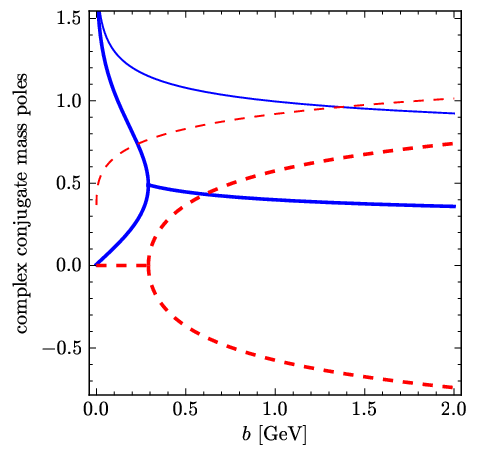
with a parameter . The quark propagator has then an infinite number of CCMPs, as exemplified on the left plot in Fig. 1. The position of the poles is controlled by the value of the gap. If the gap is larger than a critical value given by
| (32) |
all the poles are complex. For the quartet nearest to the origin, an especially interesting situation occurs. As the gap gets smaller, the poles travel to the real axis, where they meet in doublets at . If the gap is further reduced, , every doublet again splits, with one pole eventually going to plus (minus) infinity and the other arriving at (), for . At that point, the real parts of the higher quartets go to infinity, while the imaginary parts go to zero. See Fig. 1 for the behavior of the first and the second quartet w.r.t. the mass gap.
In our numerical calculations we adopt the parameters of Ref. [16], GeV, , and , successfully reproducing low-energy phenomenology. Here is the strength of the non-local effective gluon interaction (i.e., four-quark non-local NJL interaction). For these parameters one obtains GeV, while the vacuum solution of the gap equation is GeV. Thus, the gap is overcritical in this case.

III.2 Thermodynamic potential and in-medium mass gap
The in-medium properties of the model are obtained from the thermodynamic potential (1), coupled to the PL. In mean-field approximation (4) it is given by
| (33) |
see, e.g., [16]. Here and represents the mean-field PL potential, for which we use the familiar polynomial form found in Ref. [51]. Other forms of this potential are in use, like the logarithmic form [52], a strong-coupling inspired one [53] or a -dependent one [55]. For recent developments, see [56, 57, 58].
is provided by Eq. (7) augmented with the PL. This amounts to
| (34) |
where we now understand as diagonal matrices in color space
| (35) |
To simplify the calculations, a further restriction is imposed by setting , i.e., . The thermal properties of the model then follow from the minimization of the thermodynamic potential w.r.t. and . In particular, the and dependence of the dressing function is solely determined by the mass gap , as we have seen above. The explicit form of the mass gap equation is presented in the appendix.


In Fig. 2 the mass gap of a system without PL is shown as a function of the temperature along different lines of constant . The results of a full numerical solution (full lines) are compared with approximate ones where only a small number of poles is taken into account. The dotted lines indicate calculations where the system is approximated by only the lowest lying quartet, containing the states that become physical quark degrees of freedom when drops below . In order to demonstrate the convergence towards the full numerical results, we also show the effect of additionally including the second quartet (dashed lines).
An observation that will be crucial later on is that, at low temperatures, a perfect agreement with the numerical solutions is obtained already with the first quartet. Deviations start only after chiral restoration, so that at higher temperatures higher quartets are needed to develop the correct chiral behavior. In fact, for any finite number of poles, the mass gap increases again after reaching a minimum, so that the correct high-temperature limit is only reached if all poles are included.
As seen in Fig. 3, similar conclusions hold when the PL is introduced, although the deviations are slightly more pronounced after the chiral/deconfinement transition, and for higher chemical potential also around the transition. Let us observe that at (rightmost plot in Fig. 3), the system develops a first-order transition.


In Fig. 3 we also show the results for the PL expectation value. While the overall behavior is the expected one, rising from at low towards at high , it turns out that there is an intermediate regime below the cross-over temperature, where gets negative. Although formally allowed by the definition (17), which at the mean-field level boils down to , it is in sharp contrast to the standard interpretation of as exponential of the free energy of a static color source, [59]. We also note that, roughly in the same region, the gap parameter rises as a function of , a feature, which is even more pronounced in the calculation without PL, Fig. 2.
III.3 Pressure instabilities and instability suppression
To calculate the EoS, the kinetic contribution to the thermodynamic potential is regularized by subtracting the zero-point energy of free quarks, i.e.,
| (36) |
and the EoS is given by , where is a constant chosen to achieve zero pressure in the vacuum.
In Figs. 4 and 5, the pressure is displayed as a function of temperature, again along lines of constant . In the model without PL, the results are scaled by the pressure of noninteracting massless quarks,
| (37) |
whereas in the case with PL, we divide by the full Stefan-Boltzmann (SB) pressure of massless quarks and gluons,
| (38) |
The results for the model without PL are displayed in Fig. 4. The most striking features are the oscillations, which signal the thermodynamic instabilities, we have anticipated from the cosine terms in Eq. (16). They turn out to be particularly troublesome, as there are not only temperature regions where the pressure drops with increasing temperature, but where it gets even negative.** * Let us recall that we defined the vacuum pressure to be zero, so this result is clearly unphysical. Comparing the three panels of the figure, the results seem to be rather independent of the ratio . We should keep in mind, however, that the pressure is scaled by the SB value, which is larger for larger values of . Taking this into account, the instabilities grow with the chemical potential, since the Boltzmann factors are even less effective in damping the oscillating terms. This results in a rather large negative pressure for .
For comparison we show again the results obtained when we only take into account the lowest-lying poles. In agreement with our findings for the mass gap, we observe that, at low temperatures and more importantly, in the region of the instability, the pressure given by just the first quartet is an excellent approximation. The oscillations of the pressure can thus be understood quantitatively from the temperature dependence of shown in Fig. 2, together with the dependence of the lowest-lying poles shown in the right panel of Fig. 1. In particular, at around 150 MeV, the mass gap drops below , so that the lowest quartet splits into two real doublets and no longer yields an oscillating behavior.
At high temperatures, the full numerical result for the pressure (solid lines) approaches the SB limit, whereas the restriction to the first quartet (dotted) strongly overshoots this limit and is, thus, not a good approximation in this regime. The inclusion of the second quartet (dashed line) leads to some improvement but fails as well to reproduce the SB limit. This is consistent with Fig. 2, where the restriction to a few mass poles even qualitatively failed to reproduce the high-temperature behavior of the mass gap.
Introducing the PL leads to a dramatic improvement of the EoS. As demonstrated on Fig. 5, the oscillations are strongly suppressed. Since the PL does not eliminate all the cosine terms completely (see Eq. (21)), residual wiggles are still present on the results for , while at also a slightly negative pressure is observed in the full numerical calculation. We also note that the negative values of the PL, which we have seen in Fig. 3, appear roughly in the same temperature region, but are more pronounced at low chemical potentials. So, to some extent, there seems to be a trade-off between an unphysical behavior of the pressure and an unphysical behavior of the Polyakov loop (when interpreted as exponential of the free energy of a static quark).


III.4 Effect of the poles at
In the final part of this section, we want to discuss another consequence of the CCMPs, which shows up in the non-local chiral model at zero temperature. We recall that the PL decouples at and therefore has no effect in this case.
In the left panel of Fig. 6, we show the regularized thermodynamic potential as a function of the gap parameter for several values of the chemical potential . According to Eq. (27), the threshold chemical potential for non-zero quark number density is controlled by the lowest value of . Hence, at finite chemical potential, the thermodynamic potential has to stay at its vacuum value in those regions, where the lowest threshold, , is bigger than . This is similar to the local NJL model, where at the thermodynamic potential as a function of the constituent quark mass stays at its vacuum value for .†† † More general, this is a consequence of the so-called “Silver Blaze problem” [60], meaning that at the grand partition function must not change if is below the smallest excitation threshold. In the non-local model the essential difference is that the threshold is a non-monotonic function of the gap parameter . As we have seen in Fig. 1, it rises from at to a maximum at , where GeV for our parameters. Above this point, slowly decreases, reaching arbitrarily small values at large . As a consequence, for , the thermodynamic potential coincides with the vacuum curve only in a finite interval around , bounded by the condition . For the mass gap outside this range there is a finite density of quarks and the thermodynamic potential is below the vacuum one. An example for this case is given by the dashed line in the left panel of Fig. 6.
For the potential is reduced everywhere (dash-dotted line). Eventually, this leads to a pathological result: Whereas at intermediate chemical potentials a global minimum emerges near , leading to (approximate) chiral-symmetry restoration, at sufficiently high chemical potential, the nontrivial minimum at large becomes the global one, meaning that chiral symmetry is broken again (dotted line). The corresponding behavior of the gap parameter which minimizes the thermodynamic potential is shown in the middle of Fig. 6. This obviously unphysical result is a consequence of two facts: First, for there are two CCMPs, i.e., twice as many “degrees of freedom” which contribute to the pressure in the non-trivial minimum. Second, according to Eq. (26), the Fermi momentum is lowered by the real part but enhanced by the imaginary part of , and eventually becomes even larger than . These effects lead to a further enhancement of the density and thus the thermodynamic potential decreases faster in the non-trivial minimum than in the trivial one. This is also underlined by the right plot, where the pressure is displayed as a function of the chemical potential: In the second chirally broken phase, the immense rise in the density causes the EoS even to overshoot the pressure of a free quark gas.


The second breaking of chiral symmetry at high chemical potential is reminiscent to what we have found at high temperature, when we restricted ourselves to a finite number of poles, cf. Figs. 2 and 3. In fact, at , the chemical potential imposes a sharp cutoff on the thermal part of the thermodynamic potential, and in this sense, there is always only a finite number of poles which contribute. For instance, the highest value of considered considered in the left plot of Fig. 6 is still smaller than for the shown range of , and therefore the thermodynamics is determined completely by the first quartet.
IV Summary and conclusions
A realistic continuum effective theory of strongly interacting quarks and gluons should incorporate the two most striking features of low-energy QCD: chiral symmetry breaking and confinement. The first one represents a physically familiar concept, and it is rather easily modeled. The latter is still lacking a proper explanation, but can nevertheless be realized by various confining criteria like, e.g., positivity violation.
The simplest possible model of chiral quark dynamics is the Nambu–Jona-Lasinio model, exhibiting real mass poles, a feature shared with its nonlocal, but instantaneous generalizations. Although very successful, these models do not incorporate confinement. Models in which the quark propagator is an entire function represent the opposite situation that quasiparticle poles for quarks (and gluons) are absent, but therefore do not allow for deconfinement. In between, there is a large class of models that have poles in the complex plane, which, due to the their manifest covariance, come in complex conjugate pairs.
In this paper we have reported the observation that the thermodynamical state in such a class of models is unstable, due to the possibility of oscillating, or even negative, pressure. Further consequences can also be entropy decrease with the temperature or negative heat capacity, violating the standard stability criteria for thermodynamical equilibrium. This underlines that quark confinement is a multifaceted phenomenon that cannot exclusively be modeled as strong momentum dependence of dynamical mass and wave function renormalization. In this context we have investigated to what extent a suppression of these unphysical instabilities can be achieved by coupling the system to the Polyakov loop.
A simple quark model which reproduces the CCMP form of the quark propagator dynamically is a DSE model with a covariant separable interaction. As an example, we solved such a model for a Gaussian formfactor ansatz at finite temperature and chemical potential in mean-field approximation in order to demonstrate the possible effects of CCMPs on the thermodynamics. The results show that CCMPs are indeed the mechanism responsible for the instability. When coupling the quark propagator to the PL, we find that the pressure instabilities are strongly reduced. Unfortunately, more or less in the same region of the phase diagram, the PL itself becomes negative, which is in sharp contrast to its standard interpretation as exponential of the free energy of a static color source. Thus, although there is no exact one-to-one correspondence, it seems that one unphysical effect could only be suppressed to the expense of a new one.
At zero temperature and finite chemical potential the PL is irrelevant. For very high chemical potentials ( MeV in our case) CCMPs produce yet another unexpected and probably unphysical behavior: the chiral symmetry gets broken again.‡‡ ‡ At very high chemical potential chiral symmetry is expected to be broken again in a color-flavor locked phase [66], but this is a completely different mechanism. We expect, that the same behavior is persistent in a more realistic setup, i.e., when one includes the effects of wave function renormalization as, e.g., in [20, 21, 25].
From a wider perspective, vacuum instabilities in a mean-field (or “classical”) description of QCD are not uncommon; a prominent example being the tachyonic mode observed in the Savvidy vacuum [62, 63]. It is interesting to note that also in this case the PL acts as a “stabilizer”, i.e., by suppressing the original tachyonic modes [64, 65]. Unfortunately, this program is also not entirely successful as new unstable modes arise [64, 65].
Apparently, the lesson to be learnt is the following: in order to cure the thermodynamic instability problems in the low-temperature and low-density domain of effective “confining” models of quark (and /or gluon) matter properly one has to go beyond the mean-field level of description, however clever it may be designed. Only the explicit inclusion of the physical degrees of freedom in that domain, the hadrons as color neutral bound states of quarks and gluons, will provide the non-negative and monotonously rising pressure in the confinement domain of low-energy QCD. As first promising works in this direction we refer to [19, 21, 23, 26] and suggest to develop the CCMP propagator class models beyond mean field.
Acknowledgments
S.B. acknowledges discussions with D. Horvatić and G. Contrera as well as the hospitality of the University of Wroclaw where this work was started and completed. This work was supported by the Polish Ministry for Science and Higher Education and by CompStar, a Research Networking Programme of the European Science foundation. S.B. is also supported through the project No. 119-0982930-1016 of the Ministry of Science, Education and Sports of Croatia. D.B. acknowledges the kind hospitality during visits at the Institut für Kernphysik of Technische Universität Darmstadt as well as support by the Polish National Science Center (NCN) under grant no. NN 202 231837 and by the Russian Fund for Basic Research under grant no. 11-02-01538-a. M.B. thanks D.B. for his kind hospitality at the University of Rostock and at ECT∗ in Trento where initial work for this paper was done more than a decade ago.
Appendix A Gap equation in medium
This appendix presents the quark gap equation in the mean-field approximation, with the Matsubara summation being analytically performed.
Minimizing the mean-field thermodynamic potential (33), the quark gap at is obtained to be
| (39) |
where is to be understood as a diagonal color matrix, see (35). The sum over Matsubara frequencies is evaluated using the standard technique of rewriting it as the sum over residues of a contour integral in the complex energy plane over the analytically continued integrand function folded with the function (18) having simple poles at the PL shifted Matsubara frequencies. The Matsubara summation is thus converted into three closed contour integrals, similar to what was performed in Sec. II. These are calculated by the residue theorem, giving the result
| (40) |
The first term is recognized as the vacuum gap equation. Residues can easily be deduced to be
| (41) |
with given by (10) when . An expression for a color trace of the occupation numbers
| (42) |
completes the calculation.
References
- [1] Y. Aoki, S. Borsanyi, S. Dürr, Z. Fodor, S. D. Katz, S. Krieg and K. K. Szabo, JHEP 0906, 088 (2009).
- [2] S. Borsanyi, Z. Fodor, C. Hoelbling, S. D. Katz, S. Krieg, C. Ratti and K. K. Szabo, JHEP 1009, 073 (2010).
- [3] S. Borsanyi et al., JHEP 1011, 077 (2010).
- [4] M. Cheng et al., Phys. Rev. D 81, 054504 (2010).
- [5] A. Bazavov and P. Petreczky, J. Phys. Conf. Ser. 230, 012014 (2010).
- [6] A. Bazavov and P. Petreczky, PoS LATTICE2010, 215 (2010).
- [7] A. Bazavov and P. Petreczky, PoS LATTICE2010, 169 (2010).
- [8] W. Söldner [HotQCD collaboration], PoS LATTICE2010, 215 (2010).
- [9] C. D. Roberts and S. M. Schmidt, Prog. Part. Nucl. Phys. 45 (2000) S1.
- [10] R. Alkofer and L. von Smekal, Phys. Rept. 353 (2001) 281.
- [11] C. S. Fischer, J. Phys. G 32, R253 (2006).
- [12] R. S. Plant and M. C. Birse, Nucl. Phys. A 628 (1998) 607.
- [13] I. General, D. Gomez Dumm and N. N. Scoccola, Phys. Lett. B 506 (2001) 267.
- [14] D. Gomez Dumm and N. N. Scoccola, Phys. Rev. D 65 (2002) 074021.
- [15] D. Gomez Dumm and N. N. Scoccola, Phys. Rev. C 72 (2005) 014909.
- [16] D. Blaschke and P. C. Tandy, In *Trento 1999, Understanding deconfinement in QCD* 218-230 [nucl-th/9905067].
- [17] D. Blaschke, G. Burau, Y. .L. Kalinovsky, P. Maris and P. C. Tandy, Int. J. Mod. Phys. A 16 (2001) 2267.
- [18] D. Blaschke, D. Horvatic, D. Klabucar and A. E. Radzhabov, hep-ph/0703188 [HEP-PH].
- [19] D. Blaschke, M. Buballa, A. E. Radzhabov and M. K. Volkov, Yad. Fiz. 71 (2008) 2012 [Phys. Atom. Nucl. 71 (2008) 1981].
- [20] G. A. Contrera, D. Gomez Dumm and N. N. Scoccola, Phys. Lett. B 661 (2008) 113.
- [21] T. Hell, S. Roessner, M. Cristoforetti and W. Weise, Phys. Rev. D 79 (2009) 014022.
- [22] S. Noguera and N. N. Scoccola, Phys. Rev. D 78, 114002 (2008).
- [23] T. Hell, S. Rossner, M. Cristoforetti and W. Weise, Phys. Rev. D 81, 074034 (2010).
- [24] G. A. Contrera, M. Orsaria and N. N. Scoccola, Phys. Rev. D 82 (2010) 054026.
- [25] D. Horvatic, D. Blaschke, D. Klabucar and O. Kaczmarek, Phys. Rev. D 84 (2011) 016005.
- [26] A. E. Radzhabov, D. Blaschke, M. Buballa and M. K. Volkov, Phys. Rev. D 83, 116004 (2011).
- [27] G. Krein, C. D. Roberts and A. G. Williams, Int. J. Mod. Phys. A 7 (1992) 5607.
- [28] C. J. Burden, C. D. Roberts and A. G. Williams, Phys. Lett. B 285 (1992) 347.
- [29] S. J. Stainsby and R. T. Cahill, Int. J. Mod. Phys. A 7 (1992) 7541.
- [30] C. J. Burden, Phys. Rev. D 57 (1998) 276.
- [31] V. N. Gribov, Eur. Phys. J. C 10 (1999) 91.
- [32] R. Alkofer, W. Detmold, C. S. Fischer and P. Maris, Phys. Rev. D 70 (2004) 014014.
- [33] M. Buballa and S. Krewald, Phys. Lett. B 294 (1992) 19.
- [34] H. J. Munczek and A. M. Nemirovsky, Phys. Rev. D 28, 181 (1983).
- [35] G. V. Efimov and S. N. Nedelko, Phys. Rev. D 51 (1995) 176.
- [36] M. S. Bhagwat, M. A. Pichowsky, C. D. Roberts and P. C. Tandy, Phys. Rev. C 68 (2003) 015203.
- [37] H. Chen, W. Yuan, L. Chang, Y. -X. Liu, T. Klähn and C. D. Roberts, Phys. Rev. D 78 (2008) 116015.
- [38] B. C. Tiburzi, W. Detmold and G. A. Miller, Phys. Rev. D 68 (2003) 073002.
- [39] M. Bhagwat, M. A. Pichowsky and P. C. Tandy, Phys. Rev. D 67 (2003) 054019.
- [40] A. Scarpettini, D. Gomez Dumm and N. N. Scoccola, Phys. Rev. D 69 (2004) 114018.
- [41] J. M. Cornwall, R. Jackiw and E. Tomboulis, Phys. Rev. D 10 (1974) 2428.
- [42] Y. Nambu and G. Jona-Lasinio, Phys. Rev. 122 (1961) 345.
- [43] Y. Nambu and G. Jona-Lasinio, Phys. Rev. 124 (1961) 246.
- [44] S. Klimt, M. Lutz, U. Vogl and W. Weise, Nucl. Phys. A 516, 429 (1990); Nucl. Phys. A 516, 469 (1990).
- [45] S. P. Klevansky, Rev. Mod. Phys. 64, 649 (1992).
- [46] T. Hatsuda and T. Kunihiro, Phys. Rept. 247, 221 (1994).
- [47] M. Buballa, Phys. Rept. 407, 205 (2005).
- [48] A. M. Polyakov, Phys. Lett. B 72 (1978) 477.
- [49] P. N. Meisinger and M. C. Ogilvie, Phys. Lett. B 379 (1996) 163.
- [50] K. Fukushima, Phys. Lett. B 591, 277 (2004).
- [51] C. Ratti, M. A. Thaler and W. Weise, Phys. Rev. D 73 (2006) 014019.
- [52] S. Roessner, C. Ratti and W. Weise, Phys. Rev. D 75, 034007 (2007).
- [53] K. Fukushima, Phys. Rev. D 77, 114028 (2008) [Erratum-ibid. D 78, 039902 (2008)].
- [54] M. Loewe, P. Morales and C. Villavicencio, Phys. Rev. D 83 (2011) 096005.
- [55] V. A. Dexheimer and S. Schramm, Nucl. Phys. Proc. Suppl. 199, 319 (2010).
- [56] C. Sasaki and K. Redlich, arXiv:1204.4330 [hep-ph].
- [57] M. Ruggieri, P. Alba, P. Castorina, S. Plumari, C. Ratti and V. Greco, arXiv:1204.5995 [hep-ph].
- [58] K. Fukushima and K. Kashiwa, arXiv:1206.0685 [hep-ph].
- [59] L. D. McLerran and B. Svetitsky, Phys. Rev. D 24, 450 (1981).
- [60] T. D. Cohen, Phys. Rev. Lett. 91, 222001 (2003).
- [61] S. M. Schmidt, D. Blaschke and Y. .L. Kalinovsky, Phys. Rev. C 50 (1994) 435.
- [62] G. K. Savvidy, Phys. Lett. B 71 (1977) 133.
- [63] N. K. Nielsen and P. Olesen, Nucl. Phys. B 144 (1978) 376.
- [64] P. N. Meisinger and M. C. Ogilvie, Phys. Lett. B 407 (1997) 297.
- [65] P. N. Meisinger and M. C. Ogilvie, Phys. Rev. D 66 (2002) 105006.
- [66] M. G. Alford, K. Rajagopal and F. Wilczek, Nucl. Phys. B 537, 443 (1999)