A comparison of the discrete Kolmogorov-Smirnov statistic and the Euclidean distance
Abstract
Goodness-of-fit tests gauge whether a given set of observations is consistent (up to expected random fluctuations) with arising as independent and identically distributed (i.i.d.) draws from a user-specified probability distribution known as the “model.” The standard gauges involve the discrepancy between the model and the empirical distribution of the observed draws. Some measures of discrepancy are cumulative; others are not. The most popular cumulative measure is the Kolmogorov-Smirnov statistic; when all probability distributions under consideration are discrete, a natural noncumulative measure is the Euclidean distance between the model and the empirical distributions. In the present paper, both mathematical analysis and its illustration via various data sets indicate that the Kolmogorov-Smirnov statistic tends to be more powerful than the Euclidean distance when there is a natural ordering for the values that the draws can take — that is, when the data is ordinal — whereas the Euclidean distance is more reliable and more easily understood than the Kolmogorov-Smirnov statistic when there is no natural ordering (or partial order) — that is, when the data is nominal.
Keywords: significance, hypothesis, chi-square, root-mean-square, mean-square
1 Introduction
Testing goodness-of-fit is one of the foundations of modern statistics, as elucidated by Rao (2002), for example. The formulation in the discrete setting involves independent and identically distributed (i.i.d.) draws from a probability distribution over bins (“categories,” “cells,” and “classes” are common synonyms for “bins”). In accordance with the standard conventions, we will use to denote the actual (unknown) underlying distribution of the draws; , with , , …, being nonnegative and
| (1) |
We will use to denote a user-specified distribution, usually called the “model”; again , with , , …, being nonnegative and
| (2) |
A goodness-of-fit test produces a value — the “P-value” — that gauges the consistency of the observed data with the assumption that . In many formulations, the user-specified model consists of a family of probability distributions parameterized by , where can be integer-valued, real-valued, complex-valued, vector-valued, matrix-valued, or any combination of the many possibilities. In such cases, the P-value gauges the consistency of the observed data with the assumption that , where is an estimate (taken to be the maximum-likelihood estimate throughout the present paper). We now review the definition of P-values.
P-values are defined via the empirical distribution , where , with being the proportion of the observed draws that fall in the th bin, that is, is the number of draws falling in the th bin, divided by . P-values involve a hypothetical experiment taking i.i.d. draws from the assumed actual underlying distribution . We denote by the empirical distribution of the draws from the hypothetical experiment; we denote by a maximum-likelihood estimate of obtained from the hypothetical experiment. The P-value is then the probability that the discrepancy between the random variables and is at least as large as the observed discrepancy between and , calculating the probability under the assumption that .
To complete the definition of P-values, we must choose a measure of discrepancy. In the present paper, we consider the (discrete) Kolmogorov-Smirnov and Euclidean distances,
| (3) |
and
| (4) |
respectively. The P-value for the Kolmogorov-Smirnov statistic is the probability that ; the P-value for the Euclidean distance is the probability that . When evaluating the probabilities, we view and as random variables, constructed with i.i.d. draws from the assumed distribution , while viewing the observed and as fixed, not random.
If a P-value is very small, then we can be confident that the given observed draws are inconsistent with the assumed model, are not i.i.d., or are both inconsistent and not i.i.d.
Needless to say, the Kolmogorov-Smirnov distance defined in (3) is the maximum absolute difference between cumulative distribution functions. The Kolmogorov-Smirnov statistic depends on the ordering of the bins, unlike the Euclidean distance.
As supported by the investigations below, we recommend using the Kolmogorov-Smirnov statistic when there is a natural ordering of the bins, while the Euclidean distance is more reliable and more easily understood than the Kolmogorov-Smirnov statistic when there is no natural ordering (or partial order). Unlike the Euclidean distance, the Kolmogorov-Smirnov statistic utilizes the information in a natural ordering of the bins, when the latter is available. Horn (1977) gave similar recommendations when comparing the and Kolmogorov-Smirnov statistics. Detailed comparisons between the Euclidean distance and statistics are available in Perkins et al. (2011a).
The Kolmogorov-Smirnov statistic is cumulative; it accentuates low-frequency differences between the model and the empirical distribution of the draws, but tends to average away and otherwise obscure high-frequency differences. Similar observations have been made by Pettitt and Stephens (1977), D’Agostino and Stephens (1986), Choulakian et al. (1994), From (1996), Best and Rayner (1997), Haschenburger and Spinelli (2005), Steele and Chaseling (2006), Lockhart et al. (2007), Ampadu (2008), and Ampadu et al. (2009), among others. Our suggestions appear to be closest to those of Horn (1977).
There are many cumulative approaches similar to the Kolmogorov-Smirnov statistic. These include the Cramér–von-Mises, Watson, Kuiper, and Rényi statistics, as well as their Anderson-Darling variants; Section 14.3.4 of Press et al. (2007), Stephens (1970), and Rényi (1953) review these statistics. We ourselves are fond of the Kuiper approach. However, the present paper focuses on the popular Kolmogorov-Smirnov statistic; the Cramér–von-Mises, Watson, and Kuiper variants are very similar.
The remainder of the present paper has the following structure: Section 2 describes how the Euclidean distance is generally preferable to the Kolmogorov-Smirnov statistic when there is no natural ordering (or partial order) of the bins. Section 3 describes how the Kolmogorov-Smirnov statistic is generally preferable to the Euclidean distance when there is a natural ordering of the bins. Section 4 illustrates both cases with examples of data sets and the associated P-values, computing the P-values via Monte-Carlo simulations with guaranteed error bounds. The reader may wish to begin with Section 4, referring back to earlier sections as needed.
2 The case when the bins do not have a natural order
The Euclidean distance is generally preferable to the Kolmogorov-Smirnov statistic when there is no natural ordering (or partial order) of the bins. As discussed by Perkins et al. (2011b), the interaction of parameter estimation and the Euclidean distance is easy to understand and quantify, at least asymptotically, in the limit of large numbers of draws. In contrast, the interaction of parameter estimation and the Kolmogorov-Smirnov statistic can be very complicated, though Choulakian et al. (1994) and Lockhart et al. (2007) have pointed out that the interaction is somewhat simpler with Cramér’s and von Mises’, Watson’s, and some of Anderson’s and Darling’s very similar statistics. That said, the Euclidean distance can be more reliable even when there are no parameters in the model, that is, when the model is a single, fixed, fully specified probability distribution; the remainder of the present section describes why.
The basis of the analysis is the following lemma, a reformulation of the fact that the expected maximum absolute deviation from zero of the standard Brownian bridge is (Marsaglia et al., 2003, see, for example, Section 3 of).
Lemma 2.1.
Suppose that is even and that , , …, form a randomly ordered list of positive ones and negative ones (with the ordering drawn uniformly at random). Then,
| (5) |
in the limit that , where (as usual) produces the expected value.
We denote by the actual underlying distribution of the observed i.i.d. draws. We denote by the model distribution. We denote by the empirical distribution of the draws. These are all probability distributions, that is, , , and for , , …, , and (1) and (2) hold.
Suppose that the actual underlying distribution , , …, of the draws is the same as the model distribution , , …, ; the random variables , , …, are then the proportions of i.i.d. draws from that fall in the respective bins. The Euclidean distance is
| (6) |
The Kolmogorov-Smirnov statistic is
| (7) |
The expected value of the square of the Euclidean distance is
| (8) |
As shown, for example, by Durbin (1972) using Lemma 2.1 above, the expected value of times the Kolmogorov-Smirnov statistic is
| (9) |
in the limit that and . Comparing (8) and (9), we see that and are roughly the same size (inversely proportional to ) when the actual underlying distribution of the draws is the same as the model distribution.
However, when the actual underlying distribution of the draws differs from the model distribution, the Euclidean distance and the Kolmogorov-Smirnov statistic can be very different. If the number of draws is large, then the empirical distribution will be very close to the actual distribution . Therefore, to study the performance of the goodness-of-fit statistics as when the actual distribution differs from the model distribution (and both are independent of ), we can focus on the difference between and (rather than the difference between and ). We now define and study the difference
| (10) |
for , , …, . The Euclidean distance between and (the root-sum-square difference) is
| (11) |
The Kolmogorov-Smirnov statistic (the maximum absolute cumulative difference) is
| (12) |
For simplicity (and because the following analysis generalizes straightforwardly), let us consider the illustrative case in which , that is,
| (13) |
for all , , …, , where is a positive real number ( must always satisfy , since ). Combining (10), (1), and (2) yields that
| (14) |
Together, (14) and (13) imply that is even and that half of , , …, are equal to , and the other half are equal to .
Combining (13) and (11) yields that the Euclidean distance is
| (15) |
The fact that half of , , …, are equal to , and the other half are equal to , yields that the Kolmogorov-Smirnov statistic defined in (12) could be as small as or as large as , depending on the ordering of the signs in , , …, . If all orderings are equally likely (which is equivalent to ordering the bins uniformly at random), then by Lemma 2.1 the mean value for is in the limit that is large (this is the expected maximum absolute deviation from zero of a tied-down random walk with steps, each of length , that starts and ends at zero; the random walk ends at zero due to (14)).
Thus, in the limit that the number of draws is large (and , while both the model and the alternative distribution are independent of ), the Euclidean distance and the Kolmogorov-Smirnov statistic have similar statistical power on average, if all orderings of the bins are equally likely. However, the Euclidean distance is the same for any ordering of the bins, whereas the power of the Kolmogorov-Smirnov statistic depends strongly on the ordering. We see, then, that the Euclidean distance is more reliable than the Kolmogorov-Smirnov statistic when there is no especially natural ordering for the bins.
Remark 2.2.
It is possible to use an ordering for which the Kolmogorov-Smirnov statistic attains its greatest value (this corresponds to renumbering the bins such that the differences satisfy or ). However, this data-dependent ordering produces a statistic which is proportional to the distance (whereas the Euclidean distance is the distance), as remarked at the top of page 396 of Hoeffding (1965). The resulting statistic is no longer cumulative.
3 The case when the bins have a natural order
The Kolmogorov-Smirnov statistic is often preferable to the Euclidean distance when there is a natural ordering of the bins. In fact, the Kolmogorov-Smirnov statistic is always preferable when the data is very sparse and there is a natural ordering of the bins. In the limit that the maximum expected number of draws per bin tends to zero, the Euclidean distance always takes the same value under the null hypothesis, providing no discriminative power: indeed, when the draws producing the empirical distribution are taken from the model distribution , the Euclidean distance is almost surely ,
| (16) |
in the limit that (the reason is that, in this limit, and moreover almost every realization of the experiment satisfies that, for all , , …, , or , that is, there is at most one observed draw per bin). In contrast, the Kolmogorov-Smirnov statistic is nontrivial even in the limit that the maximum expected number of draws per bin tends to zero — in fact, this is exactly the continuum limit for the original Kolmogorov-Smirnov statistic involving continuous cumulative distribution functions (as opposed to the discontinuous cumulative distribution functions arising from the discrete distributions considered in the present paper). Furthermore, the Kolmogorov-Smirnov statistic is sensitive to symmetry (or asymmetry) in a distribution, and can detect other interesting properties of distributions that depend on the ordering of the bins.
4 Data analysis
This section gives four examples illustrating the performance of the Kolmogorov-Smirnov statistic and the Euclidean distance in various circumstances. The Kolmogorov-Smirnov statistic is more powerful than the Euclidean distance in the first two examples, for which there are natural orderings of the bins. The Euclidean distance is more reliable than the Kolmogorov-Smirnov statistic in the last two examples, for which any ordering of the bins is necessarily rather arbitrary. We computed all P-values via Monte-Carlo simulations with guaranteed error bounds, as in Remark 3.3 of Perkins et al. (2011a). Remark 3.4 of Perkins et al. (2011a) proves that the standard error of the estimate for a P-value is , where is the number of simulations conducted to calculate the P-value.
4.1 A test of randomness
A particular random number generator is supposed to produce an integer from 1 to uniformly at random. The model distribution for such a generator is
| (17) |
for , , …, . We test the (obviously poor) generator which produces the numbers 1, 2, 3, …, , in that order, so that the observed distribution of the generated numbers is
| (18) |
for , , …, . For these observations, the P-value for the Euclidean distance is 1 to several digits of precision, while the P-value for the Kolmogorov-Smirnov statistic is 0 to several digits, at least for between a hundred and a million. So, as expected, the Euclidean distance has almost no discriminative power for such sparse data, whereas the Kolmogorov-Smirnov statistic easily discerns that the data (18) is inconsistent with the model (17).
Remark 4.1.
Like the Euclidean distance, classical goodness-of-fit statistics such as , (the log–likelihood-ratio), and the Freeman-Tukey/Hellinger distance are invariant to the ordering of the bins, and also produce P-values that are equal to 1 to several digits of precision, at least for between a hundred and a million. For definitions and further discussion of the , , and Freeman-Tukey statistics, see Section 2 of Perkins et al. (2011a).
4.2 A test of Poissonity
A Poisson-distributed random number generator with mean is supposed to produce a nonnegative integer according to the model
| (19) |
for , , , , …. We test the (obviously poor) generator which produces the numbers 100, 101, 102, …, 109, so that the observed distribution of the numbers is
| (20) |
for , , , , …. The P-values, each computed via 4,000,000 simulations, are
- •
Kolmogorov-Smirnov: .0075
- •
Euclidean distance: .998
- •
: .999
- •
(the log–likelihood-ratio): .999
- •
Freeman-Tukey (the Hellinger distance): .998
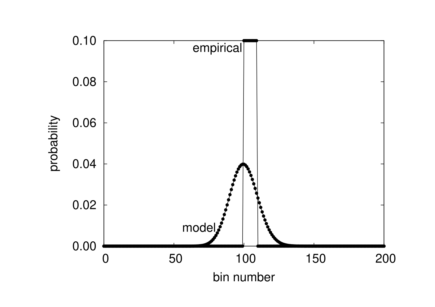
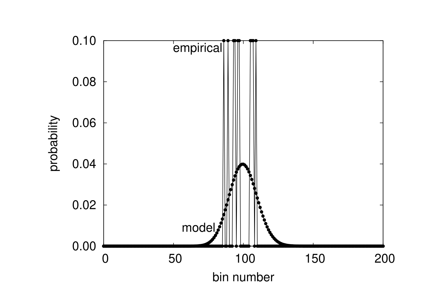
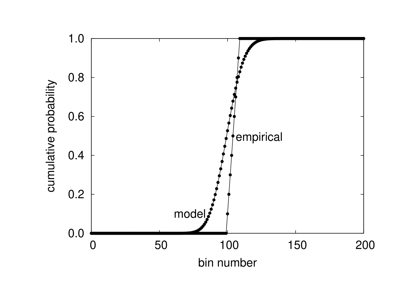
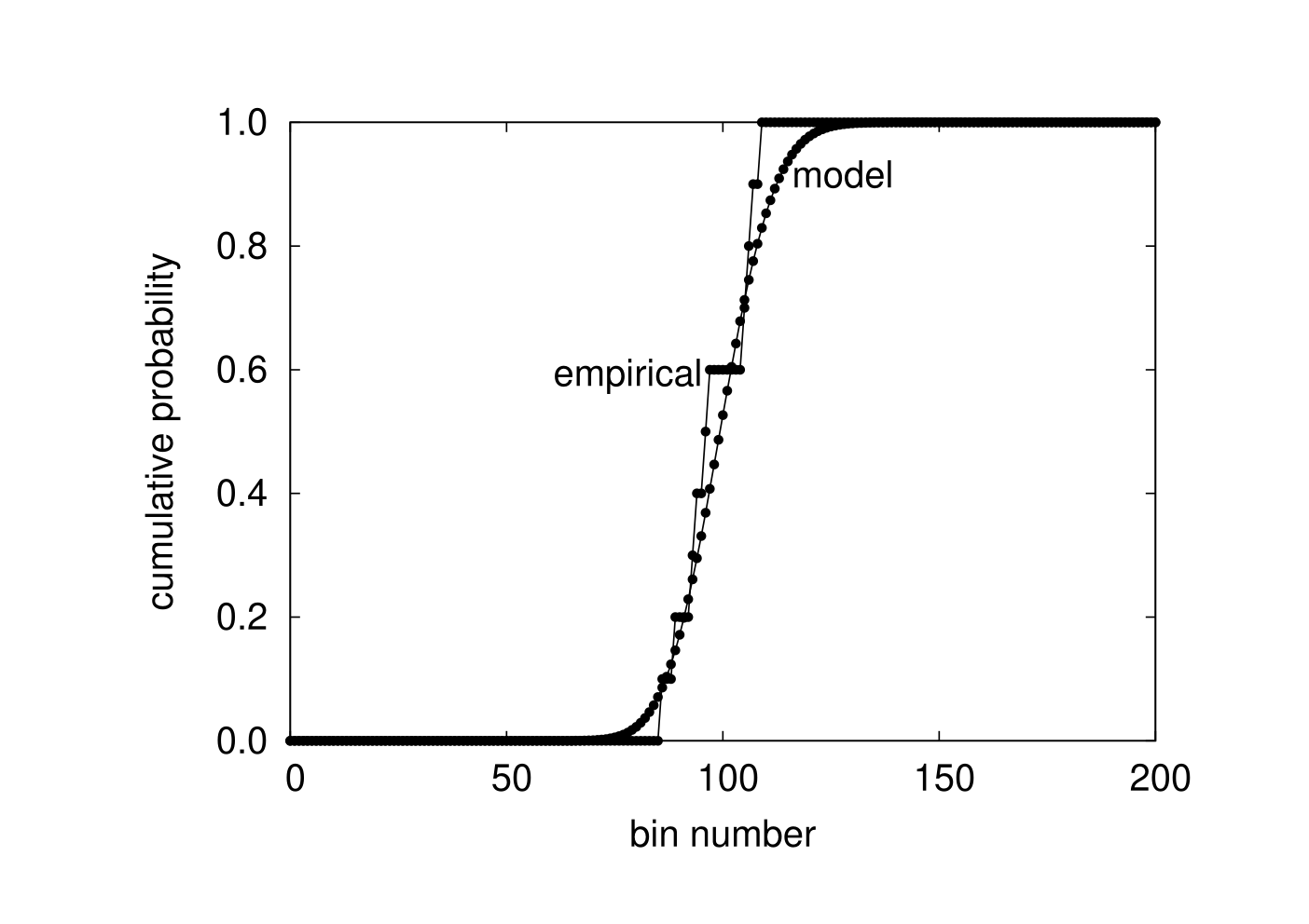
For definitions and further discussion of the , , and Freeman-Tukey statistics, see Section 2 of Perkins et al. (2011a). The Kolmogorov-Smirnov statistic is far more powerful for this example, in which the bins have a natural ordering (in this example the bins are the nonnegative integers).
Figure 1 plots the model probabilities , , , … defined in (19) along with the observed proportions , , , … defined in (20). Figure 2 plots the model probabilities , , , … along with analogues of the proportions , , , … for a simulation generating 10 i.i.d. draws according to the model.
Figure 3 plots the cumulative model probabilities , , , … along with the cumulative observed proportions , , , …. Figure 4 plots the cumulative model probabilities , , , … along with analogues of the cumulative proportions , , , … for the simulation generating 10 i.i.d. draws according to the model.
4.3 A test of Hardy-Weinberg equilibrium
In a population with suitably random mating, the proportions of pairs of Rhesus haplotypes in members of the population (each member has one pair) can be expected to follow the Hardy-Weinberg law discussed by Guo and Thompson (1992), namely to arise via random sampling from the model
| (21) |
for , , …, with , under the constraint that
| (22) |
where the parameters , , …, are the proportions of the nine Rhesus haplotypes in the population (naturally, their maximum-likelihood estimates are the proportions of the haplotypes in the given data). For , , …, with , therefore, is the expected probability that the pair of haplotypes in the genome of an individual is the pair and , given the parameters , , …, .
In this formulation, the hypothesis of suitably random mating entails that the members of the sample population are i.i.d. draws from the model specified in (21); if a goodness-of-fit statistic rejects the model with high confidence, then we can be confident that mating has not been suitably random.
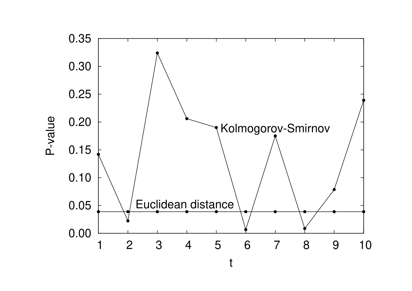
Table 1 provides data on individuals; we duplicated Figure 3 of Guo and Thompson (1992) to obtain Table 1. Figure 5 plots the associated P-values, each computed via 90,000 Monte-Carlo simulations. The Kolmogorov-Smirnov statistic depends on the ordering of the bins; for the first trial in Figure 5, the order of the bins is the lexicographical ordering, namely , , , , , , …, . The nine trials , , …, displayed in Figure 5 use pseudorandom orderings of the bins. Please note that the Euclidean distance does not depend on the ordering.
Generally, a more powerful statistic produces lower P-values. In Figure 5, the P-values for the Kolmogorov-Smirnov statistic are sometimes lower, sometimes higher than the P-values for the Euclidean distance. There is no particularly natural ordering of the bins for Figure 5; Figure 5 displays 10 different orderings corresponding to 10 different trials. Figure 5 demonstrates that the Euclidean distance is more reliable than the Kolmogorov-Smirnov statistic when there is no natural ordering (or partial order) for the bins.
Remark 4.2.
The P-values for classical goodness-of-fit statistics are substantially higher; the classical statistics are less powerful for this example. The P-values, each computed via 4,000,000 Monte-Carlo simulations, are
- •
Euclidean distance: .039
- •
: .693
- •
(the log–likelihood-ratio): .600
- •
Freeman-Tukey (the Hellinger distance): .562
For definitions and further discussion of the , , and Freeman-Tukey statistics, see Section 4.5 of Perkins et al. (2011a). Like the Euclidean distance, the , , and Freeman-Tukey statistics are all invariant to the ordering of the bins.
1 2 3 4 5 6 7 8 9 1 1236 2 120 3 3 18 0 0 4 982 55 7 249 5 32 1 0 12 0 6 2582 132 20 1162 29 1312 7 6 0 0 4 0 4 0 8 2 0 0 0 0 0 0 0 9 115 5 2 53 1 149 0 0 4
4.4 A test of uniformity
Table 2 duplicates Table 1 of Gilchrist (2010), giving the colors of the pieces of candy in a 2.17 ounce bag. Figure 6 plots the P-values for Table 2 to be consistent up to expected random fluctuations with Table 3, the model of uniform proportions. We computed each P-value via 4,000,000 Monte-Carlo simulations. The Kolmogorov-Smirnov statistic depends on the ordering of the bins; the ten trials , , …, displayed in Figure 6 use pseudorandom orderings of the bins. The Euclidean distance does not depend on the ordering.
Generally, a more powerful statistic produces lower P-values. In Figure 6, the P-values for the Kolmogorov-Smirnov statistic are sometimes lower, sometimes higher than the P-values for the Euclidean distance. There is no particularly natural ordering of the bins for Table 3; Figure 6 displays 10 different pseudorandom orderings corresponding to 10 different trials. Figure 6 illustrates that the Euclidean distance is more reliable than the Kolmogorov-Smirnov statistic when there is no natural ordering (or partial order) for the bins.
Remark 4.3.
Remark 4.4.
Like the Euclidean distance, many classical goodness-of-fit statistics are invariant to the ordering of the bins. The following are P-values, each computed via 4,000,000 Monte-Carlo simulations:
- •
Euclidean distance: .770
- •
: .770
- •
(the log–likelihood-ratio): .766
- •
Freeman-Tukey (the Hellinger distance): .755
For definitions and further discussion of the , , and Freeman-Tukey statistics, see Section 2 of Perkins et al. (2011a). For this example, the Euclidean distance and the statistic produce exactly the same P-values: for the model of homogeneous proportions, displayed in Table 3, the Euclidean distance is directly proportional to the square root of the statistic, and hence the Euclidean distance is a strictly increasing function of .
| color | red | orange | yellow | green | violet | |
|---|---|---|---|---|---|---|
| number | 15 | 9 | 14 | 11 | 13 |
| color | red | orange | yellow | green | violet | |
|---|---|---|---|---|---|---|
| number | 12.4 | 12.4 | 12.4 | 12.4 | 12.4 |

Acknowledgements
We would like to thank Alex Barnett, Gérard Ben Arous, James Berger, Tony Cai, Sourav Chatterjee, Ronald Raphael Coifman, Ingrid Daubechies, Jianqing Fan, Jiayang Gao, Andrew Gelman, Leslie Greengard, Peter W. Jones, Deborah Mayo, Peter McCullagh, Michael O’Neil, Ron Peled, William Perkins, William H. Press, Vladimir Rokhlin, Joseph Romano, Gary Simon, Amit Singer, Michael Stein, Stephen Stigler, Joel Tropp, Larry Wasserman, and Douglas A. Wolfe. This work was supported in part by Alfred P. Sloan Research Fellowships, a Donald D. Harrington Faculty Fellowship, and a DARPA Young Faculty Award.
References
- Ampadu (2008) Ampadu, C. (2008), On the powers of some new chi-square type statistics, Far East J. Theoretical Statist., 26, 59–72.
- Ampadu et al. (2009) Ampadu, C., Wang, D., and Steele, M. (2009), Simulated power of some discrete goodness-of-fit test statistics for testing the null hypothesis of a zig-zag distribution, Far East J. Theoretical Statist., 28, 157–171.
- Best and Rayner (1997) Best, D. J. and Rayner, J. C. W. (1997), Goodness-of-fit for the ordered categories discrete uniform distribution, Comm. Statist. Theory Meth., 26, 899–909.
- Choulakian et al. (1994) Choulakian, V., Lockhart, R. A., and Stephens, M. A. (1994), Cramér–von-Mises statistics for discrete distributions, Canadian J. Statist., 22, 125–137.
- D’Agostino and Stephens (1986) D’Agostino, R. B. and Stephens, M. A. (1986), Goodness-of-Fit Techniques, New York: Marcel Dekker.
- Durbin (1972) Durbin, J. (1972), Distribution Theory for Tests Based on the Sample Distribution Function, CBMS-NSF Regional Conference Series in Applied Mathematics, Philadelphia: Society for Industrial and Applied Mathematics.
- From (1996) From, S. G. (1996), A new goodness-of-fit test for the equality of multinomial cell probabilities versus trend alternatives, Comm. Statist. Theory Meth., 25, 3167–3183.
- Gilchrist (2010) Gilchrist, E. (2010), A sweet approach to teaching the one-variable chi-square test, Communication Teacher, 24, 14–18.
- Guo and Thompson (1992) Guo, S. W. and Thompson, E. A. (1992), Performing the exact test of Hardy-Weinberg proportion for multiple alleles, Biometrics, 48, 361–372.
- Haschenburger and Spinelli (2005) Haschenburger, J. K. and Spinelli, J. J. (2005), Assessing the goodness-of-fit of statistical distributions when data are grouped, Math. Geology, 37, 261–276.
- Hoeffding (1965) Hoeffding, W. (1965), Asymptotically optimal tests for multinomial distributions, Ann. Math. Statist., 36, 369–401.
- Horn (1977) Horn, S. D. (1977), Goodness-of-fit tests for discrete data: a review and an application to a health impairment scale, Biometrics, 33, 237–247.
- Lockhart et al. (2007) Lockhart, R. A., Spinelli, J. J., and Stephens, M. A. (2007), Cramér–von-Mises statistics for discrete distributions with unknown parameters, Canadian J. Statist., 35, 125–133.
- Marsaglia et al. (2003) Marsaglia, G., Tsang, W. W., and Wang, J. (2003), Evaluating Kolmogorov’s distribution, J. Statist. Soft., 8, 1–4.
- Perkins et al. (2011a) Perkins, W., Tygert, M., and Ward, R. (2011a), and classical exact tests often wildly misreport significance; the remedy lies in computers, Tech. Rep. 1108.4126, arXiv, http://cims.nyu.edu/tygert/abbreviated.pdf.
- Perkins et al. (2011b) Perkins, W., Tygert, M., and Ward, R. (2011b), Computing the confidence levels for a root-mean-square test of goodness-of-fit, II, Tech. Rep. 1009.2260, arXiv.
- Pettitt and Stephens (1977) Pettitt, A. N. and Stephens, M. A. (1977), The Kolmogorov-Smirnov goodness-of-fit statistic with discrete and grouped data, Technometrics, 19, 205–210.
- Press et al. (2007) Press, W., Teukolsky, S., Vetterling, W., and Flannery, B. (2007), Numerical Recipes, Cambridge, UK: Cambridge University Press, 3rd ed.
- Rao (2002) Rao, C. R. (2002), Karl Pearson chi-square test: The dawn of statistical inference, In Goodness-of-Fit Tests and Model Validity (eds Huber-Carol, C., Balakrishnan, N., Nikulin, M. S., and Mesbah, M.), pp. 9–24, Boston: Birkhäuser.
- Rényi (1953) Rényi, A. (1953), On the theory of order statistics, Acta Math. Acad. Sci. Hungar., 4, 191–231.
- Steele and Chaseling (2006) Steele, M. and Chaseling, J. (2006), Powers of discrete goodness-of-fit statistics for a uniform null against a selection of alternative distributions, Comm. Statist. Simul. Comput., 35, 1067–1075.
- Stephens (1970) Stephens, M. A. (1970), Use of the Kolmogorov-Smirnov, Cramér–Von-Mises and related statistics without extensive tables, J. Roy. Statist. Soc. Ser. B, 32, 115–122.