On the Spectral Lags and Peak-Counts of the
Gamma-Ray
Bursts Detected by the RHESSI Satellite
Abstract
A sample of 427 gamma-ray bursts from a database (February 2002 - April 2008) of the RHESSI satellite is analyzed statistically. The spectral lags and peak-count rates, which have been calculated for the first time in this paper, are studied completing an earlier analysis of durations and hardness ratios. The analysis of the RHESSI database has already inferred the existence of a third group with intermediate duration, apart from the so-called short and long groups. First aim of this article is to discuss the properties of these intermediate-duration bursts in terms of peak-count rates and spectral lags. Second aim is to discuss the number of GRB groups using another statistical method and by employing the peak-count rates and spectral lags as well. The standard parametric (model-based clustering) and non-parametric (K-means clustering) statistical tests together with the Kolmogorov-Smirnov and Anderson-Darling tests are used. Two new results are obtained: A. The intermediate-duration group has similar properties to the group of short bursts. Intermediate and long groups appear to be different. B. The intermediate-duration GRBs in the RHESSI and Swift databases seem to be represented by different phenomena.
Keywords:
gamma-ray burst: generalI Introduction
Mazets et al. [39], Norris et al. [45], Kouveliotou et al. [35]; and Aptekar et al. [4] have suggested the division of gamma-ray bursts (GRBs) into two categories, either short or long, according to their duration (at 2 s). Many observations demonstrate different properties of short and long bursts. They have different redshift distributions [5, 50] and may have different celestial distributions [7, 8, 41, 37, 43, 66]. At present there is a predominant opinion that they are physically different phenomena [47, 9, 18, 31].
There are also statistical indications of a third, “intermediate”, group. The division of GRBs into three groups has been studied statistically over different databases: BATSE [24, 42, 6, 25, 27, 12]; BeppoSAX [26]; Swift [28, 30, 29, 68] and RHESSI [55]. These three groups may also have different celestial distributions [41, 66]; at least for the BATSE database. No test has given a statistically significant support for the existence of four or more groups. Only the BATSE database gave a weak 6.2 % significance level for such a possibility [27].
One cannot exclude an eventuality that the separation of this third group is simply a selection effect [22, 54]. In other words, a separation from the statistical point of view does not necessarily also indicate astrophysically different phenomena. In principle, it is still possible that the class of the intermediate GRBs constitutes a “tail” of either the short or the long group. The article by Veres et al. [68] claims that - at least for the Swift database [57] - the third group is related to the so-called X-Ray Flashes (XRFs), which need not be physically distinct phenomena [33, 61]. Two models of XRFs are favored; either they are ordinary long GRBs viewed slightly off-axis [69] or they are intrinsically soft long-duration GRBs [21]. Hence, at least in the Swift database, the problem of the intermediate class seems to have been solved.
However, for three reasons the situation has not yet been clarified. First, with regard to the Swift database, another study suggests that even the short group should be further separated [58]. Secondly, there is additional observational evidence against the simple scheme that maintains the existence of only two types of bursts (short/hard and long/soft) separated at duration of 2 s. The GRB060614 event, which is clearly long at duration ( 100 s) but in any other properties resembles a short GRB, and subsequent short bursts with soft extended emission yet challenged this scheme [20]. To avoid the limitations of a short-long separation terminology, the designations “Type I” and “Type II” have been proposed [70, 71, 31] because duration alone is hardly sufficient for a correct division into categories. Thirdly, it remains possible that in other databases the discovered intermediate group is not represented by XRFs. Concerning this third reason, the mean duration of the intermediate group appears to vary according to the database in which it is found. For the Swift data [28, 30] the mean duration is 12 s, which resembles the durations of the long GRBs, but for the RHESSI and BATSE data [24, 42, 27, 55] this mean is far below 10 s.
It is clear that any new result in the classification scheme of GRB groups is desirable. In this article we study the RHESSI database, where in addition to Řípa et al. [55], the spectral lags and peak-counts are also included. We have two concrete aims here: First, to provide further statistical tests concerning the GRB classes and, second, to provide additional information concerning the physical significance of the RHESSI intermediate group found by Řípa et al. [55].
The paper is organized as follows: In Sec. II the RHESSI satellite and its GRB data sample are described. In Sec. III distributions of spectral lags, normalized lags, and peak-count rates are studied using Kolmogorov-Smirnov and Anderson-Darling tests along with Monte Carlo simulations. In Sec. IV we discuss results of these tests, compare the results with the BATSE and Swift data samples, and discuss the number of GRB groups using model-based and K-means clustering methods. Sec. V summarizes results of this paper.
II The RHESSI data sample
The Ramaty High Energy Solar Spectroscopic Imager 11 1 http://hesperia.gsfc.nasa.gov/hessi,22 2 http://grb.web.psi.ch (RHESSI) is a satellite designed for the observation of hard X-rays and gamma-rays from solar flares [36], but it is also able to detect GRBs. There is no automatic search routine for GRBs, and only if a message from any other instruments of the International Planetary Network (IPN) occurs, the RHESSI data are searched for a GRB signal. Therefore, our data set includes only events confirmed by other satellites.
In this paper we study the same list of bursts which has been published in Řípa et al. [55]. We consider 427 GRBs from period between February 14, 2002 and April 25, 2008. Contrary to Řípa et al. [55], the spectral lags and the peak-counts - calculated for the first time for RHESSI - next to the durations and hardnesses, are used. They are collected, together with their uncertainties, in Table 9. These new observational data allow further study of the questions concerning the GRB classification. There are two arguments for the choice of the same list of bursts. First, both in Řípa et al. [55] and in the present work, similar statistical studies are performed. Hence, for comparison, it is reasonable to study the structure of groups found in the RHESSI database over the same set. The second argument concerns an instrumental effect. The measurements of the hardness ratio of the events during the year 2008 and later has been systematically affected by an ‘‘annealing” procedure33 3 http://hesperia.gsfc.nasa.gov/hessi/news/jan_16_08.htm executed on the RHESSI detectors at late 2007 [11]. The reason why the RHESSI team decided to anneal the detectors was to recover its deteriorating spectral sensitivity. However, the sensitivity at low energies had not been recovered as well as at high energies and hence the measured GRB hardness ratios from the post-annealing period are systematically shifted to higher values [67, 56]. In order to be eliminate this instrumental influence a more sophisticated modeling would be required. However, this is beyond the scope of this article.
In order to compare the spectral lags and the peak-counts of bursts belonging to the different groups, one must provide a rule by which the particular GRBs are sorted into the concrete groups. We proceeded in the following manner: The probability density function employed in the fitting of the duration-hardness plane in Řípa et al. [55] is composed through the summation of three bivariate log-normal functions , where is the base 10 logarithm of the duration and is the base 10 logarithm of the hardness ratio, and , , and are components corresponding to the particular groups. A burst at the point is considered short, intermediate or long depending on whether the , or is maximal. In essence, we follow a procedure identical to the that of Horváth et al. [27] and Horváth et al. [29] utilized on the BATSE and Swift datasets.
In order to sort the given GRBs into the groups we employ the measurements of the durations and hardness ratios as given in Table 7 of Řípa et al. [55] with the exception of six events. We found that for these six events the mentioned values in Řípa et al. [55] were not corrected for a so-called decimation, which is an instrumental mode used to conserve the onboard memory. Table 1 presents these six events, now corrected for this decimation.
The group members used in this study were determined from the best Maximum Likelihood (ML) fit [55] in the duration-hardness plane of 427 GRBs. In this sample the six events with corrected decimation were included along with the remaining 421 events taken from Řípa et al. [55]. The best ML fit with two bivariate lognormal components gives logarithmic likelihood . Best fit with three components gives logarithmic likelihood . The ML ratio test tells that the twice of difference in the logarithms of the likelihoods should follow distribution with 6 degrees of freedom [27]. Therefore ML ratio test, employed in Řípa et al. [55] and now applied on the duration-hardness plane with these 427 GRBs including the six events corrected for decimation, gives again a statistically significant intermediate group at the significance level of 0.3 %. The new (former) best-fit model parameters of the intermediate group are: 0.12 (0.11) for the mean logarithmic duration, 0.25 (0.27) for the mean logarithmic hardness, 4.1 (5.3 %) for the weight, and 0.0 (0.59) for the correlation coefficient. The group members are shown in Fig. 1 and listed in Table 9.
| GRBaaRHESSI GRB number. | Peak timebbPeak time of the count light-curve in UTC. | (s)ccThe uncertainties were calculated though the same procedure used in Řípa et al. [55]. | Hardness ratio log ddThe hardness ratio was defined as the ratio of GRB counts at two different bands, . |
|---|---|---|---|
| 030518B | 03:12:23.050 | (1.860.07)E+1 | (2.900.27)E-1 |
| 030519A | 09:32:22.500 | (3.200.27)E+0 | (5.310.61)E-1 |
| 031024 | 09:24:14.350 | (4.300.17)E+0 | -(2.060.31)E-1 |
| 040220 | 00:55:15.800 | (1.800.07)E+1 | (9.392.72)E-2 |
| 050216 | 07:26:34.275 | (4.500.56)E-1 | (2.330.48)E-1 |
| 050530 | 04:44:44.900 | (2.400.26)E+0 | (2.410.63)E-1 |

The spectral lags of the RHESSI data were calculated by ourselves by fitting the peak of the cross-correlation function (CCF) of the background-subtracted count light-curves at two channels, keV and keV, by a third order polynomial. The position of the maximum of the polynomial fit measures the spectral lag. An example of such a fit is shown in Fig. 2. The method is similar to that employed in the previous studies Norris et al. [46], Norris [48], Foley et al. [16]; and Foley et al. [17] on the BATSE and INTEGRAL data. This is the first time that the spectral lags have been calculated for the RHESSI GRBs.

To obtain statistical errors, a Monte Carlo (MC) method was utilized. The following procedure was employed to prepare 1001 synthetic count profiles for each GRB: The measured count profiles were randomly influenced by Poisson noise, after which the background was subtracted. The RHESSI count rates are sometimes “decimated”, which means that, as the rate becomes too high or the onboard solid-state recorder becomes too full, a part of the recorded counts is removed. If decimation occurs, the fraction of the counts below a decimation energy is removed. is the decimation factor (weight), usually equal to 4 or 6. All events above are downlinked44 4 http://sprg.ssl.berkeley.edu/~dsmith/hessi/decimationrecord.html. To prepare the synthetic count profiles, the number of counts in each bin was changed accordingly to the Poisson distribution. The 1-sigma errors for non-decimated, fully decimated, and partially decimated data are , , and , respectively. is the measured count number in a bin for non-decimated data. is the count number in a bin of fully decimated data and consequently corrected for this decimation. is the count number in the non-decimated portion and is the corrected count number in the decimated portion of the measured rate in the case of partially decimated data. A detailed explanation is provided in Appendix A. The CCF was fitted for each of the 1001 synthetic profiles and for each burst in our sample. The median of such a distribution of 1001 maxima of polynomial fits was taken as the true lag for each burst. Theses median lags are used in the following statistical tests and listed in Table 9. The 2.5 % and 97.5 % quantiles of such a distribution of 1001 maxima of polynomial fits for each GRB delimit the 95 % CL statistical errors. These errors are also listed in Table 9.
We decided to calculate the spectral lags only for bursts with a signal-to-noise ratio higher than 3.5 in both channels. This signal-to-noise ratio is defined as , where is a GRB signal over the background level , and both and are counts in a time interval over the range 25 keV1.5 MeV. The choice of this limit was found to ensure that the CCF was sufficiently smooth with a clear peak allowing determination of a reliable lag. Therefore, excluding the noisiest data, the number of GRBs with calculated lags is 142. Their distribution is presented in Fig. 3.
The GRB peak-count number was derived from the light-curve with the maximal count number at the range 25 keV1.5 MeV after subtracting the background . The peak-count rate is given as the peak-count number divided by the width of the time bin . This width was different for different GRBs, and covered a range between 2 ms and 3 s. The dimension of the peak-count rate is count/s.
The one sigma error of the peak-count rate was calculated as , where the error of the GRB peak-count number is . We assume that errors of the maximal count numbers and of the background are Poissonian and independent. The error is: in case of non-decimated data; given by expression (A2) in case of fully decimated data; and given by expression (A4) in case of partially decimated data (see Appendix A). The peak-counts with errors were calculated for all 427 objects.
III Properties of the GRB groups
III.1 Distribution of spectral lags
In this section we use Anderson-Darling (A-D) test [1, 2] to compare distributions of spectral lags of different GRB groups (see Fig. 3) found by the ML method applied on durations and hardness ratios (see Sec. II). The short (intermediate, long) group contains 26 (11, 105) objects. The mean values of the spectral lags of these groups are similar, hence we use the A-D test because it is particularly sensitive to the tails of the tested distributions [59]. For its calculation we employ adk package of the R software55 5 http://cran.r-project.org [53]. The results are summarized in Tab. 2.

The A-D test gives a significance of 16.8 % (the probability that the two samples are drawn from the same distribution) for the short-intermediate pair, and it yields a significance of 4.2 % for the long-intermediate pair. Therefore, in case of short and intermediate groups, we cannot reject the null hypothesis that the two samples are drawn from the same distribution on a sufficiently low level (5 %). On the other hand, this null hypothesis can be rejected in the case of long and intermediate groups, but the significancy is not far below 5 % level. The same test applied on the lags of the short-long pair yields a significance of %. Therefore, in this case, the null hypothesis can be rejected with a high significance. This strongly supports the well-known claim that the short and long GRBs are really different phenomena and confirms the results of Norris et al. [47] (obtained with BATSE), but now by using the RHESSI instrument.
III.2 Distribution of normalized lags
In this section we compare the distributions of normalized lags (Fig. 4), i.e. , next to the absolute values of the lags. Again we use the A-D test between the different GRB groups mentioned in the previous section. The number of events within the groups is therefore the same. The results are summarized in Tab. 3.
The A-D test gives the significance level of 54.2 % for the short-intermediate pair and it gives the significance level of 45.0 % for the long-intermediate pair. The significances are considerably above 5 % level, therefore the null hypothesis that the samples are drawn from the same distribution cannot be rejected. For the short-long, pair the A-D test gives the significance level of 6.0 %. If the normalized lags are concerned, the difference between the short and long bursts is not definite.

III.3 Distribution of peak-counts
Here we used Kolmogorov-Smirnov (K-S) test [34, 62] to compare the cumulative distributions of the peak-counts among the different GRB groups. The short (intermediate, long) group contains 42 (18, 367) objects. The results are presented in Tab. 4 and shown in Fig. 5.
The results of the K-S tests imply that the distributions of the peak-count rates are different over all three groups. Particularly, the K-S significance level for the intermediate vs. short busts is 0.9 %, for intermediate vs. long bursts it is 310, and for short vs. long bursts it is .
III.4 Monte Carlo simulations
In order to test the robustness of the results obtained by the A-D tests applied on lags , normalized lags and K-S tests applied on peak-count rates , one can use Monte Carlo method.
In case of spectral lags we proceeded in the following way: The procedure described in Sec. II - calculation of statistical errors of the lags by applying of Poisson noise - provided distribution of 1 001 lags for each GRB. Thus for each GRB we randomly selected one lag from its distribution and made 10 000 data samples. Then the A-D tests for these 10 000 samples were calculated.
In case of peak rates, we proceeded as below: We applied the Poisson noise to the measured light curves and subtracted the background in order to obtain the simulated data. Then we derived the peak count rate for the same peak time when the peak was found in the measured light curves. We proceed in this way for each GRB. Afterwards we calculated K-S tests and repeated this sequence 10 000 times.
The number of cases when the A-D and K-S probability reached higher values than 5 % for tests done on different pairs of GRB groups is noted in Tab. 5. The results of MC simulations comparing spectral lags and normalized lags are shown in Fig. 6.
The MC method confirms that the distributions of spectral lags between short and long GRB groups are different. Let’s compare results from the MC simulations of lags and normalized lags between the intermediate-short and intermediate-long pairs with the results of the tests applied directly on median lags (Tab. 2) and median normalized lags (Tab. 3). Then one can see that MC simulations gives A-D prob. 5 % more often then expected. It can be caused by the fact that for some GRBs, weak and noisy ones, the distribution of lags found by MC method might not follow the real distribution because after applying the Poisson noise the polynomial fit of CCF may not well describe the CCF peak. The reason for this conjecture is that the fitting range remained fixed and same for the simulated data as for the measured data. In other words the suitable fitting range for the measured data need not be suitable for the simulated data. In this case we think that the A-D tests applied on the median lags give more reliable results than the MC simulations do. However, one mutual behaviour is seen here, the intermediate-short pair has distributions of lags and normalized lags more similar than the pair intermediate-long does. This feature is seen both in the A-D tests applied on the median lags/normalized lags and in the A-D tests of the MC data samples.
MC simulations also confirm results of K-S tests applied directly on the measured peak rates. We can conclude that the short-, intermediate- and long-duration bursts have different distributions of peak count rates. The results of MC simulations comparing spectral lags and normalized lags are shown in Fig. 7.
| Tests | Inter.-Short | Inter.-Long | Short-Long |
|---|---|---|---|
| Lags | () | () | () |
| Norm. lags | () | () | () |
| Peak rates | () | () | () |
Note. — The number of cases out of 10 000 MC cycles (and their percentages) are noted for A-D (lags and norm. lags) and K-S (peak rates) probability values exceeding 5 % for tests done on spectral lags, normalized lags, peak-count rates, and on different pairs of GRB groups.

IV Discussion
IV.1 Comparison with the BATSE database
The lags of GRBs from the BATSE dataset are different for the short and long groups [47]: for the short bursts the lags on average are close to zero, but for the long bursts they are positive. Norris and his collaborators did not study the lags of the intermediate bursts separately [47, 48, 49]. For the sake of completeness we have attempted to do this for the publicly available data. Horváth et al. [27] defines membership within the groups for all BATSE GRBs. Additionally, Norris [48] defines for any GRB with s its lag66 6 http://heasarc.gsfc.nasa.gov/docs/cgro/analysis/lags/web_lags.html. Compilation of these two lists and the application of the A-D test on the lags of the three BATSE groups (here for the first time) produced the results collected in Tab. 6 and shown in Fig. 8. The short (intermediate, long) group contains 33 (119, 1179) objects here. Of course, one must keep in mind that this sample is drastically truncated for the short bursts. Hence, the short-intermediate and the short-long comparisons, can serve only as a qualitative indicators. Even the intermediate-long pair cannot be taken as representative because the truncation s can also omit several intermediate GRBs.
Keeping all this in mind, if the lags are taken into consideration, we can say that there is some similarity between the BATSE and the RHESSI databases. First of all, there is a similarity with regard to the intermediate-long pair: the difference is confirmed, though not on an high significance level, but remarkably the significances from the A-D test are comparable (3.8 % and 4.2 %). Second, there is a similarity with regard to the intermediate-short pair: in both databases the A-D test reveals that for these two groups the distributions of GRB lags are similar; the significances are 51.3 % for BATSE, and 16.8 % for RHESSI. However, one must again keep in mind that our BATSE sample of short bursts is truncated and the sample of intermediate bursts as well. Third, both databases show a difference between the average lags for the short-long pairs (for the BATSE databases the difference between the distributions is shown not to be significant; the A-D P-value is only 9.7 %, probably as a result of the sample truncation, but Norris et al. [47] makes this claim unambiguously)
The results of the K-S tests applied on the peak-fluxes of the 64 ms resolution light-curves for the BATSE data imply that the distributions are different over all three groups. The short (intermediate, long) group contains 502 (169, 1282) objects here, and the K-S tests are summed in Tab. 7 and shown in Fig. 8. These results are to be expected because, for example, Nakar [44] claims that the peak-fluxes of short GRBs are roughly smaller than those of the long ones. It is also known that the intermediate BATSE group is “intermediate” concerning the fluence [42].
Therefore, our comparison of these RHESSI and BATSE groups finds similarities. In the case of BATSE database, all three groups are different in respect to two quantities (duration and peak-flux). It is remarkable that for BATSE the hardness of intermediate group is strongly anticorrelated with the duration [27]. Since the hardness of the intermediate group differs from the hardnesses of the short and long ones, these studies support the opinion that all three BATSE groups represent different phenomena.
IV.2 Comparison with the Swift database
The lags of the GRBs from the Swift dataset are also different for the short and long groups [65]. de Ugarte et al. [65] also discuss the lags of the intermediate bursts, and they find a behavior which does not resemble the cases found in the RHESSI and BATSE datasets. The Swift’s intermediate-long pair has on average similar lags, but there is a statistically significant difference in the short-intermediate pair. Thus, if the lags are considered, the Swift’s intermediate group is similar to the Swift’s long group [65]. On the other hand, the peak-fluxes differ significantly in the short-intermediate and intermediate-long pairs, respectively. The peak-fluxes of the short-long pair are not different from the statistical point of view [68]. Nevertheless, de Ugarte et al. [65] concludes that “Swift’s intermediate bursts differ from short bursts, but exhibit no significant differences from long bursts apart from their lower brightness”. In other words, in the Swift database there is a clear similarity between the intermediate group and the long one. The physical difference of the short and long bursts in the Swift database further holds [68, 65].
Comparison with the Swift’s groups leads to the conclusion that the third group in the Swift database is strongly related to the long group, as stated by Veres et al. [68] and de Ugarte et al. [65], and only the short group should represent another phenomenon. There is a difference in the hardness, peak-flux, and duration for the intermediate-long pair [28, 68], but no clear separation occurs for the lags [65]. We have no reason to query the conclusions of Veres et al. [68] that the intermediate group is related to XRFs which in turn can be related to standard long GRBs. We add that the separation within the long group itself into harder and softer parts is not fully new [51, 64]. We allow to claim that the intermediate-duration bursts in the RHESSI and Swift databases are different phenomena. These results followed exclusively from the statistical analyses.
IV.3 Discussion of the number of groups
In order to provide an extended discussion on the number of GRB groups we apply clustering methods to our data sample. This also serves to extend the statistical analysis performed by Řípa et al. [55]. In general, the clustering methods can be divided into parametric and non-parametric types. Parametric methods assume that the data follow a pre-defined model (in our case a sum of multivariate Gaussian functions). These methods assign for each GRB a probability of membership in a certain group. The non-parametric methods, e.g. K-means clustering, provide definite assignments of each burst to a given group. More details about these methods can be found in the book by Everitt et al. [15]. Model-based clustering is also described in McLachlan & Peel [40].
We apply model-based clustering and K-means clustering methods on our RHESSI data sample by using the algorithms implemented in the R software.
IV.3.1 Model-based clustering method
In this method we assume that the distribution of the tested parameters (logarithms of durations, hardness ratios, peak-count rates, and normalized lags) follow a superposition of Gaussian functions. Similar analysis for GRB classification was done by Mukherjee et al. [42], Horváth et al. [27] and Veres et al. [68].
The Maximum Likelihood method is used to find the best-fitted model parameters. Adding more free parameters to a fitted model can increase the likelihood, but also may result in overfitting. It is possible to penalize a model for more free parameters. This can be done by a method called the Bayesian Information Criterion (BIC) presented by Schwarz [60]. The function which must be maximized to get the best-fitted model parameters is: BIC = 2 ln lmax - ln , where lmax is the maximum likelihood of the model, is the number of free parameters, and is the size of the sample. In our work we use the BIC to determine the most probable model, its parameters and the number of its components.
For model-based clustering, we use Mclust package77 7 http://cran.r-project.org/web/packages/mclust/index.html [19] of R. For the explanation of different models, see the Mclust manual88 8 http://www.stat.washington.edu/research/reports/2006/tr504.pdf. The nomenclature of the different models in Mclust involves the following designations: the volumes, the shapes and the orientation of the axes of all clusters may be equivalent (E) or may vary (V) and the axes of all clusters may be restricted to parallel orientations with the coordinate axes (I).
IV.3.2 Model-based clustering - 2 variables
First, we start with a two-dimensional case and fit durations and hardnesses . The data sample consists of 427 bursts (Table 7 of Řípa et al. [55] and Table 1).
In this case the number of free parameters of the model with bivariate Gaussian components is ( means, standard deviations, correlation coefficients, and weights, because the sum of the weights is 1). For the most general model, all parameters are free. However, sometimes we want to test models where some of the parameters between different components are in a relation with other parameters, e.g. all components have the same weight or shape, etc. In this case the number of degrees of freedom is reduced.
As seen in Fig. 9 the best fitted model has components with equal volumes, variable shapes, and with the axes of all clusters parallel with the coordinate axes (EVI model). This best fitted model has a value of . The EVI model with one component gives and with three components . For all other tested models with component the highest BIC is -820.3 and with components -694.3, which are clearly below the maximum.
The difference between the BIC of two models gives us information about the goodness. According to Kass & Raftery [32] and Mukherjee et al. [42], a difference in BIC of less than 2 represents weak evidence, difference between 2 and 6 represents positive evidence, between 6 and 10 strong evidence, and difference greater than 10 represents very strong evidence in favor of the model with the higher BIC.
In our case the difference between the best fitted model (EVI) with two components and the EVI models with one or three components is always higher than 10. This gives a strong support for the EVI model with components.
The two components are short/hard and long/soft groups. The intermediate-duration bursts showed in Fig. 1 are assigned to the short/hard group by this test.
IV.3.3 Model-based clustering - 3 variables
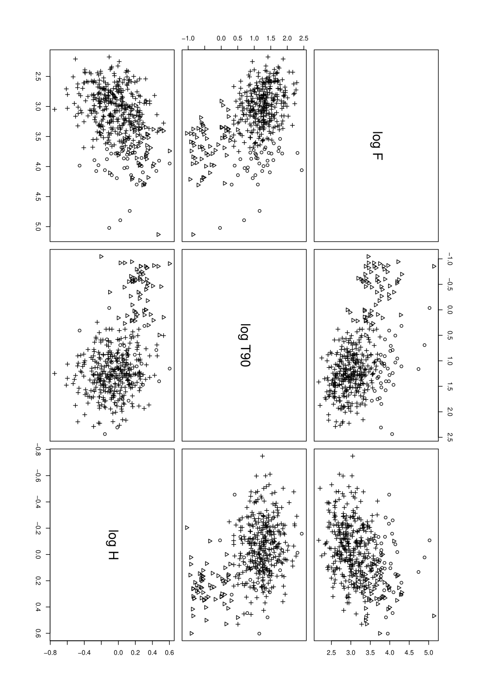
Next we perform model-based clustering on three variables: durations, hardnesses , and peak-count rates . Since the peak rates were measured for all events, the sample here also consists of all 427 bursts (Table 9).
The best fitted model has components (see Fig. 9) with equal volumes, equal shapes and equal correlation coefficients between all clusters (EEE model). This best model has a value of . The EEE model with two components gives and for four components . Markedly high values of BIC are also obtained for the EEI, VEI, and VVI models with components, , , and , respectively.
The difference in BIC between the EEE model with three components and the EEE models with two or four components is . The other models with other number of components (except above-mentioned EEI, VEI, and VVI models with three components) gives BIC value lower by at least 10. This provides a strong evidence in the favor of EEE model with components. The group structure of this model with three components is shown in Fig. 10.
The intermediate-duration bursts showed in Fig. 1 are assigned to the short/hard group by this test. A new result here is that the group of long bursts is separated into high- and low-peak flux clusters.
IV.3.4 Model-based clustering - 4 variables
Spectral lags of BATSE GRBs, i.e. the time delay between low and high energy photons from short and long groups have been found to differ. For short bursts, an average lag is times shorter than for long bursts, and the lag distribution is close to symmetric about zero - unlike long bursts [47, 48, 49]. This result gave us an idea to incorporate the spectral lags as well.
In this part we apply the model-based clustering on GRB peak-count rates , durations, hardness ratios , and as a new addition to the variables, on normalized lags . Since the RHESSI spectral lags were calculated only for 142 bursts (Table 9), our sample is truncated.
The best fitted model has components and is unconstrained, i.e. it has variable volumes, variable shapes and variable correlation coefficients (VVV). The best BIC value for this model is . However, the VVV model with components gives similar value of . The other models gives BIC value lower by at least 10. This strongly supports the VVV model with components. There is no need to introduce VVV model with three components that has more free parameters. The two components are separated accordingly to the values of normalized lags into zero- and non-zero-lag events.
IV.3.5 Summary of model-based clustering
The model-based clustering of two-parameter data ( and ) gives a strong evidence in favor of EVI model with two components. The analysis of three-parameter data (, and ) shows that the best fitted model is EEE with three components. Surprisingly a new result is obtained here; the group of long bursts is separated into high- and low-peak flux clusters. The analysis of four-parameter data (, , and ) supports the VVV model with two components only. The separation into the two components here is accordingly to the values of normalized lags into zero- and non-zero-lag events.
| Model | Evidence | |||||||
|---|---|---|---|---|---|---|---|---|
| k=1 | k=2 | k=3 | k=4 | |||||
| 2 par. | EVI | 2 | -681.5 | very strong | ||||
| 3 par. | EEE | 3 | -1156.6 | very strong | ||||
| 4 par. | VVV | 2 | -1768.4 | very strong |
Note. — The results for model-based clustering applied on 2, 3, and 4 parameters is presented. The values of BIC for the best fitted models with components are listed, as well as the differences to the models with other number of components.
IV.3.6 K-means clustering
One of the non-parametric clustering methods is K-means [38]. Before we use our data for this method we scale them, i.e. we subtract the mean value and then divide them by the standard deviation. The reason for this procedure is that the clustering algorithm is sensitive to the distance scale of the variables. For more details about the application of the K-means method in a similar analysis of GRB data, see, e.g. Chattopadhyay et al. [12] or Veres et al. [68]. For this clustering method we use kmeans package implemented in the R software.
To use the K-means method, one must set the number of clusters beforehand. Then the corresponding number of centers is found by minimizing the sum of squared distances from each burst to the center of the group to which they belong. There is no precise way to determine the best number of clusters with this method. However, it has been suggested that if one plots the within-group sum of squares (WSS) as a function of the number of clusters, then an “elbow” will indicate the best number [23]. This method do not provide any probability indicating the significance or insignificance for the given best number of clusters.
The calculated WSS as a function of the number of groups for our data samples using 2 (, ), 3 (, , ), and 4 (, , , ) variables are rather smooth and do not demonstrate any remarkable and sharp “elbows” and thus do not bring useful information on the GRB classification.
IV.4 Discussion of the results
The K-S tests applied on peak-count rates show that the distributions are different over all three groups. The K-S significance level for the short-long pair is %, for the intermediate-long pair it is 10-5 %, and for the intermediate-short one it is 0.9 %. The short and long GRBs have clearly different distributions of peak rates. Also the intermediate and long GRBs have clearly different distributions of peak rates. The intermediate-short pair also exhibits different distributions (K-S probability %), however less markedly than the other pairs of groups do. These results are confirmed by MC simulations.
The A-D tests applied on distributions of spectral lags unveil that the A-D probability for the short-long pair is %, for the intermediate-long pair the A-D probability is 4.2 %, and for the intermediate-short one it is 16.8 %. The short and long GRBs have clearly different distributions of spectral lags. The intermediate and long GRBs have A-D probability %, however in this case the difference is not strong. The intermediate-short pair does not exhibit different distributions. The difference in the spectral lag distributions of the short-long pair of GRB groups is confirmed by MC simulations. In case of intermediate-short and intermediate-long pairs the MC simulations reveal the same tendency as the A-D tests applied directly on the measured values, i.e. the intermediate-short pair has more similar distributions of spectral lags than the intermediate-long pair has. However, MC simulations gives A-D probability higher than 5 % more often then expected. A possible reason is commented in Sec. III.4.
The A-D tests applied on distributions of normalized lags show that these distributions cannot be claimed as different. The A-D probability for the short-long pair is 6.0 %, for the intermediate-long pair it is 45.0 %, and for the intermediate-short one it is 54.2 %. Here one can see the same tendency as in the case of A-D tests applied on spectral lags, i.e. the short-long pair has the least similar distributions of lags, the intermediate-long couple stays in the middle, and the intermediate-short pair has the most similar distributions. This tendency appears also in the MC simulations, however the absolute frequency of the cases when A-D probability exceeds 5 % level happens more often then expected. The reason could be the same as in the case of MC simulations applied on absolute values of spectral lags.
The model-based clustering of two-parameter data ( and ) gives a strong evidence in favor of a model with two components only. The two components are short/hard and long/soft groups. The intermediate-duration bursts showed in Fig. 1 are assigned to the short/hard group by this test. The analysis of three-parameter data (, and ) shows that the best fitted model has three components. Surprising point here is that this method separates the group of long bursts into high- and low-peak flux clusters. The analysis of four-parameter data (, , and ) supports a model with two components which are separated accordingly to the values of normalized lags into zero- and non-zero-lag events.
Surveying the A-D and K-S tests of the RHESSI data, it should be raised that the difference between the short and long bursts was again strongly confirmed. This follows from the different distributions of the spectral lags and by the different distributions of the peak-count rates, both results were confirmed by the MC method. This is already an expectable result, but - usefully - this result came from a new observational database.
According to Fig. 1 the intermediate-short pair of groups have similar hardness ratios. Also according to the results of the A-D test of the spectral lags, the distributions of lags are not different for the intermediate-short pair. However, the intermediate-duration and short-duration bursts are not completely same because their peak-count rate distributions differ. On the other hand, the intermediate-long pair of groups differs in hardness ratios, spec. lags, and peak-count rates. Therefore, in our opinion, it is possible that the intermediate group detected by RHESSI in Sec. II and by [55] may be a longer tail of standard short/hard bursts. This can be supported also by the fact that model-based clustering method applied on hardness ratios and durations unveil only two clusters as the best solution; classical short/hard and long/soft groups, the intermediate-duration bursts are assigned to the short group.
The RHESSI intermediate and long groups seem to be different phenomena. This difference is supported by the distribution of the peak-count rates and spectral lags. The results show that the intermediate group is also “intermediate” with regard to its lags. The intermediate group detected by Swift was found to be related to XRFs [68], and those may in turn belong to the standard long GRBs [33]. In the case of RHESSI, the longer and softer GRBs are more difficult to be detected, because RHESSI’s sensitivity declines rapidly below keV and the weak and soft GRBs are not easily observable [55]. On the other hand, Swift is less sensitive in the photon-energy range keV. But softer GRBs are readily detectable with this instrument. Hence, in our opinion, an instrumental effect may be responsible for that the two satellites (Swift and RHESSI) detected different intermediate groups. This means that - from the statistical point of view - different groups can be found if one looks at different databases.
There are bursts observed with properties similar to the short bursts (hardness, lag) except their durations exceed 2 s. For example, beyond Gehrels et al. [20] and Kann et al. [31] mentioned already in Introduction, Norris & Bonnell [49] claims that “short bursts with extended emission (SGRBEE) can have s”. Furthermore, also others [10] propose the astrophysical fragmentation of the short GRB group.
Concerning SGRBEE, we inspected the light-curves of all 18 RHESSI intermediate bursts, but we found no softer extended emission coming after the main hard spike as is typical for this kind of bursts. Figure 3 of Perley et al. [52] shows that the average duration of the initial spike of an SGRBEE lies between the average durations of short and long bursts. If RHESSI detects only the hard initial spike, and the softer extended emission is lost in the noise, then the detected intermediate group might be polluted by these objects. Therefore, we also checked the light-curves of the RHESSI intermediate bursts as observed by Konus-Wind [3], because it also has a good sensitivity below 50 keV (its range is keV). It has an overlap with the following RHESSI intermediate bursts: GRB 020819A, GRB 030410, GRB 040329, GRB 050530, GRB 070802, GRB 070824, GRB 080408. However, no extended emission was observed for these seven bursts by Konus-Wind. This observation indicates the RHESSI intermediate GRBs should not be dominantly polluted by SGRBEEs.
Furthermore, there are also additional indications that GRBs which do not belong to the long+XRF pair category, may originate from a broad range of astrophysical phenomena. For example, Mukherjee et al. [42] found four subclasses in the BATSE database from the year 1998, but the fourth group was populated by a single GRB. From the statistical point of view, such an object is an outlier of uncertain origin. Likewise, similar situations exist concerning the objects GRB 060614 [20] and GRB 110328A [13]. Any study of such a single unusual object is beyond the scope of this article providing only statistical analyses.
V Conclusions
The main results of this study can be summarized as follows:
- •
Maximum Likelihood test in the duration-hardness plane of 427 RHESSI GRBs, taken from Řípa et al. [55] but now with six events corrected for decimation, again exhibits statistically significant third, in duration intermediate, group. This completes the work Řípa et al. [55] using the durations and hardnesses only.
- •
The spectral lags and peak-count rates have been calculated for GRBs observed by the RHESSI satellite for the first time. The spectral lags were obtained for 142 objects, and the peak-counts for all 427 GRBs. Hence, we constructed a new observational database for this satellite. Then the three GRB subgroups were analyzed statistically with respect to these new spectral lags and peak-count rates.
- •
The difference between short and long groups has been confirmed. Usefully this result came from a new observational database.
- •
Kolmogorov-Smirnov and Anderson-Darling tests applied on spectral lags and peak-count rates indicate that the intermediate group in the RHESSI database might be a longer tail of the short group or at least has some common properties with this short group. Contrary to this, the intermediate and the long groups are different.
- •
The group of RHESSI intermediate-duration GRBs is not dominantly populated by SGRBEEs.
- •
The intermediate-duration bursts found in the RHESSI and Swift databases seem to be represented by different phenomena.
| GRBaaRHESSI GRB number. | GroupbbThe assignment to the GRB group: 1 - short,
2 - intermediate, 3 - long. |
(ms)ccSpectral lags were calculated from the difference of the count light-curves at the energy intervals keV and keV. The errors compose of the 95 % CL statistical uncertainty and the light-curve’s time resolution. | (s-1)ddPeak-count rates derived in the band keV. | (s-1)eeOne sigma statistical uncertainties of the peak-count rates. |
|---|---|---|---|---|
| 020214 | 3 | 42.4 | 8885.9 | 221.3 |
| 020218 | 3 | 607.0 | 3630.7 | 92.9 |
| 020302 | 3 | 632.6 | 62.7 | |
| 020306 | 1 | 1.2 | 9003.0 | 867.4 |
| 020311 | 3 | 641.9 | 1571.9 | 119.7 |
| 020313 | 3 | 891.2 | 89.3 | |
| 020315 | 3 | 504.1 | 91.6 | |
| 020331 | 3 | 307.2 | 71.8 | |
| 020407 | 3 | 775.9 | 72.4 | |
| 020409 | 3 | 268.6 | 56.0 | |
| 020413 | 3 | 1153.5 | 130.8 | |
| 020417 | 3 | 846.8 | 77.1 | |
| 020418 | 3 | 108.6 | 5618.8 | 289.6 |
| 020426 | 1 | 3873.5 | 436.2 | |
| 020430 | 3 | 1209.8 | 100.9 | |
| 020509 | 3 | 2785.5 | 310.0 | |
| 020524 | 3 | 958.1 | 116.7 | |
| 020525A | 3 | 452.4 | 975.4 | 159.5 |
| 020525B | 1 | 3265.2 | 526.6 | |
| 020527 | 2 | 1467.1 | 278.8 | |
| 020602 | 3 | 2643.6 | 503.4 | |
| 020603 | 3 | 6473.9 | 1042.8 | |
| 020604 | 3 | 1187.1 | 98.9 | |
| 020620 | 3 | 1816.7 | 260.3 | |
| 020623 | 3 | 962.8 | 169.9 | |
| 020630 | 3 | 997.8 | 94.1 | |
| 020702 | 3 | 803.6 | 98.2 | |
| 020708 | 3 | 383.9 | 45.8 | |
| 020712 | 3 | 724.5 | 115.8 | |
| 020715A | 1 | 2449.4 | 397.6 | |
| 020715B | 3 | 135.7 | 10359.6 | 247.5 |
| 020725 | 3 | 3985.2 | 469.3 | |
| 020801 | 3 | 1740.8 | 384.4 | |
| 020819A | 2 | 170.6 | 2235.2 | 353.0 |
| 020819B | 3 | 1014.4 | 96.3 | |
| 020828 | 1 | 6.3 | 5356.8 | 862.4 |
| 020910 | 3 | 1792.6 | 215.3 | |
| 020914 | 3 | 1284.7 | 268.7 | |
| 020926 | 3 | 618.9 | 63.2 | |
| 021008A | 3 | 12.5 | 54724.6 | 1415.5 |
| 021008B | 3 | 556.5 | 108.6 | |
| 021011 | 3 | 771.1 | 157.9 | |
| 021016 | 3 | 647.3 | 98.0 | |
| 021020 | 3 | 2275.6 | 125.7 | |
| 021023 | 3 | 1787.9 | 270.7 | |
| 021025 | 3 | 645.3 | 91.9 | |
| 021102 | 3 | 1796.7 | 112.4 | |
| 021105 | 3 | 818.0 | 163.6 | |
| 021108 | 3 | 1072.2 | 87.1 | |
| 021109 | 3 | 903.3 | 85.7 | |
| 021113 | 3 | 374.3 | 89.6 | |
| 021115 | 3 | 484.9 | 89.2 | |
| 021119 | 3 | -393.8 | 2129.7 | 277.4 |
| 021125 | 3 | 1434.5 | 174.4 | |
| 021201 | 1 | 10.5 | 9868.9 | 1044.7 |
| 021205 | 3 | 579.2 | 39.4 | |
| 021206 | 3 | 8.9 | 78241.5 | 3719.6 |
| 021211 | 3 | 1649.6 | 409.6 | |
| 021214 | 3 | 279.9 | 44.6 | |
| 021223 | 3 | 1169.7 | 338.0 | |
| 021226 | 1 | 16.3 | 5997.7 | 403.9 |
| 030102 | 3 | 1125.4 | 99.1 | |
| 030103 | 3 | 245.3 | 61.2 | |
| 030105 | 2 | 6.7 | 4873.4 | 465.0 |
| 030110 | 1 | 2791.2 | 714.4 | |
| 030115A | 3 | 328.0 | 1433.8 | 145.1 |
| 030115B | 3 | 970.4 | 214.2 | |
| 030127 | 3 | 779.9 | 133.1 | |
| 030204 | 3 | 196.0 | 2093.2 | 68.3 |
| 030206 | 1 | -6.6 | 3982.8 | 553.3 |
| 030212 | 3 | 726.2 | 175.5 | |
| 030214 | 3 | 2164.6 | 168.9 | |
| 030216 | 3 | 530.3 | 93.7 | |
| 030217 | 3 | 5531.9 | 548.3 | |
| 030222 | 3 | 772.4 | 89.4 | |
| 030223 | 3 | 1108.2 | 857.3 | 87.0 |
| 030225 | 3 | 1338.1 | 566.8 | 67.7 |
| 030227 | 3 | -1374.2 | 358.0 | 69.8 |
| 030228 | 3 | 1281.8 | 147.4 | |
| 030301 | 3 | 381.6 | 93.5 | |
| 030306 | 3 | 2740.5 | 135.1 | |
| 030307 | 3 | 248.3 | 7542.7 | 302.7 |
| 030320A | 3 | 358.1 | 1782.3 | 198.9 |
| 030320B | 3 | 415.8 | 622.6 | 29.4 |
| 030326 | 3 | 2034.3 | 116.4 | |
| 030328 | 3 | 891.1 | 141.0 | |
| 030329A | 3 | 37.5 | 11876.3 | 219.7 |
| 030329B | 3 | 531.8 | 49.5 | |
| 030331 | 3 | 1148.8 | 221.9 | |
| 030406 | 3 | 240.6 | 6067.2 | 283.3 |
| 030410 | 2 | 23.1 | 2392.8 | 308.2 |
| 030413 | 3 | -257.9 | 1181.4 | 109.1 |
| 030414 | 3 | 1171.0 | 2599.3 | 96.8 |
| 030419 | 3 | 7826.4 | 226.3 | |
| 030421 | 3 | 69.0 | 4489.0 | 525.3 |
| 030422 | 3 | 700.1 | 102.2 | |
| 030428 | 3 | 24.9 | 5294.8 | 190.8 |
| 030501A | 3 | 1961.3 | 146.9 | |
| 030501B | 3 | 404.4 | 96.2 | |
| 030501C | 2 | 3029.0 | 600.2 | |
| 030505A | 3 | 584.9 | 112.9 | |
| 030505B | 3 | -267.8 | 1448.6 | 46.9 |
| 030506 | 3 | 1315.8 | 186.0 | |
| 030518A | 3 | 81.2 | 7982.3 | 640.6 |
| 030518B | 3 | 1867.0 | 248.6 | |
| 030519A | 3 | 1890.9 | 318.7 | |
| 030519B | 3 | 17.0 | 15592.7 | 299.0 |
| 030523 | 1 | 2828.1 | 485.7 | |
| 030528 | 3 | 423.7 | 69.7 | |
| 030601 | 3 | 465.6 | 1051.9 | 98.4 |
| 030614 | 3 | 898.5 | 32.7 | |
| 030626 | 3 | 333.6 | 1434.1 | 78.0 |
| 030703 | 3 | 229.4 | 54.0 | |
| 030706 | 3 | 1021.3 | 101.4 | |
| 030710 | 3 | 1114.7 | 97.7 | |
| 030714 | 3 | 1499.3 | 129.3 | |
| 030716 | 3 | 377.2 | 68.3 | |
| 030721 | 3 | 59.9 | 12474.1 | 679.8 |
| 030725 | 3 | 1014.1 | 93.0 | |
| 030726A | 3 | 57.8 | 2005.1 | 94.7 |
| 030726B | 3 | 400.9 | 51.9 | |
| 030728 | 3 | 655.4 | 127.2 | |
| 030824 | 3 | 509.0 | 86.0 | |
| 030827 | 3 | 18.4 | 3678.2 | 355.2 |
| 030830 | 3 | 1835.5 | 87.4 | |
| 030831 | 3 | 1903.3 | 123.3 | |
| 030919 | 3 | 828.7 | 143.0 | |
| 030921 | 3 | 2414.9 | 127.7 | |
| 030922A | 3 | 1418.7 | 111.6 | |
| 030922B | 3 | 38.7 | 4042.1 | 171.3 |
| 030926 | 1 | 2094.0 | 422.3 | |
| 031005 | 3 | 661.9 | 132.6 | |
| 031019 | 3 | 1260.8 | 160.4 | |
| 031024 | 3 | 218.6 | 3055.6 | 552.4 |
| 031027 | 3 | 128.2 | 4102.5 | 113.9 |
| 031107 | 3 | -121.0 | 1183.0 | 86.4 |
| 031108 | 3 | 88.9 | 5923.9 | 157.4 |
| 031111 | 3 | 57.1 | 13882.4 | 445.7 |
| 031118 | 1 | 4669.8 | 592.7 | |
| 031120 | 3 | 1147.6 | 991.2 | 57.3 |
| 031127 | 3 | 634.4 | 94.5 | |
| 031130 | 3 | 1354.9 | 155.0 | |
| 031214 | 3 | 609.8 | 159.3 | |
| 031218 | 1 | 53.4 | 4732.5 | 1067.7 |
| 031219 | 3 | 334.0 | 3262.1 | 439.7 |
| 031226 | 3 | 640.4 | 72.5 | |
| 031226 | 3 | 612.8 | 86.8 | |
| 040102 | 3 | 1160.1 | 139.1 | |
| 040108 | 3 | 395.7 | 70.3 | |
| 040113 | 3 | 1183.6 | 193.7 | |
| 040115 | 3 | 473.1 | 84.0 | |
| 040125 | 3 | 528.6 | 111.7 | |
| 040205A | 3 | 497.4 | 152.7 | |
| 040205B | 3 | 378.0 | 76.3 | |
| 040207 | 3 | 23.6 | 3375.9 | 115.9 |
| 040211 | 3 | 751.8 | 181.5 | |
| 040215 | 3 | 391.7 | 46.9 | |
| 040220 | 3 | 1041.1 | 1714.0 | 178.9 |
| 040225A | 3 | 576.5 | 104.0 | |
| 040225B | 3 | 642.5 | 90.0 | |
| 040228 | 3 | 19.2 | 11483.8 | 261.6 |
| 040302A | 3 | 712.0 | 98.2 | |
| 040302B | 3 | 101.8 | 13904.2 | 283.4 |
| 040303 | 3 | 403.8 | 86.2 | |
| 040312 | 1 | 2.7 | 7197.9 | 690.1 |
| 040316 | 3 | -161.3 | 4356.0 | 452.4 |
| 040323 | 3 | 650.8 | 174.9 | |
| 040324 | 1 | 2.7 | 16984.5 | 1112.0 |
| 040327 | 3 | 405.8 | 56.2 | |
| 040329 | 2 | 3.6 | 19974.8 | 849.1 |
| 040330 | 3 | 584.5 | 98.3 | |
| 040404 | 3 | 1096.6 | 183.6 | |
| 040413 | 1 | 5163.3 | 594.7 | |
| 040414 | 3 | 992.3 | 59.5 | |
| 040421 | 3 | 98.6 | 7197.3 | 220.2 |
| 040423 | 3 | 663.4 | 111.5 | |
| 040425 | 3 | 155.3 | 7424.3 | 843.8 |
| 040427 | 3 | 674.8 | 112.1 | |
| 040429 | 3 | 582.8 | 85.4 | |
| 040502A | 3 | 3551.8 | 310.5 | |
| 040502B | 3 | 602.9 | 48.9 | |
| 040506 | 3 | 807.0 | 61.2 | |
| 040508 | 3 | 242.0 | 64.4 | |
| 040510 | 3 | 1097.3 | 123.3 | |
| 040513 | 3 | 218.9 | 49.2 | |
| 040526 | 3 | 499.1 | 96.2 | |
| 040528 | 3 | 731.5 | 1827.0 | 119.2 |
| 040531 | 3 | 1024.5 | 75.3 | |
| 040601 | 3 | 401.3 | 93.9 | |
| 040603A | 3 | 726.3 | 138.6 | |
| 040603B | 3 | 161.9 | 26.5 | |
| 040605A | 3 | 800.3 | 224.4 | |
| 040605B | 1 | 26.0 | 8657.1 | 1243.4 |
| 040605C | 3 | 1271.6 | 87.0 | |
| 040611 | 3 | -2267.0 | 740.1 | 87.8 |
| 040619 | 3 | 3308.1 | 480.5 | |
| 040701 | 3 | 135.0 | 1128.0 | 103.9 |
| 040719 | 3 | 1445.1 | 177.0 | |
| 040723 | 3 | 4168.6 | 697.7 | |
| 040731 | 3 | 110.2 | 1803.4 | 91.5 |
| 040803 | 3 | 267.3 | 39.1 | |
| 040810 | 3 | 1654.2 | 109.7 | |
| 040818 | 3 | 33.2 | 2681.5 | 225.6 |
| 040822 | 2 | 2226.7 | 374.5 | |
| 040824 | 3 | 282.2 | 45.8 | |
| 040921 | 1 | 2619.0 | 490.6 | |
| 040925 | 3 | -136.0 | 1263.8 | 167.1 |
| 040926 | 3 | 4.1 | 5855.8 | 207.3 |
| 041003 | 3 | 735.4 | 182.2 | |
| 041006 | 3 | 1307.7 | 254.1 | |
| 041007 | 2 | 101.0 | 3301.3 | 238.6 |
| 041009 | 3 | 1382.6 | 111.5 | |
| 041010 | 1 | 0.7 | 1838.8 | 616.2 |
| 041012 | 3 | 276.6 | 44.5 | |
| 041013A | 3 | 530.3 | 39.7 | |
| 041013B | 1 | 3412.2 | 421.8 | |
| 041015 | 3 | 1630.8 | 189.7 | |
| 041016 | 3 | 509.0 | 78.5 | |
| 041018 | 3 | 6774.4 | 717.6 | 120.4 |
| 041101 | 3 | 1036.3 | 167.5 | |
| 041102 | 3 | 1437.3 | 188.3 | |
| 041107 | 3 | 883.0 | 83.3 | |
| 041116 | 3 | 269.7 | 52.1 | |
| 041117 | 3 | 1165.2 | 106.5 | |
| 041120 | 3 | 1167.1 | 123.6 | |
| 041125 | 3 | -7.8 | 9489.2 | 168.7 |
| 041202 | 3 | 76.3 | 5824.1 | 198.0 |
| 041211A | 3 | 56.3 | 1066.9 | 83.9 |
| 041211B | 3 | 5126.6 | 629.1 | |
| 041211C | 3 | -6.0 | 11832.5 | 315.0 |
| 041213 | 1 | 6872.1 | 669.2 | |
| 041218 | 3 | 364.9 | 54.7 | |
| 041219 | 3 | 560.3 | 76.9 | |
| 041223 | 3 | -1.6 | 1567.8 | 91.6 |
| 041224 | 3 | 285.4 | 73.2 | |
| 041231 | 2 | 21.6 | 2211.1 | 206.3 |
| 050124 | 3 | 815.2 | 162.3 | |
| 050126 | 3 | 1477.0 | 79.6 | |
| 050203 | 3 | 2870.6 | 234.3 | |
| 050213 | 3 | 44.2 | 2174.0 | 101.5 |
| 050214 | 3 | 390.4 | 60.3 | |
| 050216 | 1 | 6.0 | 4614.1 | 686.4 |
| 050219 | 3 | 410.8 | 4760.8 | 259.7 |
| 050311 | 3 | 465.1 | 88.4 | |
| 050312 | 1 | 4.4 | 4439.8 | 419.4 |
| 050314 | 3 | 2101.0 | 151.0 | |
| 050320 | 3 | 838.7 | 114.5 | |
| 050321 | 3 | 880.5 | 128.4 | |
| 050326 | 3 | 3501.9 | 403.9 | |
| 050328 | 1 | -43.5 | 12706.3 | 1069.6 |
| 050404 | 3 | 29.1 | 6336.6 | 215.9 |
| 050409 | 2 | -1.7 | 18969.8 | 1936.7 |
| 050411 | 3 | 813.9 | 125.9 | |
| 050412 | 3 | 1455.7 | 140.8 | |
| 050429 | 3 | 2018.6 | 145.8 | |
| 050430 | 3 | 986.8 | 139.4 | |
| 050501 | 3 | 1697.9 | 308.8 | |
| 050502 | 2 | 1132.2 | 235.6 | |
| 050509 | 3 | -63.6 | 2282.4 | 145.7 |
| 050516 | 3 | 259.7 | 71.5 | |
| 050525A | 3 | 4853.5 | 259.6 | |
| 050525B | 3 | 8.5 | 7311.6 | 214.3 |
| 050528 | 3 | 421.3 | 48.7 | |
| 050530 | 3 | 1963.1 | 273.3 | |
| 050531 | 3 | 56.6 | 6082.8 | 197.2 |
| 050614 | 3 | 377.5 | 58.6 | |
| 050701 | 3 | 1173.5 | 166.1 | |
| 050702 | 2 | 951.9 | 187.8 | |
| 050703 | 3 | 2734.2 | 305.4 | |
| 050706 | 3 | 1620.7 | 168.6 | |
| 050713A | 3 | -233.3 | 1450.6 | 244.4 |
| 050713B | 3 | 431.1 | 69.1 | |
| 050715 | 3 | 2053.4 | 198.9 | |
| 050717 | 3 | 110.3 | 2456.3 | 143.1 |
| 050726 | 3 | 810.5 | 1480.4 | 90.7 |
| 050729 | 3 | 873.7 | 177.5 | |
| 050802 | 3 | 498.5 | 97.6 | |
| 050805 | 2 | -6.2 | 3355.3 | 334.6 |
| 050809 | 3 | 4598.3 | 699.3 | |
| 050813 | 3 | 810.7 | 110.4 | |
| 050814 | 1 | 5499.5 | 1658.3 | |
| 050817 | 3 | 895.5 | 118.2 | |
| 050820 | 3 | 681.3 | 101.9 | |
| 050824 | 1 | 1.2 | 7474.8 | 930.5 |
| 050825 | 2 | -82.6 | 4307.4 | 585.3 |
| 050902 | 3 | 631.9 | 149.5 | |
| 050923 | 3 | 1872.2 | 395.3 | |
| 051009 | 3 | 475.8 | 66.9 | |
| 051012 | 3 | 462.5 | 3780.0 | 331.8 |
| 051021 | 3 | -97.8 | 2117.7 | 221.7 |
| 051031 | 3 | 678.7 | 45.4 | |
| 051101 | 3 | 921.2 | 258.0 | |
| 051103 | 1 | 0.6 | 135199.6 | 10873.8 |
| 051109 | 3 | 882.0 | 92.0 | |
| 051111 | 3 | 516.1 | 102.1 | |
| 051117 | 3 | -224.8 | 942.4 | 133.9 |
| 051119 | 3 | 743.4 | 133.7 | |
| 051124A | 3 | 1234.2 | 194.2 | |
| 051124B | 3 | 2715.0 | 152.8 | |
| 051201A | 3 | 211.7 | 37.0 | |
| 051201B | 3 | 1000.9 | 170.4 | |
| 051207 | 3 | 2440.2 | 121.2 | |
| 051211 | 3 | 592.3 | 1573.5 | 69.6 |
| 051217 | 3 | 458.7 | 81.7 | |
| 051220A | 3 | 39.0 | 19918.0 | 658.7 |
| 051220B | 3 | 321.2 | 73.1 | |
| 051221 | 1 | 0.0 | 15280.2 | 1298.8 |
| 051222 | 3 | 334.4 | 78.5 | |
| 060101 | 3 | 599.3 | 1647.1 | 94.2 |
| 060110 | 3 | 445.6 | 107.8 | |
| 060111 | 3 | -2346.6 | 1079.4 | 46.7 |
| 060117 | 3 | 1300.6 | 113.7 | |
| 060121A | 3 | 2980.4 | 277.6 | |
| 060121B | 3 | 343.0 | 46.7 | |
| 060123 | 3 | 18.4 | 3965.2 | 184.2 |
| 060124 | 3 | 713.2 | 76.3 | |
| 060130 | 3 | 2285.1 | 376.4 | |
| 060203 | 1 | -23.5 | 6089.8 | 831.6 |
| 060217 | 3 | 2432.4 | 416.0 | |
| 060224 | 3 | -944.0 | 851.0 | 109.2 |
| 060228 | 3 | -702.0 | 717.4 | 89.8 |
| 060303 | 1 | 21.2 | 9343.4 | 999.5 |
| 060306 | 3 | 50.3 | 105153.0 | 3272.9 |
| 060309 | 3 | 355.6 | 62.1 | |
| 060312A | 1 | 1526.6 | 337.6 | |
| 060312B | 3 | 299.2 | 71.4 | |
| 060313 | 3 | 602.2 | 103.3 | |
| 060323 | 3 | -186.2 | 3754.8 | 169.1 |
| 060325 | 3 | 189.3 | 6080.4 | 638.4 |
| 060401 | 3 | 110.2 | 2527.5 | 208.8 |
| 060408 | 3 | 449.7 | 85.1 | |
| 060415 | 3 | 315.7 | 78.6 | |
| 060418 | 3 | 694.3 | 74.4 | |
| 060421A | 3 | 789.4 | 78.5 | |
| 060421B | 3 | 312.3 | 2812.8 | 106.2 |
| 060425 | 1 | 5.3 | 2367.7 | 521.1 |
| 060428 | 3 | 274.9 | 60.2 | |
| 060429 | 1 | 3.2 | 20278.7 | 2240.6 |
| 060505 | 3 | 277.1 | 1384.9 | 256.7 |
| 060528 | 3 | 2441.1 | 656.8 | 77.5 |
| 060530 | 3 | 889.0 | 143.9 | |
| 060610 | 1 | 10.0 | 9569.6 | 748.7 |
| 060614 | 3 | 498.7 | 40.7 | |
| 060622 | 3 | -1510.2 | 1038.4 | 71.5 |
| 060624 | 3 | 9648.0 | 610.3 | |
| 060625 | 3 | 1179.5 | 122.8 | |
| 060630 | 3 | 1377.2 | 83.7 | |
| 060708 | 1 | -5.6 | 16293.3 | 1641.8 |
| 060729 | 3 | 588.4 | 100.8 | |
| 060805 | 3 | 18.3 | 10612.2 | 474.3 |
| 060811 | 3 | 1742.2 | 103.9 | |
| 060819 | 3 | 949.2 | 159.3 | |
| 060823 | 2 | 811.4 | 167.0 | |
| 060919 | 3 | 368.6 | 61.5 | |
| 060920 | 3 | 22.4 | 4809.8 | 181.2 |
| 060925 | 3 | 1840.6 | 114.1 | |
| 060928 | 3 | 144.7 | 5934.5 | 281.3 |
| 061005 | 3 | 2187.7 | 239.8 | |
| 061006A | 1 | 9.4 | 6404.0 | 940.7 |
| 061006B | 2 | 2359.0 | 286.1 | |
| 061007 | 3 | 66.2 | 3465.1 | 305.1 |
| 061012 | 3 | 1474.0 | 171.6 | |
| 061013 | 3 | 776.2 | 102.5 | |
| 061014 | 1 | 2308.8 | 291.6 | |
| 061022 | 3 | 392.3 | 77.3 | |
| 061031 | 3 | 1112.8 | 238.5 | |
| 061101 | 3 | 631.7 | 88.3 | |
| 061108 | 3 | 2267.8 | 219.2 | |
| 061113 | 3 | 36.4 | 3665.0 | 233.6 |
| 061117 | 3 | 251.6 | 56.0 | |
| 061121 | 3 | -57.8 | 3131.4 | 176.9 |
| 061123 | 3 | 1360.8 | 172.8 | |
| 061126 | 3 | 194.3 | 2897.4 | 120.5 |
| 061128 | 1 | -3.0 | 15183.0 | 1310.9 |
| 061205 | 3 | 427.5 | 83.8 | |
| 061212 | 3 | 13.0 | 9820.5 | 440.1 |
| 061222 | 3 | 1367.9 | 263.2 | |
| 061229 | 3 | 680.4 | 68.7 | |
| 061230 | 3 | 641.3 | 133.8 | |
| 070113 | 1 | 1986.8 | 377.5 | |
| 070116 | 3 | 736.2 | 111.8 | |
| 070120 | 3 | 395.8 | 70.0 | |
| 070121 | 3 | 178.8 | 49.4 | |
| 070125 | 3 | -9.6 | 4841.5 | 149.0 |
| 070214 | 3 | 425.7 | 98.3 | |
| 070220 | 3 | 972.7 | 103.0 | |
| 070221 | 3 | 511.0 | 103.0 | |
| 070307 | 3 | 502.2 | 56.2 | |
| 070402 | 3 | 829.0 | 113.1 | |
| 070420 | 3 | 509.7 | 87.5 | |
| 070508 | 3 | 1627.4 | 168.9 | |
| 070516 | 1 | 28.9 | 2376.6 | 268.6 |
| 070531 | 3 | 149.7 | 34.0 | |
| 070614 | 1 | 2.4 | 2874.7 | 275.5 |
| 070622 | 3 | 39.9 | 3397.0 | 207.5 |
| 070626 | 3 | 2058.8 | 111.6 | |
| 070710 | 3 | 379.1 | 66.7 | |
| 070717 | 3 | 347.5 | 59.0 | |
| 070722 | 3 | 321.7 | 77.4 | |
| 070724 | 3 | 259.1 | 37.5 | |
| 070802 | 3 | 15.8 | 2426.5 | 234.0 |
| 070817 | 3 | 541.2 | 55.5 | |
| 070819 | 3 | 915.7 | 75.6 | |
| 070821 | 3 | 663.0 | 1956.7 | 77.2 |
| 070824 | 2 | -5.9 | 3276.6 | 284.3 |
| 070825 | 3 | 875.1 | 1335.1 | 94.6 |
| 070917 | 3 | 347.2 | 65.7 | |
| 071013 | 3 | 963.7 | 211.9 | |
| 071014 | 3 | 1094.5 | 155.0 | |
| 071030 | 3 | 570.0 | 82.8 | |
| 071104 | 3 | 747.0 | 98.2 | |
| 071204 | 1 | 2901.5 | 297.5 | |
| 071217 | 3 | 814.3 | 143.8 | |
| 080114 | 3 | 285.7 | 2321.1 | 144.3 |
| 080202 | 3 | 462.1 | 75.7 | |
| 080204 | 3 | 60.5 | 1368.6 | 180.0 |
| 080211 | 3 | 1139.6 | 1349.4 | 143.3 |
| 080218 | 3 | 404.1 | 85.2 | |
| 080224 | 3 | 1795.1 | 186.7 | |
| 080318 | 3 | 385.3 | 90.3 | |
| 080319 | 3 | 157.9 | 885.8 | 111.1 |
| 080320 | 3 | 34.0 | 1722.6 | 110.4 |
| 080328 | 3 | 886.7 | 47.1 | |
| 080330 | 3 | 26.3 | 1685.0 | 98.1 |
| 080408 | 2 | 73.3 | 2546.1 | 353.7 |
| 080413 | 3 | 544.1 | 141.2 | |
| 080425 | 3 | 674.6 | 120.5 |
Appendix A Uncertainties of Decimated Data
This part describes the one sigma uncertainties of the bin counts for the decimated RHESSI data [14, 63].
A.1 Full decimation
Calculation of one sigma uncertainty for the bin counts of fully decimated data and then corrected for this decimation is the following. For corrected bin counts it holds:
| (A1) |
where is the decimation factor (weight), usually equal to 4 or 6 for the RHESSI data, and is the number of counts in a bin of the decimated signal. If we assume that counts in a bin follow Poisson statistics then:
| (A2) |
where is the dispersion of the .
A.2 Partial decimation
Now consider the situation in which counts in a bin are only partially decimated, i.e. they consists of the non-decimated and the decimated signal . This situation may happen when we sum counts over the energy band , , and only the counts below the energy are decimated. Then the corrected signal is equal to:
| (A3) |
where is again the decimation factor, and is corrected part of the signal that was decimated. One sigma uncertainty is then equal to:
| (A4) |
where is the dispersion of the non-decimated part of the bin counts and is the dispersion of the decimated part of the bin counts.
References
- [1] Anderson, T. W., & Darling, D. A. 1952, The Annals of Mathematical Statistics, 23, 193
- [2] Darling, D. A. 1957, The Annals of Mathematical Statistics, 28, 823
- [3] Aptekar, R. L., et al. 1995, Space Science Reviews, 71, 265
- [4] Aptekar, R. L., et al. 1998, in AIP Conf. Proc., Fourth Huntsville Gamma-Ray Burst Symposium, eds. C. A. Meegan, T. M. Koshut, & R. D. Preece, 428, 10
- [5] Bagoly, Z., et al. 2006, A&A, 453, 797
- [6] Balastegui, A., Ruiz-Lapuente, P., & Canal, R. 2001, MNRAS, 328, 283
- [7] Balázs, L. G., Mészáros, A., & Horváth, I. 1998, A&A, 339, 1
- [8] Balázs, L. G., Mészáros, A., Horváth, I., & Vavrek, R. 1999, A&AS, 138, 417
- [9] Balázs, L. G., Bagoly, Z., Horváth, I., Mészáros, A., & Mészáros, P. 2003, A&A, 401, 129
- [10] de Barros, G., Amati, L., Bernardini, M. G., Bianco, C. L., Caito, L., Izzo, L., Patricelli, B., & Ruffini, R. 2011, A&A, 529, A130
- [11] Bellm, E. C., Bandstra, M. E., Boggs, S. E., Hajdas, W., Hurley, K., Smith, D. M., & Wigger, C. 2008, in AIP Conf. Proc., GAMMA-RAY BURSTS 2007: Proceedings of the Santa Fe Conference, eds. M. Galassi, D. Palmer, & E. Fenimore, 1000, 154
- [12] Chattopadhyay, T., Misra, R., Chattopadhyay, A. K., & Naskar, M. 2007, ApJ, 667, 1017
- [13] Cummings, J. R. 2011, GCN, 11823
- [14] Curtis, D. W., Berg, P., Gordon, D., Harvey, P. R., Smith, D. M., & Zehnder, A. 2002, Sol. Phys., 210, 115
- [15] Everitt, B. S., Landau, S., Leese, M., & Stahl, D. 2011, Cluster Analysis, 5th edition, Wiley Series in Probability and Statistics, Wiley
- [16] Foley, S., McGlynn, S., Hanlon, L., McBreen, S., & McBreen, B. 2008, A&A, 484, 143
- [17] Foley, S., McGlynn, S., Hanlon, L., McBreen, S., Martin-Carrillo, A., McBreen, B., Topinka, M., & Meehan, S. 2009, Baltic Astronomy, Proceedings of the INTEGRAL/BART Workshop 2009, eds. R. Hudec, J. Řípa, M. Kocka, & R. Havlíková, 18, 279
- [18] Fox, D. B., et al. 2005, Nature, 437, 845
- [19] Fraley, C., & Raftery, A. E. 2000, Journal of the American Statistical Association, 97, 611
- [20] Gehrels, N., et al. 2006, Nature, 444, 1044
- [21] Gendre, B., Galli, A., & Piro, L. 2007, A&A, 465, L13
- [22] Hakkila, J., Haglin, D. J., Pendleton, G. N., Mallozzi, R. S., Meegan, C. A., & Roiger, R. J. 2000, ApJ, 538, 165
- [23] Hartigan, J. A. 1975, Clustering Algorithms, Vol. 13, 351, New York, Wiley
- [24] Horváth, I. 1998, ApJ, 508, 757
- [25] Horváth, I. 2002, A&A, 392, 791
- [26] Horváth, I. 2009, Ap&SS, 323, 83
- [27] Horváth, I., Balázs, L. G., Bagoly, Z., Ryde, F., & Mészáros, A. 2006, A&A, 447, 23
- [28] Horváth, I., Balázs, L. G., Bagoly, Z., & Veres, P. 2008, A&A, 489, L1
- [29] Horváth, I., Bagoly, Z., Balázs, L. G., de Ugarte Postigo, A., Veres, P. & Mészáros, A. 2010, ApJ, 713, 552
- [30] Huja, D., Mészáros, A., & Řípa, J. 2009, A&A, 504, 67
- [31] Kann, D. A., et al. 2011, ApJ, 734, 96
- [32] Kass, R. E., & Raftery, A. E. 1995, Journal of the American Statistical Association, 90, 773
- [33] Kippen, R. M., Woods, P. M., Heise, J., in’t Zand, J. J. M., Briggs, M. S., & Preece, R. D. 2003, AIP Conf. Proc., Gamma-Ray Burst and Afterglow Astronomy 2001: A Workshop Celebrating the First Year of the HETE Mission, eds. G. R. Ricker & R. K. Vanderspek, 662, 244
- [34] Kolmogorov, A. 1933, Giornale dell’Istituto Italiano degli Attuari, 4, 83
- [35] Kouveliotou, C., Meegan, C. A., Fishman, G. J., Bhat, N. P., Briggs, M. S., Koshut, T. M., Paciesas, W. S., & Pendleton, G. N. 1993, ApJ, 413, L101
- [36] Lin, R. P., et al. 2002, Sol. Phys., 210, 3
- [37] Litvin, V. F., Matveev, S. A., Mamedov, S. V., & Orlov, V. V. 2001, Astronomy Letters, 27, 416
- [38] MacQueen, J. 1967, Fifth Berkeley Symp. Math. Statist. Prob., 1, 281
- [39] Mazets, E. P., et al. 1981, Ap&SS, 80, 3
- [40] McLachlan, G. & Peel, D. 2000, Finite Mixture Models, Wiley Series in Probability and Statistics, Wiley-Interscience
- [41] Mészáros, A., Bagoly, Z., & Vavrek, R. 2000, A&A, 354, 1
- [42] Mukherjee, S., Feigelson, E. D., Jogesh Babu, G., Murtagh, F., Fraley, C., & Raftery, A. 1998, ApJ, 508, 314
- [43] Mészáros, A., & Štoček, J. 2003, A&A, 403, 443
- [44] Nakar, E. 2007, Phys. Rep. 442, 166
- [45] Norris, J. P., Cline, T. L., Desai, U. D., & Teegarden, B. J. 1984, Nature, 308, 434
- [46] Norris, J. P., Marani, G. F., & Bonnell, J. T. 2000, ApJ, 534, 248
- [47] Norris, J. P., Scargle, J. D., & Bonnell, J. T. 2001, Gamma-ray Bursts in the Afterglow Era: Proceedings of the International Workshop Held in Roma, eds. E. Costa, F. Frontera, J. Hjorth, 40
- [48] Norris, J. P. 2002, ApJ, 579, 386
- [49] Norris, J. P., & Bonnell, J. T. 2006, ApJ, 643, 266
- [50] O’Shaughnessy, R., Belczynski, K., & Kalogera, V. 2008, ApJ, 675, 566
- [51] Pendleton, G. N., et al. 1997, ApJ, 489, 175
- [52] Perley, D. A., et al. 2009, ApJ, 696, 1871
- [53] R Development Core Team 2011, R: A Language and Environment for Statistical Computing, Vienna, Austria
- [54] Rajaniemi, H. J., & Mähönen, P. 2002, ApJ, 566, 202
- [55] Řípa, J., Mészáros, A., Wigger, C., Huja, D., Hudec, R., & Hajdas, W. 2009, A&A, 498, 399
- [56] Řípa, J., Veres, P. & Wigger, C. 2010, in Proc. of the Venice (Italy) Conference, The Shocking Universe, eds. G. Chincarini et al., Soc. Ital. Fisica, Bologna, 102, 569
- [57] Sakamoto, T., et al. 2008, ApJS, 175, 179
- [58] Sakamoto, T., & Gehrels, N. 2009, in AIP Proc., Gamma-Ray Burst: Sixth Huntsville Symp., eds. C. Meegan, C. Kouveliotou, N. Gehrels, 1133, 112
- [59] Scholz, F. W., & Stephens, M. A., Journal of the American Statistical Association, 82, 918
- [60] Schwarz, G. 1978, The Annals of Statistics, 6, 461
- [61] Soderberg, A. M., et al. 2006, Nature, 442, 1014
- [62] Smirnov, N. V. 1948, Annals of Mathematical Statistics, 19, 279
- [63] Smith, D. M., et al. 2002, Sol. Phys., 210, 33
- [64] Tavani, M. 1998, ApJ, 497, L21
- [65] de Ugarte Postigo, A. et al. 2011, A&A, 525, A109
- [66] Vavrek, R., Balázs, L. G., Mészáros, A., Horváth, I., & Bagoly, Z. 2008, MNRAS, 391, 1741
- [67] Veres, P., Řípa, J., & Wigger, C. 2009, eConf Proceedings C091122 of the 2009 Fermi Symposium, arXiv:astro-ph/0912.3919
- [68] Veres, P., Bagoly, Z., Horváth, I., Mészáros, A. & Balázs, L. G. 2010, ApJ, 725, 1955
- [69] Zhang, B., & Mészáros, P. 2002, ApJ, 581, 1236
- [70] Zhang, B. 2006, Nature, 444, 1010
- [71] Zhang, B., et al. 2009, ApJ, 703, 1696