Phase transitions in strongly coupled three-dimensional $Z(N)$ lattice gauge theories at finite temperature

We work on a $3d$ lattice $\Lambda=L^{2}\times N_{t}$ with spatial extension $L$ and temporal extension $N_{t}$; $\vec{x}=(x_{0},x_{1},x_{2})$, where $x_{0}\in[0,N_{t}-1]$ and $x_{1},x_{2}\in[0,L-1]$ denote the sites of the lattice and $e_{n}$, $n=0,1,2$, denotes a unit vector in the $n$-th direction. Periodic boundary conditions (BC) on gauge fields are imposed in all directions. The notations $p_{t}$ ($p_{s}$) stand for the temporal (spatial) plaquettes, $l_{t}$ ($l_{s}$) for the temporal (spatial) links.

We introduce conventional plaquette angles $s(p)$ as

The $3d$ $Z(N)$ gauge theory on an anisotropic lattice can generally be defined as

The most general $Z(N)$-invariant Boltzmann weight with $N-1$ different couplings is

The Wilson action corresponds to the choice $\beta_{p}(1)=\beta_{p}$, $\beta_{p}(k)=0,k=2,...,N-1$. The $U(1)$ gauge model is defined as the limit $N\to\infty$ of the above expressions.

To study the phase structure of $3d$ $Z(N)$ LGTs in the strong coupling limit ($\beta_{s}=0$) one can map the gauge model to a generalized $2d$ spin $Z(N)$ model with the action

The effective coupling constants $\beta_{k}$ are derived from the coupling constant $\beta_{t}\equiv\beta$ of the $Z(N)$ LGT, using the following equation (the Wilson action is used for the gauge model):

where

These equations can be easily obtained in a few steps following similar computations for $3D$ $SU(N)$ model in the same limit $\beta_{s}=0$ (see, for example, Ref. [24] and references therein):

• •

  Fourier expansion of the original Boltzmann weight;

• •

  Integration over spatial gauge fields; this leads to an effective $2d$ model for the Polyakov loops with the Boltzmann weight $Q(s(x)-s(x+e_{n}))$ defined in (6);

• •

  Exponentiation and re-expansion in a new Fourier series.

To gain some information on the critical behavior of the gauge model at $\beta_{s}=0$, one can perform the RG study of the theory. Let us consider the $2d$ model obtained after integration over spatial gauge fields,

The coefficients $B_{k}\equiv B_{k}(\beta)$ are given in (7) and can be represented as

Here, $I_{k}(x)$ is the modified Bessel function. The spin variables $s(x)$ can be associated with the Polyakov loops of the original model.

The RG equations can be obtained only for the Villain formulation of the model. Replacing the Bessel function with its asymptotics and using the Poisson summation formula, one finds

This is nothing but the Villain formulation of $2d$ $Z(N)$ vector model with $\beta_{\rm eff}$ defined as

The RG equations for the model (10) have been constructed in [12]. Their analysis has been performed by us in a recent work [23]. Therefore, all the conclusions as to the critical behavior remain valid in the present case. We shortly list the main results below:

1. 1.

   The critical RG trajectories in the planes $(\beta_{\rm eff},y)$ and $(\beta_{\rm eff},z)$, where $y$, $z$ are the activities of the vortex configurations, coincide with those of the $2d$ $Z(N)$ vector spin model;

2. 2.

   The critical index $\nu$ has been computed numerically from the RG equations for a variety of $N$. It takes on the value 1/2 for all $N$ considered, in particular for $N=5,7$;

3. 3.

   The calculation of the two-point correlation function reveals that the index $\eta$ is equal to 1/4 at the first transition point, while $\eta=4/N^{2}$ at the second critical point [12]. The same behavior is valid for the correlation of the Polyakov loops in our model;

4. 4.

   In [23] we have calculated the dependence of the critical points on $N$. These scaling formulae are expected to hold in the present case for any fixed $N_{t}$ and will be the subject of the discussion in Section 4.

The location of the critical points in $3d$ $Z(N)$ LGTs for $N>4$ is unknown. Therefore, before presenting numerical results, it is instructive to give some simple analytical predictions for the critical values of $\beta^{\rm crit}$ for different values $N_{t}$. Such a prediction could serve then as the starting point for the numerical search of the critical points. Following [9], such critical values can be easily estimated if one knows $\beta^{\rm crit}$ for $N_{t}=1$. Since the model with $N_{t}=1$ coincides with the $2d$ $Z(N)$ model, approximate critical points for other values of $N_{t}$ can be computed from the equality

where $x$ on the right-hand side denotes the unknown critical point. Solving the last equation numerically one finds $x$. As for the critical points $\beta^{\rm crit}$ at $N_{t}=1$, we use our previous estimates from [21]. As it will be seen below, the predicted values are in a reasonable agreement with the numerical results. Table 1 summarizes approximate analytical predictions for the critical couplings at the two transitions, denoted by $\beta_{\rm c}^{(1)}$ and $\beta_{\rm c}^{(2)}$, respectively; the last two columns show Monte Carlo values.

To study the phase transitions we used the cluster algorithm described in [21]. The model is studied on a square $L\times L$ lattice $\Lambda$ with periodic BC. Simulations were carried on for $N_{t}=2,\ 4$, but could easily be done also for other values of $N_{t}$, since the parameter $N_{t}$ appears only in the definition of the couplings (5). As original action of the gauge model we used the conventional Wilson action. For each Monte Carlo run the typical number of generated configurations was $10^{6}$, the first $5\times 10^{4}$ of them being discarded to ensure thermalization. Measurements were taken after 10 updatings and the uncertainty on primary observables was estimated by the jackknife method combined with binning.

We considered the following observables:

• •

  complex magnetization $M_{L}=|M_{L}|e^{i\psi}$,

  $$M_{L}\ =\ \sum_{x\in\Lambda}\exp\left(\frac{2\pi i}{N}s(x)\right)\;;$$

  (13)

• •

  population $S_{L}$,

  $$S_{L}\ =\ \frac{N}{N-1}\left(\frac{\max_{i=0,N-1}n_{i}}{L^{2}}-\frac{1}{N}\right)\;,$$

  (14)

  where $n_{i}$ is number of $s(x)$ equal to $i$;

• •

  real part of the rotated magnetization $M_{R}=|M_{L}|\cos(N\psi)$ and normalized rotated magnetization $m_{\psi}=\cos(N\psi)$;

• •

  susceptibilities of $M_{L}$, $S_{L}$ and $M_{R}$: $\chi_{L}^{(M)}$, $\chi_{L}^{(S)}$, $\chi_{L}^{(M_{R})}$,

  $$\chi_{L}^{(\mathbf{\cdot})}\ =\ L^{2}\left(\left<\mathbf{\cdot}^{2}\right>-\left<\mathbf{\cdot}\right>^{2}\right)\;;$$

  (15)

• •

  Binder cumulants $U_{L}^{(M)}$ and $B_{4}^{(M_{R})}$,

  	$\displaystyle U_{L}^{(M)}$	$\displaystyle\ =\$	$\displaystyle 1-\frac{\left\langle\left|M_{L}\right|^{4}\right\rangle}{3\left\langle\left|M_{L}\right|^{2}\right\rangle^{2}}\;,$
  	$\displaystyle B_{4}^{(M_{R})}$	$\displaystyle\ =\$	$\displaystyle\frac{\left\langle\left|M_{R}-\left\langle M_{R}\right\rangle\right|^{4}\right\rangle}{\left\langle\left|M_{R}-\left\langle M_{R}\right\rangle\right|^{2}\right\rangle^{2}}\;;$		(16)

• •

  helicity modulus $\Upsilon$,

  $$\Upsilon\ =\ \left\langle e\right\rangle-L^{2}\beta\left\langle s^{2}\right\rangle\ ,$$

  (17)

  where

  $$e\equiv\frac{1}{L^{2}}\sum_{{\left\langle ij\right\rangle}_{x}}\cos{\left(\theta_{i}-\theta_{j}\right)}\ ,\ s\equiv\frac{1}{L^{2}}\sum_{{\left\langle ij\right\rangle}_{x}}\sin{(\theta_{i}-\theta_{j})}\ ,\ \theta_{i}\equiv\frac{2\pi}{N}s(i)$$

  and the notation ${\left\langle ij\right\rangle}_{x}$ means nearest-neighbors spins in the $x$-direction.

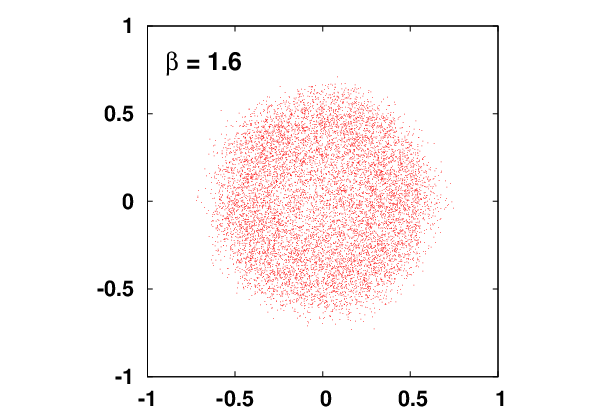
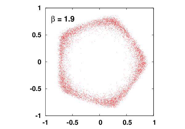
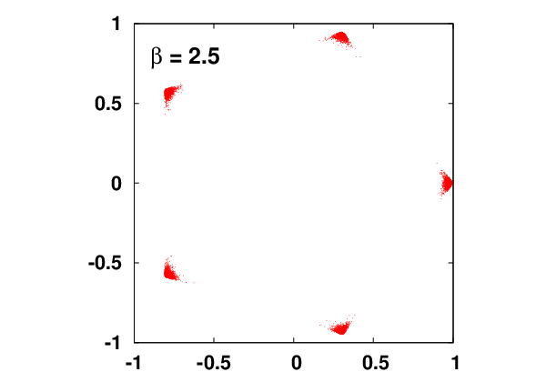
A clear indication of the three-phase structure emerges from the inspection of the scatter plot of the complex magnetization $M_{L}$ at different values of $\beta$: as we move from low to high $\beta$, we observe the transition from a disordered phase (uniform distribution around zero) through an intermediate phase (ring distribution) up to the ordered phase ($N$ isolated spots), as Fig. 1 shows for the case of $Z(5)$ on a $16^{2}\times 2$ lattice.

The first and most important numerical task is to determine the value of the two critical couplings in the thermodynamic limit, $\beta_{c}^{(1)}$ and $\beta_{c}^{(2)}$, that separate the three phases. To this aim we have adopted several methods, which we list here:

• •

  Methods for the determination of $\beta_{\rm c}^{(1)}$:

  (a) locate the position $\beta_{\rm pc}^{(1)}(L)$ of the peak of the susceptibility $\chi_{L}^{(M)}$ of the complex magnetization $|M_{L}|$ on lattices with various spatial size and find $\beta_{\rm c}^{(1)}$ by a fit with the following scaling function, dictated by the essential scaling:

  $$\beta^{(1)}_{\rm pc}=\beta^{(1)}_{\rm c}+\frac{A}{(\ln L+B)^{\frac{1}{\nu}}}\quad,$$

  (18)

  taking $\nu$ equal to 1/2;

  (b) estimate the crossing point of the curves giving the behavior of the Binder cumulant $U_{L}^{(M)}$ versus $\beta$ on lattices with different spatial size $L$ or, alternatively, search for the value of $\beta_{\rm c}^{(1)}$ which optimizes the overlap of these curves when they are plotted against $(\beta-\beta_{\rm c}^{(1)})(\ln L)^{1/\nu}$, with $\nu$ fixed at 1/2;

  (c) consider the helicity modulus $\Upsilon$ near the phase transition and define $\beta_{\rm pc}^{(1)}(L)$ as the value of $\beta$ such that $\eta(\beta)\equiv 1/(2\pi\beta\Upsilon)=1/4$ on the lattice with spatial size $L$ [25], then find $\beta_{\rm c}^{(1)}$ by a fit with the scaling function

  $$\beta^{(1)}_{\rm pc}=\beta^{(1)}_{\rm c}+\frac{A}{\ln L+B}\;,$$

  (19)

  valid under the assumption that the phase transition belongs to the $XY$ universality class.

• •

  Methods for the determination of $\beta_{\rm c}^{(2)}$:

  (d) same as the method (a) using instead the susceptibility $\chi_{L}^{(S)}$ of the population $S_{L}$;

  (e) same as the method (b) using instead simultaneously the Binder cumulant $B_{4}^{(M_{R})}$ and the order parameter $m_{\psi}$.

As an illustration of the methods (a) and (d), we show in Figs. 2 and 3 the behavior of $M_{L}$ (and of its susceptibility) and that of $S_{L}$ (and of its susceptibility) versus $\beta$ in $Z(7)$ on lattices with $N_{t}=2$ and $L$ ranging from 128 to 2048. In Table 2 we summarize all the values of $\beta_{\rm pc}^{(1)}(L)$ and $\beta_{\rm pc}^{(2)}(L)$ found in this work for the application of methods (a) and (d) in $Z(N)$ with $N=5,7$ for $N_{t}=2,4$.

As an illustration of the method (b), we show in Fig. 4 the behavior of $U^{(M)}_{L}$ versus $\beta$ in $Z(7)$ on lattices with $N_{t}=2$ and $L$ ranging from 128 to 2048. Similarly, as an illustration of the method (e), we show in Figs. 5 and 6 the behavior of $B_{4}^{(M_{R})}$ and of $m_{\psi}$ versus $\beta$ in $Z(5)$ on lattices with $N_{t}=4$ and $L$ ranging from 128 to 2048.

As an illustration of the method (c), we show in Fig. 7 the behavior of the helicity modulus $\Upsilon$ versus $\beta$ along with the line $\Upsilon=1/(2\pi\beta\eta),\ \eta=1/4$, describing pseudocritical points, in $Z(5)$ and in $Z(7)$ on lattices with $N_{t}=2,4$ and several values of the spatial extension $L$. For larger values of $L$ only the points around the intersection were simulated.

Finally, we report in Table 3 the determinations of the critical couplings $\beta_{\rm c}^{(1)}$ and $\beta_{\rm c}^{(2)}$ in $Z(N)$ with $N$=5 and 7 for $N_{t}$=2 and 4, specifying the adopted method.

Once critical couplings have been estimated, we are able to extract some critical indices and check the hyperscaling relation.

We start the discussion from the first transition. According to the standard finite-size scaling (FSS) theory, the equilibrium magnetization $|M_{L}|$ at criticality should obey the relation $|M_{L}|\sim L^{-\beta/\nu}$, if the spatial extension $L$ of the lattice is large enough ²² 2 The symbol $\beta$ here denotes a critical index and not, obviously, the coupling of the theory. In spite of this inconvenient notation, we are confident that no confusion will arise, since it will be always clear from the context which $\beta$ is to be referred to.. Therefore, we fit data of $|M_{L}|$ at $\beta^{(1)}_{\rm c}$ on all lattices with size $L$ not smaller than a given $L_{\rm min}$ with the scaling law

where a non-zero value for $r$ takes into account the possibility of logarithmic corrections [26, 27].

The FSS behavior of the susceptibility $\chi^{(M)}_{L}$ is given by $\chi^{(M)}_{L}\sim L^{\gamma/\nu}$, where $\gamma/\nu=2-\eta$ and $\eta$ is the magnetic critical index. Therefore we fit data of $\chi^{(M)}_{L}$ at $\beta^{(1)}_{\rm c}$ on all lattices with size $L$ not smaller than a given $L_{\rm min}$ according to the scaling law

As the value of the critical coupling $\beta^{(1)}_{\rm c}$ we use the central value of the determination from the method (b) (see Table 3).

The results of the fits are summarized in Tables 4, 5, 6, 7, for the cases of $Z(5)$ with $N_{t}$=2, $Z(5)$ with $N_{t}$=4, $Z(7)$ with $N_{t}$=2 and $Z(7)$ with $N_{t}$=4, respectively. The reference value for the index $\eta$ at this transition is 1/4, whereas the hyperscaling relation to be fulfilled is $\gamma/\nu+2\beta/\nu=d=2$.

The procedure for the determination of the critical indices at the second transition is similar to the one for the first transition, with the difference that the fit with the scaling laws Eqs. (20) and (21) is to be applied to data of the rotated magnetization, $M_{R}$, and of its susceptibility, $\chi_{L}^{(M_{R})}$, respectively. As the value of the critical coupling $\beta^{(2)}_{\rm c}$ we use the one determined from the method (e) (see Table 3).

The results of the fits are summarized in Tables 8, 9, 10, 11, for the cases of $Z(5)$ with $N_{t}$=2, $Z(5)$ with $N_{t}$=4, $Z(7)$ with $N_{t}$=2 and $Z(7)$ with $N_{t}$=4, respectively. The reference value for the index $\eta$ at this transition is $4/N^{2}$, i.e. $\eta=0.16$ for $N=5$ and $\eta=0.0816..$ for $N=7$, whereas the hyperscaling relation to be fulfilled is $\gamma/\nu+2\beta/\nu=d=2$.

A general comment is that in many of the cases we investigated both $d$ and $\eta$ at the two critical points slightly differ from the expected values, though these differences cancel to a large extent if we define $\eta$ as $2\beta/\nu$.

There is an independent method to determine the critical exponent $\eta$, which does not rely on the prior knowledge of the critical coupling, but is based on the construction of a suitable universal quantity [28, 21]. The idea is to plot $\chi_{L}^{(M_{R})}L^{\eta-2}$ versus $B_{4}^{(M_{R})}$ and to look for the value of $\eta$ which optimizes the overlap of curves from different volumes. This method is illustrated in Fig. 8 for the case of $Z(7)$ with $N_{t}=4$: for $\eta=0.25$ the overlap is optimal in the lower branch of the curves, corresponding to the region of the first transition, while per $\eta=0.0816\simeq 4/7^{2}$ the overlap is optimal in the upper branch. Another option is to plot $M_{R}L^{\eta/2}$ versus $m_{\psi}$, which leads to overlapping curves for $\eta$ fixed at the value of the second phase transition, as illustrated in Fig. 9 for the case of $Z(7)$ with $N_{t}=2$ and $N_{t}=4$.

To produce further evidence in favor of the fact that the phase transitions investigated so far are both of infinite order, we have calculated the mean link energy $E$ and the specific heat $C$ around the transitions in $Z(5)$ and in $Z(7)$ with $N_{t}$=2 and $N_{t}=4$ (see Fig. 10 for the case of $Z(7)$ with $N_{t}=4$, for example). In all cases the dependence of $E$ and $C$ on $\beta$ is continuous, so that first and second order transitions are ruled out.

References

- [1] G. Bhanot and M. Creutz, Phys. Rev. D 21 (1980) 2892.
- [2] A. Polyakov, Nucl. Phys. B 120 (1977) 429; T. Banks, J. Kogut, R. Myerson, Nucl. Phys. B 121 (1977) 493; M. Göpfert, G. Mack, Commun. Math. Phys. 81 (1981) 97.
- [3] B. Svetitsky, L. Yaffe, Nucl. Phys. B 210 (1982) 423.
- [4] V. Berezinskii, Sov. Phys. JETP 32 (1971) 493.
- [5] J. Kosterlitz, D. Thouless, J. Phys. C 6 (1973) 1181.
- [6] J. Kosterlitz, J. Phys. C 7 (1974) 1046.
- [7] N. Parga, Phys. Lett. B 107 (1981) 442.
- [8] O. Borisenko, Critical behaviour of 3D U(1) LGT at finite temperature, PoS LAT 2007 (2007) 170.
- [9] O. Borisenko, M. Gravina, A. Papa, J. Stat. Mech. 2008 (2008) P08009.
- [10] O. Borisenko, R. Fiore, M. Gravina, A. Papa, J. Stat. Mech. 2010 (2010) P04015.
- [11] F.Y. Wu, Rev. Mod. Phys. 54 (1982) 235.
- [12] S. Elitzur, R.B. Pearson, J. Shigemitsu, Phys. Rev. D 19 (1979) 3698.
- [13] M. B. Einhorn, R. Savit, and E. Rabinovici, Nucl. Phys. B 170 (1980) 16.
- [14] C.J. Hamer, J.B. Kogut, Phys. Rev. B 22 (1980) 3378.
- [15] B. Nienhuis, J. Statist. Phys. 34 (1984) 731.
- [16] L.P. Kadanoff, J. Phys. A 11 (1978) 1399.
- [17] J.L. Cardy, J. Phys. A 13 (1980) 1507.
- [18] J. Fröhlich, T. Spencer, Commun. Math. Phys. 81 (1981) 527.
- [19] Y. Tomita, Y. Okabe, Phys. Rev. B 65 (2002) 184405.
- [20] O. Borisenko, G. Cortese, R. Fiore, M. Gravina, A. Papa, Critical properties of the two-dimensional Z(5) vector model, PoS LATTICE 2010 (2010) 274 [arXiv:1101.0512 [hep-lat]].
- [21] O. Borisenko, G. Cortese, R. Fiore, M. Gravina and A. Papa, Phys. Rev. E 83 (2011) 041120.
- [22] O. Borisenko, G. Cortese, R. Fiore, M. Gravina, A. Papa, Critical properties of 2D Z(N) models for , PoS LATTICE 2011 (2011) 304 [arXiv:1110.6385 [hep-lat]].
- [23] O. Borisenko, V. Chelnokov, G. Cortese, R. Fiore, M. Gravina, A. Papa, Phys. Rev. E 85 (2012) 021114.
- [24] M. Billò, M. Caselle, A. D’Adda, Int. J. Mod. Phys. A 12 (1997) 5753.
- [25] A. Yamagata and I. Ono, J. Phys. A24 (1991) 265.
- [26] R. Kenna and A. C. Irving, Nucl. Phys. B 485 (1997) 583.
- [27] M. Hasenbusch, J. Phys. A 38 (2005) 5869.
- [28] D. Loison, J. Phys.: Condens. Matter 11 (1999) L401.
- [29] E. Domany, D. Mukamel, A. Schwimmer, J. Phys. A 13 (1980) L311.