A close look into the excluded volume effects within a double layer
Abstract
We explore the effect of steric interaction on the ionic density distribution near a charged hard wall. For weakly charged walls, small particles, and monovalent ions the mean-field Poisson-Boltzmann equation provides an excellent description of the density profiles. For large ions and large surface charges, however, deviations appear. To explore these, we use the density functional theory. We find that local density functionals are not able to account for steric interactions near a wall. Based on the weighted density approximation we derive a simple analytical expression for the contact electrostatic potential which allows us to analytically calculate the differential capacitance of the double layer.
I Introduction
The standard Poisson-Boltzmann equation (PB) is accurate for dilute aqueous solutions containing small monovalent ions. The first approximation of the PB theory is the mean-field account of the electrostatic interactions, where the discrete nature of ions is neglected and each ion interacts with the mean-potential generated by the local charge density distribution according to the Coulomb law, , where is the dielectric constant. This description clearly ignores ionic correlations. The other approximation within the PB theory is the lack of internal structure of each ion: an ion is a point in space characterized only by its charge. Under this reduced description the ions F-, Cl-, and NO are indistinguishable, although their size [1] and polarizability [2] are obviously different. The PB description, therefore, breaks down when the above reductions can no longer be justified. In the present work we consider the weakly correlated limit so that the mean-field description of electrostatics holds, but we go beyond the standard PB equation by including the nonelectrostatic excluded volume effects [1]. In aqueous solutions the excluded volume interactions are further increased on account of hydration, the binding of water molecules to ions, so that the effective ionic radii are larger than the crystallographic ones [3, 4, 5]. Another effect of hydration, related directly to electrostatics, is the dielectric decrement [6, 7, 8] associated with the decrease of the medium dielectric constant on account of polarization saturation of a solvent constituting the hydration shell. In the present work we do not consider this effect and focus strictly on the non-electrostatic excluded volume effects.
The excluded volume effects reorganize the double layer so that a density profile is no longer monotonically decreasing, but it acquires oscillatory structure reflecting molecular composition of an electrolyte [9]. Clearly, the modifications of the density profile lead to modified electrostatic properties. In the present study we take a close look into the excluded volume effects where ions are represented as hard spheres with the same diameter, the so-called, restricted primitive model. Not only do we investigate how the ionic system responds to these effects under various conditions, but also how well various theories reproduce this behavior. The hard-sphere interactions lead to the nonlocal effects, demanding nonlocal functionals to account for the oscillatory structure in the density profile. The nonlocal treatments, such as the density functional theory (DFT), can be computationally demanding if the system is sufficiently complex. Frequently in electrostatics, a variant of the local density approximation (LDA) is used, where the ideal gas entropy is substituted by that of the lattice-gas leading to the modified Poisson-Boltzmann equation (MPB) [11, 10]. With growing popularity of the MPB as a simple and tractable model, we feel that a careful and systematic study of this method is still lacking. First of all, the MPB is a local theory inappropriate for moderately and highly inhomogeneous fluids. Furthermore, even as a theory of a homogeneous fluid it already fails at predicting the correct second virial term. We consider another variant of the LDA based on the scaled particle theory (SPT). Surprisingly, although highly accurate for treating homogeneous fluids, it is less accurate than the MPB, which is unreliable for homogeneous fluids. We compare all the results against the nonlocal fundamental measure density functional theory [12]. Our main focus is the region near and at the contact with the wall, where exact thermodynamic relations are known. We investigate the scaling properties of the contact quantities and propose an analytical fit to the DFT data that permits an accurate prediction of these quantities, without resorting to numerical computations involving the entire region.
Throughout the paper we make frequent use of the initials: DFT, LDA, MPB, and SPT. To avoid confusion we give a quick account of each. DFT always refers to the fundamental measure density functional theory as originally derived by Rosenfeld [12]. This is the only nonlocal theory used in this work. LDA refers to the general class of approximations where a density functional is defined locally based on a free energy of a homogeneous fluid. MPB is the special example of the LDA, when the excluded volume effects are represented as that of a homogeneous lattice gas [11]. And the SPT stands for the scaled particle theory and refers to the theoretical approach based on scaling a particle size [13, 14, 15, 16]. We use SPT to refer to another LDA approximation based on the SPT results for a uniform fluid. In the paper two LDA approximations will be considered: the MPB and the SPT.
The paper is organized as follows. In Section II we discuss a reversible work of inserting a test particle into a hard sphere fluid, , and emphasize its nonlocal character by deriving the exact result for inserting a point particle into a hard-sphere fluid. We then introduce the fundamental density functional theory as an accurate nonlocal treatment of the hard-sphere interactions. In Section III we review the contact value theorem and explore its implications for the counterion distribution near a hard charged surface. We point out that the LDA theories lead to contact relations different from the exact contact value theorem. This is the result of representing the overcrowding in the double-layer as the density ”saturation”. In Section IV we investigate the scaling of the quantity , which represents the reversible work of brining the uncharged fluid particle from the bulk into contact with the wall. We propose the analytical formula for that fits the DFT data points. In Section V we apply this formula to calculate the surface potential and the differential capacitance. Section VI finalizes this work with the concluding remarks.
II Preliminaries
We write the free energy functional as having three separate contributions,
| (1) |
the ideal gas contribution,
| (2) |
the mean-field electrostatic interactions,
| (3) |
and the excluded volume contributions, , where all ions are taken to have the same diameter . denotes a fixed charge of a macromolecule and in the present work we consider a charged wall, , where is the surface charge. is the charge density of mobile ions, where is the charge of an ion species and is the number of all ionic species. Finally, is the de Broglie wavelength. The equilibrium density minimizes the grand potential functional,
| (4) |
with respect to a density distribution, , and leads to
| (5) |
where is the mean electrostatic potential, , and is the bulk density of an ion species .
Physically, represents the reversible work of inserting a test particle at position into a hard-sphere fluid [13, 14, 15, 16]. If the system has a wall, the insertion performed far from the wall, is identical with the excess (over the ideal gas) chemical potential. Alternatively, can be seen as a depletion interaction: as a particle approaches a hard-wall, it feels itself being pushed towards the wall by the other particles. Application of the Poisson equation, , leads to a kind of modified Poisson-Boltzmann equation,
| (6) |
where the surface charge is determined by the boundary conditions at a charged wall,
In order to obtain the potential, one still needs some kind of closure for that will determine the excluded volume effects.
II.1 insertion of a point particle – the exact case
is a nonlocal quantity. To see the origins of the non-locality we consider a simple case where the insertion work can be expressed as an exact density functional. The case we refer to is the reversible work of inserting a point test particle into a hard-sphere fluid, . The range of the hard-core interaction between the test point particle and the fluid hard-spheres is half the diameter, . The reversible work is related to the insertion probability, . For a given instantaneous configuration of a hard sphere fluid, the space is either occupied or is empty. The point particle can be inserted into the empty space between the hard spheres. The instantaneous insertion probability, , is either zero, if we hit on an occupied space, or one, if a cavity is found,
| (7) | |||||
where is the density operator, is the total number of fluid particles, and is the Heaviside step function. Averaging over all the configurations, we obtain
| (8) |
The reversible work of inserting a point particle at position is
| (9) |
The non-locality of is already evident in this simple example and shows that the work of inserting a point particle depends on the weighted average of the inhomogeneous density distribution. The extent of the nonlocality is determined by the range of the hard-core interaction. To obtain an expression for , a reversible work associated with expanding a point particle to diameter has to be considered, and constitutes only a part of the entire quantity . For the homogeneous fluid, this procedure leads to the scaled particle theory (SPT) [13], in which the work of expansion to finite diameter is interpolated between the two exact limits, and , where is the range of the hard sphere interaction between a test and a fluid particle. For an inhomogeneous fluid the derivation is more involved [12].
II.2 density functional theory
The ideas of the SPT applied to inhomogeneous fluids lead to the formulation of the fundamental measure density functional theory (DFT) [12]. The DFT approximates the excess free energy due to the hard-sphere interactions through the free energy contribution, , where
| (10) |
The hard sphere contributions are locally represented through weighted densities, instead of a physical density, as is the case for the LDA approximation,
| (11) |
with denoting a weight function [12, 17]. There are five weight functions which are obtained through decomposition of the Mayer- function into convolution products [18]. The two of the weight functions are vector quantities and represent a distribution of normal to the sphere surface vectors. In the uniform fluid they have no contribution. The weight functions are given below,
| (12) |
and , , and , where . Since we assume the size of all ions to be the same, the weight functions are the same for all the ionic species. The insertion work is defined as the functional derivative of the excess part of free energy,
| (13) |
The DFT theory presented above accurately captures the dimensional crossover when the 3d fluid is confined to a quasi-2d space [19] — if a degree of freedom is completely eliminated in the transverse direction, a 2d fluid is accurately recovered.

II.3 local density approximation (LDA)
Although highly accurate, see Fig. (1), the numerical implementation of the fundamental measure density functional theory is quite involved. To simplify the calculations, local density approximations (LDA) have often been invoked. Within the LDA, the thermodynamic relations derived for a homogeneous fluid are applied locally to an inhomogeneous situation. For example, within the LDA the insertion probability is supposed to be a function of the local density and is identified with the ”local” excess chemical potential, . Clearly the specific form of the LDA will depend on the approximate form of . The MPB [11] relies on derived from the lattice-gas description of electrolyte, , where is the packing fraction. The SPT expression is .
III the contact value theorem
In this work we focus on the region at a contact with a charged wall. In this region the excluded volume effects are most pronounced since the ion concentration is highest, and for many problems the contact quantities are of primary interest. This is the case for calculation of the differential capacitance [21], or the estimation of the strength of the electrostatic interactions between colloids trapped at an interface [22]. The theoretical investigation in this region is facilitated by the existence of exact thermodynamic relations. This section reviews some analytical results valid at a contact with a wall. Throughout the paper we make frequent use of either the subscript or the superscript to indicate that a quantity is taken at contact with the wall. In the same way we use to indicates bulk values. We remind that the charge and number density are and , respectively. Consequently, the bulk and contact value of the number density is and , respectively.
III.1 exact results
The simplest expression of the contact value theorem relates the bulk pressure to the average momentum transferred at the hard-wall: , where is the fluid density at the contact with the wall. If the hard-wall has a surface charge and the particles are hard-spheres with a central charge, then the contact value theorem takes the form [23],
| (14) |
Within the DFT formalism the pressure is given according to the scaled particle theory. This result is a highly accurate approximation and the contact value theorem according to the DFT is essentially exact. The contact value relation is the result of the mechanical force balance condition,
| (15) |
where the thermodynamic force on the left-hand side is counterbalanced by the electrostatic force and the depletion force due to the collisions with other fluid particles on the right-hand side.
The explicit expression for the contact density, using Eq. (5), is
| (16) |
where we have introduced the quantity
| (17) |
representing the reversible work expanded to bringing a hard-sphere particle (with no electric charge) from the bulk electrolyte to the wall. This is not to say that is independent of electrostatic properties. The work of bringing an uncharged hard-sphere to the wall depends on the ionic distribution within the double-layer that depends on the electrostatic interactions. Substituting the density in Eq. (16) into the contact value theorem gives
| (18) |
For the case , is known exactly and is determined by the bulk quantities and the surface charge. The standard PB equation describes this scenario. A finite modifies the contact potential. signifies that it is easier to insert a particle far away from the wall than at the contact. This is intuitive because near the wall counterions are in excess. Consequently the contact potential is larger than that obtained from the standard PB equation — steric interactions deplete some ions from the first layer making it more difficult to neutralize the wall charge. On the other hand, signifies that it is easier to insert a particle at the wall than far from it. Although this seems counterintuitive, it can occur at low values of the surface charge and/or large . To see this we consider the limit ,
| (19) |
In this limit, is always negative (since ), and the larger the bulk packing fraction , the larger will be the modulus of . At large ionic concentrations – such as, for example, found in ionic liquids – the range of where is negative can be significant. In Fig. (2) we plot as a function of for different values of the surface charge. The crossover where changes sign to negative is pushed to larger as becomes larger. Eventually the crossover is suppressed as passes the freezing transition (at ).

III.2 local density approximation (LDA)
Within the local density approximation the insertion work is a local quantity,
| (20) |
and the force density due to the hard-sphere interactions can be related to the gradient of a local pressure,
| (21) |
The force balance equation in Eq. (15) becomes
| (22) |
leading, after integrating over a half-space, to the contact relation,
| (23) |
where is the local pressure at contact with the wall. The notion of a local pressure can be somewhat misleading, since the pressure is normally associated with bulk properties. It is only sensible to talk about a local pressure within the framework of a local density approximation.
Going back to the exact contact value theorem in Eq. (14) shows that the correct thermodynamic result is obtained only if . Paradoxically, if one tries to improve on this result and go beyond the PB description by including an excess free energy due to electrostatic or steric correlations using a LDA formalism, one obtains less accurate contact value density than if the correlations are neglected altogether. The unphysical contact value relation for the LDA treatment is a consequence of an unphysical density profile. The LDA approximation fails to capture the oscillating discrete structure of a fluid, see Fig. (3).

As seen in that figure, the LDA approximations account for overcrowding through ”density saturation”, while a realistic description shows overcrowding as layering of a fluid near a wall. It is tempting to assume that the ”saturation” observed in a density for the LDA models represents a weighted rather than a physical density profile,
| (24) |
where is some weight function, so that oscillations are completely smoothed out. Such conjecture, however, entails that obtained from the LDA is also not physical but only a weighted quantity. We, therefore, consider that all quantities produced by the LDA are what they are, and that the saturation of a density profile is an artifact of the LDA treatment. To test accuracy of the LDA one should rather consider other quantities such as , which is of direct interest to most problems of electrostatics.
Below we look into details of two LDA models. As mentioned earlier, the SPT results are highly accurate for homogeneous fluids, producing the exact second virial coefficient. Furthermore, the third and higher order virial coefficients are very accurate,
| (25) |
On the other hand, the lattice-gas model (from which the MPB is derived) already fails at the second virial coefficient,
| (26) |
and is unfit for treating homogeneous fluids.
On the other hand, when the LDA is applied to inhomogeneous fluids, it is hard to predict what will happen. In Fig. (4) we plot the contact potential for various models. First we note that the difference between the PB and the DFT results. The finite size effects lead to an increase of the surface potential, and the larger the surface charge, the larger the discrepancy, since more counterions are crowded into the double-layer. Next we discuss the LDA models. The MPB model underestimates while the LDA based on the SPT overestimates the DFT result.

We next consider the quantity as defined in Eq. (17). As shown in Fig. (5) the MPB reproduces this quantity better than the STP. The advantage of the MPB model is its analytical tractability, and according to this model yields a very simple expression,
| (27) |
with parabolic in .

IV Scaling of the quantity
All the calculations in this work are carried out for the symmetric salt, so that the bulk number density is , where denotes the bulk salt concentration. In this part of the study we investigate the scaling of the quantity . is a function of three dimensionless variables: , , and , corresponding to volume, surface, and length, respectively. represents the packing fraction of counterions projected on a 2d plane. The 2d solid phase transition is at , and the maximum possible packing fraction is at . If , potentially all the counterions can collapse onto the charged surface, if attraction is sufficiently strong (although would involve a phase transition as well). If, on the other hand, , collapse onto a single plane is prevented and a second fluid layer must form. In the reduced units, the contact value theorem is
| (28) |
where is the reduced potential, and is the volume of a single fluid particle.
According to the LDA, is a function of two independent parameters, and . Later, as we investigate for various parameters using the DFT, we do not find this reduced description to be confirmed, and we conclude that it is an artifact of the LDA. Furthermore, this implies that the scaling of the contact potential according to the LDA description is described by two independent parameters. The two parameter scaling of the LDA can be ascertained from the contact relation in Eq. (23).
IV.1 dilute limit
To simplify things we first consider the dilute limit, so as to suppress the contributions from the bulk eliminating the dependence on , . The main results are in Fig. (6) and Fig. (7). The figures show the scaling behavior of . The general observation is that the scaling with the surface charge is stronger than that with the Bjerrum length. This can be understood since the surface charge controls both the interactions between the surface and counter charges and the counterion concentration. On the other hand, the Bjerrum length regulates only the strength of the ionic interactions.

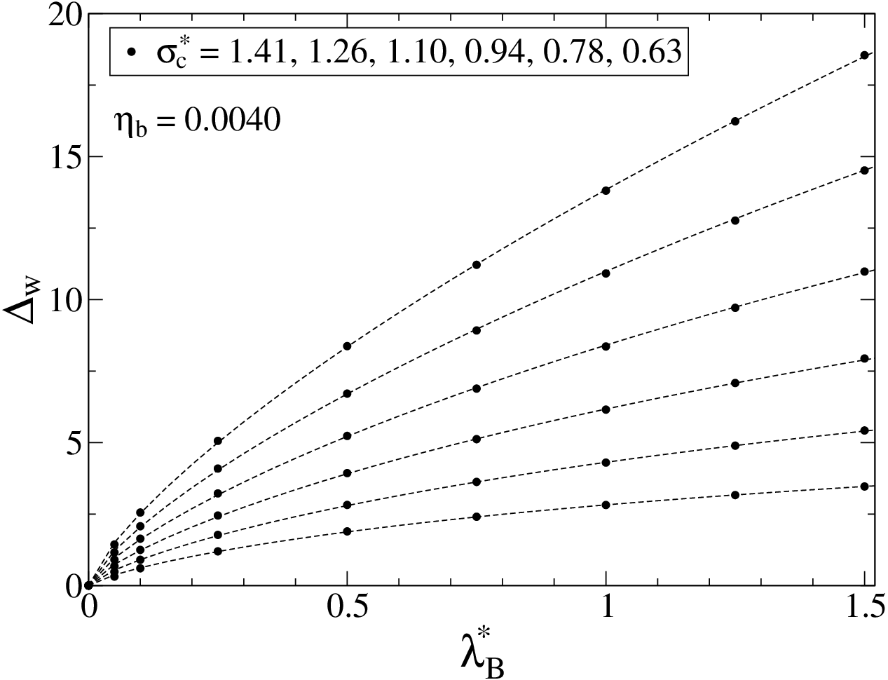
Our aim is to propose a fit which reproduces the scaling of . The desirable procedure would be to suggest an expression based on a physically motivated model. Unfortunately, an accurate physically motivated fit could only be found for a limited range. To accurately parametrize the entire range we had to resort to a fitting procedure where the choice of a functional form was based on simplicity and convenience. The following functional form was found convenient, . Fully parametrized, this form reads
| (29) | |||||
The accuracy of this fit is demonstrated in Figs. (6) and Fig. (7) in comparison to the DFT data points. We also compare this formula with the simple expression from the MPB model in Eq. (27) which in reduced units reads
| (30) |
There is a curious similarity between the square term in our fit and the coefficient in the MPB expression. If this similarity is more than coincidental, it would suggest that although reduced, the MPB description accurately captures some aspects of the hard-sphere interactions.
IV.2 finite concentrations
We now turn to investigate the contributions of finite concentrations. We suggest the following formula,
| (31) |
so that as a function of is merely shifted by the quantity . This fit is suggested by Fig. (8) where we compare for finite with that for a dilute limit. In the relevant regime as a function of is offset by a value independent of . We find the following accurate fit to the function ,
| (32) |
We subtract from so that the quantity is always positive, see Eq. (19) and Fig. (2). To ensure that , so that for all values of , we apply the form,
| (33) |

V applications
We now have the complete expression for ,
| (34) |
where is given in Eq. (33). To obtain the contact potential, we insert into Eq. (28) to get
| (35) |
In Fig. (9) and Fig. (10) we compare the exact DFT results for the contact potential with the ones obtained using the analytical scaling function Eq. (35) and with the predictions of the MPB model.


The scaling form derived in the present paper agrees very well with the contact potential obtained using the exact DFT, even at densities all the way to the solid phase transition. For largest particle sizes, Fig. (10) shows that the scaling function slightly disagrees with the DFT results. This happens when and a third layer of condensed counterions starts to form.
A quantity that is of particular interest for electrochemistry is the differential capacitance of the double-layer [21],
The standard PB result gives
which is the, so-called, Gouy-Chapman capacitance. is the inverse Debye length. At low this formula works well, but as increases, steric repulsion lowers the capacitance as counterions are prevented from accumulating near the electrode, leading to a ”camel-shaped” curve of Fig. (11). The scaling function derived in the present paper allows us to easily calculate the differential capacitances, which once again are in a very good agreement with the DFT.

VI Conclusion
We have investigated the effects of steric interactions on the ionic distribution and electrostatic properties near a charged hard wall. We have specifically focused on the reversible work required to bring a hard spherical particle (with no electric charge) from the bulk to the wall, . The quantity is nonlocal and it controls the steric effects in the double-layer. Typically . This implies that the overcrowding near a wall causes the depletion of counterions away from the wall, leading to the increased contact potential. The less common case, , represents the situation where counterions are forced from the dense bulk toward the wall. This effect decreases the value of the contact potential.
We have also studied the scaling behavior of calculated using the nonlocal DFT theory. We expected that the careful look into the scaling behavior can reveal a simple underlying mechanism. Unfortunately, no simple model could cover the entire domain. Instead we proposed a functional form to fit the DFT data points for . Such a fit allows for simple and accurate calculation of electrostatic properties at contact with the wall without resorting to numerical schemes of an entire region.
Finally, we have explored the discrepancies between the LDA and exact description. The LDA description shows that depends on two free parameters, in comparison to the three parameters given by full physical description (DFT). Another artifact of the LDA is the ”saturation” seen in a density profile rather than oscillations due to layering. This saturation effect leads to unphysical contact value relation. For various LDA models, we find that the MPB based on the lattice-gas model is more accurate than the LDA based on the SPT theory, which for treating a uniform fluid is extremely accurate. This indicates that some cancellation of errors is at work.
We remind that our analysis is limited to the weak-coupling limit, where electrostatic interactions are accurately captured by the mean-field treatment. To accurately account for the correlations together with the hard-sphere interactions remains a great challenge. It is our hope to treat the strong-coupling limit of the hard-sphere ions in the future.
Acknowledgements.
This work was partially supported by the CNPq, Fapergs, INCT-FCx, and by the US-AFOSR under the grant FA9550-09-1-0283. We thank Alexandre Pereira dos Santos for furnishing us with the simulation data in Fig. (1).References
- [1] Y. Levin, Rep. Prog. Phys. 65, 1577 (2002).
- [2] D. Frydel, J. Chem. Phys. 134, 234704 (2011).
- [3] E. R. Nightingale, J. Phys. Chem. 63, 1381 (1959).
- [4] Y. Levin, A. P. dos Santos, A. Diehl, Phys. Rev. Lett. 103, 257802 (2009); A. P. dos Santos, A. Diehl, and Y. Levin, Langmuir 26, 10778 (2010).
- [5] I. Kalcher, J. C. F. Schulz, and J. Dzubiella, Phys. Rev. Lett. 104, 097802 (2010).
- [6] E. Glueckauf, Trans. Faraday Soc. 60, 1637 (1964)
- [7] D. Ben-Yaakov, D. Andelman, and R. Podgornik, J. Chem. Phys. 134, 074705 (2011).
- [8] A. Levy, D. Andelman, H. Orland, http://arxiv.org/abs/1201.6081v1.
- [9] D. Antypov, M. C. Barbosa, and C. Holm, Phys. Rev. E 71, 061106 (2005).
- [10] M. Z. Bazant, M S Kilic, B Storey, and A Ajdari, Adv. Colloid Interface Sci., 152, 48 (2009).
- [11] I. Borukhov, D. Andelman, H. Orland, Phys. Rev. Lett. 79, 435 (1997).
- [12] Y. Rosenfeld, Phys. Rev. Lett. 63, 980 (1989).
- [13] H. Reiss, H. L. Frisch, J. L. Lebowitz, J. Chem. Phys. 31, 369 (1959).
- [14] B. Widom, J. Chem. Phys. 39, 2808 (1963).
- [15] F. C. Andrews, J. Chem. Phys. 62, 272 (1974).
- [16] M. Heying and D. S. Corti, J. Phys. Chem. B 108, 19756 (2004). D. W. Siderius and D. S. Corti, J. Chem. Phys. 127, 144502 (2007).
- [17] Roland Roth, J. Phys.: Condens. Matter 22, 063102 (2010); R. Evans, Lecture notes at 3rd Warsaw School of Statistical Physics, Kazimierz Dolny, June 2009 pp. 43-85 Warsaw University Press (2010).
- [18] S. Korden, http://arxiv.org/abs/1111.5222.
- [19] Y. Rosenfeld, M. Schmidtz, H. Löwen, and P. Tarazona, J. Phys.: Condens. Matter 8, L577 (1996).
- [20] A. Diehl, A. P. dos Santos, Y. Levin, J. Phys.: Condens. Matter 24, 284115 (2012).
- [21] A. A. Kornyshev, J. Phys. Chem. B 111, 5545 (2007).
- [22] D. Frydel, M. Oettel, S. Dietrich, Phys. Rev. Lett. 99, 118302 (2007); D. Frydel and M. Oettel, Phys. Chem. Chem. Phys. 13, 4109 (2011).
- [23] D. Henderson, L. Blum, J. L. Lebowitz, J. Electroanal. Chem. 102, 315 (1979).
- [24] A. P. dos Santos, A. Diehl, and Y. Levin, J. Chem. Phys. 130, 124110 (2009).
- [25] D. Henderson, S. Lamperski, Z. Jin, and J. Wu, J. Phys. Chem B 115, 12911 (2011).