Synchronization and Power Sharing
for Droop-Controlled Inverters in Islanded Microgrids^footnoteinfo

A microgrid is a low-voltage electrical network, heterogeneously composed of distributed generation, storage, load, and managed autonomously from the larger primary network. Microgrids are able to connect to the wide area electric power system (WAEPS) through a Point of Common Coupling (PCC), but are also able to “island” themselves and operate independently. Energy generation within a microgrid can be highly heterogeneous, any many these sources generate either variable frequency AC power (wind) or DC power (solar), and are therefore interfaced with a synchronous AC microgrid via power electronic devices called DC/AC (or AC/AC) power converters, or simply inverters. In islanded operation, inverters are operated as voltage sourced inverters (VSIs), which act much like ideal voltage sources. It is through these VSIs that actions must be taken to ensure synchronization, security, power balance and load sharing in the network.

Literature Review: A key topic of interest within the microgrid community is that of accurately sharing both active and reactive power among a bank of inverters operated in parallel. Such a network is depicted in Figure 1, in which each inverter transmits power directly to a common load.

Although several control architectures have been proposed to solve this problem, the so-called “droop” controllers have attracted the most attention, as they are ostensibly decentralized. The original reference for this methodology is [6], where Chandorkar et. al. introduce what we will refer to as the conventional droop controller. For inductive lines, the droop controller attempts to emulate the behavior of a classical synchronous generator by imposing an inverse relation at each inverter between frequency and active power injection [18]. Under other network conditions, the controller takes different forms [16, 33, 35]. Some representative references for the basic methodology are [30, 2, 21, 22, 20] and [17]. Small-signal stability analyses for two inverters operating in parallel are presented under various assumptions in [10, 11, 23, 25] and the references therein. The recent work [34] highlights some drawbacks of the conventional droop method. Distributed controllers based on tools from synchronous generator theory and multi-agent systems have also been proposed for synchronization and power sharing. See [26, 27] for a broad overview, and [35, 29, 4, 32] for various works.

Another set of literature relevant to our investigation is that pertaining to synchronization of phase-coupled oscillators, in particular the classic and celebrated Kuramoto model. A generalization of this model considers $n\geq 2$ coupled oscillators, each represented by a phase $\theta_{i}\in\mathbb{S}^{1}$ (the unit circle) and a natural frequency $\Omega_{i}\in\mathbb{R}$. The system of coupled oscillators obeys the dynamics

where $a_{ij}\geq 0$ is the coupling strength between the oscillators $i$ and $j$ and $D_{i}$ is the time constant of the $i^{th}$ oscillator.

Figure 2 shows a mechanical analog of (1), in which the oscillators can be visualized as a group of $n$ kinematic particles, constrained to rotate around the unit circle. The particles rotate with preferred directions and speeds specified by the natural frequencies $\Omega_{i}$, and are connected together by elastic springs of stiffness $a_{ij}$. The rich dynamic behavior of the system (1) arises from the competition between the tendency of each oscillator to align with its natural frequency $\Omega_{i}$, and the synchronization enforcing coupling $a_{ij}\sin(\theta_{i}-\theta_{j})$ with its neighbors. We refer to the recent surveys [1, 28, 12] for applications and theoretic results.

The Frequency-Droop Method: The frequency-droop method constitutes one half of the conventional droop method. For inductive lines, the controller balances the active power demands in the network by instantaneously changing the frequency $\omega_{i}$ of the voltage signal at the $i^{th}$ inverter according to

where $\omega^{*}$ is a rated frequency, ${P}_{\textup{e,$i$}}$ is the active electrical power injection at bus $i$, and $P_{i}^{*}$ is the nominal active power injection. The parameter $n_{i}>0$ is referred to as the droop coefficient.

Limitations of the Literature: Despite forming the foundation for the operation of parallel VSIs, the frequency-droop control law (2) has never been subject to a nonlinear analysis [34]. No conditions have been presented under which the controller (2) leads the network to a synchronous steady state, nor have any statements been made about the convergence rate to such a steady state should one exist. Stability results that are presented rely on linearization for the special case of two inverters, and sometimes come packaged with extraneous assumptions [22, 17]. No guarantees are given in terms of performance. Schemes for power sharing based on ideas from multi-agent systems often deal directly with coordinating the real and reactive power injections of the distributed generators, and assume implicitly that a low level controller is bridging the gap between the true network physics and the desired power injections. Moreover, conventional schemes for frequency restoration typically rely on a combination of local integral action and separation of time scales, and are generally unable to maintain an appropriate sharing of power among the inverters (see Sections 4–5).

Contributions: The contributions of this paper are four-fold. First, we begin with our key observation that the equations governing a microgrid under the frequency-droop controller can be equivalently cast as a generalized Kuramoto model of the form (1). We present a necessary and sufficient condition for the existence of a locally exponentially stable and unique synchronized solution of the closed-loop, and provide a lower bound on the exponential convergence rate. We also state a robustified version of our stability condition which relaxes the assumption of fixed voltage magnitudes and admittances. Second, we show rigorously—and without assumptions on large output impedances or identical voltage magnitudes—that if the droop coefficients are selected proportionally, then power is shared among the units proportionally. We provide explicit bounds on the set of serviceable loads. Third, we propose a distributed “secondary” integral controller for frequency stabilization. Through the use of a distributed-averaging algorithm, the proposed controller dynamically regulates the network frequency to a nominal value, while preserving the proportional power sharing properties of the frequency-droop controller. We show that this controller is locally stabilizing, without relying on the classic assumption of a time-scale separation between the droop and integral control loops. Fourth and finally, all results presented extend past the classic case of a parallel topology of inverters and hold for generic acyclic interconnections of inverters and loads.

Paper Organization: The remainder of this section introduces some notation and reviews some fundamental material from algebraic graph theory, power systems and coupled oscillator theory. In Section 2 we motivate the mathematical models used throughout the rest of the work. In Section 3 we perform a nonlinear stability analysis of the frequency-droop controller. Section 4 details results on power sharing and steady state bounds on power injections. In Section 5 we present and analyze our distributed-averaging integral controller. Finally, Section 7 concludes the paper and presents directions for future work.

Preliminaries and Notation:
Sets, vectors and functions: Given a finite set $\mathcal{V}$, let $|\mathcal{V}|$ denote its cardinality. Given an index set $\mathcal{I}$ and a real valued 1D-array $\{x_{1},\ldots,x_{|\mathcal{I}|}\}$, $\mathrm{diag}(\{x_{i}\}_{i\in\mathcal{I}})\in\mathbb{R}^{|\mathcal{I}|\times|\mathcal{I}|}$ is the associated diagonal matrix. We denote the $n\times n$ identity matrix by $I_{n}$. Let $\boldsymbol{1}_{n}$ and $\boldsymbol{0}_{n}$ be the $n$-dimensional vectors of all ones and all zeros. For $z\in\mathbb{R}^{n}$, define $z^{\perp}\triangleq\{x\in\mathbb{R}^{n}\;|\;z^{T}x=0\}$ and $\boldsymbol{\sin}(z)\triangleq(\sin(z_{1}),\ldots,\sin(z_{n}))^{T}\in\mathbb{R}^{n}$.

Algebraic graph theory: We denote by $G(\mathcal{V},\mathcal{E},A)$ an undirected and weighted graph, where $\mathcal{V}$ is the set of nodes, $\mathcal{E}\subseteq\mathcal{V}\times\mathcal{V}$ is the set of edges, and $A\in\mathbb{R}^{|\mathcal{V}|\times|\mathcal{V}|}$ is the adjacency matrix. If a number $\ell\in\{1,\dots,|\mathcal{E}|\}$ and an arbitrary direction is assigned to each edge $\{i,j\}\in\mathcal{E}$, the node-edge incidence matrix $B\in\mathbb{R}^{|\mathcal{V}|\times|\mathcal{E}|}$ is defined component-wise as $B_{k\ell}=1$ if node $k$ is the sink node of edge $\ell$ and as $B_{k\ell}=-1$ if node $k$ is the source node of edge $\ell$, with all other elements being zero. For $x\in\mathbb{R}^{|\mathcal{V}|}$, $B^{T}x\in\mathbb{R}^{|\mathcal{E}|}$ is the vector with components $x_{i}-x_{j}$, with $\{i,j\}\in\mathcal{E}$. If $\mathrm{diag}(\{a_{ij}\}_{\{i,j\}\in\mathcal{E}})\in\mathbb{R}^{|\mathcal{E}|\times|\mathcal{E}|}$ is the diagonal matrix of edge weights, then the Laplacian matrix is given by $L=B\mathrm{diag}(\{a_{ij}\}_{\{i,j\}\in\mathcal{E}})B^{T}$. If the graph is connected, then $\mathrm{ker}(B^{T})=\mathrm{ker}(L)=\mathrm{span}(\boldsymbol{1}_{|\mathcal{V}|})$, and $\mathrm{ker}(B)=\emptyset$ for acyclic graphs. In this case, for every $x\in\boldsymbol{1}_{|\mathcal{V}|}^{\perp}$, that is, $\sum_{i\in\mathcal{V}}x_{i}=0$, there exists a unique $\xi\in\mathbb{R}^{|\mathcal{E}|}$ satisfying Kirchoff’s Current Law (KCL) $x=B\xi$ [3, 9]. The vector $x$ is interpreted as nodal injections, with $\xi$ being the associated edge flows. The Laplacian matrix $L$ is positive semidefinite with eigenvalues $0=\lambda_{1}(L)<\lambda_{2}(L)\leq\cdots\leq\lambda_{|\mathcal{V}|}(L)$. We denote the Moore-Penrose inverse of $L$ by $L^{\dagger}$, and we recall from [13] the identity $LL^{\dagger}=L^{\dagger}L=I_{|\mathcal{V}|}-\frac{1}{|\mathcal{V}|}\boldsymbol{1}_{|\mathcal{V}|}\boldsymbol{1}_{|\mathcal{V}|}^{T}$.

Geometry on the $n$-torus: The set $\mathbb{S}^{1}$ denotes the unit circle, an angle is a point $\theta\in\mathbb{S}^{1}$, and an arc is a connected subset of $\mathbb{S}^{1}$. With a slight abuse of notation, let $|\theta_{1}-\theta_{2}|$ denote the geodesic distance between two angles $\theta_{1},\theta_{2}\in\mathbb{S}^{1}$. The $n$-torus $\mathbb{T}^{n}=\mathbb{S}^{1}\times\cdots\times\mathbb{S}^{1}$ is the Cartesian product of $n$ unit circles. For $\gamma\in[0,\pi/2[$ and a given graph $G(\mathcal{V},\mathcal{E},\cdot)$, let $\Delta_{G}(\gamma)=\{\theta\in\mathbb{T}^{|\mathcal{V}|}:\,\max_{\{i,j\}\in\mathcal{E}}|\theta_{i}-\theta_{j}|\leq\gamma\}$ be the closed set of angle arrays $\theta=(\theta_{1},\dots,\theta_{n})$ with neighboring angles $\theta_{i}$ and $\theta_{j}$, $\{i,j\}\in\mathcal{E}$ no further than $\gamma$ apart.

Synchronization: Consider the first order phase-coupled oscillator model (1) defined on a graph $G(\mathcal{V},\mathcal{E},\cdot)$. A solution $\theta:\mathbb{R}_{\geq 0}\rightarrow\mathbb{T}^{|\mathcal{V}|}$ of (1) is said to be synchronized if (a) there exists a constant $\omega_{\mathrm{sync}}\in\mathbb{R}$ such that for each $t\geq 0$, $\dot{\theta}(t)=\omega_{\mathrm{sync}}\boldsymbol{1}_{|\mathcal{V}|}$ and (b) there exists a $\gamma\in[0,\pi/2[$ such that $\theta(t)\in\Delta_{G}(\gamma)$ for each $t\geq 0$.

AC Power Flow: Consider a synchronous AC electrical network with $n$ nodes, purely inductive admittance matrix $Y\in j\mathbb{R}^{n\times n}$, nodal voltage magnitudes $E_{i}>0$, and nodal voltage phase angles $\theta_{i}\in\mathbb{S}^{1}$. The active electrical power ${P}_{\textup{e,$i$}}\in\mathbb{R}$ injected into the network at node $i\in\{1,\dots,n\}$ is given by [18]

Inverter Modeling: The standard approximation in the microgrid literature—and the one we adopt hereafter— is to model an inverter as a controlled voltage source behind a reactance. This model is widely adopted among experimentalists in the microgrid field. Further modeling explanation can be found in [15, 35, 31] and the references therein.

Islanded Microgrid Modeling: Figure 3 depicts an islanded microgrid containing both inverters and loads. Such an interconnection could arise by design, or spontaneously in a distribution network after an islanding event. An appropriate model is that of a weighted graph $G(\mathcal{V},\mathcal{E},A)$ with $|\mathcal{V}|=n$ nodes. We consider the case of inductive lines, and denote by $Y\in j\mathbb{R}^{n\times n}$ the bus admittance matrix of the network.^** * In some applications the inverter output impedance can be controlled to be highly inductive and dominate over any resistive effects in the network [16]. In others, the control law (2) is inappropriate; see [16, 33, 35] and Section 7. We partition the set of nodes as $\mathcal{V}=\{\mathcal{V}_{L},\mathcal{V}_{I}\}$, corresponding to loads and inverters. For $\{i,j\}\in\mathcal{E}$, $Y_{ij}$ is the admittance of the edge between nodes $i$ and $j$. The output impedance of the inverter can be controlled to be purely susceptive, and we absorb its value into the line susceptances $-\mathrm{Im}(Y_{ij})<0$, $\{i,j\}\in\mathcal{E}$. To each node $i\in\{1,\dots,n\}$ we assign a harmonic voltage signal of the form $E_{i}(t)=E_{i}\cos(\omega^{*}t+\theta_{i})$, where $\omega^{*}>0$ is the nominal angular frequency, $E_{i}>0$ is the voltage amplitude, and $\theta_{i}\in\mathbb{S}^{1}$ is the voltage phase angle. We assume each inverter has precise measurements of its rolling time-averaged active power injection ${P}_{\textup{e,$i$}}(t)$ and of its frequency $\omega_{i}(t)$, see [15] for details regarding this estimation.

The active power injection of each inverter into the network is restricted to the interval $[0,\overline{P}_{i}]$ where $\overline{P}_{i}$ is the rating of inverter $i\in\mathcal{V}_{I}$. For the special case of a parallel interconnection of inverters, as in Figure 1, we will let $\mathcal{V}_{L}=\{0\}$ and $\mathcal{V}_{I}=\{1,\ldots,n-1\}$.

We now connect the frequency-droop controller (2) to a network of first-order phase-coupled oscillators of the form (1). We restrict our attention to active power flows, and assume the voltage magnitudes $E_{i}$ are fixed at every bus. To begin, note that by defining $D_{i}\triangleq n_{i}^{-1}$ and by writing $\omega_{i}=\omega^{*}+\dot{\theta}_{i}$, we can equivalently write the frequency-droop controller (2) as

where $P_{i}^{*}\in[0,\overline{P}_{i}]$ is a selected nominal value.²² 2 We make no assumptions regarding the selection of droop coefficients. See Section 4 for more on choice of coefficients. Note that $\dot{\theta}_{i}$ is the deviation of the frequency at inverter $i$ from the nominal frequency $\omega^{*}$. Using the active load flow equations (3), the droop controller (4) becomes

For a constant power loads $\{P_{i}^{*}\}_{i\in\mathcal{V}_{L}}$ we must also satisfy the $|\mathcal{V}_{L}|$ power balance equations

If due to failure or energy shortage an inverter $i\in\mathcal{V}_{I}$ is unable to supply power support to the network, we formally set $D_{i}=P_{i}^{*}=0$, which reduces (5) to a load as in (6). If the droop-controlled system (5)–(6) reaches synchronization, then we can — without loss of generality — transform our coordinates to a rotating frame of reference, where the synchronization frequency is zero and the study of synchronization reduces to the study of equilibria. In this case, it is known that the equilibrium point of interest for the differential-algebraic system shares the same stability properties as the same equilibrium of the corresponding singularly perturbed system [7, Theorem 13.1], where the constant power loads $P_{i}^{*}$ are replaced by a frequency-dependent loads $P_{i}^{*}-D_{i}\dot{\theta}_{i}$, for $i\in\mathcal{V}_{L}$ and for some sufficiently small $D_{i}>0$. We can now identify a singularly perturbed droop-controlled system of the form (5)–(6) with a network of Kuramoto oscillators described by (1) and arrive at the following insightful relation.

In light of Lemma 1 and for notational simplicity, we define the matrix of time constants (inverse droop coefficients) $D\triangleq\mathrm{diag}(\boldsymbol{0}_{|\mathcal{V}_{L}|},\{D_{i}\}_{i\in\mathcal{V}_{I}})$, the vector of loads and nominal power injections $P^{*}\triangleq(P_{1}^{*},\ldots,P_{n}^{*})^{T}$, and for $\{i,j\}\in\mathcal{E}$ we write $a_{ij}\triangleq E_{i}E_{j}|Y_{ij}|$. The drop-controlled system (5)–(6) then reads in vector notation as

where $\theta\triangleq(\theta_{1},\ldots,\theta_{n})^{T}$ and $B\in\mathbb{R}^{n\times|\mathcal{E}|}$ is the node-edge incidence matrix of the underlying graph $G(\mathcal{V},\mathcal{E},A)$. A natural question now arises: under what conditions on the power injections, network topology, admittances, and droop coefficients does the differential-algebraic closed-loop system (5)–(6) possess a stable, synchronous solution?

An analogous stability result for inverters operating in parallel now follows as a corollary.

Our analysis so far has been based on the assumption that each term $a_{ij}\triangleq E_{i}E_{j}|Y_{ij}|$ is a constant and known parameter for all $\{i,j\}\in\mathcal{E}$. In a realistic power system, both effective line susceptances magnitudes and voltage magnitudes are dynamically adjusted by additional controllers. Our analysis so far has been based on the assumption that each term $a_{ij}\triangleq E_{i}E_{j}|Y_{ij}|$ is a constant and known parameter for all $\{i,j\}\in\mathcal{E}$. In a realistic power system, both effective line susceptances magnitudes and voltage magnitudes are dynamically adjusted by additional controllers. The following result states that as long as these controllers can regulate the effective susceptances and nodal voltages above prespecified lower bounds $|\underline{Y_{ij}}|$ and $\underline{E_{j}}$, the stability results of Theorem 2 go through with little modification.

Finally, regarding the assumption of purely inductive lines, we note that since the eigenvalues of a matrix are continuous functions of its entries, the exponential stability property established in Theorem 2 is robust, and the stable synchronous solution persists in the presence of sufficiently small line conductances [8]. This robustness towards lossy lines is also illustrated in the simulation study of Section 6.

While Theorem 2 gives the necessary and sufficient condition for the existence of a synchronized solution to the closed-loop system (5)–(6), it offers no immediate guidance on how to select the control parameters $P_{i}^{*}$ and $D_{i}$ to satisfy the actuation constraint ${P}_{\textup{e,$i$}}\in[0,\overline{P}_{i}]$. The following definition gives the proper criteria for selection.

Power sharing results for parallel inverters supplying a single load follow as a corollary of Theorem 7, with $P_{L}=P_{0}^{*}$. Note that the coefficients $D_{i}$ must be selected with global knowledge. The droop method therefore requires a centralized design for power sharing despite its decentralized implementation. We remark that Theorem 7 holds independently of the network voltage magnitudes and line admittances.

As is evident from the expression for $\omega_{\rm sync}$ in Theorem 2, the frequency-droop method typically leads to a deviation of the steady state operating frequency $\omega^{*}+\omega_{\rm sync}$ from the nominal value $\omega^{*}$. Again in light of Theorem 2, it is clear that modifying the nominal active power injection $P_{i}^{*}$ via the transformation $P_{i}^{*}\longrightarrow P_{i}^{*}-\omega_{\mathrm{sync}}D_{i}$ (for $i\in\mathcal{V}_{I}$) in the controller (5) will yield zero steady state frequency deviation (c.f. the auxiliary system (10) with $\widetilde{\omega}_{\rm sync}=0$). Unfortunately, the information to calculate $\omega_{\rm sync}$ is not available locally at each inverter. As originally proposed in [6], after the frequency of each inverter has converged to $\omega_{\mathrm{sync}}$, a slower, “secondary” control loop can be used locally at each inverter. Each local secondary controller slowly modifies the nominal power injection $P_{i}^{*}$ until the network frequency deviation is zero. This procedure implicitly assumes that the measured frequency value $\dot{\theta}_{i}(t)$ is a good approximation of $\omega_{\mathrm{sync}}$, and relies on a separation of time-scales between the fast, synchronization-enforcing primary droop controller and the slower secondary integral controller. This methodology is employed in [6, 19, 17]. For large droop coefficients $D_{i}$, this approach can be particularly slow (Theorem 2 (b)), with this slow response leading to an inability of the method to dynamically regulate the network frequency in the presence of a time-varying load. Moreover, these decentralized integral controllers destroy the power sharing properties established by the primary droop controller.

In what follows, we pursue an alternative scheme for frequency restoration which does not implicitly rely on a separation of time-scales as in [6, 19, 17]. Assuming the existence of a communication network among the inverters, we expand on the conventional frequency-droop design (2) and propose the distributed-averaging proportional-integral (DAPI) controller

where $p_{i}\in\mathbb{R}$ is an auxiliary power variable and $k_{i}>0$ is a gain, for each $i\in\mathcal{V}_{I}$.²² 2 The presented results extend to discrete time and asynchronous communication, see [5]. The matrix $L_{\rm c}\in\mathbb{R}^{|\mathcal{V}_{I}|\times|\mathcal{V}_{I}|}$ is the Laplacian matrix corresponding to a weighted, undirected and connected communication graph $G_{\rm c}(\mathcal{V}_{I},\mathcal{E}_{\rm c},A_{\rm c})$ between the inverters, see Figure 3. The DAPI controller (15)–(16) is depicted in Figure 4, and will be shown to have the following two key properties. First of all, the controller is able to quickly regulate the network frequency under large and rapid variations in load. Secondly, the controller accomplishes this regulation while preserving the power sharing properties of the primary droop controller (4).

The closed-loop dynamics resulting from the DAPI controller (15)–(16) are given by

The following theorem (see Appendix A for the proof) establishes local stability of the desired equilibrium of (17)–(19) as well as the power sharing properties of the DAPI controller.

Note that Theorem 8 asserts the exponential stability of an equilibrium of the closed-loop (17)–(19), and hence, a synchronization frequency $\omega_{\rm sync}$ of zero. The network therefore synchronizes to the nominal frequency $\omega^{*}$.

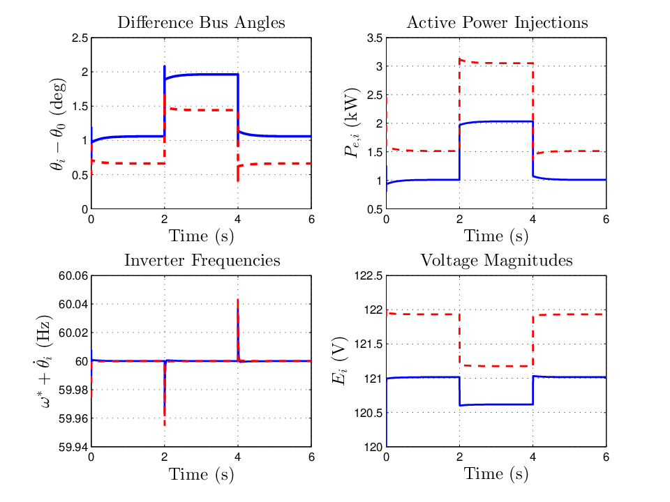
We now illustrate the performance of our proposed DAPI controller (15)–(16) and its robustness to unmodeled voltage dynamics (see Corollary 5) and lossy lines in a simulation scenario. We consider two inverters operating in parallel and supplying a variable load. The voltage magnitude at each inverter is controlled via the voltage-droop method

References

- [1] A. Arenas, A. Díaz-Guilera, J. Kurths, Y. Moreno, and C. Zhou. Synchronization in complex networks. Physics Reports, 469(3):93–153, 2008.
- [2] S. Barsali, M. Ceraolo, P. Pelacchi, and D. Poli. Control techniques of dispersed generators to improve the continuity of electricity supply. In IEEE Power Engineering Society Winter Meeting, pages 789–794, New York, NY, USA, January 2002.
- [3] N. Biggs. Algebraic potential theory on graphs. Bulletin of the London Mathematical Society, 29(6):641–683, 1997.
- [4] S. Bolognani and S. Zampieri. A distributed control strategy for reactive power compensation in smart microgrids, 2011. Available at http://arxiv.org/abs/1106.5626.
- [5] F. Bullo, J. Cortés, and S. Martínez. Distributed Control of Robotic Networks. Princeton University Press, 2009.
- [6] M. C. Chandorkar, D. M. Divan, and R. Adapa. Control of parallel connected inverters in standalone AC supply systems. IEEE Transactions on Industry Applications, 29(1):136–143, 1993.
- [7] H.-D. Chiang. Direct Methods for Stability Analysis of Electric Power Systems. Wiley, 2011.
- [8] H.-D. Chiang and C. C. Chu. Theoretical foundation of the BCU method for direct stability analysis of network-reduction power system models with small transfer conductances. IEEE Transactions on Circuits and Systems I: Fundamental Theory and Applications, 42(5):252–265, 1995.
- [9] L. O. Chua, C. A. Desoer, and E. S. Kuh. Linear and Nonlinear Circuits. McGraw-Hill, 1987.
- [10] E. A. A. Coelho, P. C. Cortizo, and P. F. D. Garcia. Small-signal stability for parallel-connected inverters in stand-alone AC supply systems. IEEE Transactions on Industry Applications, 38(2):533–542, 2002.
- [11] M. Dai, M. N. Marwali, J.-W. Jung, and A. Keyhani. Power flow control of a single distributed generation unit with nonlinear local load. In IEEE Power Systems Conference and Exposition, pages 398–403, New York, USA, October 2004.
- [12] F. Dörfler and F. Bullo. On the critical coupling for Kuramoto oscillators. SIAM Journal on Applied Dynamical Systems, 10(3):1070–1099, 2011.
- [13] F. Dörfler and F. Bullo. Kron reduction of graphs with applications to electrical networks. IEEE Transactions on Circuits and Systems I: Regular Papers, 60(1):150–163, 2013.
- [14] F. Dörfler, M. Chertkov, and F. Bullo. Synchronization in complex oscillator networks and smart grids. Proceedings of the National Academy of Sciences, 110(6):2005–2010, 2013.
- [15] E. C. Furtado, L. A. Aguirre, and L. A. B. Tôrres. UPS parallel balanced operation without explicit estimation of reactive power – a simpler scheme. IEEE Transactions on Circuits and Systems II: Express Briefs, 55(10):1061–1065, 2008.
- [16] J. M. Guerrero, L. GarciadeVicuna, J. Matas, M. Castilla, and J. Miret. Output impedance design of parallel-connected UPS inverters with wireless load-sharing control. IEEE Transactions on Industrial Electronics, 52(4):1126–1135, 2005.
- [17] J. M. Guerrero, J. C. Vasquez, J. Matas, M. Castilla, and L. G. de Vicuna. Control strategy for flexible microgrid based on parallel line-interactive UPS systems. IEEE Transactions on Industrial Electronics, 56(3):726–736, 2009.
- [18] P. Kundur. Power System Stability and Control. McGraw-Hill, 1994.
- [19] R. Lasseter and P. Piagi. Providing premium power through distributed resources. In Annual Hawaii Int. Conference on System Sciences, pages 4042–4051, Maui, HI, USA, January 2000.
- [20] Y. U. Li and C.-N. Kao. An accurate power control strategy for power-electronics-interfaced distributed generation units operating in a low-voltage multibus microgrid. IEEE Transactions on Power Electronics, 24(12):2977–2988, 2009.
- [21] J. A. P. Lopes, C. L. Moreira, and A. G. Madureira. Defining control strategies for microgrids islanded operation. IEEE Transactions on Power Systems, 21(2):916–924, 2006.
- [22] R. Majumder, A. Ghosh, G. Ledwich, and F. Zare. Power system stability and load sharing in distributed generation. In Power System Technology and IEEE Power India Conference, pages 1–6, New Delhi, India, October 2008.
- [23] M. N. Marwali, J.-W. Jung, and A. Keyhani. Stability analysis of load sharing control for distributed generation systems. IEEE Transactions on Energy Conversion, 22(3):737–745, 2007.
- [24] C. D. Meyer. Matrix Analysis and Applied Linear Algebra. SIAM, 2001.
- [25] Y. Mohamed and E. F. El-Saadany. Adaptive decentralized droop controller to preserve power sharing stability of paralleled inverters in distributed generation microgrids. IEEE Transactions on Power Electronics, 23(6):2806–2816, 2008.
- [26] R. Olfati-Saber, J. A. Fax, and R. M. Murray. Consensus and cooperation in networked multi-agent systems. Proceedings of the IEEE, 95(1):215–233, 2007.
- [27] W. Ren, R. W. Beard, and E. M. Atkins. Information consensus in multivehicle cooperative control: Collective group behavior through local interaction. IEEE Control Systems Magazine, 27(2):71–82, 2007.
- [28] S. H. Strogatz. From Kuramoto to Crawford: Exploring the onset of synchronization in populations of coupled oscillators. Physica D: Nonlinear Phenomena, 143(1):1–20, 2000.
- [29] L. A. B. Tôrres, J. P. Hespanha, and J. Moehlis. Power supplies dynamical synchronization without communication. In IEEE Power & Energy Society General Meeting, San Diego, CA, USA, July 2012. To appear.
- [30] A. Tuladhar, H. Jin, T. Unger, and K. Mauch. Parallel operation of single phase inverter modules with no control interconnections. In Applied Power Electronics Conference and Exposition, pages 94–100, Atlanta, GA, USA, February 1997.
- [31] B. W. Williams. Power Electronics: Devices, Drivers, Applications and Passive Components. McGraw-Hill, 1992.
- [32] H. Xin, Z. Qu, J. Seuss, and A. Maknouninejad. A self organizing strategy for power flow control of photovoltaic generators in a distribution network. IEEE Transactions on Power Electronics, 26(3):1462–1473, 2011.
- [33] W. Yao, M. Chen, J. Matas, J. M. Guerrero, and Z.-M. Qian. Design and analysis of the droop control method for parallel inverters considering the impact of the complex impedance on the power sharing. IEEE Transactions on Industrial Electronics, 58(2):576–588, 2011.
- [34] Q.-C. Zhong. Robust droop controller for accurate proportional load sharing among inverters operated in parallel. IEEE Transactions on Industrial Electronics, 60(4):1281–1290, 2013.
- [35] Q.-C. Zhong and T. Hornik. Control of Power Inverters in Renewable Energy and Smart Grid Integration. Wiley-IEEE Press, 2013.
Appendix A Proof of Theorem 8
Consider the closed-loop (17)–(19) arising from the DAPI controller (15)–(16). We formulate our problem in the error coordinates , and write (17)–(19) in vector notation as