A No-Arbitrage Model of Liquidity in Financial Markets involving Brownian SheetsThanks: With the collaboration of Thanh Hoang

David German Note: Claremont McKenna College Henry Schellhorn Note: Claremont Graduate University

August 24, 2026

Abstract

We consider a dynamic market model where buyers and sellers submit limit orders. If at a given moment in time, the buyer is unable to complete his entire order due to the shortage of sell orders at the required limit price, the unmatched part of the order is recorded in the order book. Subsequently these buy unmatched orders may be matched with new incoming sell orders. The resulting demand curve constitutes the sole input to our model. The clearing price is then mechanically calculated using the market clearing condition. We use a Brownian sheet to model the demand curve, and provide some theoretical assumptions under which such a model is justified.

Our main result is the proof that if there exists a unique equivalent martingale measure for the clearing price, then under some mild assumptions there is no arbitrage. We use the Ito-Wentzell formula to obtain that result, and also to characterize the dynamics of the demand curve and of the clearing price in the equivalent measure. We find that the volatility of the clearing price is (up to a stochastic factor) inversely proportional to the sum of buy and sell order flow density (evaluated at the clearing price), which confirms the intuition that volatility is inversely proportional to volume. We also demonstrate that our approach is implementable. We use real order book data and simulate option prices under a particularly simple parameterization of our model.

The no-arbitrage conditions we obtain are applicable to a wide class of models, in the same way that the Heath-Jarrow-Morton conditions apply to a wide class of interest rate models.

1 Introduction

Most liquidity models in mathematical finance abstract the trading mechanism from the characterization of prices in the resulting market. Our viewpoint is fundamentally different. In our model the equilibrium prices of the assets are completely determined by the order flow, which is viewed as an exogenous process. We model a market of assets without a specialist, where every trader submits limit orders, that is, for a buy order, the buyer specifies the maximum price, or the buy limit price, that he/she is willing to pay, and, for a sell order, the seller specifies the minimum price, or the sell limit price, at which he/she is willing to sell ¹¹ 1 There is no loss of generality in this statement. A buy market order can be specified in our model as a buy limit order with the limit price equal to infinity. Since we model assets with only positive prices, a sell market order can be specified in our model as a sell limit order with a limit price equal to zero..

If at a given moment in time, the buyer is unable to complete his entire order due to the shortage of sell orders at the required limit price, the unmatched part of the order is recorded in the order book. A symmetric outcome follows in the case of incoming sell orders. Subsequently these buy unmatched orders may be matched with new incoming sell orders. We note that many electronic exchanges, such as NYSE Arca [arc11], operate like this. Time-priority is used to break indeterminacies of a match between an incoming buyer at at the limit price superior to the ask price, i.e., the lowest limit price in the sell order book. As the result, the equilibrium of clearing price process is always defined.

Since the matching mechanism does not add any information to the economy, all information about asset prices is included in the order flow. Whether public exchanges should or should not reveal the real-time data contained in the order book is an important issue, which continues to preoccupy the financial markets community [WW02]. Our theoretical framework accommodates either viewpoint, but our empirical application is better tailored to the viewpoint that order books are public information. The current blossoming of the trading activity [Eng00], [BLT06], [Hau08], [AS08], [BRZ09] seems to confirm our viewpoint that traders are (i) interested in understanding order book information, and (ii) trade on that information.

We do not address in this paper the issue of differential information. The market microstructure literature (such as [Kyl85], and all following models) considers various models of trading involving uninformed traders, called noise traders, and one or several informed traders. One of the key results of the Kyle model is that, given the information available to the noise traders, the resulting price process is a martingale in the appropriate measure, whereas it may not be for the informed traders. As a consequence we do not believe that abstracting issues of differential information is limiting. The order books reflect all the public information. We will show (under certain conditions) that the clearing price is a martingale in the filtration corresponding to the public information, and not private information.

There are roughly two different class of models in the liquidity literature. The first class of models ([Jar92], [Jar94], [PS98b], [PS98a], [Fre98], [SW00], [BB04], [RS10]) considers the action of a large trader who can manipulate the prices in the market. There are mainly two different types of strategies a large trader can employ to that effect. The first one is to corner the market, and then squeeze the shorts. The second one is to ”front-run one’s own trades”. While some exchanges have rules to curtail the cornering of the market, the front-running seems more difficult to ban from an exchange. It is known in discrete-time trading, that, if there is no possibility of arbitrage for small traders in periods where the large investor does not trade, then there is no market manipulation strategy. In this paper, we assume that Jarrow’s conditions ([Jar94]) for the absence of the market manipulation strategy in discrete time hold. We exploit then the theoretical results from [BB04], and [KR09] to prove the absence of arbitrage in our continuous-time model, under certain conditions.

The second class of models ([ÇJP04], [ÇR07], [ÇST10], [GS11] abstracts the issues of the market manipulation away, and considers all traders as price-takers. In particular, [ÇJP04] introduced an exogenous residual supply curve against which an investor trades. The investor trades market orders, and his/her order is matched instantaneously. As a consequence of the instantaneity, it is plausible for [ÇJP04] to assume the ”price effect of an order is limited to the very moment when the order is placed in the market” (dixit [BB04]), so that that the residual supply curve at a future time is statistically independent from the order just matched. For us however, since all information is contained in the order flow, this assumption is not plausible, since it does not explain how prices can incorporate information from the arrival of new orders.

The key to our approach is to distinguish between what we call the cross orders, i.e., the orders submitted at a limit price such that they are likely to be instantaneously matched, and what we call the uncross orders, i.e., orders which will spend a positive amount of time in the order books before being either matched or cancelled. We are not aware of workable assumptions in the literature that warrant the absence of arbitrage strategy involving the uncross orders. For cross orders however the task is simpler, and our approach takes advantage of the results presented in [BB04], which assume that trading is immediate. Anecdotal evidence shows however that market manipulation strategies tend in practice to occur over short periods of time, casting doubts on the practicality of implementing market manipulation strategies with uncross orders.

In our model all the information is contained in a Brownian sheet. The Brownian sheet drives the dynamics of the demand curve. The advantage of using a Brownian sheet is that we have the same cardinality of independent sources of noise (namely, the cardinality of a real interval) as the cardinality of the set of exogenous stochastic processes. Our methodology generalizes the nonlinear partial differential equation approaches contained in the literature cited above, in the same way that the Heath-Jarrow-Morton methodology generalizes term structure models.

The main result in our article is to prove that if there exists a unique equivalent martingale measure $\mathbb{Q}$ for the clearing price, then (under some mild conditions) there is no arbitrage. We use the Ito-Wentzell formula to obtain that result, and also to characterize the dynamics of the demand curve and of the clearing price in the measure $\mathbb{Q}$ . We find that the volatility of the clearing price is (up to a stochastic factor) inversely proportional to the sum of the buy and sell order flow densities (evaluated at the clearing price), which confirms the intuition that the volatility is inversely proportional to the volume. We also demonstrate that our approach is implementable. Although we do not prove a second fundamental theorem of asset pricing, we naively use a special parameterization of our model to price options. As in the early days of the Heath-Jarrow-Morton methodology, we use only historical estimation (in our case, of the order book) to fit our model and to solve for the market price of risk. We expect that, should this paper meet with interest around practitioners, market-implied implementations will see the day. Unsurprisingly, we obtain a smile curve for the implied volatility. We note that this particular feature is not a very strong sign of the adequacy of our approach to model asset prices, as most models that came after [BS73] result in a smile curve for the implied volatility. Although limited, our results are however encouraging. They show that a fairly demanding theoretical model can be easily implemented.

The structure of the paper is as follows. In Section 2, we introduce two classes of models, one with atomistic traders only, and one with atomistic traders and a large trader. In the first one, almost by definition, the demand curve turns out to be continuous in time. In the second one, continuity (under a set of assumptions) is proved. For both models, we prove that there exist one or several martingale measures $\mathbb{Q}$ for the clearing price and that under these measures there is no arbitrage. In Section 3, we characterize the price process under the risk-neutral measure, giving the conditions under which it is unique. In Section 4, we describe our data set and the methodology we used to extract the relevant information. We also present our implementation, namely a simulation of option prices under the risk-neutral measure.

2 Model

We assume a filtered probability space ( $\Omega,\mathcal{F},\{\mathcal{F}_{t}\},\mathbb{P}$ ). We will see later what processes generate the filtration.

2.1 The Market Mechanism

A buy limit order specifies how many shares a trader wants to buy, and at what maximum price he is willing to buy them. We call this price the (buy) limit price. A buy limit order specifies how many shares a trader wants to buy, and at what maximum price he is willing to buy them. We call this price the (sell) limit price. Both buy and sell limit prices are denoted by $p$ , and should not be confused with the clearing price, which is denoted by $\pi(t)$ . The unmatched buy and sell orders are kept in order books until they are either cancelled or matched with an incoming order. An incoming order is matched with the order in the opposite side of the market which has the best price. The clearing price of the transaction is equal to the limit price of the order in the book, and not of the incoming order. Partial execution is allowed, and ties are resolved by the time-priority. Below we present an example of the matching mechanism in discrete time, that is at most one order arrives at time $t\in\{0,1,2,..\}.$

Example 2.1.

Suppose that the clearing price at time $0$ is any price $\pi(0)\in[100,120]$ . After clearing, that is, when $0<t<1$ we suppose that the order book contains the following orders

Buy Order Book
Price	Quantity
100	10

Sell Order Book
Price	Quantity
120	10
130	10

At time $t=1$ a buy order arrives with a limit price of $125, and a quantity of 15. The exchange matches it with the best sell order, i.e., the one with a sell limit price of $120. However, the execution is only partial, and the remainder of the buy order is placed in the order book at the limit price of $120, resulting in the following order book:

Buy Order Book
Price	Quantity
100	10
125	5

Sell Order Book
Price	Quantity
130	10

The clearing price at time 1 is equal to the limit price of the sell order, i.e.:

\pi(1)=120.

This example illustrates several properties of the limit order markets. First, the clearing price is always defined, and can assume any positive value ²² 2 We do not consider markets for swaps, where the prices can be negative..

Second, it is not inconceivable that an incoming order ”crosses” the order book, i.e., for the case of a buy order, that it best higher limit price than the best sell order limit price, or best ask, since the buyer does not lose a cent. Crossing the book is indeed advantageous for two reasons: first, it allows for faster execution. In our example, had the buyer submitted an order at price $130 he would have bought the complete quantity of shares (15) that he desired, rather than waiting an indeterminate amount of time until enough sell orders arrive at his limit price. Second, suppose that several buy orders are submitted at the same time. In case the demand exceeds the supply at the best ask, the buy orders with the highest limit price are executed first. Our own data analysis (see section 4) shows that few orders cross the NYSE ArcaBook [arc11]. This is consistent with the theory of optimal order book placement suggested by Rosu [Ros09].

Assumption 2.1.

Buy and sell limit prices can assume any real value between $0$ and $S$ . They are usually denoted by $p$ . Orders can be submitted to the market at any time $t\in\mathbb{R}^{+}$ .

2.2 The Brownian Sheet

We now turn our attention to the continuous-time case. Note that we do not prove convergence of a discrete-time model to our continuous-time model. We take the latter as a given, plausible model of the market. We start with a probability space $(\Omega,\mathcal{F},\mathbb{P})$ satisfying the usual conditions. The uncertainty is described by a one-dimensional Brownian sheet $W(t,s)$ , which is a continuous version of the construction (4.20) in [DPZ92] p. 100, i.e.:

W(t,s)=\sum_{j=1}\beta_{j}(t)\int\limits_{0\leq\alpha\leq s}g_{j}(\alpha)d\alpha,\text{ \ for\ }t\geq 0,0\leq s\leq S

Here $\{\beta_{j}\}$ is a family of independent real-valued standard Wiener processes, and $\{g_{j}\}$ is an orthonormal and complete basis for some Hilbert space. The variable $t$ refers to time and the variable $s$ identifies the ”factor” information necessary to model a large collection of processes identified by the variable $p$ , with $0\leq p\leq S$ . While the bound $S$ is usually taken to be equal to one in the literature, we assume instead that $S$ is a large value for ease of modeling, as will become clear later. The filtration $\{\mathcal{F}_{t}\}$ is generated by the collection of Wiener processes $\{\beta_{j}\}$ . A stochastic integral of an $\mathcal{F}_{t}$ -adapted integrand $\sigma(t,s)$ with respect to the Brownian sheet is denoted by:

I(T,S)=\int_{0}^{T}\int_{0}^{S}\sigma(t,s)W(dt,ds)

2.2.1 A Market with Atomistic Traders

Definition 2.1.

The net demand curve $Q$ is a function $[0,S]\times\mathbb{R}^{+}\times\Omega\mathbb{\rightarrow R}$ , which value $Q(p,t,\omega)$ is equal to the difference between the quantity of shares available for purchase and the quantity of shares available for sale at price $p$ and at time $t$ . For each $p$ the stochastic process $Q(.,t,.)$ is $\mathcal{F}_{t}$ -adapted. The random variables $Q(p,t,.)$ are assumed to be uniformly bounded in $p$ and $t$ almost surely.

The net demand curve represents then the information available in the (limit) order books of the exchange.

Remark 2.1.

As we will see, the process $Q$ will be assumed to be continuous in time, and we will prove that the clearing price is continuous in this model. Thus we do not need to specify in this model whether $Q$ represents the net demand just before clearing, or right after clearing, since these quantities move continuously. The same remark will not apply a priori in our model with a large trader.

Remark 2.2.

The net demand curve is decreasing in $p$ .

Definition 2.2.

The clearing price $\pi(t)$ is an $\mathcal{F}_{t}$ -adapted stochastic process which either satisfies

Q(\pi(t_{-}),t)=0,

(1)

when there is a solution to (1), or is otherwise defined by continuation, i.e., $\pi(t)$ is equal to the value of $\pi$ at the latest time $s<t$ for which there was a solution to $Q(\pi(s_{-}),s)=0$ .

When the net demand curve is continuous in time, we have of course, for any $t$ :

Q(\pi(t),t)=Q(\pi(t),t_{+}).

(2)

Definition 2.3.

A limit order submitted at time $t$ crosses the market at time $t$ if:

•

either it is a buy order with limit price $p>\pi(t_{-})$
•

or it is a sell order with limit price $p<\pi(t_{-})$

We call these orders cross orders. All the other orders are called uncross orders.

In practice it is rare that limit orders cross the market, indeed there are equilibrium models in which such orders are not rational [Ros09].

Remark 2.3.

There is a more general way to model a market. We could accumulate all of the buy order quantities with limit price higher than $p$ that enter the system (and withdraw the cancelled quantities when an order is cancelled) into a cumulative demand curve $\mathcal{D}(p,t)$ . Likewise we could accumulate all of the sell order quantities with limit price less than $p$ that enter the system (and also withdraw the cancelled quantities) into a cumulative supply curve $\mathcal{S}(p,t)$ . We call these curves ”cumulative” because we include the order quantities that are matched in them, and thus, if no order is cancelled, these curves increase in $t$ . We observe that:

Q=\mathcal{D}-\mathcal{S}

Thus, modeling only the net demand curve is reductive. While there is a (not very natural) way to extend the results of this paper to a model including both the cumulated demand and supply curves, we decided to present here only our simpler model for the following reasons. As we argued in the previous section, orders rarely ”cross”, there is a numerical instability when modeling both $\mathcal{D}$ and $\mathcal{S}$ .

Remark 2.4.

Due to Assumption 2.4, the clearing price is limited to take values between $0$ and $S$ . The frontier $\pi(t)=0$ corresponds to a bankruptcy, and the frontier $\pi(t)=S$ corresponds to a higher limit (say $S=\$1M$ ) set by the exchange to prevent excessive speculation.

Remark 2.5.

Questions of uniqueness of the clearing price will be addressed when we describe the stochastic differential equation that the clearing price (should it exist) satisfies.

The next assumption is standard. Note that by ”transaction costs” we do not mean the liquidity cost incurred, but an additional cost per transaction that the exchange would charge the traders. For instance, a buyer would pay per share a cost $\pi(t)+c$ , with $c>0$ .

Assumption 2.2.

The market is frictionless, i.e. $c=0$ .

We now develop a model for the order quantity specified in any order. Modeling a net demand curve which is twice differentiable with respect to price is clearly easier than modeling a discrete curve, and we assume it. It can occur when there is an uncountably infinite amount of traders, and traders are atomistic. We need however to rule out a degenerate case when a subset of non-zero measure of all the traders agree on the limit price, thus generating a discontinuity in the demand. This can be justified by assuming differential information amongst traders about the real value of the stock, as in the market microstructure literature. Note that the atomistic traders do not need to be noise traders for the market to be consistent. Indeed, we can (but do not need to) assume that all traders know all the information contained in the order books at all times. If they do know this information, as specified in the introduction, the clearing price does not bring any extra information as the traders can compute the clearing price by themselves at all times ³³ 3 In order to account for the delay in information processing, it would be more plausible to assume that the information available to all traders at time $t$ corresponds to $\mathcal{F}_{t-}$ and not $\mathcal{F}_{t}$ but this would complicate the model significantly, while yielding not much extra conceptual value.. Making the order book public information can be an important assumption in some settings. Indeed, our empirical studies (see Section 4) show that the order flow is tightly concentrated around the current clearing price. This confirms the obvious intuition that traders are strategic and choose their limit price based on their (slightly delayed) knowledge of the clearing price. In this paper we will fit a parametric model to the market which exploits this intuition. Our model is fairly robust when the net demand is modelled as a function of the difference in price $p-\pi(t)$ , but not robust when it is modelled (as discussed above) as a function of the limit price $p$ without a reference to the whole order book information.

Assumption 2.3.

There is a continuum of atomistic buyers and sellers who trade on the market. The resulting net demand curve $Q$ is twice differentiable in price $p$ and continuous in $t$ . We assume that

		$\displaystyle\left.\frac{\partial Q}{\partial p}\right\|_{p=0}=\left.\frac{\partial Q}{\partial p}\right\|_{p=S}=0$
		$\displaystyle\left.\frac{\partial Q}{\partial p}\right\|_{p}<0,\text{ \ \ \ for }0<p<S$

For the moment we just state the stochastic differential equation that $Q$ satisfies, assuming that the resulting net demand curve satisfies Assumption 2.3. We defer the task of showing examples where these conditions are satisfied to the next chapter, since in the next model the exact same conditions will have to apply, and it is more convenient for the reader to have a single place with the exact specification of the model. Thus

	$\displaystyle dQ(p,t)$	$\displaystyle=$	$\displaystyle\mu_{Q}(p,t)dt+\sigma_{Q}(p,t)\int_{s=0}^{S}b_{Q}(p,s,t)W(ds,dt),\text{ \ for \ }0\leq p\leq S$		(3)
	$\displaystyle Q(p,0)$	$\displaystyle=$	$\displaystyle Q_{0}(p),\text{ \ for \ }0\leq p\leq S$

The coefficients $\mu_{Q}$ , $\sigma_{Q}$ , and $b_{Q}$ are $\mathcal{F}_{t}$ -adapted. For the moment we just assume that they are such that the solution to (3) exists, is unique, and is uniformly bounded in $p$ and $t$ almost surely. Besides, for every $p$ , the process $Q(p,.)$ is a semimartingale. Also, we enforce:

\int_{s=0}^{S}b_{Q}^{2}(p,s,t)ds=1,\text{ \ for every \ }p\text{ and }t.

Definition 2.4.

A (trading) strategy $\theta=(\theta(t))$ is a semimartingale that represents a number of shares held by the investor at each point in time. If the strategy is self-financing (see e.g. [BB04] for a definition) the process $\beta^{\theta}$ representing the value of the cash account is uniquely defined.

We refer the reader to [Jar94] for a definition of market manipulation strategies in discrete time.

Definition 2.5.

For every real-valued $x$ an inverse process $P(x,t)$ satisfies

Q(P(x,t),t)=x.

(4)

The process $P(x,t)$ is undefined when (4) does not admit a solution.

Remark 2.6.

Since $Q$ is strictly monotonic in $p$ , then whenever $Q$ exists, it is also unique.

Definition 2.6 ((3.1) in [BB04]).

The asymptotic liquidation proceeds $L(\vartheta,t)$ are defined as:

L(\vartheta,t)=\int_{0}^{\vartheta}P(x,t)dx.

This definition is from [BB04] for the proceeds of a fast liquidation strategy of a large trader from $\vartheta$ to $0$ . The intuition behind this process will become more clear when we consider a market with a large trader.

Definition 2.7.

The real wealth process achieved by a self-financing trading strategy $\theta$ is given by

V^{\theta}(t)=\beta^{\theta}(t)+L(\theta(t),t)

Lemma 2.1 (Lemma 3.2 in [BB04]).

For any self-financing semimartingale strategy $\theta$ , the dynamics of the real wealth process $V^{\theta}$ are given by

		$\displaystyle V^{\theta}(t)-V^{\theta}(0_{-})$		(5)
		$\displaystyle\quad=\int_{0}^{t}L(\theta(u_{-}),du)-\frac{1}{2}\int_{0}^{t}P^{\prime}(\theta(u_{-}),u)d[\theta,\theta]_{s}^{c}-\sum_{0\leq u\leq t}\int_{\theta(u_{-})}^{\theta(u)}\{P(\theta(u),u)-P(x,u)\}dx.$

Definition 2.8.

An arbitrage (strategy) is a self-financing trading strategy $\theta$ such that $V^{\theta}(0_{-})=0$ and

	$\displaystyle\mathbb{P}(V^{\theta}(t)$	$\displaystyle>$	$\displaystyle 0)>0,$
	$\displaystyle\mathbb{P}(V^{\theta}(t)$	$\displaystyle>$	$\displaystyle 0)\geq 0.$

Theorem 2.1.

Suppose in addition to our standing assumptions that

C1) for self-financing strategies involving only cross orders, Jarrow’s [Jar94] discrete-time conditions for absence of market manipulation strategy hold,

C2) no arbitrage strategy involves uncross orders,

C3) the volatility $\sigma_{Q}(p,t)$ is bounded away from zero, uniformly in $p$ ,

C4) there is no path such that $Q(S,t)\geq 0$ or $Q(0,t)\leq 0$ .

Then

F1) there exists at least one martingale measure $\mathbb{Q}$ for $\int L(\vartheta,dt)$ ,

F2) there is no arbitrage strategy,

F3) the clearing price $\pi(t)$ is continuous,

F4) any such measure $\mathbb{Q}$ is also a martingale measure for $\pi(t)$ .

Proof.

All arguments of the proof of Theorem 2.2 can be used, replacing the (non-infinitesimal) strategy $\theta$ of the large trader by an infinitesimal strategy $\theta dp$ of an atomistic trader. Since Theorem 2.2 is more general, we will only show the proof of Theorem 2.2. ∎

A market composed only of atomistic traders is not very realistic. In the next section, we will show that under certain conditions a large trader can be added to our market, and the no-arbitrage conditions can still be obtained.

2.3 A Market with Atomistic Traders and a Large Trader

A continuous (in time) net supply curve can also arise when large traders decide to split their large orders into atomistic orders. [ÇJP04] show that this is indeed an optimal strategy in their model. The same decision turns out to be optimal in our model, under certain conditions which are elaborated in the next assumptions. We will prove this fact in Theorem 2.2, thus making our model is self-consistent.

Compared to [ÇJP04], there are two main conceptual difficulties when adding a large trader into the model. First, the trader may submit orders which are not instantaneously matched, unlike the market orders in the [ÇJP04] model. This is why we consider separately in this section the cross orders and the uncross orders. The cross orders will be matched instantaneously, and thus they behave like market orders in the [ÇJP04] model, and continuity (in time) can be proved. For uncross orders, one would need a more detailed economic model to specify in which cases it is advantageous for traders to submit a continuous (in time) order flow. Rather than going into these details, we assume that this holds true. In any event, market manipulation strategies (such as market cornering) are probably more likely to be implemented with cross orders than with uncross orders.

The second difficulty is that we have to prove that the large trader cannot manipulate the market. The conditions in [Jar94] apply when traders can submit orders at discrete time intervals. [BB04] and [KR09] show the conditions under which the discrete-time conditions extend to continuous time, and our proof of consistency of the market with a large trader will consist in part in checking that [KR09] conditions apply.

Since the continuity in time of the net demand is not assumed any more (see Remark 2.1), we need now to distinguish between the incoming orders (or the order flow) of the large trader, and the order book position.

Definition 2.9.

The net demand curves of a large (atomistic) trader $Q_{L}$ ( $Q_{A}$ ) is a function $[0,P]\times\mathbb{R}^{+}\times\Omega\mathbb{\rightarrow R}$ whose value $Q_{L}(p,t,\omega)$ ( $Q_{A}(p,t,\omega)$ ) is equal to the difference between the quantity of shares submitted for purchase and the quantity of shares submitted for sale at price $p$ at time $t$ . For each $p$ the stochastic processes $Q_{L}(.,t,,)$ and $Q_{A}(.,t,.)$ are $\mathcal{F}_{t}$ -adapted semimartingales. As before the net demand of the atomistic traders satisfies

	$\displaystyle dQ_{A}(p,t)$	$\displaystyle=$	$\displaystyle\mu_{Q_{A}}(p,t)dt+\sigma_{Q_{A}}(p,t)\int_{s=0}^{S}b_{Q_{A}}(p,s,t)W(ds,dt)\text{ \ for \ }0\leq p\leq S,$		(6)
	$\displaystyle Q_{A}(p,0)$	$\displaystyle=$	$\displaystyle Q_{A,0}(p)\text{ \ for \ }0\leq p\leq S.$

Definition 2.10.

For every real-valued $x$ the process $P_{A}(x,t)$ satisfies

Q_{A}(P_{A}(x,t),t)=x.

(7)

Definition 2.11.

The asymptotic liquidation proceeds of the large trader $L_{L}(\vartheta,t)$ are defined by

L_{L}(\vartheta,t)=\int_{0}^{\vartheta}P_{A}(x,t)dx.

Assumption 2.4.

Both $Q_{L}$ and $Q_{A}$ are twice differentiable in $p$ . Only $Q_{A}$ is assumed to be continuous in $t$ .

Remark 2.7.

The (total) net demand curve satisfies

Q=Q_{L}+Q_{A}.

Assumption 2.5.

For simplicity we assume

Q(0,t)>0.

Assumption 2.6.

For each $p\geq\pi(t)$ , the function $Q_{L}(p,t)$ is continuous in time.

Theorem 2.2.

Suppose in addition to the standing assumptions that

C1) for self-financing strategies involving only cross orders, Jarrow’s [Jar94] discrete time conditions for absence of market manipulation strategy hold,

C2) no arbitrage strategy involves uncross orders,

C3) the volatility $\sigma_{Q_{A}}(p,t)$ is bounded away from zero, uniformly in $p$ ,

C4) there is no path such that $Q(S,t)\geq 0$ or $Q(0,t)\leq 0$ .

Then

F1) there exists at least one martingale measure $\mathbb{Q}$ for $\int L_{L}(\vartheta,dt)$ ,

F2) there is no arbitrage strategy,

F3) the net demand curve $Q$ is continuous in $t$ ,

F4) the clearing price $\pi(t)$ is continuous,

F5) any such measure $\mathbb{Q}$ is also a martingale measure for $\pi(t)$ .

The full proof is presented in the Appendix. Here we show only a summary of the proof.

Summary of the Proof: We verify that the [KR09] conditions hold. Thus $\int L_{L}(\vartheta,dt)$ is a $\mathbb{Q}$ -martingale, and no market manipulation exists that involves cross orders. We prove that tame strategies ( $\theta$ continuous in $t$ ) are optimal for the large trader so that, first $Q$ is continuous in $t$ ., and, second, cross orders are traded only at the clearing price $\pi(t)$ .

∎

Remark 2.8.

Under certain conditions it is possible to extend our model to more than one large trader on the market. Following the assumptions of Theorem 2.2, the net supply curve $Q$ in a market with one large trader is indistinguishable from the net supply curve in a market with only atomistic traders. It is thus plausible that, should a second large trader arrive in the market, he would behave like the first large trader. However, there are many different ways to justify this result, and we believe that this discussion would be more appropriate in an economics journal than here.

3 Characterization of the Price Process in the Risk-Neutral Measure

In this section we characterize the price process in either one of the market models we specified earlier, since they turned out to be equivalent for our purposes.

Assumption 3.1.

To avoid repetition we assume in this section that there is no path such that $Q(S,t)\geq 0$ or $Q(0,t)\leq 0$ .

Definition 3.1.

The market price of risk $\lambda$ is a function $[0,S]\times\mathbb{R}^{+}\times\Omega\mathbb{\rightarrow R}$ . The market price of risk process $\lambda(s,.,.)$ is an $\mathcal{F}_{t}$ -adapted semimartingale for every $s\in[0,S].$ We define the $\mathbb{Q}$ -measure as a measure such that the process $W^{\mathbb{Q}}$ is a Brownian sheet, where:

W^{\mathbb{Q}}(ds,dt)=W(ds,dt)+\lambda(s,t)dt.

(8)

We can then define the clearing price process as

d\pi(t)=\sigma_{\pi}(t)\int_{s}b_{\pi}(s,t)W^{\mathbb{Q}}(ds,dt),

with

\int_{s}b_{\pi}(s,t)^{2}ds=1.

(9)

Since $Q(p,t)$ must be strictly decreasing in $p$ , we find it convenient to slightly modify the definition into:

Q(p,t)=Q(p,0)-\int_{0}^{p}q(y,t)dy,

where we define $Q(0,t)$ and $q(p,t)$ (for $0<p\leq S$ ) to be strictly positive processes with

$\displaystyle dQ(0,t)$	$\displaystyle=\mu_{Q}(0,t)dt-\sigma_{Q}(0,t)\int_{s}b_{q}(0,s,t)W(ds,dt)\quad Q(0,0)=Q_{0}(0),$	(10)
$\displaystyle dq(p,t)$	$\displaystyle=\mu_{q}(p,t)dt+\sigma_{q}(p,t)\int_{s}b_{q}(p,s,t)W(ds,dt)\quad q(p,0)=Q_{0}(p),$	(11)
	$\displaystyle\text{ \ for }0<p\leq S$
$\displaystyle q(0,t)$	$\displaystyle=0.$

Like before, the coefficients of the equations (10) and (11) are $\mathcal{F}_{t}$ -adapted. We assume that the solution to (10) and (11) exists, is unique, and is uniformly bounded in $p$ and $t$ almost surely. Also, we require that

\int_{s=0}^{S}b_{q}^{2}(p,s,t)ds=1\text{ \ for every \ }p\text{\ and \ }t.

Remark 3.1.

The process $q$ is a density of orders. By definition

	$\displaystyle q(p)dp$	$\displaystyle=$	$\displaystyle\text{quantity of shares available for purchase \ with limit price in }[p,p+dp]\text{ }$
			$\displaystyle\text{ + quantity of shares available for sale with limit price in }[p,p+dp].$

Remark 3.2.

Assuming that $Q(0,t)$ is twice-differentiable in $p$ , we must make sure that $q(p,t)$ is differentiable in $p$ , for the process $Q(p,t)$ to be twice-differentiable in $p$ . This occurs if, for instance,

dq(p,t)=\int_{s=0}^{p}(p-s)W(ds,dt).

We now define the following processes:

$\displaystyle C(\pi,t)$	$\displaystyle=$	$\displaystyle-\sigma_{\pi}(t)\left(\frac{\partial}{\partial p}\left(\sigma_{Q}(0,t)\int_{s}b_{q}(0,s,t)b_{\pi}(s,t)ds\right)+\sigma_{q}(\pi(t),t)\int_{s}b_{q}(\pi,s,t)b_{\pi}(s,t)ds\right),$
$\displaystyle b(\pi,t)$	$\displaystyle=$	$\displaystyle-\mu_{Q}(0,t)+\int_{0}^{\pi}\mu_{q}(p,t)dpdt+\frac{1}{2}\frac{\partial q}{\partial p}(\pi,t)(\sigma_{\pi}(t))^{2}-C(\pi,t),$
$\displaystyle\Sigma(\pi,s,t)$	$\displaystyle=$	$\displaystyle\int_{0}^{\pi}\sigma_{q}(p,t)b_{q}(p,s,t)ds$

Remark 3.3.

If one is not interested in modeling the correlation between orders at a different limit price, one may think that a Brownian sheet is not necessary, in the same way that the Heath-Jarrow-Morton model is often implemented with only 2 factors⁴⁴ 4 Note however that Carmona and Tehranchi [CT06] show that the Heath-Jarrow-Morton model, if there are less factors than forward rates, may result in a special type of arbitrage.. As we shall see however, the full complexity of a Brownian sheet is necessary for the market price of risk equations to have a solution.

Definition 3.2.

The market price of risk equations are:

\int_{s=0}^{P}\Sigma(\pi,s,t)\lambda(s,t)ds=b(\pi,t),\text{ \ for \ }0\leq\pi\leq P.

Theorem 3.1.

Suppose that the previous assumptions hold true. In addition, suppose that the market price of risk equations have a unique solution. Then there is no arbitrage.

Proof.

A market clears if $Q(p(t),t)=0$ , or, equivalently, if $dQ(p(t),t)=0$ . We use the Ito-Wentzell formula to compute $dQ(p(t),t)$ and set $dQ(p(t),t)=0$ .

	$\displaystyle\mu_{Q}(0,t)dt$	$\displaystyle-\int_{0+}^{\pi(t)}\mu_{q}(p,t)dpdt-\int_{0}^{\pi(t)}\sigma_{q}(p,t)\int_{s}b_{q}(p,s,t)W(ds,dt)dp$		(12)
		$\displaystyle-q(\pi(t),t)\sigma_{\pi}(t)\int_{s}b_{\pi}(s,t)W^{{}^{\mathbb{Q}}}(ds,dt)-\frac{1}{2}\frac{\partial q}{\partial p}(\pi(t),t)(\sigma_{\pi}(t))^{2}dt+C(\pi(t),t)dt=0.$

We equate the volatility terms to zero above and find

\sigma_{\pi}(t)b_{\pi}(s,t)=-\frac{\int_{0}^{\pi(t)}\sigma_{q}(p,t)b_{q}(p,s,t)dp}{q(\pi(t),t)}.

(13)

We substitute (8) in (12) and equate the drift terms to zero. This results in

	$\displaystyle\int_{s}\int_{0}^{\pi(t)}$	$\displaystyle\sigma_{q}(p,t)b_{q}(p,s,t)dp\lambda(s,t)ds=$
		$\displaystyle\quad-\mu_{Q}(0,t)+\int_{0+}^{\pi(t)}\mu_{q}(p,t)dpdt+\frac{1}{2}\frac{\partial q}{\partial p}(\pi(t),t)(\sigma_{\pi}(t))^{2}-C(\pi(t),t).$

Since the above must hold for any value of $\pi(t)$ , then the market price equations must be satisfied. Thus there exists a unique measure $\mathbb{Q}$ such that $\pi$ is a martingale. By theorems 2.1 and 2.2, there exists a non-empty set $\mathcal{Q}$ of martingale measures for $\int L(\vartheta,dt)$ . Besides, any measure $\mathbb{\tilde{Q}\in}$ $\mathcal{Q}$ must be a martingale measure for $\pi$ . Uniqueness of $\mathbb{Q}$ ensures that $\mathcal{Q=\{}\mathbb{Q\}}$ , thus $\mathbb{Q}$ is a martingale measure for $\int L(\vartheta,dt)$ . Therefore Theorems 2.1 and 2.2 imply no arbitrage. ∎

Remark 3.4.

In a numerical implementation, the market price of risk equations will be a set of $S$ linear equations with $S$ linear unknowns. Generically, like other market price of risk equations in finance, these will admit a unique solution. This was the case in all our simulations.

Remark 3.5.

Integrating (13) and using (9), we see that

\sigma_{\pi}(t)=\frac{(\int_{0}^{S}(\int_{0}^{\pi(t)}\sigma_{q}(p,t)b_{q}(p,s,t))^{2}dpds)^{1/2}}{q(\pi(t),t)}.

(14)

The denominator of (14) shows that more orders at the clearing price decrease volatility. This is to be expected. The effect of the numerator is harder to analyze, and shows that the volatility of the whole net demand curve affects the volatility of the clearing price.

Before we move to the implementation of our model, we perform an empirical analysis of the market, which will guide us in specifying a parametric model.

4 Empirical Analysis

4.1 Implementation

To the best of our knowledge, our methodology to model prices is quite original. In the same way that the HJM methodology opened the way to the development of several parametric models, we hope that this paper will result in an effort to develop models for the demand curve that are appropriate for risk management. This section only scratches the surface of that effort. Alternatively, this is what practitioners would call a ”proof of concept”, showing that the model can be implemented without too much effort. We do not make any claims about the power of the model we present hereafter, which is perhaps the simplest no-arbitrage model imaginable in our framework.

Compared to the Heath-Jarrow-Morton model for the forward rates, it is necessary in our model to know the drift of $Q(p,t)$ in the physical measure in order to simulate the price in the risk-neutral measure. In practice, there are two different methods to determine this drift: historical estimation or market implied. In the historical estimation method, one calibrates the physical drift $\mu_{Q}(0,t)$ in the model to market observables, and then solves for the market price of risk. In the market implied method, one calibrates the model to, say, a smile curve of option prices, like for other stochastic volatility models. This paper fell short of proving a second fundamental theorem of asset pricing, which would justify the implied market method. This will be a goal a subsequent paper.

In our implementation, we first use the historical estimation method to estimate the drift of $Q$ in the physical measure, and then calculate options prices by simulation, in essence assuming that the second fundamental theorem works.

4.2 A Model with Relative Prices

As explained in the introduction, and shown later, a model will be more robust if it assumes a direct dependence between the net demand curve $Q(p,t)$ and the relative prices $p-\pi(t)$ . This takes into account the fact that the investors observe the market in real-time. We are then obligated to introduce $Q(p,\pi,t)$ as the net demand curve at price $p$ when the clearing price is $\pi$ . We have then as before

$\displaystyle Q(p,\pi(t),t)$	$\displaystyle=$	$\displaystyle Q(0,\pi(t),t)-\int_{0}^{\pi(t)}q(p,\pi(t),t)dp,$	(15)
$\displaystyle dq(p,\pi(t),t)$	$\displaystyle=$	$\displaystyle\mu_{q}(p,\pi(t),t)dt+\sigma_{q}(p,\pi(t),t)\int_{s}b_{q}(p,\pi(t),s,t)W(ds,dt),$
$\displaystyle dQ(0,\pi(t),t)$	$\displaystyle=$	$\displaystyle\mu_{Q}(0,\pi(t),t)dt-\sigma_{q}(0,\pi(t),t)\int_{s}b_{q}(0,\pi(t),s,t)W(ds,dt).$

Let

F(\pi,t)=Q(0,\pi,t)-\int\limits_{0}^{\pi}q(p,\pi,t)dp.

Then

F_{\pi}(\pi,t)=\frac{\partial Q(p,\pi,t)}{\partial\pi}-q(\pi,\pi,t)-\int\limits_{0}^{\pi}\frac{\partial}{\partial\pi}q(p,\pi,t)dp

and

F_{\pi\pi}(\pi,t)=\frac{\partial^{2}Q(0,\pi,t)}{\partial\pi^{2}}-q_{p}(\pi,\pi,t)-q_{\pi}(\pi,\pi,t)-\frac{\partial}{\partial\pi}q(\pi,\pi,t)-\int\limits_{0}^{\pi}\frac{\partial^{2}}{\partial\pi^{2}}q(p,\pi,t)dp.

We define

H(s,\pi,t)=-\int\limits_{p=0}^{\pi}\sigma_{q}(p,\pi,t)b_{q}(p,\pi,s,t)dp.

Hence

\frac{\partial}{\partial\pi}H(s,\pi,t)=-\int\limits_{p=0}^{\pi}\frac{\partial\sigma_{q}}{\partial\pi}[\sigma_{q}(p,\pi,t)b_{q}(p,\pi(t),s,t)]dp-\sigma_{q}(\pi,\pi,t)b_{q}(\pi,\pi,s,t).

Therefore the Ito-Wentzell’s formula takes the form

	$\displaystyle dQ(\pi(t),t)$	$\displaystyle=$	$\displaystyle\mu_{Q}(0,\pi(t),t)-\int\limits_{p=0}^{\pi(t)}\mu_{q}(p,\pi(t),t)dt-\sigma_{q}(p,\pi(t),t)\left(\int_{s}b_{q}(p,\pi(t),s,t)W(ds,dt)\right)dp$
			$\displaystyle+F_{\pi}(\pi(t),t)d\pi(t)+\frac{1}{2}F_{\pi\pi}(\pi(t),t)(d\pi)^{2}+C(\pi(t),t)dt,$

where

C(\pi(t),t)=\sigma_{\pi}(t)\int\frac{\partial}{\partial\pi}H(s,\pi(t),t)ds.

Market clears if $dQ(\pi(t),t)=0$ . Equating the volatilities results in

\sigma_{\pi}(t)b_{\pi}(s,t)=\frac{\int_{0}^{\pi(t)}\sigma_{q}(p,\pi(t),t)b_{q}(p,\pi(t),s,t)dp}{F_{\pi}(\pi(t),t)}.

Apart from the denominator, this is the same equation as (13). We now define

b(\pi,t)=\int_{0}^{\pi}\mu_{q}(p,\pi,t)dp-\mu_{Q}(0,\pi,t)-\frac{1}{2}F_{\pi\pi}(\pi(t),t)\sigma_{\pi}^{2}(t)-C(\pi(t),t).

(16)

Finally, the market price of risk equations can be expressed as

\int_{s}\left(\int_{0}^{\pi}\sigma_{q}(p,\pi,t)b_{q}(p,\pi,s,t)dp\right)\lambda(s,t)ds=b(\pi,t).

(17)

4.3 A Parametric Implementation with Relative Prices

We discretize our model in 3 dimensions: time $t$ , limit price $p$ and factor $s$ . For the market price of risk equations to have a unique solution the number of price buckets where orders are assigned should be equal to $S$ , namely the number of factors. We let $\Delta p$ be the size of a price bucket.

We define the relative price $k$ as

k\equiv p-\pi,

and the relative net demand $\tilde{Q}(k,\pi,t)$ as

\tilde{Q}(k,\pi,t)=Q(p,\pi,t).

We simplify the model above (as expressed in (15)), and assume that the order flow depends only on the relative price $k$ , i.e., $\tilde{Q}(k,\pi,t)=$ $\tilde{Q}(k,t)$ . Now assume without loss of generality that $S$ is even, and define $K=S/2$ . We model the relative net demand curve as

\tilde{Q}(k,t)=\tilde{Q}(-K,t)+\sum_{l=-K+1}^{k}\tilde{q}(l,t).

In our model, the logarithm of the order flow quantities follow Ornstein-Uhlenbeck processes. This ensures the stationarity as well as the positivity of the order flow quantities. In other terms

$\displaystyle d\log\tilde{Q}(0,t)$	$\displaystyle=-a_{Q}(0)(\log\tilde{Q}(0,t)-\log\hat{Q}(0))dt+\sigma_{Q}^{rel}(0)\sum_{j=-K+1}^{K}b_{q}(k,j)\sqrt{\Delta p}dW_{j}(t)$	(18)
$\displaystyle d\log\tilde{q}(k,t)$	$\displaystyle=-a_{q}(k)(\log\tilde{q}(k,t)-\log\hat{q}(k))dt+\sigma_{q}^{rel}(k)\sum_{j=-K+1}^{K}b_{q}(k,j)\sqrt{\Delta p}dW_{j}(t)\text{, with }$	(19)
	$\displaystyle k=-K+1..K$

It is thus necessary to estimate the parameters $a_{q}(k)\geq 0$ , $a_{Q}(0)\geq 0$ , $\sigma_{q}^{rel}(k)$ and $b_{q}(k,j)$ , as well as the initial values. We notice that our model is not twice differentiable in $p$ , however, for our parameter values, it does not behave significantly differently from a smoothed version of that model.

4.3.1 Results

Data:

We collected high frequency data from NYSE ArcaBook [arc11] for General Electric Company (GE) on April 1^st, 2011. GE limit order is characterized by six intrinsic quantities: (1) message type: e.g. “A”: add new order,“M”: modify order, “D”: delete order; (2) trading type: e.g. “B”: buy limit order or “S”: sell limit order; (3) time: recorded when a new event occurs, e.g. add new order, modify order or delete order; (4) ID: a unique identifier of each limit order; (5) price in dollars; and (6) size in number of shares.

We selected data during the trading time from 9:30 AM to 4:00 PM EST. Before doing any analysis, we removed obvious errors in the data, e.g. abnormal prices of USD 122 or USD 0.01. We managed to keep track of approximately 90% of the original limit orders. For the cancellation of limit orders, we assumed that if the amount of time was less than or equal 2 minutes when the “delete” message occurred after the “modify” message of the same order, this order was cancelled.

Let $p_{\text{min}}$ be the minimum price of USD 20.00 and $p_{\text{max}}$ be the maximum price of USD 20.62 during the trading day. We partitioned the price space into 5 cents bins

	$\displaystyle p_{\text{min}}=20.00$	$\displaystyle=$	$\displaystyle p_{-K}<p_{-K+1}<\dots<p_{K-1}<p_{K}=p_{\text{max}}=20.62$
	$\displaystyle p_{K+1}-p_{K}$	$\displaystyle=$	$\displaystyle\Delta p~(5~\text{cent}).$

Likewise, we partitioned the time into:

t_{i+1}-t_{i}=\Delta t~(1~\text{minute})

Clearing Prices $\pi(t)$ :

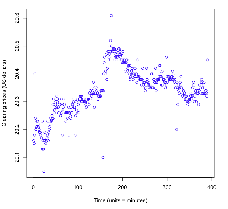
By dividing the time period from 9:30 AM to 4:00 PM EST into one-minute time intervals, we obtained 390 one-minute time intervals (6.5 trading hours * 60 minutes).

Table 1: Statistical Summary for

\pi(t)

Summary	Output	Summary	Output
nobs	390	SE Mean	0.004174
NAs	0	LCL Mean	20.3294
Minimum	20.05	UCL Mean	20.3458
Maximum	20.61	Variance	0.006795
1. Quartile	20.29	Stdev	0.082435
3. Quartile	20.39	Skewness	-0.289841
Mean	20.338	Kurtosis	0.277282
Median	20.340	Sum	7931.68

Jarque-Bera Test:

We implemented the Jarque-Bera test to check the null hypothesis H₀ that the clearing prices $\pi(t)$ are normally distributed (while H₁ is the hypothesis that $\pi(t)$ are not normally distributed). The Jarque-Bera test used both skewness and kurtosis simultaneously to check the normality of the selected data. The Jarque-Bera test statistic was calculated as

\text{JB}=(S^{*})^{2}+(K^{*})^{2},

where

S^{*}=\sqrt{\frac{T}{6}}\ \widehat{S}\left(\pi(t)\right)\sim N(0,1)\qquad\text{ and }\qquad K^{*}=\sqrt{\frac{T}{24}}\left(\widehat{K}\left(\pi(t)\right)-3\right)\sim N(0,1).

The Jarque-Bera test yielded the p-value of 3.161%, which is below the default significance level of 5%. Thus, we rejected the null hypothesis $H_{0}$ that the clearing prices $\pi(t)$ are normally distributed. However, with the p-value of 3.161%, the distribution of $\pi(t)$ is rather close to a normal distribution, which is also shown in Figure 1.

Refer to caption — Figure 1: The density of clearing prices $\pi(t)$

Evolution of $\pi(t)$ :

From the result of linear regression, we obtained the constant value of the drift of clearing prices $\pi(t)$ . Thererfore, we have

	$\displaystyle d\pi(t)$	$\displaystyle=$	$\displaystyle cdt+\sigma_{\pi}(t)\int_{s}b_{\pi}(s,t)W(ds,dt),$
			$\displaystyle\qquad\qquad\qquad\qquad\text{where: }c=0.000374764.$

Buy Limit Orders:

Let us recall the definition of $\tilde{Q}$

	$\displaystyle\log\tilde{Q}(-K,i\Delta t)$	$\displaystyle=$	$\displaystyle\log\left(\sum\text{number of buy orders}*\text{buy order quantity arriving before}\ i\Delta t\right),$
			$\displaystyle\qquad\qquad\text{where }\Delta t=1\!\text{ minute}.$

We tested the data of $\log\tilde{Q}(i\Delta t)$ for one-minute time interval with the autocorrelation and partial autocorrelation functions. The ACF and PACF figures showed (see Figure 3) that the data of $\log\tilde{Q}(i\Delta t)$ for one-minute time interval were fitted in the autoregressive AR(1) model.

Results:

We conducted the estimation of our model (18), (19) over the data set described above. The opening clearing price on that day was

\pi(0)=20.16.

Using $K=7$ and $\Delta p=0.05$ , the speed of mean-reversion was obtained from the autoregressive AR(1) model. For the relative net demand curve, we observed the following initial value and relative hourly volatility:

	$\displaystyle\tilde{Q}(-K,0)$	$\displaystyle=$	$\displaystyle 1.02705\times 10^{11},$
	$\displaystyle\sigma_{Q}^{rel}(-K)$	$\displaystyle=$	$\displaystyle 0.01976.$

For the relative net demand curve density the values are reported in the following table

$k$	$q(k,0)$ [in 10¹¹]	$\sigma_{q}^{rel}(k)$ – hourly	$a(k)$
-6	0.95314	0.04883	0.11903
-5	1.41994	0.04655	0.29142
-4	2.35893	0.01706	0.25250
-3	0.82541	0.04423	0.36708
-2	0.14050	0.04877	0.36752
-1	4.13487	0.03744	0.29380
0	0.21397	0.00461	0.21991
1	9.95599	0.00379	0.25219
2	4.61052	0.03496	0.36316
3	3.51037	0.00653	0.15248
4	2.42507	0.01224	0.19830
5	0.14219	0.00036	0.34405
6	2.70257	0.00969	0.13387

Table 2: Statistics for the relative net demand curve density

We then simulated the lognormal model (18), (19) using $N=100$ scenarios and approximated the value of a call option:

C(\psi)=\frac{1}{N}\sum_{\omega=1}^{N}\max(\pi(T,\omega)-\psi,0),

where $\psi$ is a strike price for an expiration $T$ =0.02, that is, roughly equal to one week. We then calculated the implied volatility of the call for each strike price, that is, the value $\sigma^{imp}($ Strike $)$ such that the Black-Scholes value of the call option equals $C(K)$ , and this for each $K$ . The resulting function $\sigma^{imp}($ Strike $)$ as a function of the strike price ( the smile curve) is reported in Figure 4 below.

As expected, the smile is fairly pronounced, which is an indicator that our model engenders fat tails in the risk-neutral distribution of $\pi(T)$ .

5 Appendix

Lemma 5.1.

Let

$\displaystyle\mu_{P}(x,t)$	$\displaystyle=$	$\displaystyle-\frac{\mu_{Q_{A}}(P_{A}(x,t),t)+\frac{1}{2}\frac{\partial^{2}Q_{A}}{\partial p^{2}}(P_{A}(x,t),t)\sigma_{P}^{2}(x,t)+\frac{\partial\sigma_{Q_{A}}}{\partial p}(P_{A}(x,t),t)\sigma_{p}(t)}{\frac{\partial Q}{\partial p}(P_{A}(x,t),t)}$
$\displaystyle\sigma_{P}(x,t)$	$\displaystyle=$	$\displaystyle\frac{\sigma_{Q_{A}}(P_{A}(x,t),t)}{\frac{\partial Q_{A}}{\partial p}(P_{A}(x,t),t)}$
$\displaystyle b_{P}(x,s,t)$	$\displaystyle=$	$\displaystyle b_{Q_{A}}(P_{A}(x,t),t),s,t)$

Then $P_{A}$ is a semimartingale and satisfies

dP_{A}(x,t)=\mu_{P}(x,t)dt+\sigma_{P}(x,t)\int\limits_{0}^{S}b_{P}(x,s,t)W(ds,dt)

(20)

Proof.

By definition:

Q_{A}(P_{A}(x,t),t)=x

(21)

We suppose that (20) holds and apply the Ito-Wentzell formula (see e.g., [Kry09]) to both sides of (21) yields:

		$\displaystyle\mu_{Q_{A}}(P_{A}(x,t),t)+\frac{\partial Q_{A}}{\partial p}(P_{A}(x,t),t)\mu_{P}(x,t)$
		$\displaystyle\qquad\qquad\qquad\ +\frac{1}{2}\frac{\partial^{2}Q_{A}}{\partial p^{2}}(P_{A}(x,t),t)\sigma_{P}^{2}(x,t)+\frac{\partial\sigma_{Q_{A}}}{\partial p}(P_{A}(x,t),t)\sigma_{P}(x,t)=0,$
		$\displaystyle\sigma_{Q_{A}}(P_{A}(x,t),t)b_{Q_{A}}(P_{A}(x,t),s,t)+\frac{\partial Q_{A}}{\partial p}(P_{A}(x,t),t)\sigma_{P}(x,t)b_{P}(x,s,t)=0$

∎

Proof of Theorem 2.2

For fact (F1), we first check assumptions (RF) in [KR09]:

(i) Since $L_{L}(\vartheta,t)$ is a semimartingale, it is a strong integrator.

(ii) We calculate

\frac{\partial^{2}L_{L}(\vartheta,t)}{\partial\vartheta^{2}}=\frac{\partial}{\partial x}P_{A}(\vartheta,t)=\frac{1}{\frac{\partial Q^{A}}{\partial p}(P_{A}(\vartheta,t))}.

Since $Q^{A}$ is strictly decreasing and twice differentiable in $p$ , then its inverse $P_{A}$ is differentiable in $\vartheta$ and $\frac{\partial^{2}L_{L}(\vartheta,t)}{\partial\vartheta^{2}}$ is continuous in $\vartheta$ .

(iii) Since $\frac{\partial L_{L}(\vartheta,t)}{\partial\vartheta}=P_{A}(\vartheta,t)$ is a semimartingale, it is a strong integrator.

(iv) By the Lemma 5.1 the quadratic variation of $L_{L}(\vartheta,.)$ is equal to

[L_{L}(\vartheta,.),L_{L}(\vartheta,.)]_{t}=\int_{0}^{t}\int_{0}^{\vartheta}\left(\frac{\sigma_{Q}(P_{A}(x,t),t)}{\frac{\partial Q}{\partial p}(P_{A}(x,t),t)}\right)^{2}dt.

This is clearly strictly increasing if $\sigma_{Q}(P_{A}(x,t),t)$ is uniformly bounded away from zero, which holds if $\sigma_{Q}(p,t)$ is uniformly bounded away from zero on $0<p<S$ .

Thus assumptions (RF) are satisfied. We now define the market price of risk as

\lambda^{(x)}(s,t)=\frac{\mu_{P}(x,t)}{\sigma_{P}(x,t)}.

Since $\mu_{P}(x,t)$ is bounded and $\sigma_{P}(x,t)$ is non-zero, then the assumption (UB) in [KR09] is satisfied. To check the assumption (UI) we refer the reader to [KR09] for the definition of $\lambda_{t}^{(n)}$ and $[M^{(n)},M^{(n)}]$ . Since both $Q_{A}$ and $Q_{L}$ are uniformly bounded, the integrand $\lambda_{t}^{(n)}$ is bounded. By the same reason, and because of the continuity (in time) of $Q_{A}$ , the quadratic variation $[M^{(n)},M^{(n)}]$ is bounded. Thus (UI) holds, and Theorem 3.5 in [KR09] holds, proving Fact (F2).

Fact (F2) follows directly from the comments after Theorem 3.5 in [KR09], which we quote here, while adjusting for our notation and formulae numbering:

“Consider now again the dynamics (5) of the real wealth process, and let $\theta$ be such that $\int L_{L}(\theta,ds)$ is bounded from below (the transaction costs term in (5) can be avoided by the large trader by using only tame strategies). An arbitrage opportunity is an admissible strategy such that we have for the associated real wealth process $V^{\theta}$ that $V^{\theta}(0)\leq 0,\ V^{\theta}(T)\geq 0$ $\mathbb{P}$ -a.s., and $\mathbb{P}(V^{\theta}(T)>0)>0$ . By Theorem 3.5 in [KR09], there exists a probability measure $\mathbb{Q}$ such that $\int L_{L}(\theta,ds)$ is a $\mathbb{Q}$ -local martingale, hence a supermartingale. It follows now from the dynamics (5) of the real wealth process that $\mathbb{E}_{\mathbb{Q}}[V^{\theta}(T)]\leq V^{\theta}(0)$ which, as $\mathbb{Q}$ is equivalent to $\mathbb{P}$ , excludes arbitrage opportunities for the large trader.“

We can now prove the continuity of $\pi(t)$ . Since by assumption uncross orders result in $Q_{L}$ being continuous in time, a discontinuity can arise only from cross orders. Suppose that the large trader is a net buyer (for a sell strategy the argument is identical), i.e, that there is an $\varepsilon>0$ such that for all $0\leq\delta\leq\varepsilon$

\theta(t+\delta)-\theta(t)\geq 0.

Suppose that

\displaystyle\pi(t)-\pi(t_{-})\geq\epsilon_{2}>0.

(22)

Then, since $\partial Q_{A}/\partial p>0$ and $Q_{A}$ is assumed to be twice differentiable

-Q_{A}(\pi(t),t)+Q_{A}(\pi(t_{-}),t)\geq\epsilon_{3}>0.

By continuity in time of $Q_{A}$

-Q_{A}(\pi(t),t_{+})+Q_{A}(\pi(t_{-}),t)\geq\epsilon_{4}>0.

An examination of terms in Lemma 3.3 in [BB04] shows that discontinuous strategies are suboptimal for the trader, i.e.

\displaystyle\theta(t_{+})-\theta(t)=0.

(23)

By definition

\theta(t_{+})-\theta(t)=-Q_{A}(\pi(t),t_{+})+Q_{A}(\pi(t_{-}),t).

However, this shows, that (22) contradicts (23). Thus $\pi$ is continuous, proving fact (F4), and

\displaystyle Q_{L}(\pi(t),t)-Q_{L}(\pi(t_{-}),t)=0.

(24)

By definition also

	$\displaystyle\theta(t_{+})-\theta(t)$	$\displaystyle=Q_{L}(\pi(t),t_{+})-Q_{L}(\pi(t_{-}),t)$		(25)
		$\displaystyle=Q_{L}(\pi(t),t_{+})-Q_{L}(\pi(t),t)+Q_{L}(\pi(t),t)-Q_{L}(\pi(t_{-}),t).$

Combining (23), (24) and (25) we obtain that

Q_{L}(\pi(t),t_{+})-Q_{L}(\pi(t),t)=0.

This shows that the net demand curve is continuous in $t$ , thus proving fact (F3).

Finally, we build the curve:

Q=Q_{L}+Q_{A}.

Suppose that a new atomistic trader comes to the market. She will trade at a price $\pi(t)$ and will have liquidity costs:

\int\limits_{0}^{t}L(\theta(u),du)=\int_{0}^{t}\theta(u)d\pi(u).

Since $\int\limits_{0}^{t}L(\theta(u),du)$ is a $\mathbb{Q}$ -martingale, therefore $\pi$ is a $\mathbb{Q}$ -martingale, too.

∎

References

[arc11] NYSE ArcaBook FTP Client Specification, version 1.5a. www.nyxdata.com/doc/37716, June 2011.
[AS08] Marco Avellaneda and Sasha Stoikov. High-frequency trading in a limit order book. Quantitative Finance, 8(3):217–224, April 2008.
[BB04] Peter Bank and Dietmar Baum. Hedging and portfolio optimization in financial markets with a large trader. Math. Finance, 14(1):1–18, 2004.
[BLT06] Tim Bollerslev, Julia Litvinova, and George Tauchen. Leverage and volatility feedback effects in high-frequency data. Journal of Financial Econometrics, 4(3):353–384, 2006.
[BRZ09] Federico Bandi, Jeffrey Russell, and Yinghua Zhu. Using high-frequency data in dynamic portfolio choice. Working paper, 2009.
[BS73] Fischer Black and Myron Scholes. The pricing of options and corporate liabilities. The Journal of Political Economy, 81(3):637–654, 1973.
[ÇJP04] Umut Çetin, Robert A. Jarrow, and Philip Protter. Liquidity risk and arbitrage pricing theory. Finance and Stochastics, 8(3):311–341, 2004.
[ÇR07] Umut Çetin and Chris Rogers. Modeling liquidity effects in discrete time. Mathematical Finance, 17:15–29, 2007.
[ÇST10] Umut Çetin, H. Mete Soner, and Nizar Touzi. Option hedging for small investors under liquidity costs. Finance and Stochastics, 14(3):317–341, 2010.
[CT06] René Carmona and Michael Tehranchi. Interest Rate Models: and Infinite Dimensional Stochastic Analysis Perspective. Springer-Verlag, 2006.
[DPZ92] Guiseppe Da Prato and Jerzy Zabczyk. Stochastic Equations in Infinite Dimensions. Cambridge University Press, 1992.
[Eng00] Robert Engle. The econometrics of ultra-high-frequency data. Econometrica, 68(1):1–23, January 2000.
[Fre98] Rüdiger Frey. Perfect option hedging for a large trader. Finance and Stochastics, 2:115–141, 1998.
[GS11] Selim Gökay and H. Mete Soner. Hedging in an illiquid binomial market. Preprint, 2011.
[Hau08] Nikolaus Hautsch. Capturing common components in high-frequency financial time series: A multivariate stochastic multiplicative error model. Journal of Economic Dynamics and Control, 32(12):3978–4015, December 2008.
[Jar92] Robert Jarrow. Market manipulation, bubbles, corners and short squeezes. Journal of Financial and Quantitative Analysis, 27:311–336, 1992.
[Jar94] Robert Jarrow. Derivative securities markets, market manipulation and option pricing theory. Journal of Financial and Quantitative Analysis, 29:241–261, 1994.
[KR09] Jan Kallsen and Thorsten Rheinländer. Financial markets with a large trader: an approach via carmona and nualart integration. Unpublished, 2009.
[Kry09] Nikolai Krylov. On the Ito-Wentzell formula for distribution-valued processes and related topics. arXiv:0904.2752v2, 2009.
[Kyl85] Albert S. Kyle. Continuous auctions and insider trading. Econometrica, 53:1315–1335, 1985.
[PS98a] George Papanicolaou and Ronnie Sircar. General Black-Scholes models accounting for increased market volatility from hedging strategies. Applied Mathematical Finance, 5:45–82, 1998.
[PS98b] Eckhard Platen and Martin Schweizer. On feedback effects from hedging derivatives. Math. Finance, 8(1):67–84, 1998.
[Ros09] Ioanid Rosu. A dynamic model of the limit order book. Review of Financial Studies, 22:4601–4641, 2009.
[RS10] Chris Rogers and Surbjeet Singh. The cost of illiquidity and its effects on hedging. Mathematical Finance, 20(4):597–615, October 2010.
[SW00] Philipp J. Schönbucher and Paul Wilmott. The feedback effect of hedging in illiquid markets. SIAM Journal on Applied Mathematics, 61(1):232–272 (electronic), 2000.
[WW02] S. Wiswanathan and James Wang. Market architecture: limit-order books versus dealership markets. Journal of Financial Markets, 5(2):127–167, April 2002.

A No-Arbitrage Model of Liquidity in Financial Markets involving Brownian SheetsThanks: With the collaboration of Thanh Hoang

Abstract

1 Introduction

2 Model

2.1 The Market Mechanism

Example 2.1.

Assumption 2.1.

2.2 The Brownian Sheet

2.2.1 A Market with Atomistic Traders

Definition 2.1.

Remark 2.1.

Remark 2.2.

Definition 2.2.

Definition 2.3.

Remark 2.3.

Remark 2.4.

Remark 2.5.

Assumption 2.2.

Assumption 2.3.

Definition 2.4.

Definition 2.5.

Remark 2.6.

Definition 2.6 ((3.1) in [BB04]).

Definition 2.7.

Lemma 2.1 (Lemma 3.2 in [BB04]).

Definition 2.8.

Theorem 2.1.

Proof.

2.3 A Market with Atomistic Traders and a Large Trader

Definition 2.9.

Definition 2.10.

Definition 2.11.

Assumption 2.4.

Remark 2.7.

Assumption 2.5.

Assumption 2.6.

Theorem 2.2.

Remark 2.8.

3 Characterization of the Price Process in the Risk-Neutral Measure

Assumption 3.1.

Definition 3.1.

Remark 3.1.

Remark 3.2.

Remark 3.3.

Definition 3.2.

Theorem 3.1.

Proof.

Remark 3.4.

Remark 3.5.

4 Empirical Analysis

4.1 Implementation

4.2 A Model with Relative Prices

4.3 A Parametric Implementation with Relative Prices

4.3.1 Results

Data:

Clearing Prices π⁡(t)\pi(t):

Jarque-Bera Test:

Evolution of π⁡(t)\pi(t):

Buy Limit Orders:

Results:

5 Appendix

Lemma 5.1.

Proof.

References

Clearing Prices $\pi(t)$ :

Evolution of $\pi(t)$ :