Disrupting Primordial Planet Signatures: The Close Encounter of Two Single-Planet Exosystems in the Galactic Disc

Disrupting Primordial Planet Signatures: The Close Encounter of Two Single-Planet Exosystems in the Galactic Disc–23XXXX

Dimitri Veras ^†^†thanks: E-mail:veras@ast.cam.ac.uk Affiliation: Institute of Astronomy, University of Cambridge, Madingley Road, Cambridge CB3 0HA Nickolas Moeckel ^†^†thanks: E-mail:nickolas1@gmail.com Affiliation: Institute of Astronomy, University of Cambridge, Madingley Road, Cambridge CB3 0HA

Accepted 2012 June 20. Received 2012 June 4; in original form 2012 May 8

Abstract

During their main sequence lifetimes, the majority of all Galactic Disc field stars must endure at least one stellar intruder passing within a few hundred AU. Mounting observations of planet-star separations near or beyond this distance suggest that these close encounters may fundamentally shape currently-observed orbital architectures and hence obscure primordial orbital features. We consider the commonly-occurring fast close encounters of two single-planet systems in the Galactic Disc, and investigate the resulting change in the planetary eccentricity and semimajor axis. We derive explicit 4-body analytical limits for these variations and present numerical cross-sections which can be applied to localized regions of the Galaxy. We find that each wide-orbit planet has a few percent chance of escape and an eccentricity that will typically change by at least $0.1$ due to these encounters. The orbital properties established at formation of millions of tight-orbit Milky Way exoplanets are likely to be disrupted.

Keywords:

planets and satellites: dynamical evolution and stability – planet-star interactions – stars: kinematics and dynamics – Galaxy: kinematics and dynamics – Galaxy: structure – celestial mechanics

1 Introduction

After leaving their birth clusters, most stars undertake a potentially harrowing multi-Gyr journey through the Galactic Disc. The stars are continuously perturbed by global Galactic phenomena and are periodically nudged by individual stellar encounters. Occasionally, an encounter is close enough to cause major disruption to any planets orbiting in the approaching systems. The currently observed exoplanet population may be shaped in part by these encounters.

1.1 Typical Closest Encounter Distances

Using simple arguments (Binney & Tremaine, 2008, e.g. from Pg. 3 of), one can crudely estimate an upper bound for the typical encounter distance, $r_{enc}$ , over a main sequence lifetime. If $n$ denotes the space density of stars in the Galactic Disc, and $v_{\rm ran}$ is the random velocity of stars, then $r_{enc}\approx(4\pi nv_{\rm ran}t_{\rm MS})^{-1/2}$ , where $t_{\rm MS}$ is the main sequence lifetime. This estimate is conservatively large because gravitational focusing is not included. We can estimate $t_{MS}$ through simulations from the SSE stellar evolution code (Hurley et al., 2000). Doing so yields Fig. 1, which plots the closest encounter main sequence distance as a function of progenitor mass from $1{\rm M}_{\odot}-2{\rm M}_{\odot}$ , which represents a common range of exoplanet host masses. The majority of stars drawn from a standard stellar initial mass function (Parravano et al., 2011, see e.g.) will have masses under 1 ${\rm M}_{\odot}$ , further suggesting that the typical encounter separations in Fig. 1 represent overestimates. The solid and dashed lines represent Solar and very low (1/200th of Solar) metallicities, respectively. The metallicity of a star helps dictate its main sequence lifetime, and hence the expected close encounter distance. The plot partially illustrates that differences in the metallicity of stars have little (indirect) effect on the close encounter distance.

The figure demonstrates that the majority of all stars will suffer a close encounter of just a few hundred AU for a reasonable range of $n$ and $v_{\rm ran}$ values. Even in sparse environments, like the Solar neighborhood (with $n\approx 0.1$ pc^-3), Sun-like stars will approach one another at least once within a few hundred AU. This estimate corroborates the rough estimate of $500$ AU given by Zakamska & Tremaine (2004), who consider only a 5 Gyr encounter timescale.

Refer to caption — Figure 1: Upper bound estimates for typical main-sequence closest encounter distances, $r_{enc}$ , between exosystems in the field of the Galactic Disc. Solar metallicity stars and very low metallicity stars are represented by solid and dashed lines, respectively. The random velocity of stars is $v_{\rm ran}$ and the space density of stars is $n$ . Fiducial values of $n$ ( $0.6{\rm pc}^{-3}$ ) and $v_{\rm ran}$ ( $50{\rm km/s}$ ) are represented by the black curves. Because the majority of Galactic Disc stars are less massive than $1{\rm M}_{\odot}$ , they will have $r_{enc}$ values less than hundreds of AU.

1.2 Stellar Encounter Orientations with Respect to Galactic Centre

Given that close encounters within hundreds of AU will typically occur, we can now attempt to characterize the orientations of the collisions with respect to the Galactic Centre. As outlined by Quillen et al. (2011), the distribution of velocities in the Galactic Disc is affected by a multitude of factors. Potential perturbers include Galactic Lindblad resonances (Yuan & Kuo, 1997; Lépine et al., 2011, e.g.), stellar streams from past mergers and interactions with satellite subhaloes (Bekki & Freeman, 2003; Gómez et al., 2010, e.g.), and transient spiral density waves (De Simone et al., 2004, e.g.). Stellar velocities may also be highly dependent on the phase and pattern speed of the Milky Way’s spiral arms (Antoja et al., 2011), suggesting drastic differences in the velocity distribution in different regions. These factors might help explain why the velocity components of the stars in the Solar neighborhood are neither isotropic nor Gaussian (Binney et al., 2000; Nakajima et al., 2010). Generally, the orbits of Disc stars are modulated vertically and epicyclically (Binney & Tremaine, 2008, e.g. pgs. 164-166,), and may undergo significant radial migration (Schoenrich, 2011, e.g.). Further, the amplitude of the epicyclic and vertical oscillations are of the same order of magnitude (Binney & Tremaine, 2008, e.g., Pg. 18,), and are orders of magnitude longer than then the physical radii of the stars themselves. Therefore, we should expect that stars suffer close encounters with each other at random orientations with respect to the Galactic Centre.

1.3 Planetary Orbit Orientations with Respect to the Galactic Disc

Now we assess whether the planes of the planetary orbits should have a preferential orientation to the Galactic Disc. The severe misalignment of the Solar System’s invariable plane with the Galactic plane at $\approx 60^{\circ}$ (Huang & Wade, 1966; Duncan et al., 1987) foreshadows the likely answer. Observations constrain the distribution of exoplanetary orbital planes poorly because most extrasolar planets have been discovered by the Doppler radial velocity technique, which alone does not provide any information about line-of-sight inclinations. Similarly, the stellar rotational axis orientation – which is suggestive of planetary orbit orientation – of the vast majority of non-exoplanet host stars is unknown. However, in cases where this information has been obtained, Abt (2001) and Howe & Clarke (2009) find that the these axes are orientated randomly. For exoplanet-host stars that harbour transiting planets, we do have line-of-sight inclination information. According to the Exoplanet Data Explorer¹¹ 1 See the Exoplanet Data Explorer at http://exoplanets.org/, as of 15 January, 2012, there are 141 transiting exoplanets. At most, the orbital plane of any of these planets is misaligned with our line-of-sight by $\approx 13.4^{\circ}$ . However, the median misalignment angle is just $\approx 2.79^{\circ}$ and the standard deviation is $\approx 2.73^{\circ}$ .

Therefore, effectively we observe transiting planets edge-on, and the locations of these planets on the sky might suggest a relation between the Galactic plane and planetary orbital planes. In Fig. 2, we plot the declination versus right ascension of the host stars of these 141 transiting planets from this database. In order to help assuage the strong observational bias in the plot, the plot markers are colored and shaped according to the planet names, which are often indicative of the program or collaboration who first discovered the planet. For example, the planets with names containing “Kepler” or “KOI” (Kepler Object of Interest) are all clustered in the same region on the plot. This is due to the the fixed field the Kepler space mission is observing. The plot definitively illustrates that observed planetary orbital planes are known to encompass a wide range of orientations with respect to the Galactic Disc.

These considerations lead us to treat close encounters between two planetary systems in arbitrary directions with orbital planes that are arbitrarily aligned with each other. However, we must sensibly restrict the vast phase space of these encounters. We do so first by reviewing some published literature related to this topic.

1.4 Extending Previous Scattering Studies

The three-body problem which includes a star-planet pair experiencing a perturbation from an intruder star has been the subject of several studies, and is well-characterized in many regions of phase space. Most studies, however, treat these interactions in the context of cluster encounters (Heggie & Rasio, 1996; Davies & Sigurdsson, 2001; Fregeau et al., 2006; Spurzem et al., 2009), which typically have a higher $n$ , smaller $v_{\rm ran}$ , and much shorter lifetime (tens of Myr) than in the field. An exception is Zakamska & Tremaine (2004), who do consider perturbations in the field from a stellar intruder, but on a multi-planet system. They treat the perturbation as a superposition of three-body interactions, neglecting the contribution to the potential from the planets. Also, they treat the velocity vector of the intruder and the orbital plane as coplanar. Among their several useful results are i) about $10\%$ of all stars experience close encounters within 200 AU, ii) planetary eccentricities may be excited up to $0.1$ in the field, and iii) the extent of the excitation is strongly dependent on system size and phase.

Here, we provide a multi-tiered extension to that work. First, we consider the potential of all four bodies in the close encounter of two one-planet systems, as most Milky Way stars are now thought to have planets (Cassan et al., 2012). Previous studies of the 4-body problem often consider the more general case of the interaction of two stellar binaries (Mikkola, 1984; Hut, 1993; Bacon et al., 1996; Heggie, 2000; Giersz & Spurzem, 2003; Fregeau et al., 2004; Pfahl & Muterspaugh, 2006; Sweatman, 2007) or a planet-less intruder perturbing a multi-planet exosystem (Malmberg et al., 2011; Boley et al., 2012). However, none of these studies consider the close encounter of two single-planet systems.

Second, because field encounters are fast, we develop an analytical method based on impulses that can determine the change in orbital parameters without resorting to numerical simulations. We consider two extremes in phase for our analysis, although the method can in principle be generalized to arbitrary phases, and even arbitrary numbers of planets.

Third, we do perform numerical simulations, here specifically for the purpose of obtaining normalized cross sections. These quantities then enable one to determine the overall rate of encounters and eccentricity excitations over a main sequence lifetime in localized patches of the Milky Way. As already argued earlier, we consider encounters of all mutual orientations, independent of their locations with respect to the Galactic Centre.

Table 1: Variables Used in this Paper

Variable	Explanation
$a_{h}$	Hyperbolic semimajor axis for a star
$a_{k0}^{(*)}$	Initial semimajor axis for planet $k$ in the far ( $=f$ ) and close ( $=c$ ) cases
$a_{kf}^{(*)}$	Final semimajor axis for planet $k$ in the far ( $=f$ ) and close ( $=c$ ) cases
$a_{\chi}^{(*)}$	Contribution to Planet #2’s semimajor axis variation due to Planet #1 alone in the far ( $=f$ ) and close ( $=c$ ) cases
$\alpha$	Number of planetary orbital periods to numerically integrate before the close encounter
$b$	Impact parameter of both stars
$b_{{\rm eje}}^{(f)}$	far case impact parameter value at which a planet escapes
$b_{{\rm eje,1}}^{(c)}$	Maximum close case impact parameter value separating planetary escape from boundedness
$b_{{\rm eje,2}}^{(c)}$	Middle close case impact parameter value separating planetary escape from boundedness
$b_{{\rm eje,3}}^{(c)}$	Minimum close case impact parameter value separating planetary escape from boundedness
$b_{\rm max}$	Maximum impact parameter used in the numerical simulations
$b_{\rm min}$	Impact parameter which causes a planet-planet collision
$b_{p1p2}$	Impact parameter of both planets
$b_{p1s2}$	Impact parameter of Planet #1 and Star #2
$b_{s1p2}$	Impact parameter of Star #1 and Planet #2
$b_{{\rm stat,<}}^{(c)}$	close case lower impact parameter value at which there is no net perturbation on the planets
$b_{{\rm stat,>}}^{(c)}$	close case upper impact parameter value at which there is no net perturbation on the planets
$\beta$	Factor by which $(a_{10}+a_{20})$ is multiplied to obtain $q$ for the numerical simulations
$\gamma$	Fraction of the innermost planetary orbit used as a numerical integration timestep bound
$\delta$	Dimensionless planet/star mass ratio for each system when both are physically equivalent
$\delta_{k}$	Dimensionless planet/star mass ratio for system $k$
$e_{\rm ext,max}^{(c)}$	close case local eccentricity maximum, for $(b_{{\rm stat,>}}^{(c)})<b$
$e_{\rm ext,min}^{(c)}$	close case local eccentricity minimum, for $b_{{\rm eje,1}}^{(c)}<b<b_{{\rm eje,2}}^{(c)}$
$e_{h}$	Hyperbolic eccentricity of a star
$e_{kf}^{(*)}$	Final eccentricity for planet $k$ in the far ( $=f$ ) and close ( $=c$ ) cases
$e_{\chi}^{(*)}$	Contribution to Planet #2’s eccentricity variation due to Planet #1 alone in the far ( $=f$ ) and close ( $=c$ ) cases
$E_{h}$	Hyperbolic anomaly of a star
$\epsilon$	Dimensionless ratio equal to $a_{10}/a_{20}$
$\eta$	Dimensionless ratio equal to $V_{\infty}/V_{\rm crit}$
$M_{pk}$	Mass of planet $k$
$M_{sk}$	Mass of star $k$
$M_{\rm tot}$	Total mass of the 4-body system
$\mu$	Sum of both stellar masses, times the Gravitational Constant
$n$	Space density of stars
$N$	Number of experiments
$\mathcal{N}$	Number of times over a main sequence lifetime that $\left\|\Delta e_{1}\right\|>\Upsilon$ occurs
$q$	Pericenter of the star-star hyperbolic orbit
$r_{\rm enc}$	Typical closest encounter distance for two stars in the Galactic Disc
$r_{\rm start}$	Separation used to initialize numerical integrations
${\rm RAND}$	Low-discrepancy quasi-random Niederreiter number between 0 and 1
$\sigma$	Cross section
$\sigma_{\rm norm}$	Normalized cross section
$t_{\rm enc}$	Timescale of close encounter between both planetary systems
$t_{\rm integrate}$	Numerical integration timescale
$t_{\rm MS}$	Main Sequence lifetime
$T_{k}$	Orbital period of planet $k$ about star $k$
$\Upsilon$	Given extent of an eccentricity perturbation
$v_{\rm ran}$	Random stellar velocity
$V_{\infty}$	Velocity of Star #1 with respect to Star #2 at an infinite separation
$V_{{\rm circ},k}$	Circular velocity of planet $k$ about star $k$
$V_{{\rm circ},k0}$	Circular velocity of planet $k$ about star $k$ assuming $M_{pk}=0$
$V_{{\rm circ},0}$	Circular velocity of either planet for equal planetary masses and semimajor axes
$V_{\rm crit}$	Velocity at which the total energy of the 4-body system equals zero
$V_{\rm peri}$	Pericenter velocity of the star-star hyperbolic orbit
$\|\Delta\vec{V}_{\bot}\|$	Magnitude of the velocity kick perpendicular to the direction of motion

1.5 Plan for Paper

We outline some of the key quantities in the hyperbolic 4-body problem in Section 2 before our analytical (Section 3 and the Appendix) and numerical (Section 4) explorations. Of particular note are the two specific orientations we model without numerical integrations (Sections 3.2.3 and 3.2.4) and the eccentricity excitation frequencies arising from our numerical integrations (Section 4.3). In Section 5, we interpret the results. Section 6 discusses related topics, and Section 7 provides a short conclusion.

1.5.1 Variables used

Table 1 delineates the variables applied throughout this paper. The subscript $k$ takes the values “1” and “2” and is used to describe the planet and star belonging to the different planetary systems taking part in the encounter. Primed and double-primed values are explained in the text where necessary.

2 4-body Problem Setup

Consider a planet with mass $M_{p1}$ orbiting a Galactic Disc star with mass $M_{s1}$ , and an independently evolving planet with mass $M_{p2}$ orbiting a different Disc star with mass $M_{s2}$ . Initially, assume the distance between the systems (denoted “1” and “2”) is infinity. Each planetary orbit is described by the planet’s semimajor axis, $a_{k}$ , and eccentricity, $e_{k}$ , where $k=1$ or $2$ depending on the planet. At $t=0$ , the orbital parameters are denoted by an additional subscript,“ $0$ ”.

As argued in Section 1, the systems may approach each other at any orientation, and the relative orientation of the planetary orbital planes is also unconstrained. Now consider the plane in which the stars approach each other, and fix the reference frame on $M_{s2}$ . System #1 will approach System #2 such that $M_{s1}$ will be traveling at a velocity $V_{\infty}$ with an impact parameter $b$ . Because $V_{\infty}>0$ the stars will approach each other on approximate hyperbolic orbits, approximate because of the presence of the planets. Denote the reduced mass of the 2-body hyperbolic system as $\mu\equiv G\left(M_{s1}+M_{s2}\right)$ . We treat values of $V_{\infty}$ , $b$ and $\mu$ , as well as all four individual masses and $a_{k0}$ , for $k=1,2$ , as given, known quantities throughout the paper. Further, $e_{k0}=0$ always.

2.1 Key Orbital Parameters

The total energy of the system is equal to $V_{\infty}^{2}/2=-\mu/2a_{h}$ , where $a_{h}$ is the (negative) hyperbolic semimajor axis. Hence

a_{h}=-\frac{\mu}{V_{\infty}^{2}}.

(1)

The total angular momentum of the system is equal to $bV_{\infty}$ , which can be related to the hyperbolic eccentricity, $e_{h}>1$ , such that

e_{h}^{2}=1+\frac{b^{2}V_{\infty}^{4}}{\mu^{2}}.

(2)

The pericenter, $q>0$ , of the star-star hyperbolic orbit is

q\equiv|a_{h}|\left(e_{h}-1\right)=\frac{\mu}{V_{\infty}^{2}}\left[\sqrt{1+\frac{b^{2}V_{\infty}^{4}}{\mu^{2}}}-1\right].

(3)

2.2 Velocity Comparisons

The total energy of a 2-body system with a nonzero relative velocity is positive. The critical velocity of the four body system, $V_{\rm crit}$ , for which the total system energy is zero and ionization is possible is (Fregeau et al., 2004):

V_{\rm crit}\equiv\sqrt{\frac{GM_{\rm tot}}{\left(M_{s1}+M_{p1}\right)\left(M_{s2}+M_{p2}\right)}\left(\frac{M_{s1}M_{p1}}{a_{10}}+\frac{M_{s2}M_{p2}}{a_{20}}\right)}

(4)

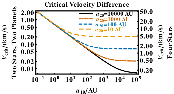
where $M_{\rm tot}=M_{s1}+M_{p1}+M_{s2}+M_{p2}$ . We plot typical values of $V_{\rm crit}$ in Fig. 3, showing that $V_{\rm crit}$ is nearly 23 times lower for two ${\rm M}_{\rm J}$ planets and two ${\rm M}_{\odot}$ stars than for four ${\rm M}_{\odot}$ stars, where ${\rm M}_{\rm J}$ is the mass of Jupiter. Hence, comparison of typical stellar velocities in the Galactic Disc ( $\approx 10$ km/s - $100$ km/s) implies that one-planet systems are moving too fast to ionize all four bodies through encounters regardless of the values of $a_{10}$ and $a_{20}$ .

Now we can compare the circular velocity of a planet with respect to its parent star, $V_{{\rm circ},k}$ , to typical values of $V_{\infty}$ . We have

V_{{\rm circ},k}=29.79\frac{\rm km}{\rm s}\sqrt{\left(\frac{M_{sk}+M_{pk}}{{\rm M}_{\odot}}\right)\left(\frac{1{\rm AU}}{a_{k0}}\right)}

(5)

Therefore, for wide orbit planets and typical Disc velocities, $V_{\infty}\gg V_{{\rm circ},k}$ . However, for planets on tight orbits, the velocities are comparable. Further, we denote $V_{{\rm circ},k0}$ as the circular velocity of planet $k$ when $M_{pk}=0$ (such that $V_{{\rm circ},k}\approx V_{{\rm circ},k0}$ ).

The fastest velocity achieved in a hyperbolic orbit is at the pericenter of that orbit. The pericenter velocity $V_{\rm peri}$ , is related to $V_{\infty}$ through

V_{\rm peri}=\sqrt{\frac{\mu}{\left|a_{h}\right|}\left[\frac{e_{h}+1}{e_{h}-1}\right]}=V_{\infty}\left[\frac{\sqrt{1+\frac{b^{2}V_{\infty}^{4}}{\mu^{2}}}+1}{\sqrt{1+\frac{b^{2}V_{\infty}^{4}}{\mu^{2}}}-1}\right]^{\frac{1}{2}}

(6)

which is always greater than $V_{\infty}$ and becomes infinite as $b\rightarrow 0$ . $V_{\infty}$ represents the minimum velocity of the orbit.

3 Impulse Analytics

Although we must resort to numerical simulations to fully explore the 4-body problem consisting of two planet-star systems, here we investigate how this cases of this problem may be solved analytically in the impulse regime. As suggested by Eq. (5), perturbations on wide orbit planets due to passing planetary systems may be treated in the impulse approximation. Zakamska & Tremaine (2004) claim that this assumption holds for their planetless intruder if the stellar perturber is fast and if the planetary period is much longer than the characteristic timescale of the encounter, $t_{\rm enc}\approx b/V_{\rm peri}$ . This condition is analogous here to

\frac{T_{k^{\prime\prime}}}{t_{\rm enc}}\approx 2\pi\frac{a_{k^{\prime\prime}}}{b}\frac{V_{\rm peri}}{V_{{\rm circ},k^{\prime\prime}}}\gg 1,

(7)

where $k^{\prime\prime}$ indicates the planet with the smaller orbital period. As demonstrated by Eq. (7), the impulse approximation is well-suited for wide orbits due to the resulting low value of $V_{{\rm circ},k^{\prime\prime}}$ . In the impulse regime, the planets do not progress in their orbits around their parent stars during the encounter (i.e., the mean anomaly is approximated as stationary).

The impulse approximation allows us to isolate and estimate analytically the planets’ mutual perturbations during the encounter. For simplicity, let us treat both planets on circular orbits. By symmetry, in the impulse approximation the only net perturbation is perpendicular to the velocity vector of the perturber. For ease of reference to Zakamska & Tremaine (2004), we also take both planetary systems to be coplanar with each other and with the perturber’s velocity vector. We will be estimating the perturbations on Planet #2. By symmetry, the perturbations on Planet #1 will yield the same change in orbital parameters.

3.1 General Case

3.1.1 Total Perturbations on the Passing Star

First, let us estimate the perturbations on Star #2 due to Star #1. Pg. 422 of Binney & Tremaine (1987) shows that the imparted velocity kick is

|\Delta\vec{V}_{\bot}|_{s1s2}=\frac{2bV_{\infty}^{3}}{\mu}e_{h}^{-2}.

(8)

Planet #1 will also kick Star #2. The effective impact parameter between Planet #1 and Star #2, $b_{p1s2}$ , will depend on the planet’s position during the encounter. We have,

|\Delta\vec{V}_{\bot}|_{p1s2}=\frac{2M_{p1}b_{p1s2}V_{\infty}^{3}}{G\left(M_{p1}+M_{s2}\right)^{2}}\left(1+\frac{b_{p1s2}^{2}V_{\infty}^{4}}{G^{2}\left(M_{p1}+M_{s2}\right)^{2}}\right)^{-1}.

(9)

3.1.2 Total Perturbations on the Passing Planet

Similarly to the impulse imparted on Star #2 by Planet #1, the impulse imparted by Star #1 on Planet #2 is:

|\Delta\vec{V}_{\bot}|_{s1p2}=\frac{2b_{s1p2}V_{\infty}^{3}}{G\left(M_{s1}+M_{p2}\right)}\left(1+\frac{b_{s1p2}^{2}V_{\infty}^{4}}{G^{2}\left(M_{s1}+M_{p2}\right)^{2}}\right)^{-1}.

(10)

The impulse on Planet #2 from Planet #1 is:

|\Delta\vec{V}_{\bot}|_{p1p2}=\frac{2b_{p1p2}V_{\infty}^{3}}{G\left(M_{p1}+M_{p2}\right)}\left(1+\frac{b_{p1p2}^{2}V_{\infty}^{4}}{G^{2}\left(M_{p1}+M_{p2}\right)^{2}}\right)^{-1}.

(11)

3.1.3 Net Perturbations on the Passing Planet

Therefore, Planet #2 experiences a net velocity kick relative to its parent star of

	$\displaystyle\|\Delta\vec{V}_{\bot}\|_{p2}$	$\displaystyle=$	$\displaystyle\|\Delta\vec{V}_{\bot}\|_{s1s2}+\|\Delta\vec{V}_{\bot}\|_{p1s2}$		(12)
		$\displaystyle-$	$\displaystyle\left(\|\Delta\vec{V}_{\bot}\|_{s1p2}+\|\Delta\vec{V}_{\bot}\|_{p1p2}\right)$		(12)

Equipped with Eqs. (8)-(12), we can insert these velocity kicks into the formalism of Jackson & Wyatt (2012) [see their Eqs. 1-2].²² 2 The assumption under which these equations are derived is that the impulse is instantaneous, which is equivalent to our Eq. (7). in order to determine the resulting variation in $a_{2}$ and $e_{2}$ . Let us denote the post-encounter values of $a_{2}$ and $e_{2}$ as $a_{2f}$ and $e_{2f}$ (recall $e_{20}=0$ ). Then

	$\displaystyle\frac{a_{20}}{a_{2f}}$	$\displaystyle=$	$\displaystyle 1-\left(\frac{\|\Delta\vec{V}_{\bot}\|_{p2}}{V_{{\rm circ},2}}\right)^{2},$		(13)
	$\displaystyle e_{2f}$	$\displaystyle=$	$\displaystyle\left\|\frac{\|\Delta\vec{V}_{\bot}\|_{p2}}{V_{{\rm circ},2}}\right\|.$		(14)

3.2 Specific Example

We wish to relate $a_{2f}$ and $e_{2f}$ to $b$ , $V_{\infty}$ and $M_{s1}$ , $M_{s2}$ , $M_{p1}$ , and $M_{p2}$ in an analytically tractable manner. Thus, we will focus on two specific cases of interest, as illustrated in Fig. 4. In the first case, which we denote by far, both planets are the furthest possible distance from each other as the systems pass each other; both stars are in-between the planets. Here, the value of $b$ may be any value from $0$ to $\infty$ . In the second case, which we denote by close, the direction of the vectors from each star to its child planet are pointing towards each other. Here, a value of $b$ that we denote $b_{\rm min}$ will cause both planets to collide. For $b<b_{\rm min}$ , the orbits will overlap. Figure 4 shows a cartoon of the encounters at pericenter for different cases.

We have derived analytical formulae for the critical points of the motion, asymptotic limits, and the individual contribution to the perturbations from the planets alone. All these formulae are presented and explained in the Appendix in order to help retain the focus of the reader here. In this section, we provide just the most important results.

3.2.1 Analytic Simplification

In order to obtain compact, understandable formulae, for the remainder of Section 3, we assume $a_{10}=a_{20}$ , $M_{p1}=M_{p2}$ and $M_{s1}=M_{s2}$ such that both systems are equivalent except for their labels. Define $\delta\equiv M_{p2}/M_{s2}$ and $V_{{\rm circ},0}$ as the circular velocity of either planet assuming the planet mass is zero. In other specific cases of interest, these assumptions may be lifted and the more general results rederived in a similar manner as below.

3.2.2 Fiducial Sample

In order to provide tangible numbers that accompany the analytics and resulting plots, we concurrently consider fiducial values of $M_{s2}={\rm M}_{\odot}$ , $M_{p2}={\rm M}_{\rm J}$ , $a_{20}=1000$ AU and $V_{\infty}=30{\rm km\ s}^{-1}\approx 1000V_{\rm crit}$ unless otherwise indicated³³ 3 Our choice of fiducial semimajor axis helps us demonstrate all of the regimes of interest for realistic close encounter distances (Fig. 1) and known exoplanet separations (Goldman et al., 2010; Kuzuhara et al., 2011; Luhman et al., 2011, e.g.).. These values give $V_{{\rm circ},2}\approx 1.3{\rm km\ s}^{-1}$ such that the impulse approximation is valid as long as $b\ll 1.45\times 10^{5}$ AU (Eq. 7).

3.2.3 The far Case

Even though the planets are at opposition to each other in the far case, planetary ejection will occur when the stars have a close-enough encounter, when $b\leq b_{{\rm eje}}^{(f)}$ . Alternatively, for $b>b_{{\rm eje}}^{(f)}$ , the orbital parameter evolution is

	$\displaystyle e_{2f}^{(f)}$	$\displaystyle\approx$	$\displaystyle\left[\frac{2\left(2a_{20}+b\right)}{a_{20}+b}\right]\left[\frac{\sqrt{\frac{GM_{s1}a_{20}}{b^{2}}}}{V_{\infty}}\right],$		(15)
	$\displaystyle a_{2f}^{(f)}$	$\displaystyle=$	$\displaystyle\frac{a_{20}}{1-e_{2f}^{{(f)}^{2}}}.$		(16)

Note that $e_{2f}^{(f)}\rightarrow 0$ and $a_{2f}^{(f)}\rightarrow a_{20}$ as $b\rightarrow\infty$ , as expected. Also, $a_{2f}^{(f)}$ cannot decrease due to the close encounter.

Equations (15)-(16) show that as long as the planetary mass is neligible compared to the stellar mass, the planetary contribution is also negligible everywhere in the far case parameter space. Nevertheless, we quantify this contribution in the Appendix. Note that $e_{2f}^{(f)}\rightarrow 0$ and $a_{2f}^{(f)}\rightarrow a_{20}$ as $b\rightarrow\infty$ , as expected. Also, $a_{2f}^{(f)}$ cannot decrease due to the close encounter.

Figure 5 illustrates these properties. Depending on $V_{\infty}$ , Planet #2 will be ejected when $b$ is within a few tens or hundreds of AU; $b_{{\rm eje}}^{(f)}$ is marked on the upper axis of the left panel for the slowest $V_{\infty}$ . Planets which remain bound after surviving a passing star at $b\approx 500$ AU expand their orbits by tens to hundreds of AU and stretch their orbits through eccentricity increases of at least $0.1$ .

3.2.4 The close Case

Now let us consider the opposite limit, where the position vectors from each star to their orbiting planet point towards each other. The resulting orbital parameter evolution is a more complicated function of $b$ .

In particular, there are two separate ranges of $b$ in which a planet will escape: i) $0<b<b_{{\rm eje,3}}^{(c)}$ , when both stars are in between both planets and the stars are close to each other, and ii) $b_{{\rm eje,2}}^{(c)}<b<b_{{\rm eje,1}}^{(c)}$ , when one star nearly collides with one planet. Further, there is one region, $(b_{{\rm stat,<}}^{(c)})<b<(b_{{\rm stat,>}}^{(c)})$ , where the planet-planet interaction becomes important. Additionally, there are two local extrema: i) in between the escape regions, the perturbations are minimized at $e_{\rm ext,min}^{(c)}$ , and ii) for $b$ well beyond $b_{\rm min}$ , the perturbations are maximized at $e_{\rm ext,max}^{(c)}$ .

All of the physical features mentioned above and illustrated in both Figs. 6 and 22 (which can be used as guides for the location of the critical points) can be reproduced with a compact analytical form for $e_{2f}^{(c)}$ as a function of impact parameter. We remind the reader that this quantity, among several others, are derived in the Appendix:

e_{2f}^{(c)}\approx\left|2\left(\frac{a_{20}}{b}\right)\left(\frac{V_{{\rm circ},0}}{V_{\infty}}\right)\frac{8G^{2}M_{s1}^{2}+Z_{4}+Z_{5}}{Z_{6}Z_{7}}\right|

(17)

such that

$\displaystyle Z_{4}$	$\displaystyle=$	$\displaystyle 2GM_{s1}V_{\infty}^{2}\left(6a_{20}-b\left(3-2\delta\right)\right)$	(18)
$\displaystyle Z_{5}$	$\displaystyle=$	$\displaystyle V_{\infty}^{4}\left(4a_{20}^{2}+b^{2}\left(1-2\delta\right)-2ba_{20}\left(2-\delta\right)\right)$	(19)
$\displaystyle Z_{6}$	$\displaystyle=$	$\displaystyle 2GM_{s1}+V_{\infty}^{2}\left(a_{20}-b\right)$	(20)
$\displaystyle Z_{7}$	$\displaystyle=$	$\displaystyle 2GM_{s1}+V_{\infty}^{2}\left(2a_{20}-b\right)$	(21)

where $a_{2f}^{(c)}$ is derived from $e_{2f}^{(c)}$ in the usual way (Eq. 16).

3.3 Consequences

The analytics show that a planet’s eccentricity can be raised to any value due to a realistic close encounter. Even in the limiting case where both planets are furthest from each other during the encounter, if the stars endure a close enough approach, then the planets will be ejected. In the other extreme, measurable eccentricity excitation can occur over a wide, realistic range of impact parameters. When a star crosses in between another star and planet, the eccentricity excitation is at least a tenth, but is likely many tenths. When any two bodies narrowly miss each other, planetary escape may occur. However, there are locations at which this net perturbation is zero; this range of locations increases along with planetary mass.

This analytic exploration helps us to gauge expectations for the outcomes of numerical simulations, and perhaps more importantly, provides an explanation for some of the trends seen in the outputs of our numerical simulations. We describe these simulations in the following section.

4 Numerical Cross Sections

We now calculate cross sections of various encounter outcomes via numerical scattering experiments. Cross sections of this type, introduced in stellar dynamical research by Hut & Bahcall (1983), represent the effective surface area for some outcome of a scattering event between involving stellar or planetary systems. Coupled with a velocity distribution and density of systems, the cross section yields a total outcome frequency. By suitably setting up random stellar encounters and performing many experiments, the probabilistic outcome of these potentially chaotic encounters can be obtained.

Here, we are interested in the frequency of planetary systems whose planets have eccentricities that are perturbed by a particular amount, $\Upsilon$ . The cross section is a function of $\Upsilon$ , $\epsilon\equiv a_{10}/a_{20}$ , and $\eta\equiv V_{\infty}/V_{\rm crit}$ such that one example is:

\sigma(\left|\Delta e_{1}\right|>\Upsilon,\epsilon,\eta)=\pi b_{\rm max}^{2}\frac{N(\left|\Delta e_{1}\right|>\Upsilon,\epsilon,\eta)}{N_{\rm total}}

(22)

where $N_{\rm total}$ represents the total number of experiments and $N(\left|\Delta e_{1}\right|>\Upsilon,\epsilon,\eta)$ represents the number of experiments with a given $\epsilon$ and $\eta$ that yield $\left|\Delta e_{1}\right|>\Upsilon$ . One may compute errors in $\sigma(\left|\Delta e_{1}\right|>\Upsilon,\epsilon,\eta)$ by using Gaussian counting statistics (Hut & Bahcall, 1983). Doing so gives error bars which are equal to the RHS of Eq. (22) divided by $\sqrt{N(\left|\Delta e_{1}\right|>\Upsilon,\epsilon,\eta)}$ . In order to create a scale-free cross section – for wider applications – $\sigma$ can be normalized as:

	$\displaystyle\sigma_{\rm norm}(\left\|\Delta e_{1}\right\|>\Upsilon,\epsilon,\eta)$	$\displaystyle=$	$\displaystyle\frac{\sigma(\left\|\Delta e_{1}\right\|>\Upsilon,\epsilon,\eta)}{\pi\left(a_{10}+a_{20}\right)^{2}}$		(23)
		$\displaystyle=$	$\displaystyle\frac{\sigma(\left\|\Delta e_{1}\right\|>\Upsilon,\epsilon,\eta)}{\pi a_{10}^{2}}\left(\frac{\epsilon}{1+\epsilon}\right)^{2}$		(23)

Our goal is to compute values of both $\sigma_{\rm norm}(\left|\Delta e_{1}\right|>\Upsilon,\epsilon,\eta)$ and $\sigma_{\rm norm}(\left|\Delta e_{2}\right|>\Upsilon,\epsilon,\eta)$ for different values of $\Upsilon$ , $\epsilon$ and $\eta$ . Doing so requires a careful numerical setup.

4.1 Numerical Simulation Setup

First, we must set up initial conditions such that the initial separation of the stars is finite, and then select this finite separation. We also must chose a sufficiently representative range of $b$ small enough to not be computationally prohibitive but large enough to encompass all the regimes in, for example, Fig. 6. Finally, we must choose values of $V_{\infty}$ that encompass a wide range of possible physical values.

4.1.1 Characterizing Finite Separations

Strictly, our numerical simulations cannot treat infinite distances. Therefore, we must propagate forward the 2-body star-star hyperbolic solution until the mutual distance between the stars, $r(t)$ , reaches a specified distance $r(t=t_{\rm start})\equiv|r_{\rm start}|$ . At this separation, the initial conditions for the numerical simulations are established. For any finite $|r_{\rm start}|$ , the components of the stars’ velocity both parallel and perpendicular to the impact parameter segment will be different than their initial values at an infinite mutual separation. Denote the position and velocity components parallel to $b$ by $x$ and $\dot{x}$ , and the perpendicular components by $y$ and $\dot{y}$ . Given values of $\mu,V_{\infty},b,$ and $|r_{\rm start}|$ of the relative orbit, we seek to derive $x_{\rm start}$ , $y_{\rm start}$ , $\dot{x}_{\rm start}$ and $\dot{y}_{\rm start}$ .

Denote the hyperbolic anomaly as $E_{h}$ . Then we adopt the same definition of $r$ as in Pg. 45 of Taff (1985) and Pg. 85 of Roy (2005) such that

\cosh{E_{h}}=\frac{1+\frac{r_{\rm start}}{a_{h}}}{e_{h}}.

(24)

Note that by this convention, $r_{\rm start}$ is negative. Through geometry, we have:

	$\displaystyle x_{\rm start}$	$\displaystyle=$	$\displaystyle a_{h}\left(e_{h}-\cosh{E_{h}}\right),$		(25)
	$\displaystyle y_{\rm start}$	$\displaystyle=$	$\displaystyle a_{h}\sqrt{e_{h}^{2}-1}\sqrt{\cosh^{2}{E_{h}}-1}.$		(26)

Differentiating these gives

	$\displaystyle\dot{x}_{\rm start}$	$\displaystyle=$	$\displaystyle-a_{h}\sqrt{\cosh^{2}{E_{h}}-1}\frac{dE_{h}}{dt},$		(27)
	$\displaystyle\dot{y}_{\rm start}$	$\displaystyle=$	$\displaystyle a_{h}\sqrt{e_{h}^{2}-1}\cosh{E_{h}}\frac{dE_{h}}{dt}$		(28)

yielding a total velocity of

\frac{dr_{\rm start}}{dt}=\pm a_{h}\frac{dE_{h}}{dt}\sqrt{e_{h}^{2}\cosh^{2}{E_{h}}-1}=\sqrt{\mu\left(\frac{2}{r_{\rm start}}-\frac{1}{a_{h}}\right)}

(29)

where the RHS is due to the properties of a two-body hyperbolic orbit. Thus,

\frac{dE_{h}}{dt}=\frac{\pm\sqrt{\mu\left(\frac{2}{r_{\rm start}}-\frac{1}{a_{h}}\right)}}{a_{h}\sqrt{e_{h}^{2}\cosh^{2}{E_{h}}-1}},

(30)

where the signs indicate the two possible velocity vectors along the orbit. Because we model the systems approaching one another, we adopt the upper sign. Subsequently, we can insert Eq. (30) into Eqs. (27) and (28) and use Eqs. (1), (2), (24) and (30) to express the starting Cartesian elements in terms of given parameters:

$\displaystyle x_{\rm start}$	$\displaystyle=$	$\displaystyle-\frac{b^{2}V_{\infty}^{2}+r_{\rm start}\mu}{\sqrt{b^{2}V_{\infty}^{4}+\mu^{2}}},$	(31)
$\displaystyle y_{\rm start}$	$\displaystyle=$	$\displaystyle-bV_{\infty}\sqrt{\frac{-b^{2}V_{\infty}^{2}+r_{\rm start}\left(r_{\rm start}V_{\infty}^{2}-2\mu\right)}{b^{2}V_{\infty}^{4}+\mu^{2}}},$	(32)
$\displaystyle\dot{x}_{\rm start}$	$\displaystyle=$	$\displaystyle\frac{\mu}{r_{\rm start}}\sqrt{\frac{r_{\rm start}V_{\infty}^{2}+2\mu}{r_{\rm start}V_{\infty}^{2}-2\mu}}$	(33)
	$\displaystyle\times$	$\displaystyle\sqrt{\frac{-b^{2}V_{\infty}^{2}+r_{\rm start}\left(r_{\rm start}V_{\infty}^{2}-2\mu\right)}{b^{2}V_{\infty}^{4}+\mu^{2}}},$	(33)
$\displaystyle\dot{y}_{\rm start}$	$\displaystyle=$	$\displaystyle\frac{bV_{\infty}\left(-r_{\rm start}V_{\infty}+\mu\right)\sqrt{V_{\infty}^{2}+\frac{2\mu}{r_{\rm start}}}}{\sqrt{r_{\rm start}\left(r_{\rm start}V_{\infty}^{2}-2\mu\right)\left(b^{2}V_{\infty}^{4}+\mu^{2}\right)}}.$	(34)

Finally, we convert these elements into the center of mass frame for the numerical simulation initial conditions.

We wish to i) model an approximately equal approach and retreat for each simulation, and ii) sufficiently sample both the approach and retreat. Regarding i), in the reduced two-body hyperbolic problem, we need the time the approaching system takes to change $|E_{h}|$ to $-|E_{h}|$ , or instead $|\sin{E_{h}}|$ to $-|\sin{E_{h}}|$ :

\displaystyle t_{\rm integrate}

\displaystyle=

\displaystyle 2\frac{\left|\sinh{E_{h}}\right|}{\left|\frac{d\sinh{E_{h}}}{dt}\right|}=2\frac{\left|\tanh{E_{h}}\right|}{\left|\frac{dE_{h}}{dt}\right|}

\displaystyle=2\left[\left(\frac{r_{\rm start}\sqrt{2\mu-r_{\rm start}V_{\infty}^{2}}}{r_{\rm start}V_{\infty}^{2}-\mu}\right)\sqrt{\frac{\left|\left(b^{2}-r_{\rm start}^{2}\right)V_{\infty}^{2}+2r_{\rm start}\mu\right|}{\left|r_{\rm start}V_{\infty}^{2}+2\mu\right|}}\right]

\approx-2\frac{r_{\rm start}}{V_{\infty}}

(35)

where $r_{\rm start}<0$ .

Regarding ii), suppose the longer of the planetary orbital periods is denoted by $T_{k^{\prime}}$ . One wishes to sample $\alpha$ of these periods before the close encounter. Then, $t_{\rm integrate}/T_{k^{\prime}}\geq 2\alpha$ , or

r_{\rm start}=-2\pi\alpha\sqrt{\frac{a_{k^{\prime},0}^{3}}{\mu}}V_{\infty}

(36)

We set $r_{\rm start}$ from Eq. (36), and set $\alpha=1.2$ , in all of our numerical simulations in order to sample at least one planetary orbit both before and after the encounter.

4.1.2 System Orientations

As argued in Section 1, there is no apparent preferred direction for planetary system close encounters with respect to the Galactic Centre nor with one another. Therefore, we randomly orient both planets with respect to their parent stars and randomly orient both planetary systems with respect to one another.

4.1.3 Impact Parameter Range

Following previous work (Fregeau et al., 2004, e.g.), we express $q$ as a multiple of the sum of the initial separations of both planet systems, so that $q=\beta\left(a_{10}+a_{20}\right)$ , where $\beta$ is a constant. Using this form of the pericenter, we obtain from Eq. (3):

b_{\rm max}=\sqrt{\left[\beta\left(a_{10}+a_{20}\right)\right]^{2}+\frac{2\mu}{V_{\infty}^{2}}\left[\beta\left(a_{10}+a_{20}\right)\right]},

(37)

which is bounded from below as

\min{(b_{\rm max})}=\lim_{V_{\infty}\to\infty}b=\beta\left(a_{10}+a_{20}\right).

(38)

The general expression for the upper bound is long, but may be simplified in specific cases. If we assume $M_{s1}=M_{s2}$ , $M_{p1}=M_{p2}$ and $a_{10}=a_{20}$ , which are the same assumptions adopted in our analytical cases, then

b^{\prime}=2a_{20}\sqrt{\beta\left[\beta+2\left(\frac{V_{{\rm circ},20}}{V_{\infty}}\right)^{2}\right]}

(39)

where $b^{\prime}$ denotes the value of $b$ under the above assumptions. Hence,

	$\displaystyle\max{(b^{\prime}_{\rm max})}$	$\displaystyle=$	$\displaystyle\lim_{V_{\infty}\to V_{\rm crit}}b^{\prime}$		(40)
		$\displaystyle=$	$\displaystyle 2a_{10}\sqrt{\beta\left(\beta+\frac{M_{s2}+M_{p2}}{2M_{p2}}\right)}$		(40)

which shows that the impact parameter may be arbitrarily large for a small enough planetary mass.

For each set of simulations, we wish to sample a representative range of impact parameters. We chose $\beta=2.5$ and select values of $b$ from 0 out to $b_{\rm max}$ according to $b=\sqrt{{\rm RAND}\times b_{\rm max}^{2}}$ , where RAND is a low-discrepancy quasi-random Niederreiter number between zero and unity. The impact parameter is thus sampled according to its probability, and no weighting of the scattering experiment outcomes is necessary to account for the larger frequency of wide encounters compared to nearly head-on encounters.

4.1.4 $\epsilon$ and $\eta$ Range

We choose three values of the planetary semimajor axis ratio ( $\equiv\epsilon\equiv a_{10}/a_{20}=1,10,100$ ), which represents a wide variety of both already observed planetary systems and systems with wide-orbit planets which have not yet been observed. In order to determine a range of plausible $\eta$ values, reconsider Fig. 3. For $a_{10}=1000$ AU, our three values of $\epsilon$ , and plausible velocity values in the field (10 km/s $\leq V_{\infty}\leq 100$ km/s), we obtain $\eta$ ranges of roughly $[330-3300]$ , $[120-1200]$ , and $[50-500]$ , respectively. However, we need not restrict our $\eta$ ranges to field values. We can also include typically slow cluster velocities of $\approx 1$ km/s (by reducing the lower bounds on the ranges by an order of magnitude) and hyper-velocity stars (by increasing the upper bounds by a factor of a few). Therefore, for each value of $\epsilon$ , we choose between 15-20 values of $\eta$ based on these broad ranges.

4.1.5 Numerical Code

We use a modified version of Piet Hut’s fourth-order Hermite integrator⁴⁴ 4 That code is available at http://www.artcompsci.org, which we call SuperHermite. SuperHermite was introduced in Moeckel & Veras (2012), where the details of the implementation and code verification can be found. The SuperHermite code utilizes a P(EC)ⁿ method (Kokubo et al., 1998) to achieve implicit time-symmetry. There is no preferred dominant force or geometry (such as one central star or a circumbinary system). SuperHermite also contains collision detection; in all simulations, we set each star’s radius to be a Solar radius and each planet’s radius to be Jupiter’s radius. Although SuperHermite can accurately determine eccentricity variations many orders of magnitude smaller than observationally detectable values, in this study we consider only $\Upsilon\geq 10^{-4}$ .

As a safety measure, we choose a maximum allowable timestep for our integrations:

t_{\rm step,max}=2\pi\gamma\sqrt{\frac{a_{k^{\prime\prime},0}^{3}}{\mu}}.

(41)

Here, $\gamma$ is the fraction of the innermost orbit that the simulation is allowed to use as a timestep. We use $\gamma=1/20$ . However, SuperHermite’s timestep choice will almost certainly be more conservative than this in all of our single-encounter simulations.

4.1.6 Other Considerations

For each pair $(\epsilon,\eta)$ , we ran $N_{\rm total}=10^{4}$ scattering experiments. Strictly, the imposition of a finite separation means that due to the center of mass frame shift, numerically $e_{k0}(t=t_{\rm start})$ and $a_{k0}(t=t_{\rm start})$ deviate from their given initial values at infinite separations by a factor of roughly a few $\delta$ . For example, $e_{k0}(t=t_{\rm start})\approx 0.003$ . As we are primarily concerned with the change in eccentricity, this initial small nonzero eccentricity is not of concern. Regarding the change of orbital parameters, $a_{k}(t>t_{\rm start})$ and $e_{k}(t>t_{\rm start})$ do vary slightly as the stars approach each other, well before the close encounter. This variation, which increases with decreasing $|r_{\rm start}|$ , is natural and unavoidable, and is orders of magnitude less than the variation due to the close encounter.

4.2 Simulation Results

We present our cross-sections in Figs. 7-11. Each successive figure shows a higher value of $\Upsilon$ , culminating with ejection ( $\Upsilon=1$ ). Each figure contains two panels; the left is for $|\Delta e_{1}|$ and the right is for $|\Delta e_{2}|$ . The black circles, orange squares and blue diamonds respectively show the cases $\epsilon=\{{1,10,100\}}$ . Each data point has vertical error bars; in some cases these are so small that they are not discernible.

Due to symmetry, the black circles on both panels in each plot should be, and are, roughly equivalent. For most of the cross sections in the ejection figure (Fig. 11), just one data point was obtained for a particular $(\eta,\epsilon)$ pair. Nevertheless, the plot demonstrates that ejection can occur, and predominantly for the widest orbit planets.

One perhaps surprising trend that is apparent in the left panels of Figs. 7-8 is that the normalized cross sections do not appear to be monotonic functions of $\epsilon$ . Now we show how this trend indeed may arise naturally through analytic considerations.

4.2.1 Semimajor Axis Dependence Explanation

We reconsider the impulse approximation and the close configuration. Now remove the assumption $a_{10}=a_{20}$ . We seek the perturbation on Planet #1, whose initial semimajor axis is fixed, while the initial $\epsilon$ is allowed to vary across simulations. This perturbation should be equal to

	$\displaystyle\|\Delta\vec{V}_{\bot}\|_{p1}$	$\displaystyle=$	$\displaystyle\|\Delta\vec{V}_{\bot}\|_{s1s2}+\|\Delta\vec{V}_{\bot}\|_{p2s1}$		(42)
		$\displaystyle-$	$\displaystyle\left(\|\Delta\vec{V}_{\bot}\|_{s2p1}+\|\Delta\vec{V}_{\bot}\|_{p1p2}\right).$		(42)

A similar analysis to that from Section 3 and the Appendix yields more complex formulae because here $\epsilon\neq 1$ . We find that the resulting eccentricity excitation can be well approximated by:

\displaystyle e_{1f}^{(c)}\approx\left|\frac{\sqrt{2}a_{10}\left(2a_{10}+\epsilon\left(b-2q\right)\right)}{b\eta\left(a_{10}-\epsilon q\right)\sqrt{\delta\left(1+\epsilon\right)}}\right|

\approx\left|\frac{\sqrt{2}a_{10}\left[\epsilon\left(1+\epsilon\right)b\delta\eta^{2}-2a_{10}\left(\delta\eta^{2}+\epsilon\left(1+\delta+\delta\epsilon^{2}\right)\right)\right]}{b\eta\sqrt{\delta\left(1+\epsilon\right)}\left[b\delta\epsilon\eta^{2}\left(1+\epsilon\right)-a_{10}\left(\delta\eta^{2}+\epsilon\left(1+\delta+\delta\epsilon^{2}\right)\right)\right]}\right|

(43)

We plot Eq. (43) in Figs. 12 and 13 in a regime which showcases the nonmonotinicity of $e_{1f}^{(c)}\left(\epsilon\right)$ . Note in particular how the orange curves are higher than the black curves, just as in the cross section plots.

Further, the cross section itself is dependent on $\epsilon$ :

	$\displaystyle\sigma$	$\displaystyle\propto$	$\displaystyle\frac{b_{\rm max}^{2}}{\left(a_{10}+a_{20}\right)^{2}}\propto\left(\frac{b_{\rm max}}{a_{10}}\right)^{2}\left(1+\frac{1}{\epsilon}\right)^{-2}$		(44)
		$\displaystyle\propto$	$\displaystyle\beta^{2}+2\beta\left(\frac{V_{{\rm circ},0}}{V_{\infty}}\right)^{2}\left(1+\frac{1}{\epsilon}\right)^{-1}$		(45)

where the constant of proportionality could itself be a complex function of $\epsilon$ given, for example, Eq. (43).

We caution that these results are based on a single orbital configuration set and assume that the impulse approximation holds, which becomes increasingly unlikely as the inner planet’s semimajor axis is decreased (Eq. 7). Nevertheless, they demonstrate how the dependence may be explained.

4.3 Eccentricity Excitation Frequencies

Having obtained cross sections, we can now determine the frequency with which planets’ eccentricities are excited to particular values. In particular, we are interested in the number of times over a main sequence lifetime that $\left|\Delta e_{1}\right|>\Upsilon$ occurs. Let us denote this number by $\mathcal{N}$ , and the space density of a patch of the Milky Way as $n$ and the main sequence lifetime as $t_{\rm MS}$ (as in Section 1). Then

$\displaystyle\mathcal{N}$	$\displaystyle=$	$\displaystyle\sigma(\left\|\Delta e_{1}\right\|>\Upsilon,\epsilon,\eta)nV_{\infty}t_{\rm MS}$	(46)
	$\displaystyle=$	$\displaystyle\sigma(\left\|\Delta e_{1}\right\|>\Upsilon,\epsilon,\eta)n\eta t_{\rm MS}\sqrt{\frac{2GM_{s1}}{a_{10}}}\sqrt{\frac{\delta\left(1+\epsilon\right)}{1+\delta}}$
	$\displaystyle=$	$\displaystyle\xi\left(\frac{a_{10}}{1000\ {\rm AU}}\right)^{\frac{3}{2}}\left(\frac{n}{0.5{\rm pc}^{-3}}\right)\left(\frac{t_{\rm MS}}{10^{10}{\rm yr}}\right)$

where

\xi\equiv 0.016\sigma_{\rm norm}(\left|\Delta e_{1}\right|>\Upsilon,\epsilon,\eta)\eta\frac{\left(1+\epsilon\right)^{\frac{5}{2}}}{\epsilon^{2}}

(47)

is determined entirely from the numerical simulations, and is the only quantity in Eq. (46) determined by the numerical simulations. By setting $\mathcal{N}=\xi$ , one could obtain a “fiducial” value of $\mathcal{N}$ for wide orbit planets in the field with typical main sequence lifetimes. Because $\mathcal{N}\propto a_{10}^{3/2}$ , planets on tight orbits are well-protected. Nevertheless, a nonzero fraction of these planets will be affected. Thus, even if just a few percent of the $\sim 10^{11}$ Milky Way stars host planets, millions of tight-orbit planets may be affected.

Using our cross sections, we plot $\xi$ , which represent fiducial values of $\mathcal{N}$ , in Figs. 15-19. On the right axes of these plots, we indicate what the value of $\mathcal{N}$ would be for $a_{10}=10$ AU, which is $10^{-3}$ less than the $a_{10}=1000$ AU case. Further, we shade three regions on each plot, the horizontal extent of which correspond to $10{\rm km/s}\leq V_{\infty}\leq 100{\rm km/s}$ for $a_{10}=1000$ AU (left panels) and $a_{10}=10$ AU (right panels). The vertical extents have no physical meaning and were chosen to be nonintrusive. This velocity range corresponds to the typical range of stellar velocities in the Galactic Disc. Therefore, these figures allow us to read off directly quantities of interest.

Before analyzing the consequences of these plots, we first attempt to explain the trends observed in these figures based on our analytics.

4.3.1 Explanation for the Frequency Trends

The features in Figs. 15-19 are highly dependent on the range of $b$ chosen. For example, if one chose $b>(b_{{\rm stat,>}}^{(c)})$ (Eq. 67) exclusively, then the maximum eccentricity variation would be $e_{\rm ext,max}^{(c)}$ (Eq. 75). If instead $b$ was sampled only inside $b_{{\rm eje,2}}^{(c)}$ , then the minimum eccentricity variation would be given by $e_{2f}^{(f)}(b)$ (Eq. 15).

Although the numerical integrations model interactions at random orientations, we can use our two limiting analytical cases in order to help explain the bumps in Figs. 15-18. In the far case, the eccentricity excitation monotonically decreases with both $b$ and $V_{\infty}$ (Fig. 5). Alternatively, in the close case (Fig. 6), qualitative differences are more varied. In that figure, we can superimpose horizontal lines which would be related to the values of $\Upsilon$ chosen in Figs. 15-18. Then we can count the number of instances when the Fig. 6 curves are above the horizontal lines: this yields a subset of $\mathcal{N}$ .

Low horizontal lines, under $e_{\rm ext,min}^{(c)}$ , all attain the same contribution for $b<(b_{{\rm stat,>}}^{(c)})$ . However, for $b>(b_{{\rm stat,>}}^{(c)})$ , the contribution steadily increases as $V_{\infty}$ is increased. This behaviour is seen in the blue points of Fig. 15. When the blue points tail off, effectively $V_{\infty}$ has become high enough that the entire curve to the right of $b_{{\rm stat,>}}^{(c)}$ is under the horizontal line. The two rightmost blue points correspond to a value of $V_{\infty}$ so high that the region $b<b_{{\rm eje,2}}^{(c)}$ now becomes important. In this region, the dipping Fig. 6 curves dip low enough so that $e_{\rm ext,min}^{(c)}<\Upsilon$ , causing a large drop in $\mathcal{N}$ . This oscillatory behaviour is repeated in the blue curves of Figs. 16-18 as $\Upsilon$ , and hence the horizontal line in Fig. 6, steadily moves upward. By Fig. 18, $\Upsilon$ is so high that increasing $V_{\infty}$ serves only to decrease $\mathcal{N}$ . Figure 17 shows the greatest detail, with a clear upward and downward trend plus modulations. These modulations likely naturally result from the random orientations sampled, as it is important to recall that Fig. 6 models only a single, ideal configuration.

Figure 19 is based on small number statistics and hence must be treated with caution. In particular, the linear upward trends of the black dots and red squares from the minima explained in the last paragraph are based on single data point statistics. As evidenced by Fig. 11, these single data points all have the same normalized cross section, meaning that $\mathcal{N}\propto\eta$ (Eq. 46). The figure does demonstrate that ejection is possible, even with stellar velocities towards the upper end of typical Disc velocities.

Also, in all cases, despite the variations, $\mathcal{N}\rightarrow 0$ as $V_{\infty}\rightarrow\infty$ (Eqs. 46, 22 and 37).

5 Interpretation of Results

Our results demonstrate that exoplanets are in constant danger of losing their primordial eccentricities. The extent to which these eccentricities vary over time may i) provide a link to formation theories from the currently observed middle-aged systems, ii) identify the most dynamically excited regions of the Milky Way, and iii) impose a significant lower bound for the eccentricity variation of wide-orbit planets.

5.1 Links to Formation Theories

Classical core accretion typically forms planets within several tens of AU of the parent stars. These planets may begin their lives on nearly circular orbits, particularly if they are born in isolation. Without additional planets in the system, and provided that the formed planet is far away enough from its parent star to avoid tidal circularization, this planet can be perturbed only by external forces.

Hence, the nonzero eccentricities of isolated planets may arise from planetary system flybys. The cumulative effect of planetary system flybys over a main sequence lifetime could eliminate the near-circular signature of a formation pathway. A few percent of planets on tight orbits could have their eccentricities perturbed by $10^{-3}$ (Fig. 16), which is comparable to the smallest observational errors yet achieved on planetary eccentricity measurements (Wolszczan, 1994; Welsh et al., 2012). A nonzero fraction of tight-orbit planets will experience greater perturbations, with $\sim 0.01\%$ receiving a kick of over $0.1$ (Fig. 18). Given that the current number of observed exoplanets is $\sim 10^{3}$ , we have not yet observed enough exoplanets, on average, to have detected a tight-orbit planet with such a large kick. Nevertheless, at least millions of such planets should exist in the Milky Way, given the recent total exoplanet population estimate (Cassan et al., 2012).

In multiple planet systems, the effect of flybys may be more pronounced. Two planets on the verge of dynamical instability could be driven to scatter off of one another after a sufficiently strong nudge from a flyby. Small, flyby-induced changes to particular dynamical signatures of formation, such as the circulation of the apsidal angle between two planets, can propagate over several Gyr to obscure the formative value.

If, however, core-accreted planets are not born in isolation, and instead are continually perturbed in dense clusters, then these planets will attain a nonzero eccentricity. A detailed comparison of the relative contributions to a planet’s dynamical history from its birth cluster versus its middle-aged interactions in the Galactic Disc may be crucial in determining the types of planetary orbits seen in different Galactic environments. This study is a first step towards such a comparison. Subsequent studies could focus on merging the two types of simulations, or at least consider fast interactions with initial non-zero planetary eccentricities.

Nevertheless, we can provide a broad estimate here by computing an eccentricity distribution similar to that of Fig. 9 in Boley et al. (2012), which illustrates a post-cluster planetary eccentricity distribution. Assume a population of any number of Solar-mass stars each with a 10 Gyr Main Sequence lifetime and a space density of $n=0.5$ pc^-3. Each star has a Jupiter-mass planet orbiting on a circular orbit all of the same semimajor axis. Then we can use Eq. (46) with $\epsilon=1$ and a given velocity distribution of the stars to compute $\mathcal{N}$ . Because $\sigma_{\rm norm}(\left|\Delta e_{1}\right|>\Upsilon,\epsilon,\eta)$ is a discrete function computed numerically, we create an interpolating function based on those data points, for a given $\Upsilon$ . Then, for the velocity range of interest, we use the mean value theorem on the interpolating function to compute an averaged value of $\mathcal{N}$ for a given $\Upsilon$ . If $\mathcal{N}\geq 1$ , then we say that 100% of that population suffered an eccentricity of at least $\Upsilon$ . Recall that because our numerical integrations modeled single encounters, we do not know how additive the eccentricities are due to repeated perturbations when $\mathcal{N}\geq 2$ .

We apply this procedure to 9 populations: for $a=10,100$ , and 1000 AU, and for flat distributions of $V_{\infty}$ in the ranges [10-100 km/s], [10-30 km/s] and [80-100 km/s]. The results are presented in Fig. 14. A comparison with Boley et al. (2012) is difficult because of the different setups of the two papers. However, our Fig. 14 does illustrate that a few percent of the planets at $a=100$ AU experience eccentricity changes of at least $0.1$ , which may be comparable to those achieved in birth clusters. Further, for fast perturbers, the eccentricity change is a strong function of semimajor axis and a weak function of the velocity range chosen. Additionally, the values in the plot are dependent on $n$ in a linear fashion, such that for dense environments, the fractions may increase by a factor of 2-3. Overall, more detailed comparisons are necessary.

5.2 Dynamically Excited Galactic Regions

Given that $\mathcal{N}\propto n\eta\sigma(\eta)$ (Eq. 46), the extent of the planetary orbital disruption may significantly depend on the Galactic environment of the host star. Additionally, the migration history of an exoplanet host star through regions of differing spatial density and velocity dispersions will affect the resulting perturbations on orbiting planets. Unlike planetary motion, stellar orbits are typically not closed, and can suddenly transition from, for example, being ensconced in a dense tidal tail to traveling in the sparse region between two spiral arms. Even the region exterior to the Galactic Disc is complex: the two broadly overlapping structural components of the Milky Way’s halo feature distinct spatial density profiles (Carollo et al., 2007).

Exoplanet host star velocities can vary by approximately two orders of magnitude. HIP 13044, which is thought to be of extragalactic origin, has a measured systematic velocity of 300 km/s with respect to Sun (Setiawan et al., 2010). Alternatively, Helmi et al. (1999) suggest that relic debris streams from Milky Way formation show internal velocity dispersions of just a few km/s. In the Solar neighborhood (within 30 pc of the Sun), no single stellar velocity component exceeds 50 km/s (Nakajima & Morino, 2012).

These results suggest that the value of $\mathcal{N}$ may vary by a few orders of magnitude depending on the region studied. This variation may be important for characterizing the abundance and location of exoplanets when assessing the Milky Way’s global population. In particular, for dense enough environments, wide orbit planets may survive only for a small fraction of the host’s main sequence lifetime. Conversely, sparse environments would allow planetary systems to retain their formation signatures for several Gyr. Generally, regions closer to the Galactic Centre are denser, and hence perhaps harbor more dynamically excited exoplanets than in the Solar neighborhood. Independently, this conclusion also arises from modelling the effect of galactic tides on exoplanets.

5.3 Consequences for Wide-orbit Planets

At least three exoplanets have been detected orbiting their parent stars at semimajor axes exceeding $10^{3}$ AU (Goldman et al., 2010; Kuzuhara et al., 2011; Luhman et al., 2011). Several others are thought to orbit at separations of $10^{2}$ AU - $10^{3}$ AU. The population of wide orbit planets may be large, but remains difficult to distinguish from the purportedly vast free-floating planet population (Sumi et al., 2011; Bennett et al., 2012). Unlikely to have formed in their current locations via core accretion, wide-orbit planets perhaps already represent the victims of internal dynamical jostling (Veras et al., 2009; Boley et al., 2012) or recaptured free-floaters (Perets & Kouwenhoven, 2012). Regardless, at these distances, these planets become even more susceptible to influence from external flybys.

A wide orbit planet will typically have its eccentricity kicked by at least $0.1$ roughly once over its host star’s main sequence lifetime (Fig. 18). Further, the planet is likely to experience hundreds of kicks at the $10^{-4}$ level (Fig. 15). The probability of ejection is on the order of a few percent (Fig. 19). These values can vary by a factor of a few depending on the size of the intruder system’s planetary orbit ( $\epsilon$ ). Thus, wide orbit planets could represent an additional source of the free-floating planet population, which cannot be explained by planet-planet scattering alone (Veras & Raymond, 2012). Further, the significant eccentricity and semimajor axis kick given to wide orbit planets during their parent star’s main sequence could hasten escape during that star’s post-main sequence evolution (Veras et al., 2011; Veras & Tout, 2012).

6 Discussion

Here we consider a few potential extensions to this work. First, we remove the assumption that the planetary masses are equal and estimate how our results might change. Second, we discuss other related few-body interactions in the Galactic Disc.

6.1 Unequal Planetary Masses

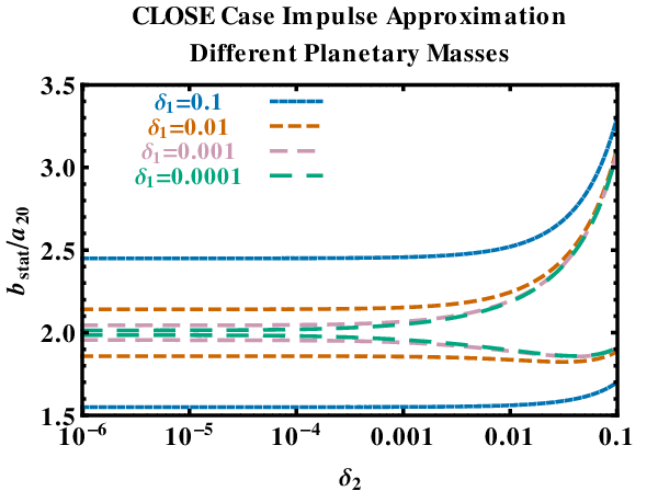
Here we briefly consider how orbital parameters might be perturbed when the planetary masses are unequal. The ratio of planetary masses should be most important when the planets are near each other during the close encounter of the two systems. Therefore, let us consider the close configuration, and specifically focus on the region around the planet-planet collision point (roughly bounded by $b_{{\rm stat},<}$ and $b_{{\rm stat},>}$ )

Denote $\delta_{1}\equiv M_{p1}/M_{s1}$ and $\delta_{2}\equiv M_{p2}/M_{s2}$ . For simplicity, choose $M_{s1}=M_{s2}$ and $a_{10}=a_{20}$ , as in Section 3. If we carry out the same analytic procedure in that section and the Appendix, then we find that the eccentricity change of Planet #2 is similarly described by Eq. (17), except now:

	$\displaystyle Z_{4}$	$\displaystyle=$	$\displaystyle 2GM_{s1}V_{\infty}^{2}\left(6a_{20}-b\left(3-2\delta_{2}\right)\right)$		(48)
	$\displaystyle Z_{5}$	$\displaystyle=$	$\displaystyle V_{\infty}^{4}\left(4a_{20}^{2}+b^{2}\left(1-2\delta_{2}\right)-ba_{20}\left(4+\delta_{1}-3\delta_{2}\right)\right)$		(49)

The result is the critical points around the planet-planet collision region become:

	$\displaystyle b_{{\rm stat,<}}^{(c)}$	$\displaystyle\approx$	$\displaystyle a_{20}\left[\frac{4-\sqrt{\delta_{1}^{2}+\delta_{1}\left(8-6\delta_{2}\right)+\delta_{2}\left(8+9\delta_{2}\right)}}{2-4\delta_{2}}\right]$		(50)
	$\displaystyle b_{{\rm stat,>}}^{(c)}$	$\displaystyle\approx$	$\displaystyle a_{20}\left[\frac{4+\sqrt{\delta_{1}^{2}+\delta_{1}\left(8-6\delta_{2}\right)+\delta_{2}\left(8+9\delta_{2}\right)}}{2-4\delta_{2}}\right]$		(51)

which is equivalent to Eqs. (66)-(67) when $\delta_{1}=\delta_{2}$ .

We plot these critical points as functions of the mass ratios in Fig. 20. The plot demonstrates that given a Jupiter-mass Planet #1, the region of planet-planet gravitational influence changes by $\approx 0.1a_{20}$ if Planet #2’s mass is an Earth-mass versus a Jupiter-mass. In the latter case, the region of influence is greater. Note also how the asymmetry of the two critical $b_{\rm stat}$ points is enhanced when the planetary masses approach the stellar masses.

6.2 Other System Configurations

Scattering simulations for different hierarchical configurations of 4 bodies, or for more than 4 bodies, would provide a more complete picture of planetary orbital excitation from passing stars during the host star’s middle age. However, the phase space to be explored is prohibitive. Nevertheless, because the few-body problem admits few analytical solutions, studies often must rely on numerical integrations.

Alternatively, in the Galactic Disc, the impulse formalism may be generalized to any number of bodies in any orientations. Although the resulting analytical formulas are unlikely to be as compact as those presented here, they – subject to the assumption in Eq. (7) – would be able to sample the entire phase space. Such a formalism could be useful, for example, in modeling how secular or resonant evolution of multi-planet systems might change naturally over time. Zakamska & Tremaine (2004) consider secular eccentricity propagation. For resonant systems, this same propagation might kick planets into a deeper or shallower mean motion resonance, if not out of the resonance entirely. Results from the Kepler mission illustrate that there is an abundance of near-resonant planets (Lissauer et al., 2011; Fabrycky et al., 2012).

In cases other than the close and far cases, impulses would cause both a perpendicular and parallel kick. The net effect could be modelled as a single impulse. If a planet is on an eccentric orbit before the kick, then the true anomaly of the planet must be taken into account. In principle, one could remove the error bars associated with Poisson counting statistics in Figs. 7-11 by generating those figures analytically, and then generalizing the figures with a given distribution of eccentricities. In this way, one can also quantify the preference of a planet’s eccentricity to increase versus decrease given an initial nonzero value.

This formalism should also work for hierarchical systems: those with stars, planets and moons. The Solar System demonstrates that moons typically orbit planets within half of a Hill radius. Further, a planet’s Hill radius is proportional to its semimajor axis. Therefore, wide orbit planets with moons⁵⁵ 5 Wide-orbit planets scattered out to their current locations could have retained moons, whether the moons were formed in the circumplanetary disc or were captured satellites. could feature a widely spaced moon orbit, one which extends to several percent of the planet’s semimajor axis. At a distance of 1000 AU, such an orbit would be comparable to the Neptune-Sun separation, and hence could be disrupted by passing stars.

Also, given the possible vast population of free-floating giant planets (Sumi et al., 2011), passing giant planets might be more common than passing stars. Then, the resulting binary-single interactions with a passing free-floater and a planetary system could become important (Varvoglis et al., 2012). If a giant free-floating planet of mass $M_{p}$ were to pass by a system with a planet of mass $M_{p}$ orbiting a star of mass $M_{s}$ , then the critical velocity of this configuration is $\sqrt{(2\delta+1)/(2+\delta)}\approx 71\%$ of the critical velocity of the traditional stellar flyby binary-single scattering configuration. This reduction in $V_{\rm crit}$ is not enough to claim that the system will be completely ionized; hence, this situation may be treated in a similar impulse situation as this work. In the perhaps more exotic situation of two pairs of free-floating planet binaries suffering a close encounter, $V_{\rm crit}$ would be reduced from the traditional four-star encounter by a factor of $1/\sqrt{\delta}\approx 32$ . This reduction is significant enough that ionization would be much more likely in that case for typical Galactic field velocities.

7 Conclusion

We have modeled the close encounter of two single-planet exosystems in the Galactic Disc, which mimicks a common occurence during middle-aged planetary evolution. We obtained analytical formulae and numerical cross sections which may be useful for future population studies of exoplanets in specific regions of the Milky Way. The resulting change in orbital parameters for wide-orbit ( $a\approx 100-1000$ AU) planets is significant (with a typical $\Delta e$ of several hundredths to over a tenth) and potentially measurable, suggesting that these planets are highly unlikely to retain a static orbit during main sequence evolution. Although tight-orbit planets (with $a\lesssim 10$ AU) are more resistant to orbital changes, millions in the Milky Way will be affected, and lose their primordial orbital signatures. The most dynamically excited Milky Way exoplanets are likely to reside in the densest Galactic regions.

Acknowledgments

We thank the referee for a careful read of the manuscript and astute and helpful suggestions.

References

Abt (2001) Abt, H. A. 2001, AJ, 122, 2008
Antoja et al. (2011) Antoja, T., Figueras, F., Romero-Gómez, M., et al. 2011, MNRAS, 418, 1423
Bacon et al. (1996) Bacon, D., Sigurdsson, S., & Davies, M. B. 1996, MNRAS, 281, 830
Bennett et al. (2012) Bennett, D. P., Sumi, T., Bond, I. A., et al. 2012, arXiv:1203.4560
Binney et al. (2000) Binney, J., Dehnen, W., & Bertelli, G. 2000, MNRAS, 318, 658
Binney & Tremaine (1987) Binney, J., & Tremaine, S. 1987, Princeton, NJ, Princeton University Press, 1987, 747 p.,
Bekki & Freeman (2003) Bekki, K., & Freeman, K. C. 2003, MNRAS, 346, L11
Binney & Tremaine (2008) Binney, J., & Tremaine, S. 2008, Galactic Dynamics: Second Edition, by James Binney and Scott Tremaine. ISBN 978-0-691-13026-2 (HB). Published by Princeton University Press, Princeton, NJ USA, 2008.
Boley et al. (2012) Boley, A. C., Payne, M. J., & Ford, E. B. 2012, arXiv:1204.5187
Carollo et al. (2007) Carollo, D., Beers, T. C., Lee, Y. S., et al. 2007, Nature, 450, 1020
Cassan et al. (2012) Cassan, A., Kubas, D., Beaulieu, J.-P., et al. 2012, Nature, 481, 167
Davies & Sigurdsson (2001) Davies, M. B., & Sigurdsson, S. 2001, MNRAS, 324, 612
De Simone et al. (2004) De Simone, R., Wu, X., & Tremaine, S. 2004, MNRAS, 350, 627
Duncan et al. (1987) Duncan, M., Quinn, T., & Tremaine, S. 1987, AJ, 94, 1330
Fabrycky et al. (2012) Fabrycky, D. C., Lissauer, J. J., Ragozzine, D., et al. 2012, arXiv:1202.6328
Fregeau et al. (2004) Fregeau, J. M., Cheung, P., Portegies Zwart, S. F., & Rasio, F. A. 2004, MNRAS, 352, 1
Fregeau et al. (2006) Fregeau, J. M., Chatterjee, S., & Rasio, F. A. 2006, ApJ, 640, 1086
Giersz & Spurzem (2003) Giersz, M., & Spurzem, R. 2003, MNRAS, 343, 781
Goldman et al. (2010) Goldman, B., Marsat, S., Henning, T., Clemens, C., & Greiner, J. 2010, MNRAS, 405, 1140
Gómez et al. (2010) Gómez, F. A., Helmi, A., Brown, A. G. A., & Li, Y.-S. 2010, MNRAS, 408, 935
Heggie & Rasio (1996) Heggie, D. C., & Rasio, F. A. 1996, MNRAS, 282, 1064
Heggie (2000) Heggie, D. C. 2000, MNRAS, 318, L61
Helmi et al. (1999) Helmi, A., White, S. D. M., de Zeeuw, P. T., & Zhao, H. 1999, Nature, 402, 53
Howe & Clarke (2009) Howe, K. S., & Clarke, C. J. 2009, MNRAS, 392, 448
Huang & Wade (1966) Huang, S.-S., & Wade, C., Jr. 1966, ApJ, 143, 146
Hurley et al. (2000) Hurley, J. R., Pols, O. R., & Tout, C. A. 2000, MNRAS, 315, 543
Hut (1993) Hut, P. 1993, ApJ, 403, 256
Hut & Bahcall (1983) Hut, P., & Bahcall, J. N. 1983, ApJ, 268, 319
Jackson & Wyatt (2012) Jackson, A. P., & Wyatt, M. C. 2012, arXiv:1206.4190
Kokubo et al. (1998) Kokubo, E., Yoshinaga, K., & Makino, J. 1998, MNRAS, 297, 1067
Kuzuhara et al. (2011) Kuzuhara, M., Tamura, M., Ishii, M., Kudo, T., Nishiyama, S., & Kandori, R. 2011, AJ, 141, 119
Lépine et al. (2011) Lépine, J. R. D., Roman-Lopes, A., Abraham, Z., Junqueira, T. C., & Mishurov, Y. N. 2011, MNRAS, 414, 1607
Lissauer et al. (2011) Lissauer, J. J., Ragozzine, D., Fabrycky, D. C., et al. 2011, ApJS, 197, 8
Luhman et al. (2011) Luhman, K. L., Burgasser, A. J., & Bochanski, J. J. 2011, ApJL, 730, L9
Malmberg et al. (2011) Malmberg, D., Davies, M. B., & Heggie, D. C. 2011, MNRAS, 411, 859
Mikkola (1984) Mikkola, S. 1984, MNRAS, 207, 115
Moeckel & Veras (2012) Moeckel, N., & Veras, D. 2012, MNRAS, 2631
Nakajima et al. (2010) Nakajima, T., Morino, J.-I., & Fukagawa, M. 2010, AJ, 140, 713
Nakajima & Morino (2012) Nakajima, T., & Morino, J.-I. 2012, AJ, 143, 2
Parravano et al. (2011) Parravano, A., McKee, C. F., & Hollenbach, D. J. 2011, ApJ, 726, 27
Perets & Kouwenhoven (2012) Perets, H. B., & Kouwenhoven, M. B. N. 2012, arXiv:1202.2362
Pfahl & Muterspaugh (2006) Pfahl, E., & Muterspaugh, M. 2006, ApJ, 652, 1694
Quillen et al. (2011) Quillen, A. C., Dougherty, J., Bagley, M. B., Minchev, I., & Comparetta, J. 2011, MNRAS, 417, 762
Roy (2005) Roy, A. E. 2005, Orbital motion / A. E. Roy. Bristol (UK): Institute of Physics Publishing, 4th edition. ISBN 0-7503-1015-6, 2005, XVIII + 526 pp.,
Schoenrich (2011) Schoenrich, R. 2011, arXiv:1111.3651
Setiawan et al. (2010) Setiawan, J., Klement, R. J., Henning, T., et al. 2010, Science, 330, 1642
Spiegel et al. (2011) Spiegel, D. S., Burrows, A., & Milsom, J. A. 2011, ApJ, 727, 57
Spurzem et al. (2009) Spurzem, R., Giersz, M., Heggie, D. C., & Lin, D. N. C. 2009, ApJ, 697, 458
Sumi et al. (2011) Sumi, T., Kamiya, K., Bennett, D. P., et al. 2011, Nature, 473, 349
Sweatman (2007) Sweatman, W. L. 2007, MNRAS, 377, 459
Taff (1985) Taff, L. G. 1985, New York, Wiley-Interscience, 1985, 540 p.,
Varvoglis et al. (2012) Varvoglis, H., Sgardeli, V., & Tsiganis, K. 2012, arXiv:1201.1385
Veras et al. (2009) Veras, D., Crepp, J. R., & Ford, E. B. 2009, ApJ, 696, 1600
Veras et al. (2011) Veras, D., Wyatt, M. C., Mustill, A. J., Bonsor, A., & Eldridge, J. J. 2011, MNRAS, 417, 2104
Veras & Raymond (2012) Veras, D., & Raymond, S. N. 2012, MNRAS, 421, L117
Veras & Tout (2012) Veras, D., & Tout, C. A. 2012, MNRAS, 2678
Welsh et al. (2012) Welsh, W. F., Orosz, J. A., Carter, J. A., et al. 2012, Nature, 481, 475
Wolszczan (1994) Wolszczan, A. 1994, Science, 264, 538
Yuan & Kuo (1997) Yuan, C., & Kuo, C.-L. 1997, ApJ, 486, 750
Zakamska & Tremaine (2004) Zakamska, N. L., & Tremaine, S. 2004, AJ, 128, 869

Appendix A Additional Analytics

This Appendix expounds upon the analytical results in Section 3. The resulting formulae may be applied generally to a particular exosystem of study, and contribute to our analytic understanding of the general four-body problem.

We can relate the effective impact parameters to the closest approach distances of all of the planet-star combinations through geometry. We obtain:

$\displaystyle b_{s1p2}$	$\displaystyle=$	$\displaystyle\left(q\pm a_{10}\right)\frac{bV_{\infty}^{2}}{\mu}\left[1+\left(\frac{bV_{\infty}^{2}}{\mu}\right)^{2}\right]^{-\frac{1}{2}}$	(52)
$\displaystyle b_{p1s2}$	$\displaystyle=$	$\displaystyle\left(q\pm a_{20}\right)\frac{bV_{\infty}^{2}}{\mu}\left[1+\left(\frac{bV_{\infty}^{2}}{\mu}\right)^{2}\right]^{-\frac{1}{2}}$	(53)
$\displaystyle b_{p1p2}$	$\displaystyle=$	$\displaystyle\left(q\pm a_{10}\pm a_{20}\right)\frac{bV_{\infty}^{2}}{\mu}\left[1+\left(\frac{bV_{\infty}^{2}}{\mu}\right)^{2}\right]^{-\frac{1}{2}}$	(54)

where the upper and lower signs correspond to the far and close cases, respectively. In the close case, $b_{\rm min}$ is the value of $b$ which gives $b_{p1p2}=0$ . Eq. (3) yields:

b_{\rm min}=\sqrt{\left(a_{10}+a_{20}\right)\left(a_{10}+a_{20}+\frac{2G\mu}{V_{\infty}^{2}}\right)}

(55)

When $b<b_{\rm min}$ , then $b_{p1p2}<0$ and the systems cross orbits. For a low enough $b$ (when $b_{s1p2}<0$ or $b_{p1s2}<0$ ), the stars directly pass through the region in-between the other system’s planetary orbit.

Now we impose the analytic simplification described in Section 3.2.1 and apply the fiducial values from Section 3.2.2 to accompany the analytics.

To gain physical insight into the following situations, consider how the perpendicular impulses from Eqs. (8) - (11) tend toward zero for both $b\rightarrow 0$ and $b\rightarrow\infty$ . Therefore, each impulse is maximized for a particular finite value of $b$ . These values are given by:

$\displaystyle b_{{\rm crit},s1s2}$	$\displaystyle=$	$\displaystyle\frac{G\mu}{V_{\infty}^{2}}$
$\displaystyle b_{{\rm crit},s1p2}$	$\displaystyle=$	$\displaystyle b_{{\rm crit},p1s2}$
	$\displaystyle=$	$\displaystyle\sqrt{\left(\frac{\left(1+\delta\right)GM_{S1}}{V_{\infty}^{2}}\pm a_{20}\right)\left(\frac{\left(5+\delta\right)GM_{S1}}{V_{\infty}^{2}}\pm a_{20}\right)}$
$\displaystyle b_{{\rm crit},p1p2}$	$\displaystyle=$	$\displaystyle 2\sqrt{\left(\frac{\delta GM_{S1}}{V_{\infty}^{2}}\pm a_{20}\right)\left(\frac{\left(2+\delta\right)GM_{S1}}{V_{\infty}^{2}}\pm a_{20}\right)}$

where the upper and lower signs denote the far and close cases, respectively. For planetary systems, $\delta$ is small and hence the expressions for $b_{{\rm crit},s1p2}$ and $b_{{\rm crit},p1p2}$ may be shortened. For the fiducial values we adopted above, $b_{{\rm crit},s1s2}\approx 1.97$ AU, very close to the collision point of the stars. Further, in the far case, $b_{{\rm crit},s1p2}^{(f)}\approx 997.04$ AU and $b_{{\rm crit},p1p2}^{(f)}\approx 1998.03$ AU, which are both a few AU away from $a_{10}=a_{20}$ . In the close case, $b_{{\rm crit},s1p2}^{(c)}\approx 1002.96$ AU and $b_{{\rm crit},p1p2}^{(c)}\approx 2001.97$ AU. In this case, note further that when $\delta=0$ , then $b_{{\rm crit},p1p2}^{(c)}=b_{\rm min}$ ; otherwise, $b_{{\rm crit},p1p2}^{(c)}$ is slightly higher:

	$\displaystyle\frac{b_{{\rm crit},p1p2}^{(c)}}{b_{\rm min}}$	$\displaystyle\approx$	$\displaystyle 1+2\delta\left(\frac{a_{20}}{b_{\rm min}}\right)^{2}\left(\frac{V_{{\rm circ},0}}{V_{\infty}}\right)^{2}$		(56)
		$\displaystyle\times$	$\displaystyle\left[2+\left(2+\delta\right)\left(\frac{V_{{\rm circ},0}}{V_{\infty}}\right)^{2}\right]$		(56)

For our fiducial case, $b_{{\rm crit},p1p2}^{(c)}-b_{\rm min}\approx 0.0019$ AU $=2.8\times 10^{5}$ km, which is smaller than the radius of the Sun but not of any of the Solar System planets.

These critical values interact with one another to produce the interesting dynamics below. We first consider the far case.

In the limit of $b=0$ , the stars will collide and impart a large perpendicular kick to the planets. The kick will be greatest at $b=b_{{\rm crit},s1s2}$ , which is about only $0.2\%$ of $a_{20}$ for our fiducial case. Nevertheless, reductions of Eqs. (13) and (14) show that the planet will be ejected ( $a_{2f}\rightarrow\infty$ , $e_{2f}\geq 1$ ) for all $b$ from 0 to $b_{{\rm eje}}^{(f)}$ , where

b_{{\rm eje}}^{(f)}\approx\frac{a_{20}}{2V_{\infty}}\left[2V_{{\rm circ},0}-V_{\infty}+\sqrt{V_{\infty}\left(V_{\infty}+12V_{{\rm circ},0}\right)}\right]

(57)

or, at about $118$ AU for our fiducial case. This result shows how a passing star at $\sim 100$ AU can rip a bound planet off of another star, even if the passing star is at opposition with the other star’s planet.

The eccentricity and semimajor axis perturbations approximated by Eqs. (15)-(16) are independent of planetary mass because, in this case the planets are always “far” ( $\geq 2a_{20}=2000$ AU $\gtrsim b_{{\rm crit},p1p2}^{(f)}$ ) from each other.⁶⁶ 6 Equation (15) does not reduce to Eqs. (9) or (11) of Heggie & Rasio (1996) because the assumptions used to derive those latter two formulas are different: encounters are assumed to be slow, the encounter trajectory is assumed to be parabolic, and the impact parameter is assumed to be large relative to the planet-star semimajor axes. Further, the power-law dependence is reported in terms of pericenter distance. Similarly, because $b_{{\rm eje}}^{(f)}+a_{20}>b_{{\rm crit},p1p2}^{(f)}$ , we should expect the eccentricity and semimajor axis distributions to be smooth functions of $b>b_{{\rm eje}}^{(f)}$ .

This formalism allows us to estimate the contribution to Planet #2’s eccentricity variation from the potential of Planet #1 alone:

	$\displaystyle e_{\chi}^{(f)}$	$\displaystyle\equiv$	$\displaystyle\left\|\frac{\|\Delta\vec{V}_{\bot}\|_{p1s2}-\|\Delta\vec{V}_{\bot}\|_{p1p2}}{\|\Delta\vec{V}_{\bot}\|_{p2}}\right\|$		(58)
		$\displaystyle\approx$	$\displaystyle\left\|\frac{\delta b^{2}}{2b\delta\left(b+a_{20}\right)-\left(b+2a_{20}\right)^{2}}\right\|$		(59)

Equation (59) shows that the relative contribution from the planet is an increasing function of $b$ . The maximum contribution is

e_{\chi_{\rm max}}^{(f)}=e_{\chi}^{(f)}(b\rightarrow\infty)=\frac{\delta}{1-2\delta}

(60)

showing that Planet #1 completely dominates the evolution when $\delta=1/3$ . Similarly, we can quantify the change in Planet #2’s semimajor axis from Planet #1 alone:

	$\displaystyle a_{\chi}^{(f)}$	$\displaystyle\equiv$	$\displaystyle\frac{\left(a_{2f}-a_{20}\right)_{\rm Planet\ \#1\ Only}}{\left(a_{2f}-a_{20}\right)_{\rm Total}}=\frac{e_{\chi}^{{(f)}^{2}}\left(1-e_{2f}^{{(f)}^{2}}\right)}{1-e_{2f}^{{(f)}^{2}}e_{\chi}^{{(f)}^{2}}}$		(61)
		$\displaystyle=$	$\displaystyle\delta^{2}b^{2}\left[\frac{\left(bZ_{1}\right)^{2}-\left(Z_{2}\right)^{2}}{\left(Z_{1}Z_{3}\right)^{2}-\left(\delta bZ_{2}\right)^{2}}\right]$		(61)

where

$\displaystyle Z_{1}$	$\displaystyle=$	$\displaystyle\frac{b+a_{20}}{a_{20}}$	(62)
$\displaystyle Z_{2}$	$\displaystyle=$	$\displaystyle 2\left(b+2a_{20}\right)\frac{V_{{\rm circ},0}}{V_{\infty}}$	(63)
$\displaystyle Z_{3}$	$\displaystyle=$	$\displaystyle\left(b+2a_{20}\right)^{2}-2\delta b\left(b+a_{20}\right).$	(64)

Because it is expressed as differences of squares, Eq. (61) readily reveals the conditions that will zero out the planetary contribution.

Similar to the eccentricity, the relative contribution to $a_{2f}$ from the planet is an increasing function of $b$ . In the limit $b\rightarrow\infty$ ,

a_{\chi_{\rm max}}^{(f)}=\left(\frac{\delta}{1-2\delta}\right)^{2}

(65)

again showing that Planet #1 completely dominates the evolution when $\delta=1/3$ . Comparing $a_{\chi_{\rm max}}^{(f)}$ and $e_{\chi_{\rm max}}^{(f)}$ suggests that intruding planets have a greater capacity to alter other planets’ eccentricities than their semimajor axes.

Figure 21 graphically illustrates Planet #1’s contribution to the evolution of Planet #2 in the far case. The plots demonstrate the contrastingly weak and strong dependencies of $e_{\chi}^{(f)}$ and $a_{\chi}^{(f)}$ on $V_{\infty}$ and $\delta$ , respectively. Also, $e_{\chi}^{(f)}>a_{\chi}^{(f)}$ always. For the most massive-possible exoplanets ( $\approx 11M_{J}-16M_{J}$ ; Spiegel et al. 2011) and impact parameters of a few thousand AU, the planetary contribution may reach $10\%$ of the overall contribution.

Now we perform a similar analysis for the close case. Here, where the position vectors from each star to their orbiting planet point towards each other, the resulting orbital parameter evolution is a more complicated function of $b$ . Figures 6 and 22 may be helpful guides for the following discussion.

In the limiting case of $b=b_{\rm min}$ , the planets collide with each other, and the kicks on each other have no perpendicular component (as can be seen in Eq. 11). Further, the perpendicular kicks from both stars would cancel out. Therefore, in this limit – if the collision could be neglected – the planets’ orbital parameters would remain nearly unchanged. However, even a slight nonzero distance between the planets would produce strong perpendicular kicks, much stronger than the kicks from the stars, and cause the planets to escape. This kick is highest at $b_{{\rm crit},p1p2}^{(c)}$ , which differs from $b_{\rm min}$ on the order of a giant planet radius (Eq. 56). Therefore, around the vicinity of $b_{\rm min}$ , the planets either collide with each other or escape.

As $b$ deviates from $b_{\rm min}$ , eventually the kick contributions from both Star #1 and Planet #1 will cancel out the back reaction from Star #1 on Star #2. The result is that planet’s orbital elements would remain unchanged. This situation occurs at:

	$\displaystyle b_{{\rm stat,<}}^{(c)}$	$\displaystyle\approx$	$\displaystyle a_{20}\left[\frac{2-\sqrt{\delta\left(4+\delta\right)}}{1-2\delta}\right]$		(66)
	$\displaystyle b_{{\rm stat,>}}^{(c)}$	$\displaystyle\approx$	$\displaystyle a_{20}\left[\frac{2+\sqrt{\delta\left(4+\delta\right)}}{1-2\delta}\right]$		(67)

where the subscripts $<$ and $>$ indicate that $b_{{\rm stat}}$ is less than or greater than $b_{\rm min}$ . For our fiducial case, $b_{{\rm stat,<}}^{(c)}\approx 1942$ AU and $b_{{\rm stat,>}}^{(c)}\approx 2066$ AU.

For $b<b_{{\rm stat,<}}$ , the perturbation on Planet #2 becomes high as Star #1 approaches. In the vicinity of $b\approx a_{20}$ , where Planet #2 collides with Star #1, the planet is either ejected or destroyed for $b_{{\rm eje,2}}\leq b\leq b_{{\rm eje,1}}$ , where

b_{{\rm eje,2}}^{(c)}\approx\frac{a_{20}}{2V_{\infty}}\left[2V_{{\rm circ},0}+V_{\infty}+\sqrt{V_{\infty}\left(V_{\infty}-12V_{{\rm circ},0}\right)}\right],

(68)

b_{{\rm eje,1}}^{(c)}\sim 2a_{20}-b_{{\rm eje,2}}^{(c)}.

(69)

For our fiducial case, $b_{{\rm eje,1}}^{(c)}\sim 1074$ AU and $b_{{\rm eje,2}}^{(c)}\approx 926$ AU. For $b<b_{{\rm eje,2}}^{(c)}$ , the perturbations on Planet #2 stay high as the two stars approach each other (bottom panel of Fig. 4). The planet will escape for $b<b_{{\rm eje,3}}^{(c)}$ , where

b_{{\rm eje,3}}^{(c)}\approx\frac{a_{20}}{2V_{\infty}}\left[2V_{{\rm circ},0}+V_{\infty}-\sqrt{V_{\infty}\left(V_{\infty}-12V_{{\rm circ},0}\right)}\right]

(70)

In our fiducial case, $b_{{\rm eje,3}}^{(c)}\approx 137$ AU. In between $b_{{\rm eje,2}}^{(c)}$ and $b_{{\rm eje,3}}^{(c)}$ , the eccentricity and semimajor axis variations are minimized at

b_{{\rm ext,min}}^{(c)}\approx\left(2-\sqrt{2}\right)a_{20}\left[1+2\left(\frac{V_{{\rm circ},0}}{V_{\infty}}\right)^{2}\right]

(71)

or, a value of $\approx 587$ AU for our fiducial case. The resulting minimum eccentricity and semimajor axes values are

	$\displaystyle e_{\rm ext,min}^{(c)}$	$\displaystyle\approx$	$\displaystyle\left(6+4\sqrt{2}\right)\left(\frac{V_{{\rm circ},0}}{V_{\infty}}\right),$		(72)
	$\displaystyle a_{\rm ext,min}^{(c)}$	$\displaystyle\approx$	$\displaystyle a_{20}\left[1-\left(6+4\sqrt{2}\right)^{2}\left(\frac{V_{{\rm circ},0}}{V_{\infty}}\right)^{2}\right]^{-1}$		(73)

or $e_{\rm ext,min}^{(c)}=0.366$ and $a_{\rm ext,min}^{(c)}=1.155a_{20}$ . Eqs. (72) and (73) imply that Planet #2 cannot remain bound at any $b<b_{{\rm eje,1}}^{(c)}$ if $V_{\infty}\leq 11.7V_{{\rm circ},0}\approx 10.8{\rm km/s}$ . Therefore, Fig. 6 does not feature a black solid curve (which represents $V_{\infty}=10\ {\rm km/s}$ ) for $b\lesssim 1074$ AU in either panel. However, when using this critical relation, one should remember that the impulse approximation starts to break down as $V_{\infty}$ decreases according to Eq. (7).

Now let us consider $b>b_{{\rm stat,>}}^{(c)}$ . In this regime, the planet-planet interaction becomes negligible, and Planet #2’s evolution is dominated by $|\Delta\vec{V}_{\bot}|_{s1s2}$ and $|\Delta\vec{V}_{\bot}|_{s1p2}$ . These impulses partially, but not completely, cancel each other out, and admit the greatest net perturbation on Planet #2 at

b_{{\rm ext,max}}^{(c)}\approx\left(2+\sqrt{2}\right)a_{20}\left[1+2\left(\frac{V_{{\rm circ},0}}{V_{\infty}}\right)^{2}\right]

(74)

or $\approx 3421$ AU, which correspondingly results in maximum eccentricity and semimajor axes values of

	$\displaystyle e_{\rm ext,max}^{(c)}$	$\displaystyle\approx$	$\displaystyle\left(6-4\sqrt{2}\right)\left(\frac{V_{{\rm circ},0}}{V_{\infty}}\right),$		(75)
	$\displaystyle a_{\rm ext,max}^{(c)}$	$\displaystyle\approx$	$\displaystyle a_{20}\left[1-\left(6-4\sqrt{2}\right)^{2}\left(\frac{V_{{\rm circ},0}}{V_{\infty}}\right)^{2}\right]^{-1}$		(76)

or $e_{\rm ext,max}^{(c)}\approx 0.011$ and $a_{\rm ext,max}^{(c)}=1.00012a_{20}$ . Equations (75) and (76) importantly let us explore if Planet #2 could ever be ejected when $b>a_{10}+a_{20}$ . Ejection is possible only if $V_{\infty}\leq 0.34V_{{\rm circ},0}\approx 0.32{\rm km/s}$ .

Finally, to complete our exploration of the impact parameter phase space, as $b\rightarrow\infty$ , the orbital changes asymptotically approach zero.

Planet #1 plays a much larger role in altering the orbit of Planet #2 in the close case instead of the far case. This can be seen by the dependence of $e_{2f}$ on $\delta$ , even though in route to the derivation of $e_{2f}$ , we neglected a higher order term due to $\delta$ . The fully general case (Eq. 14) makes no assumptions whatsoever about $\delta$ , meaning that the formula is just as applicable to four stars as it is to two stars and two planets. Hence, we use Eq. (14) in order to plot Fig. 22, which illustrates the dependence on $\delta$ .

The plot provides an effective region of planet-planet influence, perhaps interpreted as the region where planet-planet gravitational focusing is important. For $\delta=0.1$ , this region is nearly as large as $0<b<b_{{\rm stat,<}}^{(c)}$ . Note however, that the orbital parameter variations for $b<b_{{\rm stat,<}}^{(c)}$ are nearly completely independent of $\delta$ . For $b>b_{{\rm stat,<}}^{(c)}$ , greater values of $\delta$ have an overall weaker effect, because of the locations at which the forces partially cancel out one another.

Now we can estimate what fraction of Planet #2’s orbital changes are due to Planet #1 alone. We find that $e_{\chi}^{(c)}$ is equal to

\frac{\delta b^{2}V_{\infty}^{2}\left(b-a_{20}\right)}{\left[2GM_{s1}+V_{\infty}^{2}\left(b-a_{20}\right)\right]\left[4a_{20}^{2}+b^{2}\left(1-2\delta\right)-2a_{20}b\left(2-\delta\right)\right]}

(77)

which takes the same limit of $\delta/(1-2\delta)$ for $b\rightarrow\infty$ as $e_{\chi}^{(f)}$ (Eq. 60). Similarly, the limit of $a_{\chi}^{(c)}$ as $b\rightarrow\infty$ is $\delta^{2}/(1-2\delta)^{2}$ . We plot these contributions in Fig. 23. The left and right panels illustrate the dependencies on $V_{\infty}$ and $\delta$ respectively. Like in the far case, here $e_{\chi}^{(f)}$ and $a_{\chi}^{(f)}$ are greatly sensitive to $\delta$ . Unlike in the far case, there is a region of impact parameter phase space where Planet #1’s contribution dominates the evolution. For $\delta\gtrsim 10^{-2}$ , the width of this region can extend beyond $10^{3}$ AU. Even for $b>10^{4}$ AU, the contribution due to massive exoplanets may still be a few percent of the overall contribution.