Spin Hall Conductivity on the Anisotropic Triangular Lattice

Let us now proceed with the diagonalization of the anisotropic TBH. We define the hopping amplitude in the $x$ and $0-4$ direction as $t=(2/3)t_{0}$ and that in the $0-5$ direction as $\tilde{t}=(2/3)\tilde{t}_{0}$. From now on, the lattice constant $a$ will be set to one, $a\equiv 1$.
The spectrum of the TBH is given by

where $F_{1}({\bf k})$ is defined as

The corresponding eigenvectors are

Before proceeding with the calculation of the SHC, let us first discuss some features of the energy spectrum which, as will be seen, will appear to be important and helpful to understand the characteristics of this dynamical quantity. As it is well known, the SHC can be directly related to the $k$-space curvature,[29] this will be presented in detail in what follows, Sec. III. In this context, the singular values of the Berry connection at degeneracy points of the energy spectrum are of crucial importance. To prepare the insight into the topological nature of this problem, we first calculate the degeneracies by solving directly $F_{1}(k)=0$. The result is plotted in Fig. 2.

In the absence of SOC ($t^{R}$=0) and in the isotropic case (${t_{0}}=\tilde{t}_{0}$), the density of states (DOS) exhibits a Van Hove singularity at Fermi energy $E=4/3t_{0}$. It corresponds to a straight line which goes through $P_{3}$ and $P_{5}$. For finite values of SOC strength, in the isotropic case, this peak is now split as clearly seen in Fig. 4. In addition, one has two additional peaks at the boundary of the energy spectrum.[30] The energy dispersion is plotted as a function of momentum in Fig. 3(d). As seen, the degeneracy points correspond to the points $P_{i}$ ($i=1,2,\ldots,5$) and $\Gamma$. One finds $E(P_{1})=E(P_{3})=E(P_{5})$ and $E(P_{2})=E(P_{4})$. In Fig. 4 these particular energies are indicated by dashed lines. When we switch on the anisotropy the singularities in the DOS change significantly as expected. In Fig. 3 one now sees that one degeneracy is lifted $E(P_{1})=E(P_{3})\neq E(P_{5})$, and we still have $E(P_{2})=E(P_{4})$. Thus in the presence of anisotropy we have four relevant energies that we denote,

with the energy expressed in values of $t_{0}$. Note that, two different sets of labels ($d_{1}$,$d_{2}$) and ($S_{1}$, $S_{2}$) are introduced. The meaning of this separation will become clear in what follows.

Having analyzed the energy spectrum, we now proceed further with the calculation of dynamical properties, more precisely the spin Hall conductivity $\sigma_{\text{SH}}$. The SHC is calculated within linear response theory using Kubo formula,[31, 32, 33, 30]

where $V$ is the total number of lattice sites, $E_{i}$ the eigenenergies, $\left|\psi_{i}\right\rangle$ the corresponding eigenstates, $E_{F}$ the Fermi energy and $\eta$ a positive infinitesimal. The spin current operator is

and the velocity is defined with the usual expression ${\bf v}=\mathit{i}[{\bf H,r}]$. To calculate the SHC we first compute the matrix element density function $j(x,y)$ defined by

where the matrix element $M_{mn}$ is

Note that the function $j(x,y)$ is a particularly useful and convenient quantity for calculations carried out by Kernel Polynomial Method[34] in the presence of disorder.[12, 35]

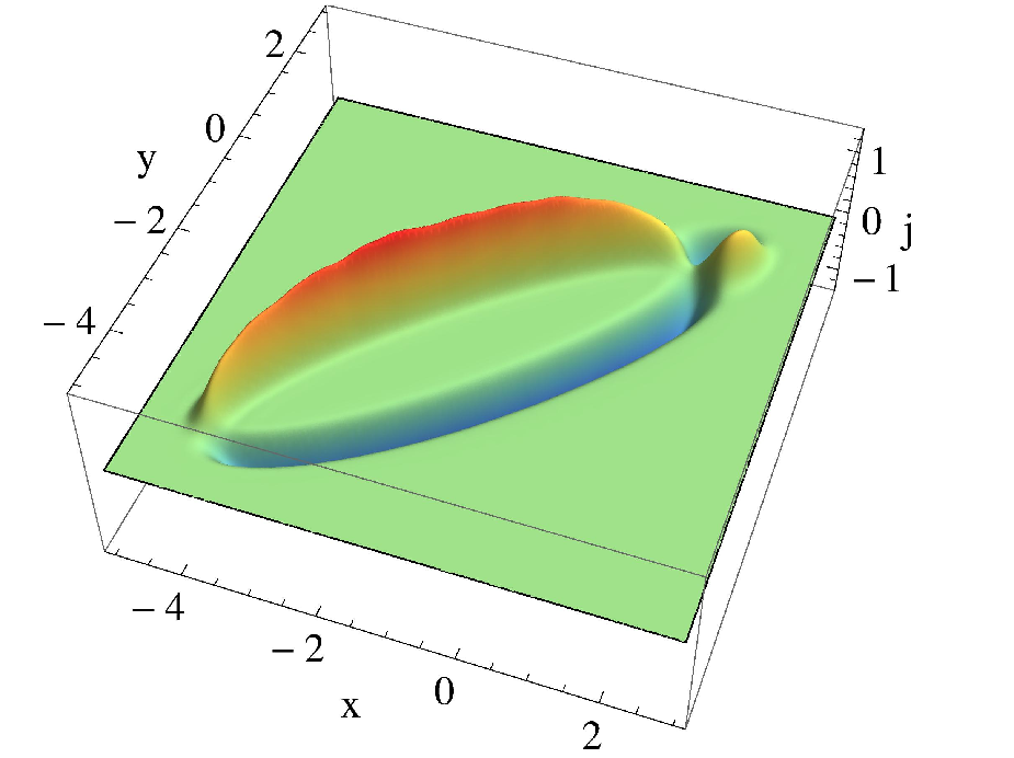
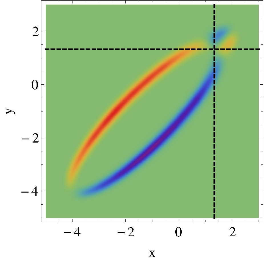
We can thus rewrite $\sigma_{\text{SH}}(E_{F})$ in terms of $j(x,y)$, leading to the following expression [12]:

where $f_{E_{F}}$ is the Fermi-Dirac distribution.

In the present case the only non-zero-matrix elements are

where

The function $j(x,y)$ is plotted in Fig. 5 for the isotropic case. Notice the symmetry due to Eq. 20. One can clearly see a sign change for $j$ values at $(x,y>x)$ resp. $(x,y<x)$. This gives a clear indication for a sign-change in $\sigma_{\text{SH}}$ at a particular Fermi level. In fact, this energy coincides with $E_{S1}$. The resulting SHC is plotted in Fig. 6. At low electron density we observe a sharp increase to $\sigma_{\text{SH}}=e/(8\pi)$ as expected since the lattice structure is irrelevant. As we increase the Fermi energy further, $\sigma_{\text{SH}}$ remains almost flat up to $E/t_{0}\approx 1$ (extended plateau). Then at $E=E_{S1}$ the sign of SHC changes in agreement with the discussion on $j(x,y)$. More remarkable is the change of amplitude of the SHC in the region of negative conductivity. Indeed, it increases by 60$\%$ with respect to the case of low electron density.

Interestingly, the calculations indicate that the finite size effects are almost negligible up to $E_{S1}$, but not in the hole doped regime. As mentioned before, one has to be careful in the derivation of TBH. We now compare the calculated SHC with that obtained using the TBH of Ref. 28. The result is plotted in Fig. 6 (b). As seen, the results are relatively comparable up to $E_{F}=-2t_{0}$ and drastically deviate in the vicinity of $E_{S1}$. The conductivity calculated within the TBH of Ref. 28 exhibits a clear maximum in the vicinity of $E_{S1}$, but no change of sign.

We now analyze the effect of anisotropy in the hopping amplitude on the SHC. The results are depicted in Fig. 7.

As we discussed it previously a change of sign occurs at $E_{S1}$. As we reduce $\tilde{t}_{0}$ we observe a shift of the crossing energy towards $E_{F}=0$. One also notices drastic changes in the shape of $\sigma_{\text{SH}}$ beyond $E_{S1}$. In particular, we observe two minima and a significant reduction of the amplitude of SHC. This is especially pronounced for the case $\tilde{t}_{0}=0.7t_{0}$. As the anisotropy is further decreased, the second minimum disappears and a second change of sign of the SHC is found. This occurs at the value of $\tilde{t}_{0}=(2/3)t_{0}$. Thus, below this value one has two changes of sign, one at $E_{S1}$ and the second at $E_{S2}$. One natural question which arises is why beyond this value SHC changes its sign a single time? This will be answered and understood when discussing the SHC in the framework of Berry phases. Remark that the second change of sign could not be anticipated from the DOS. Indeed, in contrast to the peak seen at $E_{S1}$ no peak, no singularity or pronounced feature is visible at $E_{S2}$, see for instance the case $\tilde{t}_{0}=(1/3)t_{0}$ in Fig. 4. The limiting case $\tilde{t}_{0}=0$ requires also some additional attention. In the absence of SOC, the system is topologically equivalent to the square lattice. As seen in Fig. 7 the results for $\sigma_{\text{SH}}$ are similar to that of the square lattice for $E_{F}<0$ (see e.g. Ref. 36, 37, 12). However, for $E_{F}>0$ (below $E_{F}/t_{0}<1$), the amplitude is reduced to half of that of the square lattice. The spin flip term in the $(2-5)$ direction at finite SOC is at the origin of these crucial differences in the hole doped regime. It is surprising that the drastic changes take place only for $E_{F}>0$, we will shed light on it in what follows.

In order to get a better understanding of the previously discussed features, we propose to analyze the results in the context of the Berry phase. As could be guessed from comparing the spectra shown in Fig. 3 and the SHC plotted in Fig. 7, the topology of the spectrum plays an important role in understanding the transport properties of electrons and their spins. We remind that the transport of a Bloch state $\left|\lambda(\bzeta)\right\rangle$ in the parameter space $\bzeta$ which has a non-vanishing curvature leads to picking up a geometrical phase. In the case of adiabatic transport, valid in the linear response regime, it is called Berry phase.[27] In momentum space this geometrical phase is at the origin of the quantum,[38, 39, 40] the anomalous[41] and spin[42, 43] Hall effects. The latter was also studied in the context of Fermi-surface topologies on honeycomb and kagome lattice by Liu et al. in Ref. 13, 14.
In our case the Berry phases are explicitly given by the integral

along a loop $C^{\pm}=\{k_{x},k_{y}\}$ in momentum space with the condition $E^{\pm}(k_{x},k_{y})=E_{F}$, the Berry connection ${\bf\mathcal{A}^{\pm}(k)}$ is

In our case we have found that ${\bf\mathcal{A}^{+}(k)}={\bf\mathcal{A}^{-}(k)}$. Indeed, the eigenvectors, Eq. 12, do not depend on the hopping anisotropy and therefore the Berry connection is independent of $\tilde{t}_{0}/t_{0}$. The Berry connection is shown as a stream plot in Fig. 8. Examining it in the vicinity of the degeneracy points of the energy spectrum, $\Gamma$ and $P_{i}$ $(i=1,\ldots,5)$, we find different winding directions for $\mathcal{A}$. It diverges exactly at these points. In order to relate our findings to the Berry connection we reformulate the SHC, Eq. (15), in terms of it,[44, 14]

where ${\bf v^{(0)}(k)}$ is the velocity in absence of SOC.
Let us show that the SHC sign is connected to that of $[{\bf\mathcal{A}}^{m}({\bf k})\times{\bf v^{(0)}(k)}]_{z}$. For that purpose we first consider the isotropic case.

Notice that below $E_{S1}$, as the term $(E_{+}({\bf k})-E_{-}({\bf k}))$ is always positive, the sign change of SHC is associated to that of $[{\bf\mathcal{A}}^{m}({\bf k})\times{\bf v^{(0)}(k)}]_{z}$. For $E_{F}<E_{S1}$ the winding direction is always clockwise for the Berry connection and the velocity is always pointing outside (see Fig. 9 (a)), resulting then in a positive SHC. Beyond $E_{S1}$ the Fermi surface topology is completely different, it consists now of closed loops around the $P_{2}$ and $P_{4}$ as illustrated in Fig. 9 (b). Furthermore, the direction of the velocity is now directed inside (towards $P_{2}$ and $P_{4}$). However, the winding directions (see Fig. 8) of the Berry connection is unchanged, clockwise as around the $\Gamma$ point. This results in a sign change of the spin Hall conductivity. We now proceed further and discuss the presence of anisotropy. Since as mentioned before, $\mathcal{A}$ is independent of $\tilde{t}_{0}$ thus the changes in SHC are associated with the Fermi surface topology only. Let us start with the extreme case of a fully anisotropic system, e.g. $\tilde{t}_{0}=0$. As seen before, the SHC exhibits two changes of sign, one at $E_{S1}$ and the other at $E_{S2}$. Thus, we focus our attention on these two Fermi energies. The situation at $E_{S1}$, Fig. 10 (a) and (b), is very similar to that of the isotropic case, except the fact that the Fermi surface at $E_{F}=E_{S1}+\epsilon$ is now also surrounding the point $P_{5}$ for which the winding direction of Berry connection is now negative (anti-clockwise).

As the velocity direction is still pointing inwards, the negative winding around $P_{5}$ can lead to a sign change in $[{\bf\mathcal{A}}^{m}({\bf k})\times{\bf v^{(0)}(k)}]_{z}$, thus, to the appearance of terms in Eq. 25 which reduce the absolute value of $\sigma_{\text{SH}}$. This explains why $\sigma_{\text{SH}}$ varies from $\sim-1.6e/(8\pi)$ in the isotropic case to $\sim-0.5e/(8\pi)$ for $\tilde{t}_{0}=0$ . Concerning the second sign change, we find at $E_{F}=E_{S2}\pm\epsilon$ the same velocity direction. However, the Fermi surface at $E_{F}=E_{S2}+\epsilon$ is, in contrast to Fig. 10 (b) and (c), surrounding only $P_{5}$ which as mentioned before has the opposite winding direction with respect to that of $P_{2}$ and $P_{4}$. This yields the topological explanation of the change of sign at $E_{S2}$.

References

- [1] S. Datta and B. Das, Appl. Phys. Lett. 56, 665 (1990).
- [2] Y. Bychkov and E. Rashba, JETP Lett. 39, 78 (1984).
- [3] E. Rashba, Sov. Phys.-Solid State 2, 1109 (1960).
- [4] G. Dresselhaus, Phys. Rev. 100, 580 (1955).
- [5] M. I. D’yakonov and V. I. Perel’, JETP Lett. 13, 467 (1971).
- [6] J. Schliemann, IJMPB 20 (2006).
- [7] J. Wunderlich, B. Kaestner, J. Sinova, and T. Jungwirth, Phys. Rev. Lett. 94, 047204 (2005).
- [8] Y. K. Kato, R. C. Myers, A. C. Gossard, and D. D. Awschalom, Science (New York, N.Y.) 306, 1910 (2004).
- [9] H.-A. Engel, E. I. Rashba, and B. I. Halperin, MaterialsTheory of Spin Hall Effects in Semiconductors (John Wiley & Sons, Ltd, Cambridge, MA, USA, 2007), ISBN 0470022175.
- [10] C. Brüne, A. Roth, E. G. Novik, M. König, H. Buhmann, E. M. Hankiewicz, W. Hanke, J. Sinova, and L. W. Molenkamp, Nature Physics 6, 448 (2010).
- [11] J. Sinova, D. Culcer, Q. Niu, N. A. Sinitsyn, T. Jungwirth, and A. H. MacDonald, Phys. Rev. Lett. 92 (2004).
- [12] P. Wenk, Ph.D. thesis, Jacob University Bremen (2011).
- [13] G. Liu, Z. Wang, and S.-S. Li, Physics Letters A 373, 2091 (2009a).
- [14] G. Liu, P. Zhang, Z. Wang, and S.-S. Li, Phys. Rev. B 79, 035323 (2009b).
- [15] K. Penc, H. Shiba, F. Mila, and T. Tsukagoshi, Phys. Rev. B 54, 4056 (1996).
- [16] Y. Watanabe and S. Miyashita, J. Phys. Soc. Jpn. 66, 2123 (1997).
- [17] O. Derzhko, J. Richter, A. Honecker, M. Maksymenko, and R. Moessner, Phys. Rev. B 81, 014421 (2010).
- [18] A. Mielke, J. Phys. A: Math. Gen. 24, 3311 (1991).
- [19] A. Mielke, J. Phys. A: Math. Gen. 25, 4335 (1992).
- [20] H. Tasaki, Phys. Rev. Lett. 69, 1608 (1992).
- [21] A. Mielke and H. Tasaki, Commun. Math. Phys. 158, 341 (1993).
- [22] C. Becker, P. Soltan-Panahi, J. Kronjäger, S. Dörscher, K. Bongs, and K. Sengstock, New Journal of Physics 12, 065025 (2010).
- [23] R. G. Melko, A. Paramekanti, A. A. Burkov, A. Vishwanath, D. N. Sheng, and L. Balents, Phys. Rev. Lett. 95, 127207 (2005).
- [24] K. Takada, H. Sakurai, E. Takayama-Muromachi, F. Izumi, R. A. Dilanian, and T. Sasaki, Nature 422, 53 (2003).
- [25] H. Seo, C. Hotta, and H. Fukuyama, Chem. Rev. 104, 5005 (2004).
- [26] S. LaShell, B. A. McDougall, and E. Jensen, Phys. Rev. Lett. 77, 3419 (1996).
- [27] M. V. Berry, Proceedings of the Royal Society of London. A. Mathematical and Physical Sciences 392, 45 (1984).
- [28] S.-H. Chen, M.-H. Liu, and C.-R. Chang, Phys. Rev. B 76, 075322 (2007).
- [29] M.-C. Chang, Phys. Rev. B 71, 085315 (2005).
- [30] C. Moca, D. Marinescu, and S. Filip, Phys. Rev. B 77 (2008).
- [31] R. Kubo, Journal of the Physical Society of Japan 12, 570 (1957).
- [32] Q. Niu, D. J. Thouless, and Y.-S. Wu, Phys. Rev. B 31, 3372 (1985).
- [33] K. Nomura, J. Sinova, N. Sinitsyn, and A. MacDonald, Phys. Rev. B 72 (2005).
- [34] A. Weiße, G. Wellein, A. Alvermann, and H. Fehske, Rev. Mod. Phys. 78, 275 (2006).
- [35] S. K. P. Wenk, G. Bouzerar (2012), unpublished.
- [36] D. Sheng, L. Sheng, Z. Weng, and F. Haldane, Phys. Rev. B 72 (2005).
- [37] C. P. Moca and D. C. Marinescu, Phys. Rev. B 75, 035325 (2007).
- [38] D. J. Thouless, M. Kohmoto, M. P. Nightingale, and M. den Nijs, Phys. Rev. Lett. 49, 405 (1982).
- [39] M. Kohmoto, Journal of the Physical Society of Japan 62, 659 (1993).
- [40] Mahito and Kohmoto, Annals of Physics 160, 343 (1985).
- [41] J. Ye, Y. B. Kim, A. J. Millis, B. I. Shraiman, P. Majumdar, and Z. Tešanović, Phys. Rev. Lett. 83, 3737 (1999).
- [42] S. Murakami, N. Nagaosa, and S.-C. Zhang, Science 301, 1348 (2003).
- [43] S. Murakami, N. Nagosa, and S.-C. Zhang, Phys. Rev. B 69, 235206 (2004).
- [44] S. Murakami, eprint arXiv:cond-mat/0504353 (2005), eprint arXiv:cond-mat/0504353.