跳到论文正文
W Papers独立论文阅读器 arXiv:1206.4451 论文正文 计算阅读时间 · 0%
引用这篇论文根据当前论文元数据生成,正式投稿前建议核对。


License: arXiv.org perpetual non-exclusive license
arXiv:1206.4451v5 [quant-ph] 30 Jan 2014
\catchline

Diagonal-unitary 22-designs and their implementations by quantum circuits

A current position is Institute for Theoretical Physics, Leibniz University Hannover, Germany. An email address yoshifumi.nakata@itp.uni-hannover.de is also available.
Yoshifumi Nakata Address: Department of Physics, Graduate School of Science, University of Tokyo, Tokyo, Japan
nakata@eve.phys.s.u-tokyo.ac.jp
   Mio Murao Address: Department of Physics, Graduate School of Science, University of Tokyo, Tokyo, Japan
Institute for Nano Quantum Information Electronics, University of Tokyo, Tokyo, Japan murao@phys.s.u-tokyo.ac.jp
Revised  Day Month Year
Abstract

We study efficient generations of random diagonal-unitary matrices, an ensemble of unitary matrices diagonal in a given basis with randomly distributed phases for their eigenvalues. Despite the simple algebraic structure, they cannot be achieved by quantum circuits composed of a few-qubit diagonal gates. We introduce diagonal-unitary tt-designs and present two quantum circuits that implement diagonal-unitary 22-designs with the computational basis in NN-qubit systems. One is composed of single-qubit diagonal gates and controlled-phase gates with randomized phases, which achieves an exact diagonal-unitary 22-design after applying the gates on all pairs of qubits. The number of required gates is N⁡(N−1)/2N(N-1)/2. If the controlled-Z gates are used instead of the controlled-phase gates, the circuit cannot achieve an exact 22-design, but achieves an ϵ\epsilon-approximate 22-design by applying gates on randomly selected pairs of qubits. Due to the random choice of pairs, the circuit obtains extra randomness and the required number of gates is at most O⁡(N2​(N+log⁡1/ϵ))O(N^{2}(N+\log 1/\epsilon)). We also provide an application of the circuits, a protocol of generating an exact 22-design of random states by combining the circuits with a simple classical procedure requiring O⁡(N)O(N) random classical bits.

keywords
phase-random states; commuting circuits; unitary tt-designs
{history}

1 Introduction

Understanding typical properties of an ensemble is a useful methodology for analyzing quantum many-body systems. When we investigate typical properties of all pure states in a Hilbert space, we use random states, an ensemble of pure states uniformly distributed in a given Hilbert space with respect to the unitarily invariant measure. Random states have been intensively studied from many aspects, e.g., their entanglement[1, 2, 3, 4, 5, 6], a relation to an appearance of the Gibbs state in subsystems[7, 8, 9, 10, 11, 12, 13, 14], a possible mechanism for black holes to have entropy[15], and quantum informational tasks[16, 17, 18, 19, 20]. Since random states are obtained by applying random unitary matrices[21] to any pure state, quantum circuit implementations of random unitary matrices are also studied[20, 22, 23, 24, 25, 26, 27, 28, 29, 30]. It has been shown that the ensemble of unitary matrices simulating up to the tt-th order of statistical moments of random unitary matrices, referred to as a unitary tt-design, can be approximately achieved by quantum circuits[30]. Random unitary matrices themselves have many utilities in quantum informational tasks[23, 31, 32, 33, 34, 35, 36, 37, 38].

Phase-random states are restricted random states, where only phases of the expansion coefficients in a given basis are randomly distributed[39]. They are originally introduced for investigating typical properties of time evolving states in isolated systems. It has been shown that phase-random states with a separable basis and equal-amplitudes have extremely high entanglement on average[39]. This class of pure states have been studied in the context of locally maximally entangleable states[40, 41, 42], and in relation with mutually unbiased bases[43]. They also reveal typical properties of states that appear in instantaneous quantum polynomial-time (IQP) circuits[44, 45] and commuting circuits[46], which are likely to have stronger computational power than classical computers even though they exploit only diagonal gates and a separable pure initial state. However, it had not been yet clarified whether or not the corresponding phase-random states can be efficiently generated.

In this paper, we provide quantum circuits that efficiently generate phase-random states of NN qubits with the computational basis (tensor products of Pauli ZZ basis). To this end, we introduce random diagonal-unitary matrices and diagonal-unitary tt-designs, which are analogous to random unitary matrices and unitary tt-designs, respectively. In particular, we consider those with the computational basis. One may think that such random diagonal-unitary matrices could be obtained by applying one-qubit diagonal gates with random phases. However, this is not the case since such random diagonal-unitary matrices generate large amount of entanglement even if an initial state is separable[39], but one-qubit gates cannot. More precisely, only a diagonal-unitary 11-design can be achieved by one-qubit diagonal gates. A natural question is whether we can achieve a diagonal-unitary tt-design (t≥2t\geq 2) by using two-qubit diagonal gates.

We show that phase-random circuits composed of two-qubit diagonal gates achieve diagonal-unitary 22-designs. Due to the commutativity of the gates, the circuit becomes stationary after applying the two-qubit gates on all pairs of qubits, as long as the pairs are deterministically selected. We first explicitly show that such a stationary circuit is a diagonal-unitary 22-design if we use controlled-phase gates with two-valued random phases and single qubit phase gates with three-valued random phases. On the other hand, if we do not use random phases in a genuine two-qubit gate, e.g., the phases in each controlled-phase gate are fixed such that it becomes the controlled-ZZ gate, the stationary circuit is not a diagonal-unitary 22-design. Hence, in the case of the phase-random circuit using the controlled-ZZ gates, we need to introduce extra randomness to achieve a diagonal-unitary 22-design. We show that, if we apply two-qubit gates on randomly selected pairs of qubits, the phase-random circuit results in an ϵ\epsilon-approximate diagonal-unitary 22-design after applying at most O⁡(N2​(N+log⁡1/ϵ))O(N^{2}(N+\log 1/\epsilon)) gates. In this case, the circuit does not become stationary after applying the gates on all pairs of qubits because of the random choices of the pairs. These results show that random variables in genuine two-qubit gates enhance the ability of randomizing phases.

We also provide an application of the phase-random circuit, i.e., a protocol for generating random states. We show that an exact 22-design of random states can be obtained by combining the phase-random circuit with a simple classical procedure requiring O⁡(N)O(N) random classical bits. Since our protocol uses only diagonal gates in the quantum part of the protocol, it is simpler than previously known implementations particularly from an experimental point of view.

This paper is organized as follows. In Sec. 2, we give definitions of random unitary matrices, random diagonal-unitary matrices, and the corresponding designs. In Sec. 3, we present our two main theorems on the phase-random circuits, and the protocol generating an exact 22-design of random states. After explaining a sketch of the proofs of our theorems in Sec. 4, we present proofs of the first and second theorem in Sec. 5 and in Sec. 6, respectively. Finally, we summarize and present concluding remarks in Sec. 7.

2 Random matrices and Designs

We review definitions of random unitary matrices and random states. Then, we present definitions of random diagonal-unitary matrices, phase-random states, and their corresponding designs.

In this paper, for simplicity, we denote by 𝔼\mathbb{E} any expectations over a probability distribution. When it is necessary, we explicitly write the space taken over for the expectation.

Definition 1 (Random unitary matrices and random states)

Let 𝒰⁡(d)\mathcal{U}(d) be the unitary group of degree dd. Random unitary matrices 𝒰Haar\mathcal{U}_{\rm Haar} are the ensemble of unitary matrices uniformly distributed with respect to the Haar measure on 𝒰⁡(d)\mathcal{U}(d), d​μHaard\mu_{\rm Haar}. Random states ΥHaar\Upsilon_{\rm Haar} are defined by the ensemble of states {Uμ|Ψ⟩}Uμ∈𝒰Haar\{U_{\mu}\left|\Psi\right\rangle\}_{U_{\mu}\in\mathcal{U}_{\rm Haar}} for any fixed state |Ψ⟩∈ℋ\left|\Psi\right\rangle\in\mathcal{H}.

Note that the distribution of random states is independent of the choice of the state |Ψ⟩\left|\Psi\right\rangle since the Haar measure d​μHaard\mu_{\rm Haar} is unitarily invariant.

Definition 2 (Random diagonal-unitary matrices and phase-random states)

Random diagonal-unitary matrices with an orthonormal basis {|un⟩},\{\left|u_{n}\right\rangle\}, 𝒰diag({|un⟩})\mathcal{U}_{\rm diag}(\{\left|u_{n}\right\rangle\}), are an ensemble of diagonal unitary matrices of the form Uφ=∑n=1dei​φn|un⟩⟨un|U_{\varphi}=\sum_{n=1}^{d}e^{i\varphi_{n}}\left|u_{n}\rangle\langle u_{n}\right| where the phases φn\varphi_{n} are uniformly distributed with respect to the normalized Lebesgue measure dφ\varphi = dφ1⋯\varphi_{1}\cdotsdφd/(2​π)d\varphi_{d}/(2\pi)^{d} on [0,2π)d[0,2\pi)^{d}. For a given state |Ψ⟩\left|\Psi\right\rangle, phase-random states Υphase({|⟨Ψ|un⟩|,|un⟩})\Upsilon_{\rm phase}(\{|\langle\Psi|u_{n}\rangle|,\left|u_{n}\right\rangle\}) are an ensemble of states {Uφ|Ψ⟩}Uφ∈𝒰diag({|un⟩})\{U_{\varphi}\left|\Psi\right\rangle\}_{U_{\varphi}\in\mathcal{U}_{\rm diag}(\{\left|u_{n}\right\rangle\})}.

In contrast to random unitary matrices, random diagonal-unitary matrices depend on the choice of the basis {|un⟩}n\{\left|u_{n}\right\rangle\}_{n}. Consequently, phase-random states depend on the basis {|un⟩}n\{\left|u_{n}\right\rangle\}_{n} and the distribution of the amplitudes when the initial state is expanded in the basis, {|⟨Ψ|un⟩|}n\{|\langle\Psi|u_{n}\rangle|\}_{n}.

A tt-design of an ensemble is another finite ensemble that simulates up to the tt-th order of moments of the original one on average. An ϵ\epsilon-approximate tt-design is an ensemble that approximates the tt-design, where ϵ\epsilon is a degree of approximation. In the case of designs of matrices, we evaluate the degree of approximation in terms of the diamond norm[53]. For a superoperator ℰ\mathcal{E} on ℋ\mathcal{H}, the diamond norm is defined by

‖ℰ‖⋄:=supdsupX≠0‖(ℰ⊗idd)​X‖1‖X‖1,|\!|\mathcal{E}|\!|_{\diamond}:=\sup_{d}\sup_{X\neq 0}\frac{|\!|(\mathcal{E}\otimes{\rm id}_{d})X|\!|_{1}}{|\!|X|\!|_{1}},

where idd{\rm id}_{d} is the identity operator on another dd-dimensional Hilbert space ℋ′\mathcal{H}^{\prime} and XX is any positive operator on ℋ⊗ℋ′\mathcal{H}\otimes\mathcal{H^{\prime}}. To define an ϵ\epsilon-approximate tt-design, let 𝒱\mathcal{V} be an ensemble of unitary matrices and ℰ𝒱​(ρ)\mathcal{E}_{\mathcal{V}}(\rho) be a superoperator such that

ℰ𝒱(t)​(ρ)\displaystyle\mathcal{E}_{\mathcal{V}}^{(t)}(\rho) :=𝔼𝒱​[Uμ⊗t​ρ​(Uμ†)⊗t],\displaystyle:=\mathbb{E}_{\mathcal{V}}[U_{\mu}^{\otimes t}\rho(U_{\mu}^{\dagger})^{\otimes t}], (1)

for any states ρ\rho on a system consisting of t​NtN qubits. Then, an ϵ\epsilon-approximate unitary tt-design is defined as follows (see, e.g., Ref. \refciteHL2009):

Definition 3 (ϵ\epsilon-approximate unitary tt-designs)

Let 𝒰\mathcal{U} be random unitary matrices or random diagonal-unitary matrices. An ϵ\epsilon-approximate tt-design of 𝒰\mathcal{U}, denoted by 𝒰(t,ϵ)\mathcal{U}^{(t,\epsilon)}, is a finite ensemble of unitary matrices such that

‖ℰ𝒰(t)−ℰ𝒰(t,ϵ)(t)‖⋄≤ϵ.|\!|\mathcal{E}^{(t)}_{\mathcal{U}}-\mathcal{E}^{(t)}_{\mathcal{U}^{(t,\epsilon)}}|\!|_{\diamond}\leq\epsilon.

Although there are several definitions of an ϵ\epsilon-approximate unitary tt-design in terms of different measures of the distance, they are shown to be all equivalent in the sense that, if 𝒱\mathcal{V} is an ϵ\epsilon-approximate unitary tt-design in one of the definitions, then it is also an ϵ′\epsilon^{\prime}-approximate unitary tt-design in other definitions, where ϵ′=poly⁡(2t​N)​ϵ\epsilon^{\prime}={\rm poly}(2^{tN})\epsilon (see Ref. \refciteL2010 for details).

In the case of designs of states, we use a trace norm ‖X‖1=Tr​|X||\!|X|\!|_{1}=\mathrm{Tr}|X| to evaluate the difference.

Definition 4 (ϵ\epsilon-approximate state tt-designs)

Let Υ\Upsilon be random states or phase-random states. An ϵ\epsilon-approximate tt-design of Υ\Upsilon, denoted by Υ(t,ϵ)\Upsilon^{(t,\epsilon)}, is a finite ensemble of states such that

||𝔼Υ(t,ϵ)[|ψμ⟩⟨ψμ|⊗t]−𝔼Υ[|ψμ⟩⟨ψμ|⊗t]||1≤ϵ.\biggl|\!\biggl|\mathbb{E}_{\Upsilon^{(t,\epsilon)}}[\left|\psi_{\mu}\rangle\langle\psi_{\mu}\right|^{\otimes t}]-\mathbb{E}_{\Upsilon}[\left|\psi_{\mu}\rangle\langle\psi_{\mu}\right|^{\otimes t}]\biggr|\!\biggr|_{1}\leq\epsilon.

In case of ϵ=0\epsilon=0, the designs are called exact tt-designs. A tt-design for random states is referred to as a spherical tt-design[48, 49, 50], a complex-projective tt-design[17, 51] or a quantum state tt-design[27]. In this paper, we call a tt-design of random states a complex-projective tt-design. We also call a tt-design of phase-random states a toric tt-design since the parameter space of phase-random states is a hypertorus.

We finally make a remark on the choice of phases in diagonal-unitary tt-designs and toric tt-designs. It is sufficient to choose phases from a discrete set. For instance, a set of unitary matrices Ωt={∑nei​ϕn|un⟩⟨un|}\Omega_{t}=\{\sum_{n}e^{i\phi_{n}}\left|u_{n}\rangle\langle u_{n}\right|\}, where ϕn\phi_{n} is randomly chosen from {2​π​kt+1}k=0,1,⋯,t\{\frac{2\pi k}{t+1}\}_{k=0,1,\cdots,t}, is a diagonal-unitary tt-design with the basis {|un⟩}\{\left|u_{n}\right\rangle\} (see A for details). This simple fact means that we can use (t+1)(t+1)-valued discrete random parameters instead of continuous random parameters. However, even if the phases are randomly chosen from a discrete set, the implementation of such unitary matrices requires global randomizations of phases. For implementing these matrices by quantum circuits, we need to decompose each unitary matrix into local unitary operations, namely, one- and two-qubit gates, in an efficient way. This is the main concern of this paper.

3 Main results and an application

Refer to caption
Figure 1: A phase-random circuit. The vertical line denotes a two-qubit gate Wt(it,jt)W_{t}^{(i_{t},j_{t})} randomly selected from a diagonal two-qubit gate set 𝒲diag\mathcal{W}_{\rm diag}.

In this section, we introduce phase-random circuits[39] and provide our main results, i.e., phase-random circuits can achieve diagonal-unitary 22-designs. We also present an application of phase-random circuit, a protocol generating an exact complex-projective 22-design.

3.1 Phase-random circuit

We denote by |n¯⟩\left|\bar{n}\right\rangle the computational basis where n¯\bar{n} is a binary representation of n−1n-1 (n=1,⋯,2Nn=1,\cdots,2^{N}). We investigate implementations of a diagonal-unitary tt-design in the computational basis 𝒰diag(t)({|n¯⟩})\mathcal{U}_{\rm diag}^{(t)}(\{\left|\bar{n}\right\rangle\}) by phase-random circuits presented in the previous work of the authors[39]. For implementing a diagonal-unitary tt-design in a general basis, it is sufficient to apply a unitary operation transforming the computational basis to the desired basis.

A phase-random circuit consists of TT diagonal two-qubit unitary gates shown in Fig. 1. For the tt-th gate, we select two different numbers (it,jt)(i_{t},j_{t}) from {1,2,⋯,N}\{1,2,\cdots,N\}, as well as a two-qubit gate WtW_{t} randomly from a given set of diagonal two-qubit gates 𝒲diag\mathcal{W}_{\rm diag}. We apply the two-qubit gate WtW_{t} on the iti_{t}-th and jtj_{t}-th qubits. An instance of the circuit is then specified by a set of parameters, 𝒞T:={it,jt,Wt}t=1T\mathcal{C}_{T}:=\{i_{t},j_{t},W_{t}\}_{t=1}^{T}, and the unitary operation corresponding to the circuit is given by UT=WT(iT,jT)WT−1(iT−1,jT−1)⋯W1(i1,j1)U_{T}=W_{T}^{(i_{T},j_{T})}W_{T-1}^{(i_{T-1},j_{T-1})}\cdots W_{1}^{(i_{1},j_{1})}, where Wt(it,jt)W_{t}^{(i_{t},j_{t})} non-trivially acts on the iti_{t}-th and jtj_{t}-th qubits. Thus a phase-random circuit consisting of TT two-qubit gates is denoted by a set of the unitary operations {UT}𝒞T\{U_{T}\}_{\mathcal{C}_{T}}.

3.2 Main results

The main result of this paper is that, if we choose an appropriate two-qubit diagonal gate set 𝒲diag\mathcal{W}_{\rm diag}, the phase-random circuit achieves a diagonal-unitary 22-design in the polynomial number of gates. The necessary number of the gates depends on the choice of the gate set 𝒲diag\mathcal{W}_{\rm diag}.

We consider two gate sets. First, we study the gate set given by

𝒲diagC​P={(100ei​α)⊗(100ei​β)​(100001000010000ei​γ)}α,β,γ∈[0,2​π),\mathcal{W}_{\rm diag}^{CP}=\{\begin{pmatrix}1&0\\ 0&e^{i\alpha}\end{pmatrix}\otimes\begin{pmatrix}1&0\\ 0&e^{i\beta}\end{pmatrix}\begin{pmatrix}1&0&0&0\\ 0&1&0&0\\ 0&0&1&0\\ 0&0&0&e^{i\gamma}\end{pmatrix}\}_{\alpha,\beta,\gamma\in[0,2\pi)},

where all matrices are in the computational basis. In this case, we apply gates randomly drawn from 𝒲diagC​P\mathcal{W}_{\rm diag}^{CP} on all the different pairs of qubits. We refer to this phase-random circuit as a CP phase-random circuit, where the set of parameters is given by 𝒞TC​P={αt,βt,γt}t=1T\mathcal{C}_{T}^{CP}=\{\alpha_{t},\beta_{t},\gamma_{t}\}_{t=1}^{T}. The expectation is taken by

𝔼𝒞TC​P​[X]:=∏t=1T(12​π)3​∫02​πd​αt​∫02​πd​βt​∫02​πd​γt​X.\mathbb{E}_{\mathcal{C}_{T}^{CP}}[X]:=\prod_{t=1}^{T}(\frac{1}{2\pi})^{3}\int_{0}^{2\pi}\!\!\!d\alpha_{t}\int_{0}^{2\pi}\!\!\!d\beta_{t}\int_{0}^{2\pi}\!\!\!d\gamma_{t}X.

For the CP phase-random circuit, we have the following theorem:

Theorem 1

The CP phase-random circuit is a diagonal-unitary 22-design in the computational basis. The number of the required gates is N⁡(N−1)2\frac{N(N-1)}{2}.

It is not necessary to choose the phases uniformly from [0,2​π)[0,2\pi) and it suffices to choose the phases α\alpha and β\beta from {0,2​π3,4​π3}\{0,\frac{2\pi}{3},\frac{4\pi}{3}\}, and γ\gamma from {0,π}\{0,\pi\} (see B for details). Thus, the CP phase-random circuit forms a finite ensemble and is a design. Note that the controlled-phase gate with a random phase γ∈{0,π}\gamma\in\{0,\pi\} is the same as a probabilistic application of the controlled-ZZ gate. Since all gates in the CP phase-random circuit commute and are applied on deterministic choices of pairs of qubits, they can be applied simultaneously in a practical implementation.

For simplifying the implementation, one may think if we can get rid of random parameters in two-qubit gates. Next, we deal with a gate set given by

𝒲diagC​Z={(100ei​α)⊗(100ei​β)​(100001000010000−1)}α,β∈[0,2​π).\mathcal{W}_{\rm diag}^{CZ}=\{\begin{pmatrix}1&0\\ 0&e^{i\alpha}\end{pmatrix}\otimes\begin{pmatrix}1&0\\ 0&e^{i\beta}\end{pmatrix}\begin{pmatrix}1&0&0&0\\ 0&1&0&0\\ 0&0&1&0\\ 0&0&0&-1\end{pmatrix}\}_{\alpha,\beta\in[0,2\pi)}.

Similarly to the CP phase-random circuit, α,β\alpha,\beta can be chosen from {0,2​π3,4​π3}\{0,\frac{2\pi}{3},\frac{4\pi}{3}\} instead of [0,2​π)[0,2\pi). In this case, however, we cannot achieve an exact 22-design even if we apply two-qubit gates randomly chosen from 𝒲diagC​Z\mathcal{W}_{\rm diag}^{CZ} on all pairs of qubits. This fact is demonstrated in a three-qubit system as presented in the following. When we apply two-qubit gates randomly chosen from 𝒲diagC​Z\mathcal{W}_{\rm diag}^{CZ} on every pair of three qubits, we obtain a unitary matrix given by

U3=diag(1,ei⁡(α1+α3),ei⁡(β1+α2),−ei⁡(α1+β1+α2+α3),ei⁡(β2+β3),−ei⁡(α1+β2+α3+β3),OPEN−ei⁡(β1+α2+β2+β3),−ei⁡(α1+β1+α2+β2+α3+β3)),U_{3}={\rm diag}\biggl(1,e^{i(\alpha_{1}+\alpha_{3})},e^{i(\beta_{1}+\alpha_{2})},-e^{i(\alpha_{1}+\beta_{1}+\alpha_{2}+\alpha_{3})},e^{i(\beta_{2}+\beta_{3})},-e^{i(\alpha_{1}+\beta_{2}+\alpha_{3}+\beta_{3})},\\ -e^{i(\beta_{1}+\alpha_{2}+\beta_{2}+\beta_{3})},-e^{i(\alpha_{1}+\beta_{1}+\alpha_{2}+\beta_{2}+\alpha_{3}+\beta_{3})}\biggr),

where αi\alpha_{i} and βi\beta_{i} are randomly chosen from [0,2​π)[0,2\pi) or {0,2​π3,4​π3}\{0,\frac{2\pi}{3},\frac{4\pi}{3}\} for every i=1,2,3i=1,2,3. Instead of checking if {U3}αi,βi\{U_{3}\}_{\alpha_{i},\beta_{i}} is an exact diagonal-unitary 22-design in terns of a superoperator ℰ(2)\mathcal{E}^{(2)}, we check an equivalent definition of an exact 22-design[27] given by 𝔼{αi,βi}​[U3⊗2⊗(U3†)⊗2]=𝔼𝒰diag​[Uμ⊗2⊗(Uμ†)⊗2]\mathbb{E}_{\{\alpha_{i},\beta_{i}\}}[U_{3}^{\otimes 2}\otimes(U_{3}^{\dagger})^{\otimes 2}]=\mathbb{E}_{\mathcal{U}_{\rm diag}}[U_{\mu}^{\otimes 2}\otimes(U_{\mu}^{\dagger})^{\otimes 2}], where 𝒰diag\mathcal{U}_{\rm diag} denotes random diagonal-unitary matrices. By a straightforward calculation, it can be shown that 𝔼{αi,βi}​[U3⊗2⊗(U3†)⊗2]\mathbb{E}_{\{\alpha_{i},\beta_{i}\}}[U_{3}^{\otimes 2}\otimes(U_{3}^{\dagger})^{\otimes 2}] contains −1-1 as an element, but 𝔼𝒰​[Uμ⊗2⊗(Uμ†)⊗2]\mathbb{E}_{\mathcal{U}}[U_{\mu}^{\otimes 2}\otimes(U_{\mu}^{\dagger})^{\otimes 2}] does not. That is, {U3}{αi,βi}\{U_{3}\}_{\{\alpha_{i},\beta_{i}\}} is not an exact diagonal-unitary 22-design. This difference comes from a fact that the controlled-Z gate does not have any parameters, resulting in a correlation between some elements of U3U_{3} in a lower order, e.g., (U3)88=(U3)44​(U3)55(U_{3})_{88}=(U_{3})_{44}(U_{3})_{55}.

Thus we need to introduce extra randomness to achieve a diagonal-unitary 22-design by using a gate set 𝒲diagC​Z\mathcal{W}_{\rm diag}^{CZ}. To this end, we choose (it,jt)(i_{t},j_{t}) randomly at each time, so that the set of parameters is given by 𝒞TC​Z={it,jt,αt,βt}t=1T\mathcal{C}_{T}^{CZ}=\{i_{t},j_{t},\alpha_{t},\beta_{t}\}_{t=1}^{T}. The expectation is given by

𝔼𝒞TC​Z​[X]:=∏t=1T2N⁡(N−1)​∑it≠jt(12​π)2​∫02​πd​αt​∫02​πd​βt​X.\mathbb{E}_{\mathcal{C}_{T}^{CZ}}[X]:=\prod_{t=1}^{T}\frac{2}{N(N-1)}\sum_{i_{t}\neq j_{t}}(\frac{1}{2\pi})^{2}\int_{0}^{2\pi}\!\!\!d\alpha_{t}\int_{0}^{2\pi}\!\!\!d\beta_{t}X. (2)

Due to the random choice of {it,jt}\{i_{t},j_{t}\}, the upper bound of TT can exceed N⁡(N−1)/2N(N-1)/2 in spite of commutativity of all gates. We call the corresponding phase-random circuit a CZ phase-random circuit. Note that parameters α\alpha and β\beta chosen from just {0,2​π3,4​π3}\{0,\frac{2\pi}{3},\frac{4\pi}{3}\} guarantees the CZ phase-random circuit to form a finite ensemble. The circuit achieves an approximate 22-design, but not an exact 22-design, as stated in the following theorem.

Theorem 2

The CZ phase-random circuit {UT}𝒞TC​Z\{U_{T}\}_{\mathcal{C}_{T}^{CZ}} consisting of TT two-qubit gates is an ϵ\epsilon-approximate diagonal-unitary 22-design in the computational basis if T≥Tc​o​n​v​(ϵ)T\geq T_{conv}(\epsilon), where

N2+(N24+O⁡(N))​log​(2​ϵ)−1≤Tc​o​n​v​(ϵ)≤7​N3​log​2+N2​log​ϵ−1+O⁡(N2).\frac{N}{2}+\biggl(\frac{N^{2}}{4}+O(N)\biggr)\log(2\epsilon)^{-1}\leq T_{conv}(\epsilon)\leq 7N^{3}\log 2+N^{2}\log\epsilon^{-1}+O(N^{2}). (3)

Therefore, the CZ phase-random circuit is an ϵ\epsilon-approximate diagonal-unitary 22-design after applying at most O⁡(N2​(N+log⁡ϵ−1))O(N^{2}(N+\log\epsilon^{-1})) two-qubit gates.

In a practical sense, the CZ phase-random circuit has disadvantages compared to the CP phase-random circuit since it cannot achieve an exact diagonal-unitary 22-design. Moreover, unlike the CP case, the gates in the circuit cannot be applied simultaneously since the dynamics should be stochastic by choosing ii and jj randomly for each gate. However, we present Theorem 2 since the difference between the CZ and CP phase-random circuits show that a random parameter in the controlled-phase gate dramatically improves the ability to randomize, which we find theoretically interesting.

Finally, we emphasize that phase-random circuits are easily implementable in experiments since they exploit only diagonal gates in the computational basis, which can be fault-tolerantly implemented in super- and semi-conductor systems[57]. Furthermore, in the case of the CP phase-random circuit, all gates can be applied simultaneously, which significantly simplifies the experimental implementation.

3.3 An application: a protocol for generating a complex-projective 22-design

Phase-random circuits generate toric 22-designs exactly for the CP case and approximately for the CZ case. By combining phase-random circuits with an extra classical procedure, we can also obtain a complex-projective 22-design, which has useful applications in quantum information processing[16, 17, 18, 19, 20]. To show this, we first consider the difference between complex-projective and toric 2-designs.

The expectation of states for complex-projective tt-designs is obtained from Schur’s lemma[60] and is given by

𝔼ΥHaar(t)[|ψ⟩⟨ψ|⊗t]\displaystyle\mathbb{E}_{\Upsilon_{\rm Haar}^{(t)}}[\left|\psi\rangle\langle\psi\right|^{\otimes t}] =𝔼ΥHaar[|ψ⟩⟨ψ|⊗t]\displaystyle=\mathbb{E}_{\Upsilon_{\rm Haar}}[\left|\psi\rangle\langle\psi\right|^{\otimes t}]
=∫|ψμ⟩∈ΥHaar|ψμ⟩⟨ψμ|⊗tdμHaar\displaystyle=\int_{\left|\psi_{\mu}\right\rangle\in\Upsilon_{\rm Haar}}\left|\psi_{\mu}\rangle\langle\psi_{\mu}\right|^{\otimes t}d\mu_{\rm Haar}
=1dsym​Πsym(t),\displaystyle=\frac{1}{d_{\rm sym}}\Pi_{\rm sym}^{(t)},

where Πsym(t)\Pi_{\rm sym}^{(t)} is a projector onto the symmetric subspace in ℋ⊗t\mathcal{H}^{\otimes t} and dsymd_{\rm sym} is the dimension of the symmetric subspace. On the other hand, the expectation of states for toric tt-designs is not a projector Πsym(t)\Pi_{\rm sym}^{(t)}. For instance, in NN-qubit systems, the expectation of states for the toric 22-designs Υphase(2)({rn,|un⟩}n)\Upsilon^{(2)}_{\rm phase}(\{r_{n},\left|u_{n}\right\rangle\}_{n}) is

𝔼Υphase(2)[|ψ⟩⟨ψ|⊗2]=∑n=12Nrn4|unun⟩⟨unun|+2∑n>mrn2rm2|unum⟩+|umun⟩2⟨unum|+⟨umun|2,\mathbb{E}_{\Upsilon^{(2)}_{\rm phase}}[\left|\psi\rangle\langle\psi\right|^{\otimes 2}]=\sum_{n=1}^{2^{N}}r_{n}^{4}\left|u_{n}u_{n}\rangle\langle u_{n}u_{n}\right|\\ +2\sum_{n>m}r_{n}^{2}r_{m}^{2}\frac{\left|u_{n}u_{m}\right\rangle+\left|u_{m}u_{n}\right\rangle}{\sqrt{2}}\frac{\left\langle u_{n}u_{m}\right|+\left\langle u_{m}u_{n}\right|}{\sqrt{2}}, (4)

which is not proportional to the projector Πsym(2)\Pi_{\rm sym}^{(2)}.

To close the gap, we consider a particular toric 2-design given by Υphase(2)({2−N/2,|n¯⟩})\Upsilon^{(2)}_{\rm phase}(\{2^{-N/2},\left|\bar{n}\right\rangle\}) where {|n¯⟩}\{\left|\bar{n}\right\rangle\} is the computational basis. The expectation of the state over Υphase(2)({2−N/2,|n¯⟩})\Upsilon^{(2)}_{\rm phase}(\{2^{-N/2},\left|\bar{n}\right\rangle\}) is given by

𝔼Υphase(2)[|ψ⟩⟨ψ|⊗2]\displaystyle\mathbb{E}_{\Upsilon^{(2)}_{\rm phase}}[\left|\psi\rangle\langle\psi\right|^{\otimes 2}] ∝∑n|n¯n¯⟩⟨n¯n¯|+2∑n>m|n¯m¯⟩+|m¯n¯⟩2⟨n¯m¯|+⟨m¯n¯|2\displaystyle\propto\sum_{n}\left|\bar{n}\bar{n}\rangle\langle\bar{n}\bar{n}\right|+2\sum_{n>m}\frac{\left|\bar{n}\bar{m}\right\rangle+\left|\bar{m}\bar{n}\right\rangle}{\sqrt{2}}\frac{\left\langle\bar{n}\bar{m}\right|+\left\langle\bar{m}\bar{n}\right|}{\sqrt{2}}
=2Πsym(2)−∑n|n¯n¯⟩⟨n¯n¯|.\displaystyle=2\Pi_{\rm sym}^{(2)}-\sum_{n}\left|\bar{n}\bar{n}\rangle\langle\bar{n}\bar{n}\right|.

This shows that a probabilistic mixture of Υphase(2)({2−N/2,|n¯⟩})\Upsilon^{(2)}_{\rm phase}(\{2^{-N/2},\left|\bar{n}\right\rangle\}) and a set of states {|n¯⟩}\{\left|\bar{n}\right\rangle\} forms a complex-projective 2-design. Thus, the protocol to obtain a complex-projective 2-design using a phase-random circuit is given by

  1. 1.

    With probability 12N+1\frac{1}{2^{N}+1}, choose a random bit n¯\bar{n} and generate a state |n¯⟩\left|\bar{n}\right\rangle.

  2. 2.

    With probability 2N2N+1\frac{2^{N}}{2^{N}+1}, perform the CP phase-random circuit with an initial state |++⋯+⟩\left|++\cdots+\right\rangle.

This protocol of generating an exact complex-projective 22-design requires O⁡(N)O(N) random classical bits and O⁡(N2)O(N^{2}) diagonal gates in the CP phase-random circuit. Below is the comparison with previously proposed protocols of generating exact and approximate complex-projective 22-designs.

  • •

    An exact unitary 2-design using Clifford operations is known[23], which requires O⁡(N8)O(N^{8}) bits and O⁡(N2)O(N^{2}) quantum gates. In this protocol, a description of unitary matrices is classically calculated and is decomposed into one- and two-qubit unitary gates. Thus, for obtaining a sequence of states in a complex-projective 22-design, it is necessary to repeat calculating a gate decomposition and constructing the corresponding quantum circuit.

  • •

    An ϵ\epsilon-approximate unitary 2-design is presented where the circuit is composed of one- and two-qubit Clifford gates and some gates are applied probabilistically[20]. The number of gates is O⁡(N​log⁡1/ϵ)O(N\log 1/\epsilon) in their definition of the 2-design. It has been pointed out that[27] it corresponds to O⁡(N⁡(N+log⁡1/ϵ))O(N(N+\log 1/\epsilon)) in Definition 3.

  • •

    Random circuits[24, 25] are known to converge to an ϵ\epsilon-approximate unitary 2-design after applying O⁡(N⁡(N+log⁡1/ϵ))O(N(N+\log 1/\epsilon)) gates[27]. In random circuits, all gates are randomly chosen from a set called a 2-copy gapped gate set, e.g., a set of the controlled-NOT gate and single qubit rotation gates.

  • •

    A local random circuit composed of O⁡(N​t4​(N+log⁡1/ϵ))O(Nt^{4}(N+\log 1/\epsilon)) gates is shown to form an ϵ\epsilon-approximate unitary tt-design[30]. The circuit is composed of random S​U​(4)SU(4) gates acting on nearest neighbor qubits.

In comparison with these results, the main advantage of our protocol is that it uses only diagonal gates. Although the necessary number of gates in our protocol is the same as that of the previous results, the commutativity of diagonal gates enables us to apply all gates simultaneously for implementation. Moreover, diagonal gates greatly simplify a realization of the circuit in experiments. The CP phase-random circuit requires only single-qubit rotations around the ZZ-axis and the random application of the controlled-ZZ gate, which can be fault-tolerantly implemented in super- and semi-conductor systems[57]. Thus, our protocol provides a way to generate a complex-projective 2-design by currently achievable technology.

4 Sketch of the proofs

In order to prove Theorem 1 and 2, we analyze how two-qubit diagonal gates in phase-random circuits transform an initial state. Since our goal is to show the phase-random circuits are diagonal-unitary 22-designs, we consider an initial state ρ0\rho_{0} on a 2​N2N-qubit system (see Definition. 3 and Eq. (1)).

The technique is similar to that used for investigating the convergence of random circuits[24, 25]. We denote the state after applying TT two-qubit gates by ρT=(UT)⊗2​ρ0​(UT†)⊗2\rho_{T}=(U_{T})^{\otimes 2}\rho_{0}(U_{T}^{\dagger})^{\otimes 2} and expand it in the Pauli basis to investigate the evolution of each coefficient. We denote by 𝐩\mathbf{p} and 𝐪\mathbf{q} vectors corresponding to the subscripts of the Pauli basis of two NN-qubit systems (p1,⋯,pN)(p_{1},\cdots,p_{N}) and (q1,⋯,qN)(q_{1},\cdots,q_{N}), where pi,qi∈{0,x,y,z}p_{i},q_{i}\in\{0,x,y,z\}, respectively. Then, the state ρT\rho_{T} is expressed by

ρT=2−N​∑𝐩,𝐪ξT​(𝐩,𝐪)​σ𝐩⊗σ𝐪,\rho_{T}=2^{-N}\sum_{\mathbf{p},\mathbf{q}}\xi_{T}(\mathbf{p},\mathbf{q})\sigma_{\mathbf{p}}\otimes\sigma_{\mathbf{q}},

where σ𝐩:=σp1⊗⋯⊗σpN\sigma_{\mathbf{p}}:=\sigma_{p_{1}}\otimes\cdots\otimes\sigma_{p_{N}} and σ𝐪:=σq1⊗⋯⊗σqN\sigma_{\mathbf{q}}:=\sigma_{q_{1}}\otimes\cdots\otimes\sigma_{q_{N}} are tensor products of the Pauli operators. Similarly, we consider a state ρφ=(Uφ)⊗2​ρ0​(Uφ†)⊗2\rho_{\varphi}=(U_{\varphi})^{\otimes 2}\rho_{0}(U_{\varphi}^{\dagger})^{\otimes 2}, where UφU_{\varphi} is an element of a diagonal-unitary 22-design 𝒰diag(2)\mathcal{U}_{\rm diag}^{(2)}, and expand ρφ\rho_{\varphi} in the Pauli basis

ρφ=2−N​∑𝐩,𝐪ξφ​(𝐩,𝐪)​σ𝐩⊗σ𝐪.\rho_{\varphi}=2^{-N}\sum_{\mathbf{p},\mathbf{q}}\xi_{\varphi}(\mathbf{p},\mathbf{q})\sigma_{\mathbf{p}}\otimes\sigma_{\mathbf{q}}.

To simplify the following investigation, we introduce a notation. Since the way how ξT​(𝐩,𝐪)\xi_{T}(\mathbf{p},\mathbf{q}) is transformed depends on σ𝐩\sigma_{\mathbf{p}} and σ𝐪\sigma_{\mathbf{q}}, it is convenient to define subsets in {1,⋯,N}\{1,\cdots,N\} that specify the locations of σw\sigma_{w} (w=0,x,y,zw=0,x,y,z) in σ𝐩\sigma_{\mathbf{p}} and σ𝐪\sigma_{\mathbf{q}};

Γ(+)​(𝐩,𝐪):={i∈{1,⋯,N}|pi=qi∈{x,y}},\displaystyle\Gamma^{(+)}(\mathbf{p},\mathbf{q}):=\{i\in\{1,\cdots,N\}|p_{i}=q_{i}\in\{x,y\}\},
Γ(−)​(𝐩,𝐪):={i∈{1,⋯,N}|pi=q¯i∈{x,y}},\displaystyle\Gamma^{(-)}(\mathbf{p},\mathbf{q}):=\{i\in\{1,\cdots,N\}|p_{i}=\bar{q}_{i}\in\{x,y\}\},
Λ(+)​(𝐩,𝐪):={i∈{1,⋯,N}|pi=qi∈{0,z}},\displaystyle\Lambda^{(+)}(\mathbf{p},\mathbf{q}):=\{i\in\{1,\cdots,N\}|p_{i}=q_{i}\in\{0,z\}\},
Λ(−)​(𝐩,𝐪):={i∈{1,⋯,N}|pi=q¯i∈{0,z}},\displaystyle\Lambda^{(-)}(\mathbf{p},\mathbf{q}):=\{i\in\{1,\cdots,N\}|p_{i}=\bar{q}_{i}\in\{0,z\}\},

where the bar sign of q¯i\bar{q}_{i} represents to take a self-inverse ‘flip’ map defined by 0¯=z\bar{0}=z and x¯=y\bar{x}=y. We denote the number of elements in each subset by the corresponding small letters, e.g., γ(±)​(𝐩,𝐪)\gamma^{(\pm)}(\mathbf{p},\mathbf{q}) (λ(±)​(𝐩,𝐪)\lambda^{(\pm)}(\mathbf{p},\mathbf{q})) is the number of elements in Γ(±)​(𝐩,𝐪)\Gamma^{(\pm)}(\mathbf{p},\mathbf{q}) (Λ(±)​(𝐩,𝐪)\Lambda^{(\pm)}(\mathbf{p},\mathbf{q})). We also denote the union of Γ(+)​(𝐩,𝐪)\Gamma^{(+)}(\mathbf{p},\mathbf{q}) and Γ(−)​(𝐩,𝐪)\Gamma^{(-)}(\mathbf{p},\mathbf{q}) (Λ(+)​(𝐩,𝐪)\Lambda^{(+)}(\mathbf{p},\mathbf{q}) and Λ(−)​(𝐩,𝐪)\Lambda^{(-)}(\mathbf{p},\mathbf{q})) by Γ⁡(𝐩,𝐪)\Gamma(\mathbf{p},\mathbf{q}) (Λ⁡(𝐩,𝐪)\Lambda(\mathbf{p},\mathbf{q})). Similarly, the number of elements in Γ⁡(𝐩,𝐪)\Gamma(\mathbf{p},\mathbf{q}) (Λ⁡(𝐩,𝐪)\Lambda(\mathbf{p},\mathbf{q})) is denoted by γ⁡(𝐩,𝐪)\gamma(\mathbf{p},\mathbf{q}) (λ⁡(𝐩,𝐪)\lambda(\mathbf{p},\mathbf{q})). By definition, γ⁡(𝐩,𝐪)=γ(+)​(𝐩,𝐪)+γ(−)​(𝐩,𝐪)\gamma(\mathbf{p},\mathbf{q})=\gamma^{(+)}(\mathbf{p},\mathbf{q})+\gamma^{(-)}(\mathbf{p},\mathbf{q}) and λ⁡(𝐩,𝐪)=λ(+)​(𝐩,𝐪)+λ(−)​(𝐩,𝐪)\lambda(\mathbf{p},\mathbf{q})=\lambda^{(+)}(\mathbf{p},\mathbf{q})+\lambda^{(-)}(\mathbf{p},\mathbf{q}). We introduce Γe​v​e​n(−)​(𝐩,𝐪)\Gamma^{(-)}_{even}(\mathbf{p},\mathbf{q}) and Γo​d​d(−)​(𝐩,𝐪)\Gamma^{(-)}_{odd}(\mathbf{p},\mathbf{q}) as subsets of Γ(−)​(𝐩,𝐪)\Gamma^{(-)}(\mathbf{p},\mathbf{q}) of which the number of elements is even and odd, respectively.

We also define a function fS​(𝐩)f_{S}(\mathbf{p}) of 𝐩\mathbf{p}, where S={i1,⋯,is}S=\{i_{1},\cdots,i_{s}\} is a subset of {1,⋯,N}\{1,\cdots,N\}, such as fS​(𝐩)=(p1,⋯,p¯i1,⋯,p¯is,⋯,pN)f_{S}(\mathbf{p})=(p_{1},\cdots,\bar{p}_{i_{1}},\cdots,\bar{p}_{i_{s}},\cdots,p_{N}). That is, the function fSf_{S} flips all elements of 𝐩\mathbf{p} in the set SS. For instance, f1,3​(y,x,0)=(y¯,x,0¯)=(x,x,z)f_{1,3}(y,x,0)=(\bar{y},x,\bar{0})=(x,x,z). We denote (fS​(𝐩),fS​(𝐪))(f_{S}(\mathbf{p}),f_{S}(\mathbf{q})) simply by fS​(𝐩,𝐪)f_{S}(\mathbf{p},\mathbf{q}). Finally, we define Se​v​e​n​(𝐩,𝐪)S_{even}(\mathbf{p},\mathbf{q}) and So​d​d​(𝐩,𝐪)S_{odd}(\mathbf{p},\mathbf{q}) by Se​v​e​n(𝐩,𝐪)={fs(𝐩,𝐪) where s⊂Λ(𝐩,𝐪)∪Γ(+)(𝐩,𝐪)∪Γe​v​e​n(−)(𝐩,𝐪)}S_{even}(\mathbf{p},\mathbf{q})=\{f_{s}(\mathbf{p},\mathbf{q})\text{ where }s\subset\Lambda(\mathbf{p},\mathbf{q})\cup\Gamma^{(+)}(\mathbf{p},\mathbf{q})\cup\Gamma^{(-)}_{even}(\mathbf{p},\mathbf{q})\} and So​d​d(𝐩,𝐪)={fs(𝐩,𝐪) where s⊂Λ(𝐩,𝐪)∪Γ(+)(𝐩,𝐪)∪Γo​d​d(−)(𝐩,𝐪)}S_{odd}(\mathbf{p},\mathbf{q})=\{f_{s}(\mathbf{p},\mathbf{q})\text{ where }s\subset\Lambda(\mathbf{p},\mathbf{q})\cup\Gamma^{(+)}(\mathbf{p},\mathbf{q})\cup\Gamma^{(-)}_{odd}(\mathbf{p},\mathbf{q})\}. For simplicity, we often omit the part (𝐩,𝐪)(\mathbf{p},\mathbf{q}) in equations when there is no ambiguity.

In terms of the expansion coefficients ξT​(𝐩,𝐪)\xi_{T}(\mathbf{p},\mathbf{q}) and ξφ​(𝐩,𝐪)\xi_{\varphi}(\mathbf{p},\mathbf{q}), our goal is to show that for any initial state ρ0\rho_{0},

∀(𝐩,𝐪),|𝔼𝒞T​[ξT​(𝐩,𝐪)]−𝔼𝒰diag(2)​[ξφ​(𝐩,𝐪)]|≤ϵ27​N,\forall(\mathbf{p},\mathbf{q}),\biggl|\mathbb{E}_{\mathcal{C}_{T}}[\xi_{T}(\mathbf{p},\mathbf{q})]-\mathbb{E}_{\mathcal{U}_{\rm diag}^{(2)}}[\xi_{\varphi}(\mathbf{p},\mathbf{q})]\biggr|\leq\frac{\epsilon}{2^{7N}}, (5)

after sufficiently large TT. In C, we show that if Eq. (5) holds for any initial state, the phase-random circuit is an ϵ\epsilon-approximate diagonal-unitary 22-design. 𝔼𝒰diag(2)​[ξφ​(𝐩,𝐪)]\mathbb{E}_{\mathcal{U}_{\rm diag}^{(2)}}[\xi_{\varphi}(\mathbf{p},\mathbf{q})] for an initial state ρ0=2−N​∑𝐩,𝐪ξ0​(𝐩,𝐪)​σ𝐩⊗σ𝐪\rho_{0}=2^{-N}\sum_{\mathbf{p},\mathbf{q}}\xi_{0}(\mathbf{p},\mathbf{q})\sigma_{\mathbf{p}}\otimes\sigma_{\mathbf{q}} is obtained by a tedious but straightforward calculation. For (𝐩,𝐪)(\mathbf{p},\mathbf{q}) such that λ⁡(𝐩,𝐪)=N\lambda(\mathbf{p},\mathbf{q})=N, 𝔼𝒰diag(2)​[ξφ​(𝐩,𝐪)]=ξ0​(𝐩,𝐪)\mathbb{E}_{\mathcal{U}_{\rm diag}^{(2)}}[\xi_{\varphi}(\mathbf{p},\mathbf{q})]=\xi_{0}(\mathbf{p},\mathbf{q}). For (𝐩,𝐪)(\mathbf{p},\mathbf{q}) satisfying γ⁡(𝐩,𝐪)+λ⁡(𝐩,𝐪)=N\gamma(\mathbf{p},\mathbf{q})+\lambda(\mathbf{p},\mathbf{q})=N (λ⁡(𝐩,𝐪)≠N\lambda(\mathbf{p},\mathbf{q})\neq N),

𝔼𝒰diag(2)\displaystyle\mathbb{E}_{\mathcal{U}_{\rm diag}^{(2)}} [ξφ(𝐩,𝐪)]=2−N[∑Se​v​e​n​(𝐩,𝐪)−∑So​d​d​(𝐩,𝐪)]ξ0(𝐩′,𝐪′),\displaystyle[\xi_{\varphi}(\mathbf{p},\mathbf{q})]=2^{-N}\biggl[\sum_{S_{even}(\mathbf{p},\mathbf{q})}-\sum_{S_{odd}(\mathbf{p},\mathbf{q})}\biggr]\xi_{0}(\mathbf{p}^{\prime},\mathbf{q}^{\prime}), (6)

where the summation is taken over all (𝐩′,𝐪′)∈Se​v​e​n​(o​d​d)​(𝐩,𝐪)(\mathbf{p}^{\prime},\mathbf{q}^{\prime})\in S_{even(odd)}(\mathbf{p},\mathbf{q}). Otherwise, 𝔼𝒰diag(2)​[ξφ​(𝐩,𝐪)]=0\mathbb{E}_{\mathcal{U}_{\rm diag}^{(2)}}[\xi_{\varphi}(\mathbf{p},\mathbf{q})]=0.

In Section 5, we present that the CP phase-random circuit achieves Eq. (5) for ϵ=0\epsilon=0, which gives the proof of Theorem 1. In Section 6, we show that Eq. (5) holds for the CZ phase-random circuit after at most applying O⁡(N2​(N+log⁡1/ϵ))O(N^{2}(N+\log 1/\epsilon)) two-qubit diagonal gates, implying Theorem 2.

5 CP phase-random circuit

We present a proof of Theorem 1. To do so, we follow the transformation of the expectation of the expansion coefficient 𝔼𝒞TC​P​[ξT+1​(𝐩,𝐪)]\mathbb{E}_{\mathcal{C}_{T}^{CP}}[\xi_{T+1}(\mathbf{p},\mathbf{q})] by the CP phase-random circuit. For simplicity, hereafter we omit the subscript 𝒞TC​P\mathcal{C}_{T}^{CP} for the expectation value.

By applying WT+1​(αT+1,βT+1,γT+1)W_{T+1}(\alpha_{T+1},\beta_{T+1},\gamma_{T+1}) on a pair of qubits specified by two numbers (i,j)(i,j), the expectation of the coefficients changes to

𝔼⁡[ξT+1​(𝐩,𝐪)]=2−2​N​∑(𝐩′,𝐪′)Gi​j​(𝐩,𝐪,𝐩′,𝐪′)​𝔼​[ξT​(𝐩′,𝐪′)],\mathbb{E}[\xi_{T+1}(\mathbf{p},\mathbf{q})]=2^{-2N}\sum_{(\mathbf{p}^{\prime},\mathbf{q}^{\prime})}G_{ij}(\mathbf{p},\mathbf{q};\mathbf{p}^{\prime},\mathbf{q}^{\prime})\mathbb{E}[\xi_{T}(\mathbf{p}^{\prime},\mathbf{q}^{\prime})],

where the matrix Gi​j​(𝐩,𝐪,𝐩′,𝐪′)G_{ij}(\mathbf{p},\mathbf{q};\mathbf{p}^{\prime},\mathbf{q}^{\prime}) is given in D by

Gi​j​(𝐩,𝐪,𝐩′,𝐪′)=𝔼⁡[Tr​σ𝐩​WT+1​σ𝐩′​WT+1†​Tr​σ𝐪​WT+1​σ𝐪′​WT+1†].G_{ij}(\mathbf{p},\mathbf{q};\mathbf{p}^{\prime},\mathbf{q}^{\prime})=\mathbb{E}[\mathrm{Tr}\sigma_{\mathbf{p}}W_{T+1}\sigma_{\mathbf{p}^{\prime}}W_{T+1}^{\dagger}\mathrm{Tr}\sigma_{\mathbf{q}}W_{T+1}\sigma_{\mathbf{q}^{\prime}}W_{T+1}^{\dagger}].

Then, we obtain

𝔼⁡[ξT+1​(𝐩,𝐪)]={𝔼​[ξT​(𝐩,𝐪)]if ​i,j∈Λ⁡(𝐩,𝐪),14​(𝔼⁡[ξT​(𝐩,𝐪)]±𝔼⁡[ξT​(fi​(𝐩,𝐪))]CLOSEOPEN+𝔼⁡[ξT​(fj​(𝐩,𝐪))]±𝔼⁡[ξT​(fi​j​(𝐩,𝐪))])if ​i∈Γ(±)​(𝐩,𝐪)​, ​j∈Λ⁡(𝐩,𝐪),14​(𝔼⁡[ξT​(𝐩,𝐪)]+v​𝔼​[ξT​(fj​(𝐩,𝐪))]CLOSEOPEN+u​𝔼​[ξT​(fi​(𝐩,𝐪))]+u​v​𝔼​[ξT​(fi​j​(𝐩,𝐪))])if ​i∈Γ(u)​(𝐩,𝐪)​, ​j∈Γ(v)​(𝐩,𝐪),0otherwise,\displaystyle\mathbb{E}[\xi_{T+1}(\mathbf{p},\mathbf{q})]=\begin{cases}\mathbb{E}[\xi_{T}(\mathbf{p},\mathbf{q})]&\text{if }i,j\in\Lambda(\mathbf{p},\mathbf{q}),\\ \frac{1}{4}\biggl(\mathbb{E}[\xi_{T}(\mathbf{p},\mathbf{q})]\pm\mathbb{E}[\xi_{T}(f_{i}(\mathbf{p},\mathbf{q}))]\\ \hskip 14.22636pt+\mathbb{E}[\xi_{T}(f_{j}(\mathbf{p},\mathbf{q}))]\pm\mathbb{E}[\xi_{T}(f_{ij}(\mathbf{p},\mathbf{q}))]\biggr)&\text{if }i\in\Gamma^{(\pm)}(\mathbf{p},\mathbf{q})\text{, }j\in\Lambda(\mathbf{p},\mathbf{q}),\\ \frac{1}{4}\biggl(\mathbb{E}[\xi_{T}(\mathbf{p},\mathbf{q})]+v\mathbb{E}[\xi_{T}(f_{j}(\mathbf{p},\mathbf{q}))]\\ \hskip 14.22636pt+u\mathbb{E}[\xi_{T}(f_{i}(\mathbf{p},\mathbf{q}))]+uv\mathbb{E}[\xi_{T}(f_{ij}(\mathbf{p},\mathbf{q}))]\biggr)&\text{if }i\in\Gamma^{(u)}(\mathbf{p},\mathbf{q})\text{, }j\in\Gamma^{(v)}(\mathbf{p},\mathbf{q}),\\ 0&\text{otherwise},\end{cases} (7)

where uu and vv are ±1\pm 1.

Note that a set of Λ⁡(𝐩,𝐪)\Lambda(\mathbf{p},\mathbf{q}) and Γ⁡(𝐩,𝐪)\Gamma(\mathbf{p},\mathbf{q}) are both invariant under the transformation since the transformation is composed of a function fS​(𝐩,𝐪)f_{S}(\mathbf{p},\mathbf{q}) which flips xx (yy) to yy (xx) and 00 (zz) to zz (00). This implies that for a given Λ′⊂{1,⋯,N}\Lambda^{\prime}\subset\{1,\cdots,N\} and Γ′⊂{1,⋯,N}\Gamma^{\prime}\subset\{1,\cdots,N\}, only the coefficients 𝔼​[ξT​(𝐩,𝐪)]\mathbb{E}[\xi_{T}(\mathbf{p},\mathbf{q})] for (𝐩,𝐪)(\mathbf{p},\mathbf{q}) such that Λ⁡(𝐩,𝐪)=Λ′\Lambda(\mathbf{p},\mathbf{q})=\Lambda^{\prime} and Γ⁡(𝐩,𝐪)=Γ′\Gamma(\mathbf{p},\mathbf{q})=\Gamma^{\prime} mix up each other by the transformation.

From the last case in Eq. (7), it is clear that for any pairs of indices (𝐩,𝐪)(\mathbf{p},\mathbf{q}) satisfying γ⁡(𝐩,𝐪)+λ⁡(𝐩,𝐪)<N\gamma(\mathbf{p},\mathbf{q})+\lambda(\mathbf{p},\mathbf{q})<N, we have 𝔼​[ξT​(𝐩,𝐪)]=0\mathbb{E}[\xi_{T}(\mathbf{p},\mathbf{q})]=0 for any TT after i∉Λ⁡(𝐩,𝐪)∪Γ⁡(𝐩,𝐪)i\notin\Lambda(\mathbf{p},\mathbf{q})\cup\Gamma(\mathbf{p},\mathbf{q}) is chosen. The other cases show that when one of (i,j)(i,j) is in Γ⁡(𝐩,𝐪)\Gamma(\mathbf{p},\mathbf{q}), we take the uniform average of the ‘flipped’ terms. In particular, when i∈Γ(−)​(𝐩,𝐪)i\in\Gamma^{(-)}(\mathbf{p},\mathbf{q}) is selected, the term acquires a negative sign. Hence, after all pairs of qubits are drawn, the expectation of the state becomes an average of all flipped terms with appropriate negative signs. Then, we have the following proposition.

Proposition 1

After applying Wi​jW_{ij} to all combinations of ii and jj, which requires TC​P=N⁡(N−1)2T_{CP}=\frac{N(N-1)}{2} two-qubit gates, the coefficient converges to

𝔼[ξTC​P(𝐩,𝐪)]=2−N[∑Se​v​e​n​(𝐩,𝐪)−∑So​d​d​(𝐩,𝐪)]ξ0(𝐩′,𝐪′),\mathbb{E}[\xi_{T_{CP}}(\mathbf{p},\mathbf{q})]=2^{-N}\biggl[\sum_{S_{even}(\mathbf{p},\mathbf{q})}-\sum_{S_{odd}(\mathbf{p},\mathbf{q})}\biggr]\xi_{0}(\mathbf{p}^{\prime},\mathbf{q}^{\prime}), (8)

where the summation is taken over all (𝐩′,𝐪′)∈Se​v​e​n​(o​d​d)​(𝐩,𝐪)(\mathbf{p}^{\prime},\mathbf{q}^{\prime})\in S_{even(odd)}(\mathbf{p},\mathbf{q}).

Since Eq. (8) is the same as Eq. (6), we obtain that for any initial states and for all (𝐩,𝐪)(\mathbf{p},\mathbf{q}),

𝔼⁡[ξTC​P​(𝐩,𝐪)]=𝔼𝒰diag(2)​[ξφ​(𝐩,𝐪)].\mathbb{E}[\xi_{T_{CP}}(\mathbf{p},\mathbf{q})]=\mathbb{E}_{\mathcal{U}^{(2)}_{\rm diag}}[\xi_{\varphi}(\mathbf{p},\mathbf{q})].

This concludes the proof of Theorem 1.

6 CZ phase-random circuit

Theorem 2 is shown by proving the following two lemmas. The first lemma guarantees that the state transformed by the CZ phase-random circuit for any initial state converges to the corresponding toric 22-design. The second lemma states that the convergence time Tc​o​n​v​(ϵ)T_{conv}(\epsilon) defined in Theorem 2 scales as the cube of the system size NN.

Lemma 1

For any initial state and ∀(𝐩,𝐪)\forall(\mathbf{p},\mathbf{q}),

limT→∞|𝔼𝒞TC​Z​[ξT​(𝐩,𝐪)]−𝔼𝒰diag(2)​[ξφ​(𝐩,𝐪)]|=0.\lim_{T\rightarrow\infty}\biggl|\mathbb{E}_{\mathcal{C}_{T}^{CZ}}[\xi_{T}(\mathbf{p},\mathbf{q})]-\mathbb{E}_{\mathcal{U}_{\rm diag}^{(2)}}[\xi_{\varphi}(\mathbf{p},\mathbf{q})]\biggr|=0.
Lemma 2

For any initial state, the convergence time Tc​o​n​v​(ϵ)T_{conv}(\epsilon) satisfies

N2+(N24+O⁡(N))​log​(2​ϵ)−1≤Tc​o​n​v​(ϵ)≤7​N3​log​2+N2​log​ϵ−1+O⁡(N2).\frac{N}{2}+\biggl(\frac{N^{2}}{4}+O(N)\biggr)\log(2\epsilon)^{-1}\leq T_{conv}(\epsilon)\leq 7N^{3}\log 2+N^{2}\log\epsilon^{-1}+O(N^{2}).

Therefore, Tc​o​n​v​(ϵ)T_{conv}(\epsilon) is at most O⁡(N3)+O⁡(N2)​log⁡ϵ−1O(N^{3})+O(N^{2})\log\epsilon^{-1}.

We present the proof of Lemma 1 in Subsection 6.1 and the proof of Lemma 2 in Subsection 6.2.

6.1 Convergence of the distribution

We consider a transformation of a state by the CZ phase-random circuit. Similarly to the CP case, we obtain (see D)

𝔼⁡[ξT+1​(𝐩,𝐪)]={𝔼​[ξT​(𝐩,𝐪)]if ​i,j∈Λ⁡(𝐩,𝐪),12​(𝔼⁡[ξT​(fj​(𝐩,𝐪))]±𝔼⁡[ξT​(fi​j​(𝐩,𝐪))])if ​i∈Γ(±)​(𝐩,𝐪)​, ​j∈Λ⁡(𝐩,𝐪),14​(𝔼⁡[ξT​(𝐩,𝐪)]+v​𝔼​[ξT​(fj​(𝐩,𝐪))]CLOSEOPEN+u​𝔼​[ξT​(fi​(𝐩,𝐪))]+u​v​𝔼​[ξT​(fi​j​(𝐩,𝐪))])if ​i∈Γ(u)​(𝐩,𝐪)​, ​j∈Γ(v)​(𝐩,𝐪),0otherwise.\displaystyle\mathbb{E}[\xi_{T+1}(\mathbf{p},\mathbf{q})]=\begin{cases}\mathbb{E}[\xi_{T}(\mathbf{p},\mathbf{q})]&\text{if }i,j\in\Lambda(\mathbf{p},\mathbf{q}),\\ \frac{1}{2}(\mathbb{E}[\xi_{T}(f_{j}(\mathbf{p},\mathbf{q}))]\pm\mathbb{E}[\xi_{T}(f_{ij}(\mathbf{p},\mathbf{q}))])&\text{if }i\in\Gamma^{(\pm)}(\mathbf{p},\mathbf{q})\text{, }j\in\Lambda(\mathbf{p},\mathbf{q}),\\ \frac{1}{4}(\mathbb{E}[\xi_{T}(\mathbf{p},\mathbf{q})]+v\mathbb{E}[\xi_{T}(f_{j}(\mathbf{p},\mathbf{q}))]\\ \hskip 14.22636pt+u\mathbb{E}[\xi_{T}(f_{i}(\mathbf{p},\mathbf{q}))]+uv\mathbb{E}[\xi_{T}(f_{ij}(\mathbf{p},\mathbf{q}))])&\text{if }i\in\Gamma^{(u)}(\mathbf{p},\mathbf{q})\text{, }j\in\Gamma^{(v)}(\mathbf{p},\mathbf{q}),\\ 0&\text{otherwise}.\end{cases} (9)

where u,v∈{+,−}u,v\in\{+,-\}. The transformation is different from that of the CP phase-random circuits given by Eq. (7) only when i∈Γ(±)​(𝐩,𝐪)i\in\Gamma^{(\pm)}(\mathbf{p},\mathbf{q}) and j∈Λ⁡(𝐩,𝐪)j\in\Lambda(\mathbf{p},\mathbf{q}). This prevents the circuit from randomizing the corresponding phases. Thus, we have to introduce stochastic transformations by choosing (i,j)(i,j) randomly in order to achieve a diagonal-unitary 22-design.

Refer to caption
Figure 2: A modified phase-random circuit. A NN-qubit unitary operation W~\tilde{W} is applied in advance of the phase-random circuit. The unitary operation W~\tilde{W} is composed of two-qubits diagonal gates acting on neighboring qubits, W~=WN,N−1⋯W3,2W2,1\tilde{W}=W_{N,N-1}\cdots W_{3,2}W_{2,1}.

To simplify the investigation, we introduce a modified phase-random circuit. Similarly to the CP case, for any pairs of indices (𝐩,𝐪)(\mathbf{p},\mathbf{q}) satisfying γ⁡(𝐩,𝐪)+λ⁡(𝐩,𝐪)<N\gamma(\mathbf{p},\mathbf{q})+\lambda(\mathbf{p},\mathbf{q})<N, we have 𝔼​[ξT​(𝐩,𝐪)]=0\mathbb{E}[\xi_{T}(\mathbf{p},\mathbf{q})]=0 for any TT once after i∉Λ⁡(𝐩,𝐪)∪Γ⁡(𝐩,𝐪)i\notin\Lambda(\mathbf{p},\mathbf{q})\cup\Gamma(\mathbf{p},\mathbf{q}) is chosen. In order to avoid the complication by dealing with such (𝐩,𝐪)(\mathbf{p},\mathbf{q}), we first apply a two-qubit gate Wi,j​(α,β)W_{i,j}(\alpha,\beta) on all neighboring qubits (2​k−1,2​k)(2k-1,2k). We denote this unitary operations by W~=WN,N−1WN−2,N−3⋯W2,1\tilde{W}=W_{N,N-1}W_{N-2,N-3}\cdots W_{2,1}. (see Fig. 2) When NN is odd, we define W~\tilde{W} by WN,N−1WN−1,N−2⋯W2,1W_{N,N-1}W_{N-1,N-2}\cdots W_{2,1}. The number of two-qubit gates required to perform W~\tilde{W} is TW~=⌈N/2⌉T_{\tilde{W}}=\lceil N/2\rceil where ⌈n⌉\lceil n\rceil is the smallest integer larger or equal to nn. Note that W~\tilde{W} is composed of commuting gates and is deterministic. Hence, they can be applied simultaneously.

In analogy with Proposition 1, we obtain the following proposition.

Proposition 2

If γ⁡(𝐩,𝐪)+λ⁡(𝐩,𝐪)<N\gamma(\mathbf{p},\mathbf{q})+\lambda(\mathbf{p},\mathbf{q})<N, 𝔼⁡[ξTW~​(𝐩,𝐪)]=0\mathbb{E}[\xi_{T_{\tilde{W}}}(\mathbf{p},\mathbf{q})]=0. If (𝐩,𝐪)(\mathbf{p},\mathbf{q}) satisfies γ⁡(𝐩,𝐪)+λ⁡(𝐩,𝐪)=N\gamma(\mathbf{p},\mathbf{q})+\lambda(\mathbf{p},\mathbf{q})=N,

𝔼[ξTW~(𝐩,𝐪)]=2−γ[∑s⊂Γe​v​e​n(−)−∑s⊂Γo​d​d(−)]∑s′⊂Γ(+)ξ0(fs∪s′∘fΛ~(𝐩,𝐪)),\mathbb{E}[\xi_{T_{\tilde{W}}}(\mathbf{p},\mathbf{q})]=2^{-\gamma}\biggl[\sum_{s\subset\Gamma^{(-)}_{even}}-\sum_{s\subset\Gamma^{(-)}_{odd}}\biggr]\sum_{s^{\prime}\subset\Gamma^{(+)}}\xi_{0}(f_{s\cup s^{\prime}}\circ f_{\tilde{\Lambda}}(\mathbf{p},\mathbf{q})),

where (𝐩,𝐪)(\mathbf{p},\mathbf{q}) is omitted for simplicity and Λ~​(𝐩,𝐪)\tilde{\Lambda}(\mathbf{p},\mathbf{q}) is a set of i∈Λ⁡(𝐩,𝐪)i\in\Lambda(\mathbf{p},\mathbf{q}) such that ii is paired with an element of Γ⁡(𝐩,𝐪)\Gamma(\mathbf{p},\mathbf{q}) in W~\tilde{W}.

After applying W~\tilde{W} consisting of TW~T_{\tilde{W}} two-qubit gates, additional T′T^{\prime} two-qubit diagonal gates randomly selected from 𝒲diagC​P\mathcal{W}_{\rm diag}^{CP} are applied on a randomly chosen pair of qubits. The following proposition shows how 𝔼​[ξT​(𝐩,𝐪)]\mathbb{E}[\xi_{T}(\mathbf{p},\mathbf{q})] relates to 𝔼​[ξT+1​(𝐩,𝐪)]\mathbb{E}[\xi_{T+1}(\mathbf{p},\mathbf{q})] for T=TW~+T′T=T_{\tilde{W}}+T^{\prime}.

Proposition 3

For T>TW~T>T_{\tilde{W}},

𝔼⁡[ξT+1​(𝐩,𝐪)]=∑(𝐩′,𝐪′)𝒢⁡(𝐩,𝐪,𝐩′,𝐪′)​𝔼​[ξT​(𝐩′,𝐪′)],\mathbb{E}[\xi_{T+1}(\mathbf{p},\mathbf{q})]=\sum_{(\mathbf{p}^{\prime},\mathbf{q}^{\prime})}\mathcal{G}(\mathbf{p},\mathbf{q};\mathbf{p}^{\prime},\mathbf{q}^{\prime})\mathbb{E}[\xi_{T}(\mathbf{p}^{\prime},\mathbf{q}^{\prime})], (10)

where 𝒢⁡(𝐩,𝐪,𝐩′,𝐪′)\mathcal{G}(\mathbf{p},\mathbf{q};\mathbf{p}^{\prime},\mathbf{q}^{\prime}) is equal to λ⁡(λ−1)+γ⁡(γ−1)N⁡(N−1)\frac{\lambda(\lambda-1)+\gamma(\gamma-1)}{N(N-1)} if (𝐩′,𝐪′)=(𝐩,𝐪)(\mathbf{p}^{\prime},\mathbf{q}^{\prime})=(\mathbf{p},\mathbf{q}), 2​γN⁡(N−1)\frac{2\gamma}{N(N-1)} if (𝐩′,𝐪′)=fi​(𝐩,𝐪)​ for ​i∈Λ⁡(𝐩,𝐪)(\mathbf{p}^{\prime},\mathbf{q}^{\prime})=f_{i}(\mathbf{p},\mathbf{q})\text{ for }i\in\Lambda(\mathbf{p},\mathbf{q}) and 00 otherwise.

Proof

The equation (10) is equivalent to

𝔼⁡[ξT+1​(𝐩,𝐪)]=λ⁡(λ−1)+γ⁡(γ−1)N⁡(N−1)​𝔼​[ξT​(𝐩,𝐪)]+2​γN⁡(N−1)​∑i∈Λ⁡(𝐩,𝐪)𝔼⁡[ξT​(fi​(𝐩,𝐪))].\mathbb{E}[\xi_{T+1}(\mathbf{p},\mathbf{q})]=\frac{\lambda(\lambda-1)+\gamma(\gamma-1)}{N(N-1)}\mathbb{E}[\xi_{T}(\mathbf{p},\mathbf{q})]+\frac{2\gamma}{N(N-1)}\sum_{i\in\Lambda(\mathbf{p},\mathbf{q})}\mathbb{E}[\xi_{T}(f_{i}(\mathbf{p},\mathbf{q}))]. (11)

We show Eq. (11) recursively.

Firstly, we show that 𝔼⁡[ξTW~+1​(𝐩,𝐪)]=𝔼⁡[ξTW~​(fi​(𝐩,𝐪))]\mathbb{E}[\xi_{T_{\tilde{W}}+1}(\mathbf{p},\mathbf{q})]=\mathbb{E}[\xi_{T_{\tilde{W}}}(f_{i}(\mathbf{p},\mathbf{q}))] when i∈Λ⁡(𝐩,𝐪)​ and ​j∈Γ⁡(𝐩,𝐪)i\in\Lambda(\mathbf{p},\mathbf{q})\text{ and }j\in\Gamma(\mathbf{p},\mathbf{q}), and 𝔼⁡[ξTW~+1​(𝐩,𝐪)]=𝔼⁡[ξTW~​(𝐩,𝐪)]\mathbb{E}[\xi_{T_{\tilde{W}}+1}(\mathbf{p},\mathbf{q})]=\mathbb{E}[\xi_{T_{\tilde{W}}}(\mathbf{p},\mathbf{q})] otherwise. This is derived by using Eq. (9) and Proposition 2 in the following way. When i,j∈Λ⁡(𝐩,𝐪)i,j\in\Lambda(\mathbf{p},\mathbf{q}), Eq. (9) implies 𝔼⁡[ξTW~+1​(𝐩,𝐪)]=𝔼⁡[ξTW~​(𝐩,𝐪)]\mathbb{E}[\xi_{T_{\tilde{W}}+1}(\mathbf{p},\mathbf{q})]=\mathbb{E}[\xi_{T_{\tilde{W}}}(\mathbf{p},\mathbf{q})]. When i∈Λ⁡(𝐩,𝐪)i\in\Lambda(\mathbf{p},\mathbf{q}) and j∈Γ(±)​(𝐩,𝐪)j\in\Gamma^{(\pm)}(\mathbf{p},\mathbf{q}), 𝔼​[ξTW~+1​(𝐩,𝐪)]\mathbb{E}[\xi_{T_{\tilde{W}}+1}(\mathbf{p},\mathbf{q})] is calculated to be

𝔼​[ξTW~+1​(𝐩,𝐪)]\displaystyle\mathbb{E}[\xi_{T_{\tilde{W}}+1}(\mathbf{p},\mathbf{q})] =12​𝔼​[ξTW~​(fi​(𝐩,𝐪))]±12​𝔼​[ξTW~​(fi​j​(𝐩,𝐪))]\displaystyle=\frac{1}{2}\mathbb{E}[\xi_{T_{\tilde{W}}}(f_{i}(\mathbf{p},\mathbf{q}))]\pm\frac{1}{2}\mathbb{E}[\xi_{T_{\tilde{W}}}(f_{ij}(\mathbf{p},\mathbf{q}))]
=𝔼⁡[ξTW~​(fi​(𝐩,𝐪))],\displaystyle=\mathbb{E}[\xi_{T_{\tilde{W}}}(f_{i}(\mathbf{p},\mathbf{q}))],

where the second line of the equation is obtained from the relation

∀j∈Γ(±)​(𝐩,𝐪),𝔼⁡[ξTW~​(fj​(𝐩,𝐪))]=±𝔼⁡[ξTW~​(𝐩,𝐪)].\forall j\in\Gamma^{(\pm)}(\mathbf{p},\mathbf{q}),\mathbb{E}[\xi_{T_{\tilde{W}}}(f_{j}(\mathbf{p},\mathbf{q}))]=\pm\mathbb{E}[\xi_{T_{\tilde{W}}}(\mathbf{p},\mathbf{q})]. (12)

When i,j∈Γ⁡(𝐩,𝐪)i,j\in\Gamma(\mathbf{p},\mathbf{q}), a direct calculation shows that 𝔼⁡[ξTW~+1​(𝐩,𝐪)]=𝔼⁡[ξTW~​(𝐩,𝐪)]\mathbb{E}[\xi_{T_{\tilde{W}}+1}(\mathbf{p},\mathbf{q})]=\mathbb{E}[\xi_{T_{\tilde{W}}}(\mathbf{p},\mathbf{q})] by using Eq. (12). Thus, we obtain the statement.

Since the probability that j∈Γ⁡(𝐩,𝐪)j\in\Gamma(\mathbf{p},\mathbf{q}) is chosen for a fixed i∈Λ⁡(𝐩,𝐪)i\in\Lambda(\mathbf{p},\mathbf{q}) is given by γ/(N2)\gamma/\binom{N}{2}, where (N2)\binom{N}{2} is a binomial coefficient, Eq. (11) is shown for T=TW~T=T_{\tilde{W}}. Moreover, 𝔼​[ξTW~+1​(𝐩,𝐪)]\mathbb{E}[\xi_{T_{\tilde{W}}+1}(\mathbf{p},\mathbf{q})] also satisfies 𝔼⁡[ξTW~+1​(fi​(𝐩,𝐪))]=±𝔼⁡[ξTW~+1​(𝐩,𝐪)]\mathbb{E}[\xi_{T_{\tilde{W}}+1}(f_{i}(\mathbf{p},\mathbf{q}))]=\pm\mathbb{E}[\xi_{T_{\tilde{W}}+1}(\mathbf{p},\mathbf{q})] for i∈Γ(±)​(𝐩,𝐪)i\in\Gamma^{(\pm)}(\mathbf{p},\mathbf{q}), so that Eq. (11) is recursively obtained.

■\blacksquare

Proposition 3 implies that, for T>TW~T>T_{\tilde{W}}, 𝔼​[ξT​(𝐩,𝐪)]\mathbb{E}[\xi_{T}(\mathbf{p},\mathbf{q})] is given by a convex sum of 𝔼⁡[ξTW~​(fs​(𝐩,𝐪))]\mathbb{E}[\xi_{T_{\tilde{W}}}(f_{s}(\mathbf{p},\mathbf{q}))] where ss is a subset of Λ⁡(𝐩,𝐪)\Lambda(\mathbf{p},\mathbf{q}). We define subsets L(±),R(±)⊊{1,⋯,N}L^{(\pm)},R^{(\pm)}\subsetneq\{1,\cdots,N\} where each subset is mutually exclusive. For such subsets, transformation of 𝔼​[ξT​(𝐩,𝐪)]\mathbb{E}[\xi_{T}(\mathbf{p},\mathbf{q})] is closed in Σ(L(±),R(±)):={(𝐩,𝐪)|Λ(±)(𝐩,𝐪)=L(±),Γ(±)(𝐩,𝐪)=R(±)}\Sigma(L^{(\pm)},R^{(\pm)}):=\{(\mathbf{p},\mathbf{q})|\Lambda^{(\pm)}(\mathbf{p},\mathbf{q})=L^{(\pm)},\Gamma^{(\pm)}(\mathbf{p},\mathbf{q})=R^{(\pm)}\}. In Proposition 4, we consider transformation in Σ⁡(L(±),R(±))\Sigma(L^{(\pm)},R^{(\pm)}) and derive the stationary distribution 𝔼⁡[ξ∞​(𝐩,𝐪)]:=limT→∞𝔼⁡[ξT​(𝐩,𝐪)]\mathbb{E}[\xi_{\infty}(\mathbf{p},\mathbf{q})]:=\lim_{T\rightarrow\infty}\mathbb{E}[\xi_{T}(\mathbf{p},\mathbf{q})] for (𝐩,𝐪)∈Σ⁡(L(±),R(±))(\mathbf{p},\mathbf{q})\in\Sigma(L^{(\pm)},R^{(\pm)}).

Proposition 4

Let L(±)L^{(\pm)} and R(±)R^{(\pm)} be appropriate subsets of {1,⋯,N}\{1,\cdots,N\} where each subset is mutually exclusive and L:=L(+)∪L(−)≠{1,⋯,N}L:=L^{(+)}\cup L^{(-)}\neq\{1,\cdots,N\}. For (𝐩,𝐪)∈Σ⁡(L(±),R(±))(\mathbf{p},\mathbf{q})\in\Sigma(L^{(\pm)},R^{(\pm)}), the stationary distribution 𝔼​[ξ∞​(𝐩,𝐪)]\mathbb{E}[\xi_{\infty}(\mathbf{p},\mathbf{q})] is uniform in Σ⁡(L(±),R(±))\Sigma(L^{(\pm)},R^{(\pm)}), that is,

𝔼⁡[ξ∞​(𝐩,𝐪)]=12l​∑(𝐩′,𝐪′)∈Σ⁡(L(±),R(±))𝔼⁡[ξTW~​(𝐩′,𝐪′)],\mathbb{E}[\xi_{\infty}(\mathbf{p},\mathbf{q})]=\frac{1}{2^{l}}\sum_{(\mathbf{p}^{\prime},\mathbf{q}^{\prime})\in\Sigma(L^{(\pm)},R^{(\pm)})}\mathbb{E}[\xi_{T_{\tilde{W}}}(\mathbf{p}^{\prime},\mathbf{q}^{\prime})], (13)

where ll is the number of elements of LL, which is also equal to λ⁡(𝐩,𝐪)\lambda(\mathbf{p},\mathbf{q}). Moreover, for any (𝐩,𝐪)(\mathbf{p},\mathbf{q}), we obtain

𝔼⁡[ξ∞​(𝐩,𝐪)]=𝔼𝒰diag(2)​[ξφ​(𝐩,𝐪)].\mathbb{E}[\xi_{\infty}(\mathbf{p},\mathbf{q})]=\mathbb{E}_{\mathcal{U}^{(2)}_{\rm diag}}[\xi_{\varphi}(\mathbf{p},\mathbf{q})]. (14)

In order to prove Proposition 4, we use the Perron-Frobenius theorem[58] for irreducible and aperiodic non-negative matrices MM. Irreducibility is the property that for all ii and jj there exists a natural number nn such that (Mn)i​j>0(M^{n})_{ij}>0 and aperiodicity is the property that Mi​i>0M_{ii}>0 for all ii. A non-negative matrix is such that Mi​j≥0M_{ij}\geq 0 for all ii and jj. The Perron-Frobenius theorem is given by the following statement.

Theorem 3 (Perron-Frobenius theorem[58])

If a non-negative matrix MM is irreducible and aperiodic, the maximum eigenvalue λ>0\lambda>0 is uniquely determined. Let |λ⟩\left|\lambda\right\rangle be the eigenvector corresponding to the maximum eigenvalue, then, limn→∞(1λM)n=|λ⟩⟨λ|\lim_{n\rightarrow\infty}(\frac{1}{\lambda}M)^{n}=\left|\lambda\right\rangle\left\langle\lambda\right|.

In addition to irreducibility and the aperiodicity, when a non-negative matrix MM is bistochastic, that is, ∑iMi​j=∑jMi​j=1\sum_{i}M_{ij}=\sum_{j}M_{ij}=1, the maximum eigenvalue λ\lambda is known to be equal to 11. By applying these facts, we prove Proposition 4 as follows.

Proof

In the case of L={1,⋯,N}L=\{1,\cdots,N\}, it is straightforward to prove from Eq. (9). When L≠{1,⋯,N}L\neq\{1,\cdots,N\}, we obtain Eq. (13) by applying the Perron-Frobenius theorem to the matrix 𝒢\mathcal{G} in Σ⁡(L(±),R(±))\Sigma(L^{(\pm)},R^{(\pm)}). If we restrict the matrix 𝒢\mathcal{G} to Σ⁡(L(±),R(±))\Sigma(L^{(\pm)},R^{(\pm)}), 𝒢\mathcal{G} is an irreducible, aperiodic and bistochastic non-negative matrix in Σ⁡(L(±),R(±))\Sigma(L^{(\pm)},R^{(\pm)}). Hence, the Perron-Frobenius theorem guarantees that there exists a unique stationary distribution in Σ⁡(L(±),R(±))\Sigma(L^{(\pm)},R^{(\pm)}). Since the evolution governed by 𝒢\mathcal{G} in Σ⁡(L(±),R(±))\Sigma(L^{(\pm)},R^{(\pm)}) is uniform, the stationary distribution is also uniform, resulting that, ∀(𝐩,𝐪)∈Σ⁡(L(±),R(±))\forall(\mathbf{p},\mathbf{q})\in\Sigma(L^{(\pm)},R^{(\pm)}),

𝔼⁡[ξ∞​(𝐩,𝐪)]=12l​∑(𝐩′,𝐪′)∈Σ⁡(L(±),R(±))𝔼⁡[ξTW~​(𝐩′,𝐪′)].\mathbb{E}[\xi_{\infty}(\mathbf{p},\mathbf{q})]=\frac{1}{2^{l}}\sum_{(\mathbf{p}^{\prime},\mathbf{q}^{\prime})\in\Sigma(L^{(\pm)},R^{(\pm)})}\mathbb{E}[\xi_{T_{\tilde{W}}}(\mathbf{p}^{\prime},\mathbf{q}^{\prime})].

Thus, we obtain Eq. (13).

Next, we show Eq. (14). For (𝐩,𝐪)(\mathbf{p},\mathbf{q}) satisfying λ⁡(𝐩,𝐪)+γ⁡(𝐩,𝐪)<N\lambda(\mathbf{p},\mathbf{q})+\gamma(\mathbf{p},\mathbf{q})<N, 𝔼⁡[ξ∞​(𝐩,𝐪)]=0\mathbb{E}[\xi_{\infty}(\mathbf{p},\mathbf{q})]=0 since all 𝔼​[ξTW~​(𝐩,𝐪)]\mathbb{E}[\xi_{T_{\tilde{W}}}(\mathbf{p},\mathbf{q})] in the right hand side of Eq. (13) are zero as shown in Proposition 2. Since Eq. (6) implies 𝔼⁡[ξ𝒰diag(2)​(𝐩,𝐪)]=0\mathbb{E}[\xi_{\mathcal{U}^{(2)}_{\rm diag}}(\mathbf{p},\mathbf{q})]=0 for such (𝐩,𝐪)(\mathbf{p},\mathbf{q}), we obtain 𝔼⁡[ξT∞​(𝐩,𝐪)]=𝔼⁡[ξ𝒰diag(2)​(𝐩,𝐪)]\mathbb{E}[\xi_{T_{\infty}}(\mathbf{p},\mathbf{q})]=\mathbb{E}[\xi_{\mathcal{U}^{(2)}_{\rm diag}}(\mathbf{p},\mathbf{q})]. When (𝐩,𝐪)(\mathbf{p},\mathbf{q}) satisfies λ⁡(𝐩,𝐪)+γ⁡(𝐩,𝐪)=N\lambda(\mathbf{p},\mathbf{q})+\gamma(\mathbf{p},\mathbf{q})=N, we substitute 𝔼​[ξTW~​(𝐩,𝐪)]\mathbb{E}[\xi_{T_{\tilde{W}}}(\mathbf{p},\mathbf{q})] given in Proposition 2 into Eq. (13), and obtain

𝔼[ξ∞(𝐩,𝐪)]=2−N[∑Se​v​e​n​(𝐩,𝐪)−∑So​d​d​(𝐩,𝐪)]ξ0(𝐩′,𝐪′),\mathbb{E}[\xi_{\infty}(\mathbf{p},\mathbf{q})]=2^{-N}\biggl[\sum_{S_{even}(\mathbf{p},\mathbf{q})}-\sum_{S_{odd}(\mathbf{p},\mathbf{q})}\biggr]\xi_{0}(\mathbf{p}^{\prime},\mathbf{q}^{\prime}),

which is equal to 𝔼𝒰diag(2)​[ξφ​(𝐩,𝐪)]\mathbb{E}_{\mathcal{U}^{(2)}_{\rm diag}}[\xi_{\varphi}(\mathbf{p},\mathbf{q})].

■\blacksquare

6.2 Convergence time for the phase-random circuits

In this subsection, we investigate the convergence time Tconv​(ϵ)T_{\rm conv}(\epsilon) defined by the condition that ∀T≥Tc​o​n​v​(ϵ)\forall T\geq T_{conv}(\epsilon),

‖ℰ{UT}CTC​Z(2)−ℰ𝒰diag(2)(2)‖⋄≤ϵ,|\!|\mathcal{E}^{(2)}_{\{U_{T}\}_{C_{T}^{CZ}}}-\mathcal{E}^{(2)}_{\mathcal{U}_{\rm diag}^{(2)}}|\!|_{\diamond}\leq\epsilon, (15)

where ℰ𝒱(2)\mathcal{E}^{(2)}_{\mathcal{V}} for an ensemble of unitary matrices 𝒱\mathcal{V} is a superoperator defined by Eq. (1). A sufficient condition for Eq. (15) to hold is

∀(𝐩,𝐪),|𝔼CTC​Z​[ξT​(𝐩,𝐪)]−𝔼C∞C​Z​[ξ∞​(𝐩,𝐪)]|≤ϵ27​N.\forall(\mathbf{p},\mathbf{q}),\biggl|\mathbb{E}_{C_{T}^{CZ}}[\xi_{T}(\mathbf{p},\mathbf{q})]-\mathbb{E}_{C_{\infty}^{CZ}}[\xi_{\infty}(\mathbf{p},\mathbf{q})]\biggr|\leq\frac{\epsilon}{2^{7N}}. (16)

Similarly, we obtain a necessary condition for Eq. (15) by evaluating a lower bound of the diamond norm:

∀(𝐩,𝐪),|𝔼CTC​Z​[ξT​(𝐩,𝐪)]−𝔼C∞C​Z​[ξ∞​(𝐩,𝐪)]|≤ϵ.\forall(\mathbf{p},\mathbf{q}),\biggl|\mathbb{E}_{C_{T}^{CZ}}[\xi_{T}(\mathbf{p},\mathbf{q})]-\mathbb{E}_{C_{\infty}^{CZ}}[\xi_{\infty}(\mathbf{p},\mathbf{q})]\biggr|\leq\epsilon. (17)

See C for details of derivations of these conditions. Note that 𝔼C∞C​Z​[ξ∞​(𝐩,𝐪)]=𝔼𝒰diag(2)​[ξφ​(𝐩,𝐪)]\mathbb{E}_{C_{\infty}^{CZ}}[\xi_{\infty}(\mathbf{p},\mathbf{q})]=\mathbb{E}_{\mathcal{U}_{\rm diag}^{(2)}}[\xi_{\varphi}(\mathbf{p},\mathbf{q})] from Lemma 1.

We derive an upper and a lower bound on Tconv​(ϵ)T_{\rm conv}(\epsilon) by using Eq. (16) and Eq. (17), respectively, and prove Lemma 2. For (𝐩,𝐪)(\mathbf{p},\mathbf{q}) satisfying λ⁡(𝐩,𝐪)+γ⁡(𝐩,𝐪)<N\lambda(\mathbf{p},\mathbf{q})+\gamma(\mathbf{p},\mathbf{q})<N, Tconv​(ϵ)≤TW~=⌈N/2⌉T_{\rm conv}(\epsilon)\leq T_{\tilde{W}}=\lceil N/2\rceil since 𝔼​[ξT​(𝐩,𝐪)]=0\mathbb{E}[\xi_{T}(\mathbf{p},\mathbf{q})]=0 for T≥TW~T\geq T_{\tilde{W}}, and, for (𝐩,𝐪)({\bf p},{\bf q}) satisfying λ⁡(𝐩,𝐪)=N\lambda(\mathbf{p},\mathbf{q})=N, Tconv​(ϵ)=0T_{\rm conv}(\epsilon)=0 since 𝔼⁡[ξT​(𝐩,𝐪)]=ξ0​(𝐩,𝐪)\mathbb{E}[\xi_{T}(\mathbf{p},\mathbf{q})]=\xi_{0}(\mathbf{p},\mathbf{q}). In the following, we consider only (𝐩,𝐪)(\mathbf{p},\mathbf{q}) such that γ⁡(𝐩,𝐪)+λ⁡(𝐩,𝐪)=N\gamma(\mathbf{p},\mathbf{q})+\lambda(\mathbf{p},\mathbf{q})=N and λ⁡(𝐩,𝐪)≠N\lambda(\mathbf{p},\mathbf{q})\neq N.

In order to show Lemma 2, we use a technique of a Markov chain[59]. We provide a brief introduction of a Markov chain in E. We map the transformation of 𝔼​[ξT​(𝐩,𝐪)]\mathbb{E}[\xi_{T}(\mathbf{p},\mathbf{q})] into a Markov chain and give a lower and upper bounds of the convergence time.

6.2.1 Map to a Markov chain

We present a map from the transformation of 𝔼​[ξ∞​(𝐩,𝐪)]\mathbb{E}[\xi_{\infty}(\mathbf{p},\mathbf{q})] by the (modified) CZ phase-random circuit to a Markov chain. As shown in Proposition 3, the transformation of 𝔼​[ξT​(𝐩,𝐪)]\mathbb{E}[\xi_{T}(\mathbf{p},\mathbf{q})] is restricted to Σ⁡(L(±),R(±))\Sigma(L^{(\pm)},R^{(\pm)}) and 𝒢⁡[(𝐩,𝐪);(𝐩′,𝐪′)]\mathcal{G}[(\mathbf{p},\mathbf{q});(\mathbf{p}^{\prime},\mathbf{q}^{\prime})] satisfies the Markov property. Moreover, it is observed from Proposition 3 that 𝒢⁡[(𝐩,𝐪);(𝐩′,𝐪′)]\mathcal{G}[(\mathbf{p},\mathbf{q});(\mathbf{p}^{\prime},\mathbf{q}^{\prime})] is equivalent to the transition matrix of a random walk on a ll-dimensional hypercube where each vertex is given by (𝐩,𝐪)∈Σ⁡(L(±),R(±))(\mathbf{p},\mathbf{q})\in\Sigma(L^{(\pm)},R^{(\pm)}). Note that 𝒢\mathcal{G} is irreducible and aperiodic in Σ⁡(L(±),R(±))\Sigma(L^{(\pm)},R^{(\pm)}). However, 𝔼​[ξT​(𝐩,𝐪)]\mathbb{E}[\xi_{T}(\mathbf{p},\mathbf{q})] cannot be regarded as a probability distribution since they are not necessarily non-negative. Instead, we define a probability distribution in the following way.

We set the initial probability distribution {Π0​(𝐩,𝐪)}\{\Pi_{0}(\mathbf{p},\mathbf{q})\} of the Markov chain ℳ⁡(L(±),R(±))\mathcal{M}(L^{(\pm)},R^{(\pm)}) to be

Π0​(𝐩,𝐪):=𝔼⁡[ξTW~​(𝐩,𝐪)]−Πmin​(L(±),R(±))Πsum​(L(±),R(±)),\Pi_{0}(\mathbf{p},\mathbf{q}):=\frac{\mathbb{E}[\xi_{T_{\tilde{W}}}(\mathbf{p},\mathbf{q})]-\Pi_{\min}(L^{(\pm)},R^{(\pm)})}{\Pi_{\rm sum}(L^{(\pm)},R^{(\pm)})},

where

Πmin​(L(±),R(±)):=min(𝐩,𝐪)∈Σ⁡(L(±),R(±))⁡𝔼⁡[ξTW~​(𝐩,𝐪)],\Pi_{\rm min}(L^{(\pm)},R^{(\pm)}):=\min_{(\mathbf{p},\mathbf{q})\in\Sigma(L^{(\pm)},R^{(\pm)})}\mathbb{E}[\xi_{T_{\tilde{W}}}(\mathbf{p},\mathbf{q})],

and

Πsum​(L(±),R(±)):=∑(𝐩,𝐪)∈Σ⁡(L(±),R(±))(𝔼⁡[ξTW~​(𝐩,𝐪)]−Πmin​(L(±),R(±))).\Pi_{\rm sum}(L^{(\pm)},R^{(\pm)}):=\sum_{(\mathbf{p},\mathbf{q})\in\Sigma(L^{(\pm)},R^{(\pm)})}\biggl(\mathbb{E}[\xi_{T_{\tilde{W}}}(\mathbf{p},\mathbf{q})]-\Pi_{\rm min}(L^{(\pm)},R^{(\pm)})\biggr).

When there is no ambiguity, we omit (L(±),R(±))(L^{(\pm)},R^{(\pm)}) for Πmin\Pi_{\rm min} and Πsum\Pi_{\rm sum}. Then the probability distribution {Π1​(𝐩,𝐪)}\{\Pi_{1}(\mathbf{p},\mathbf{q})\} is calculated to be

Π1​(𝐩,𝐪)\displaystyle\Pi_{1}(\mathbf{p},\mathbf{q}) =∑(𝐩′,𝐪′)∈Σ⁡(L(±),R(±))𝒢⁡[(𝐩,𝐪);(𝐩′,𝐪′)]​Π0​(𝐩′,𝐪′)\displaystyle=\sum_{(\mathbf{p}^{\prime},\mathbf{q}^{\prime})\in\Sigma(L^{(\pm)},R^{(\pm)})}\mathcal{G}[(\mathbf{p},\mathbf{q});(\mathbf{p}^{\prime},\mathbf{q}^{\prime})]\Pi_{0}(\mathbf{p}^{\prime},\mathbf{q}^{\prime})
=1Πsum​(𝔼⁡[ξTW~+1​(𝐩,𝐪)]−Πmin),\displaystyle=\frac{1}{\Pi_{\rm sum}}(\mathbb{E}[\xi_{T_{\tilde{W}}+1}(\mathbf{p},\mathbf{q})]-\Pi_{\min}),

where we use Proposition 3 and the fact that the matrix 𝒢\mathcal{G} is bistochastic. Repeating this, the probability distribution after kk steps is

Πk​(𝐩,𝐪)=1Πsum​(𝔼⁡[ξTW~+k​(𝐩,𝐪)]−Πmin).\Pi_{k}(\mathbf{p},\mathbf{q})=\frac{1}{\Pi_{\rm sum}}(\mathbb{E}[\xi_{T_{\tilde{W}}+k}(\mathbf{p},\mathbf{q})]-\Pi_{\min}). (18)

Thus we can define a Markov chain ℳ⁡(L(±),R(±))\mathcal{M}(L^{(\pm)},R^{(\pm)}) on a ll-dimensional hypercube with transition matrix 𝒢⁡[(𝐩,𝐪);(𝐩′,𝐪′)]\mathcal{G}[(\mathbf{p},\mathbf{q});(\mathbf{p}^{\prime},\mathbf{q}^{\prime})] and probability distribution Πk​(𝐩,𝐪)\Pi_{k}(\mathbf{p},\mathbf{q}).

Note that Eq. (18) leads to ∀(𝐩,𝐪)∈Σ⁡(L(±),R(±))\forall(\mathbf{p},\mathbf{q})\in\Sigma(L^{(\pm)},R^{(\pm)})

|Πk​(𝐩,𝐪)−Π∞​(𝐩,𝐪)|=1Πsum​|𝔼⁡[ξTW~+k​(𝐩,𝐪)]−𝔼⁡[ξ∞​(𝐩,𝐪)]|,\biggl|\Pi_{k}(\mathbf{p},\mathbf{q})-\Pi_{\infty}(\mathbf{p},\mathbf{q})\biggr|=\frac{1}{\Pi_{\rm sum}}\biggl|\mathbb{E}[\xi_{T_{\tilde{W}}+k}(\mathbf{p},\mathbf{q})]-\mathbb{E}[\xi_{\infty}(\mathbf{p},\mathbf{q})]\biggr|,

where Π∞​(𝐩,𝐪)\Pi_{\infty}(\mathbf{p},\mathbf{q}) is the stationary distribution of the Markov chain ℳ⁡(L(±),R(±))\mathcal{M}(L^{(\pm)},R^{(\pm)}). This implies that if the Markov chain ℳ⁡(L(±),R(±))\mathcal{M}(L^{(\pm)},R^{(\pm)}) converges with an error ϵ/Πsum\epsilon/\Pi_{\rm sum}, 𝔼​[ξTW~​(𝐩,𝐪)]\mathbb{E}[\xi_{T_{\tilde{W}}}(\mathbf{p},\mathbf{q})] converges with an error ϵ\epsilon. Hence Tconv​(ϵ)=Tmix​(ϵ/Πsum)T_{\rm conv}(\epsilon)=T_{\rm mix}(\epsilon/\Pi_{\rm sum}) where TmixT_{\rm mix} is the mixing time of the Markov chain defined in E.

The mixing time of the Markov chain on the hypercube depends on two factors. One is the dimension of the hypercube ll and another is the probability that no change happens for a Markov chain, which is called a staying probability. Obviously, a larger ll and a smaller staying probability result in a longer mixing time. For the Markov chain ℳ⁡(L(±),R(±))\mathcal{M}(L^{(\pm)},R^{(\pm)}), the maximum of the dimension and the minimum of the staying probability are achieved for l=N−1l=N-1. If the Markov chain ℳ⁡(L(±),R(±))\mathcal{M}(L^{(\pm)},R^{(\pm)}) with l=N−1l=N-1 converge with an error ϵ/Πsum\epsilon/\Pi_{\rm sum}, the other Markov chains with l≠N−1l\neq N-1 converges with an error less than ϵ/Πsum\epsilon/\Pi_{\rm sum}. Thus, hereafter, we consider only the Markov chain ℳ⁡(L(±),R(±))\mathcal{M}(L^{(\pm)},R^{(\pm)}) with l=N−1l=N-1, which we denote by ℳ\mathcal{M}.

Refer to caption
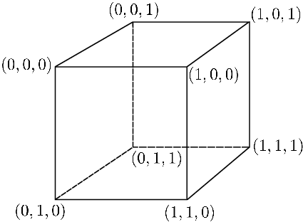
Figure 3: A 33-dimensional cube. A random walk on the cube is equivalent to a Markov chain ℳ\mathcal{M} with N=3N=3.

Finally, we simplify the notation of the Markov chain ℳ\mathcal{M}. Since it is equivalent to a Markov chain on a (N−1)(N-1)-dimensional hypercube with a transition matrix 𝒢\mathcal{G}, we label each vertex by a binary number i→=(i1,⋯,iN−1)∈{0,1}N−1\vec{i}=(i_{1},\cdots,i_{N-1})\in\{0,1\}^{N-1}, not by (𝐩,𝐪)(\mathbf{p},\mathbf{q}). If we identify (𝐩0,𝐪0)(\mathbf{p}_{0},\mathbf{q}_{0}) with i0→=0⋯0\vec{i_{0}}=0\cdots 0, a new label for fk​(𝐩0,𝐪0)f_{k}(\mathbf{p}_{0},\mathbf{q}_{0}) is given by 0⋯010⋯00\cdots 0{1}0\cdots 0 where only the kk-th digit of the binary representation is 11. The vertices i→\vec{i} and j→\vec{j} are connected if and only if H⁡(i→,j→)=1H(\vec{i},\vec{j})=1 where H⁡(i→,j→)=∑k|ik−jk|H(\vec{i},\vec{j})=\sum_{k}|i_{k}-j_{k}| (see Fig. 3). In this new labeling, the transition matrix 𝒢⁡[(𝐩,𝐪);(𝐩′,𝐪′)]\mathcal{G}[(\mathbf{p},\mathbf{q});(\mathbf{p}^{\prime},\mathbf{q}^{\prime})] is simplified to

𝒫⁡(i→,j→)={1−2N if ​i→=j→,2N⁡(N−1) if ​H​(i→,j→)=1,0 otherwise.\mathcal{P}(\vec{i},\vec{j})=\begin{cases}1-\frac{2}{N}&\text{ if }\vec{i}=\vec{j},\\ \frac{2}{N(N-1)}&\text{ if }H(\vec{i},\vec{j})=1,\\ 0&\text{ otherwise}.\end{cases} (19)

6.2.2 Lower bound on the mixing time of a Markov chain ℳ\mathcal{M}

The Markov chain on a (N−1)(N-1)-dimensional hypercube with a staying probability 1/21/2 has been well studied. For such a Markov chain, the transition matrix is given by I/2+𝒫′/2I/2+\mathcal{P}^{\prime}/2 where 𝒫′\mathcal{P}^{\prime} has a matrix element 1N−1\frac{1}{N-1} for H⁡(i→,j→)=1H(\vec{i},\vec{j})=1, and 00 otherwise. All eigenvalues of the transition matrix are known to be {1−kN−1}k=0,⋯,N−1\{1-\frac{k}{N-1}\}_{k=0,\cdots,N-1}[59]. On the other hand, it is observed from Eq. (19) that 𝒫⁡(i→,j→)=(1−2N)​I+2N​𝒫′\mathcal{P}(\vec{i},\vec{j})=(1-\frac{2}{N})I+\frac{2}{N}\mathcal{P}^{\prime}. Hence, the eigenvalues of 𝒫⁡(i→,j→)\mathcal{P}(\vec{i},\vec{j}) are given by {1−4​kN⁡(N−1)}k=0,⋯,N−1\{1-\frac{4k}{N(N-1)}\}_{k=0,\cdots,N-1}, which leads to maxi=2,3,⋯⁡|λi|=1−4N⁡(N−1)\max_{i=2,3,\cdots}|\lambda_{i}|=1-\frac{4}{N(N-1)}. Using Eq. (34) in E, the mixing time Tmix​(ϵ′)T_{\rm mix}(\epsilon^{\prime}) is bounded from below by

(N⁡(N−1)4−1)​log⁡12​ϵ′≤Tmix​(ϵ′).(\frac{N(N-1)}{4}-1)\log\frac{1}{2\epsilon^{\prime}}\leq T_{\rm mix}(\epsilon^{\prime}).

6.2.3 Upper bound of the mixing time of a Markov chain ℳ\mathcal{M}

In order to derive an upper bound on the mixing time, we slightly modify the transition matrix 𝒫⁡(i→,j→)\mathcal{P}(\vec{i},\vec{j}) by changing the staying probability from 1−2N1-\frac{2}{N} to 1−1N−11-\frac{1}{N-1}. A new transition matrix 𝒫~​(i→,j→)\tilde{\mathcal{P}}(\vec{i},\vec{j}) is given by

𝒫~​(i→,j→)={1−1N−1 if ​i→=j→,1(N−1)2 if ​H​(i→,j→)=1,0 otherwise.\tilde{\mathcal{P}}(\vec{i},\vec{j})=\begin{cases}1-\frac{1}{N-1}&\text{ if }\vec{i}=\vec{j},\\ \frac{1}{(N-1)^{2}}&\text{ if }H(\vec{i},\vec{j})=1,\\ 0&\text{ otherwise}.\end{cases}

We denote by ℳ~\tilde{\mathcal{M}} a new Markov chain with a transition matrix 𝒫~\tilde{\mathcal{P}}. Since the staying probability of 𝒫\mathcal{P} is smaller than 𝒫~\tilde{\mathcal{P}}, the mixing time of ℳ~\tilde{\mathcal{M}} provides an upper bound on that of ℳ\mathcal{M}.

We investigate the mixing time of the Markov chain ℳ~\tilde{\mathcal{M}} by the coupling method (see E). For constructing a coupling, we interpret ℳ~\tilde{\mathcal{M}} as follows. At a step t=k0+m⁡(N−1)t=k_{0}+m(N-1) (k0=1,⋯,N−1k_{0}=1,\cdots,N-1 and m=0,1,⋯m=0,1,\cdots), choose j∈{i1,⋯,iN−1}j\in\{i_{1},\cdots,i_{N-1}\} at random and, if j=ik0j=i_{k_{0}}, flip ik0i_{k_{0}}, otherwise, do nothing. Based on this, we define a coupling (Xk,Yk)(X_{k},Y_{k}). A state in XkX_{k} (YkY_{k}) is a bit sequence x1⋯xN−1x_{1}\cdots x_{N-1} (y1⋯yN−1y_{1}\cdots y_{N-1}) where xjx_{j} (yjy_{j}) ∈{0,1}\in\{0,1\}. At a step t=k0+m⁡(N−1)t=k_{0}+m(N-1) (k0=1,⋯,N−1k_{0}=1,\cdots,N-1 and m=0,1,⋯m=0,1,\cdots), we randomly choose j∈{i1,⋯,iN−1}j\in\{i_{1},\cdots,i_{N-1}\}. If j≠ik0j\neq i_{k_{0}}, do nothing. If j=ik0j=i_{k_{0}} and xj=yjx_{j}=y_{j}, flip both of them. If j=ik0j=i_{k_{0}} and xj≠yjx_{j}\neq y_{j}, flip xjx_{j} and yα⁡(j)y_{\alpha(j)} where α⁡(j)\alpha(j) is the position satisfying xα⁡(j)≠yα⁡(j)x_{\alpha(j)}\neq y_{\alpha(j)} next to jj. For instance, when X=(0,1,0,1,1)X=(0,1,0,1,1) and Y=(1,1,0,0,0)Y=(1,1,0,0,0), α⁡(1)=4\alpha(1)=4 and α⁡(4)=5\alpha(4)=5. Each of XkX_{k} and YkY_{k} is equivalent to the Markov chain ℳ~\tilde{\mathcal{M}} and they also satisfy Xk+1=Yk+1X_{k+1}=Y_{k+1} if Xk=YkX_{k}=Y_{k}. Hence, (Xk,Yk)(X_{k},Y_{k}) is a coupling of ℳ~\tilde{\mathcal{M}}.

To investigate the coupling, we use the property of a special type of Markov chain, a coupon collecting. A coupon collecting of rr-coupons is a Markov chain on a set of states {0,1,⋯,r}\{0,1,\cdots,r\} with transition matrix given by

Prob⁡[Xt+1=k+1|Xt=k]\displaystyle{\rm Prob}[X_{t+1}=k+1|X_{t}=k] =r−kr,\displaystyle=\frac{r-k}{r},
Prob⁡[Xt+1=k|Xt=k]\displaystyle{\rm Prob}[X_{t+1}=k|X_{t}=k] =kr.\displaystyle=\frac{k}{r}.

A coupon collecting of rr coupons is interpreted as a trial of collecting a complete set of rr different coupons by drawing one coupon at each step. When r0r_{0} coupons are initially at hand, we denote the necessary number of steps to draw all coupons by τcoupon(r,r0)\tau_{\rm coupon}^{(r,r_{0})}.

Proposition 5

Let (Xk,Yk)(X_{k},Y_{k}) be a coupling of ℳ~\tilde{\mathcal{M}} defined above and Tx​yT_{xy} be its stopping time. Then Tx​yT_{xy} is bounded from above by

Tx​y≤(N−1)​τcoupon(N−1,N−2).T_{xy}\leq(N-1)\tau_{\rm coupon}^{(N-1,N-2)}. (20)
Proof

By definition of the coupling, for a fixed k0∈{1,⋯,N−1}k_{0}\in\{1,\cdots,N-1\}, once ik0i_{k_{0}} is chosen at the steps k=k0+m⁡(N−1)k=k_{0}+m(N-1) (m=0,1,⋯m=0,1,\cdots), we have xik0=yik0x_{i_{k_{0}}}=y_{i_{k_{0}}}. The number of steps necessary for picking up k0k_{0} from {1,⋯,N−1}\{1,\cdots,N-1\} is equal to that of a coupon collecting of (N−1)(N-1)-coupons with initially N−2N-2 coupons at hand, that is, τcoupon(N−1,N−2)\tau_{\rm coupon}^{(N-1,N-2)}. Since there exists N−1N-1 choices of k0k_{0}, the stopping time Tx​yT_{xy} is smaller than or equal to (N−1)​τcoupon(N−1,N−2)(N-1)\tau_{\rm coupon}^{(N-1,N-2)}.

■\blacksquare

A coupon collecting of rr-coupons starting with no coupon is a well-studied problem. If we draw coupons r​log⁡rr\log r times, we can collect all rr coupons with high probability, that is, τcoupon(r,0)\tau_{\rm coupon}^{(r,0)} is typically given by r​log⁡rr\log r. For τcoupon(r,r0)\tau_{\rm coupon}^{(r,r_{0})}, we first show that

Prob[τcoupon(r,r0)>r(log(r−r0)+c)]≤e−c,{\rm Prob}[\tau_{\rm coupon}^{(r,r_{0})}>r(\log(r-r_{0})+c)]\leq e^{-c}, (21)

for any c>0c>0. This is shown in a standard way (see F for details).

By appealing to Theorem 4, Proposition 5 and Eq. (21), we can bound Δ⁡((N−1)2​c)\Delta((N-1)^{2}c) by

Δ⁡((N−1)2​c)\displaystyle\Delta((N-1)^{2}c) ≤maxx,yProb[Tx​y>(N−1)2c)]\displaystyle\leq\max_{x,y}{\rm Prob}[T_{xy}>(N-1)^{2}c)]
≤Prob[(N−1)τcoupon(N−1,N−2)>(N−1)2c]\displaystyle\leq{\rm Prob}[(N-1)\tau_{\rm coupon}^{(N-1,N-2)}>(N-1)^{2}c]
=Prob[τcoupon(N−1,N−2)>(N−1)c]\displaystyle={\rm Prob}[\tau_{\rm coupon}^{(N-1,N-2)}>(N-1)c]
<e−c.\displaystyle<e^{-c}.

Denote by T~mix​(ϵ′)\tilde{T}_{\rm mix}(\epsilon^{\prime}) the mixing time of the Markov chain ℳ~\tilde{\mathcal{M}} with an error ϵ′\epsilon^{\prime}. Since T~mix​(ϵ′)\tilde{T}_{\rm mix}(\epsilon^{\prime}) is defined by Δ⁡(T~mix​(ϵ′))≤ϵ′\Delta(\tilde{T}_{\rm mix}(\epsilon^{\prime}))\leq\epsilon^{\prime}, we obtain

T~mix​(ϵ′)≤(N−1)2​log⁡ϵ′−1,\tilde{T}_{\rm mix}(\epsilon^{\prime})\leq(N-1)^{2}\log\epsilon^{\prime-1},

which also provides an upper bound on the mixing time of the Markov chain ℳ\mathcal{M} since Tmix​(ϵ′)<T~mix​(ϵ′)T_{\rm mix}(\epsilon^{\prime})<\tilde{T}_{\rm mix}(\epsilon^{\prime}).

6.2.4 Upper and lower bounds of the convergence time Tconv​(ϵ)T_{\rm conv}(\epsilon)

We require an error ϵ/(Πsum​27​N)\epsilon/(\Pi_{\rm sum}2^{7N}) in order to obtain an upper bound on the convergence time Tconv​(ϵ)T_{\rm conv}(\epsilon) (see Eq. (16)) and, an error ϵ/Πsum\epsilon/\Pi_{\rm sum} for a lower bound (see Eq. (17)). Recalling that the unitary operation W~\tilde{W} consists of TW~=⌈N/2⌉T_{\tilde{W}}=\lceil N/2\rceil two-qubit gates, we obtain bounds for Tconv​(ϵ)T_{\rm conv}(\epsilon) such that

(N⁡(N−1)4−1)​log⁡(Πsum​(L(±),R(±))2​ϵ)≤Tconv​(ϵ)−TW~≤(N−1)2​log⁡(27​N​Πsum​(L(±),R(±))ϵ).(\frac{N(N-1)}{4}-1)\log(\frac{\Pi_{\rm sum}(L^{(\pm)},R^{(\pm)})}{2\epsilon})\leq T_{\rm conv}(\epsilon)-T_{\tilde{W}}\\ \leq(N-1)^{2}\log(\frac{2^{7N}\Pi_{\rm sum}(L^{(\pm)},R^{(\pm)})}{\epsilon}).

It is straightforward to show that Πsum​(L(±),R(±))≤1\Pi_{\rm sum}(L^{(\pm)},R^{(\pm)})\leq 1 for any (L(±),R(±))(L^{(\pm)},R^{(\pm)}) and any ρ0\rho_{0}. For the lower bound, there exist ρ0\rho_{0} and (L(±),R(±))(L^{(\pm)},R^{(\pm)}) such that Πsum​(L(±),R(±))=1\Pi_{\rm sum}(L^{(\pm)},R^{(\pm)})=1. Therefore, we finally obtain

N2+(N24+O⁡(N))​log​(2​ϵ)−1≤Tconv​(ϵ)≤7​N3​log​2+N2​log​ϵ−1+O⁡(N2),\frac{N}{2}+\biggl(\frac{N^{2}}{4}+O(N)\biggr)\log(2\epsilon)^{-1}\leq T_{\rm conv}(\epsilon)\leq 7N^{3}\log 2+N^{2}\log\epsilon^{-1}+O(N^{2}),

for any initial state ρ0\rho_{0}. This concludes the proof of Theorem 2.

7 Summary and concluding remarks

In this paper, we have introduced concepts of diagonal-unitary tt-designs and toric tt-designs that simulate up to the tt-th order of statistical moments of diagonal-unitary matrices and phase-random states, respectively. We have presented how to implement diagonal-unitary 22-designs with the computational basis for NN-qubit systems by using two types of the phase-random circuits, the CP and CZ phase-random circuit. We have shown that the CP phase-random circuit exactly achieves a diagonal-unitary 22-design after applying two-qubit diagonal gates on all pairs of qubits, which requires N⁡(N−1)/2N(N-1)/2 gates. On the other hand, the CZ phase-random circuit approximately achieves a diagonal-unitary 22-design after applying at most O⁡(N2​(N+log⁡1/ϵ))O(N^{2}(N+\log 1/\epsilon)) two-qubit diagonal gates on randomly chosen pairs of qubits. Due to the random choice of pairs, the number of gates exceeds N⁡(N−1)/2N(N-1)/2 despite the commutativity of gates. Our results show that random variables in the genuine two-qubit diagonal gate provide a stronger ability for randomizing phases. We have also presented a protocol generating an exact complex-projective 22-design by using the CP phase-random circuit, which is more feasible to implement in experiments comparing to previously known protocols.

In analogy with random circuits, which are shown to approximately achieve unitary tt-designs for any tt by applying p​o​l​y​(N,t)poly(N,t) two-qubit gates[30], it is natural to expect that the phase-random circuits with appropriate gate sets would also achieve diagonal-unitary tt-designs in p​o​l​y​(N,t)poly(N,t) iterations. However, this is not the case as long as we use two-qubit diagonal gates since there is a lack of the number of parameters due to the commutativity of gates. Thus, the gate set should include multi-qubit gates if only diagonal gates are used for constructing diagonal-unitary tt-designs for large tt. It is interesting to specify the diagonal gate set of the phase-random circuit achieving diagonal-unitary tt-designs for arbitrary tt and to construct a quantum circuit composed of non-diagonal two-qubit gates that achieves diagonal-unitary tt-designs, which will be addressed in a separate paper[61].

Acknowledgment

The authors thank F. G. S. L. Brandao for insightful comments on unitary tt-designs, M. Koashi for important suggestions for the CP phase-random circuit, and P. S. Turner for helpful discussions. This work was supported by Project for Developing Innovation Systems of the Ministry of Education, Culture, Sports, Science and Technology (MEXT), Japan. Y. N. acknowledges support from JSPS by KAKENHI (Grant No. 222812) and M. M. acknowledges support from JSPS by KAKENHI (Grant No. 23540463).

Appendix A Discrete phases are sufficient to achieve diagonal-unitary tt-designs

We show that a set of unitary matrices Ωt={∑nei​ϕn|un⟩⟨un|}\Omega_{t}=\{\sum_{n}e^{i\phi_{n}}\left|u_{n}\rangle\langle u_{n}\right|\}, where ϕn\phi_{n} is randomly chosen from {2​π​kt+1}k=0,1,⋯,t\{\frac{2\pi k}{t+1}\}_{k=0,1,\cdots,t}, is a diagonal-unitary tt-design in the basis {|un⟩}\{\left|u_{n}\right\rangle\}.

For Uϕ=∑nei​ϕn|un⟩⟨un|U_{\phi}=\sum_{n}e^{i\phi_{n}}\left|u_{n}\rangle\langle u_{n}\right|, Uϕ⊗t⊗Uϕ†⊗tU_{\phi}^{\otimes t}\otimes U_{\phi}^{{\dagger}\otimes t} is calculated to

Uϕ⊗t⊗Uϕ†⊗t=∑nk,mkexp[i∑k=1t(ϕnk−ϕmk)]|un1⋯untum1⋯umt⟩⟨un1⋯untum1⋯umt|,U_{\phi}^{\otimes t}\otimes U_{\phi}^{{\dagger}\otimes t}=\sum_{n_{k},m_{k}}\exp[i\sum_{k=1}^{t}(\phi_{n_{k}}-\phi_{m_{k}})]\left|u_{n_{1}}\cdots u_{n_{t}}u_{m_{1}}\cdots u_{m_{t}}\rangle\langle u_{n_{1}}\cdots u_{n_{t}}u_{m_{1}}\cdots u_{m_{t}}\right|,

where the summations are taken over n1,⋯,nt=1,⋯,dn_{1},\cdots,n_{t}=1,\cdots,d and m1,⋯,mt=1,⋯,dm_{1},\cdots,m_{t}=1,\cdots,d.

For 𝒰diag(t)\mathcal{U}_{\rm diag}^{(t)} and Ωt\Omega_{t}, the expectation of an operator XX is taken over ϕi∈[0,2​π)\phi_{i}\in[0,2\pi) and ϕi′∈{2​π​kt+1}k=0,1,⋯,t\phi_{i}^{\prime}\in\{\frac{2\pi k}{t+1}\}_{k=0,1,\cdots,t} for all i=1,⋯,di=1,\cdots,d, respectively, namely,

𝔼𝒰diag(t)[X]=1(2​π)d∫02​πXdϕ1⋯dϕd,\displaystyle\mathbb{E}_{\mathcal{U}_{\rm diag}^{(t)}}[X]=\frac{1}{(2\pi)^{d}}\int_{0}^{2\pi}Xd\phi_{1}\cdots d\phi_{d},
𝔼Ωt[X]=(1t+1)d∑ϕ1′=0,⋯,2​π​tt+1⋯∑ϕd′=0,⋯,2​π​tt+1X.\displaystyle\mathbb{E}_{\Omega_{t}}[X]=(\frac{1}{t+1})^{d}\sum_{\phi_{1}^{\prime}=0,\cdots,\frac{2\pi t}{t+1}}\cdots\sum_{\phi_{d}^{\prime}=0,\cdots,\frac{2\pi t}{t+1}}X.

The equation 𝔼Ωt[U⊗t⊗U†⊗t]=𝔼𝒰diag(t)[U⊗t⊗U†⊗t]\mathbb{E}_{\Omega_{t}}[U^{\otimes t}\otimes U^{{\dagger}\otimes t}]=\mathbb{E}_{\mathcal{U}_{\rm diag}^{(t)}}[U^{\otimes t}\otimes U^{{\dagger}\otimes t}] follows from an identity that

1(2​π)d∫02​πexp[i∑k=1t(ϕnk−ϕmk)]dϕ1⋯dϕd=(1t+1)d∑ϕ1′=0,⋯,2​π​tt+1⋯∑ϕd′=0,⋯,2​π​tt+1exp[i∑k=1t(ϕnk′−ϕmk′)].\frac{1}{(2\pi)^{d}}\int_{0}^{2\pi}\exp[i\sum_{k=1}^{t}(\phi_{n_{k}}-\phi_{m_{k}})]d\phi_{1}\cdots d\phi_{d}=\\ (\frac{1}{t+1})^{d}\sum_{\phi_{1}^{\prime}=0,\cdots,\frac{2\pi t}{t+1}}\cdots\sum_{\phi_{d}^{\prime}=0,\cdots,\frac{2\pi t}{t+1}}\exp[i\sum_{k=1}^{t}(\phi_{n_{k}}^{\prime}-\phi_{m_{k}}^{\prime})]. (22)

Thus, discrete phases are sufficient to achieve a diagonal-unitary tt-design.

Appendix B Discrete phases in the C​PCP phase-random circuits

We show that, in the CP phase-random circuits, it is sufficient to choose the phases α\alpha and β\beta from {0,2​π3,4​π3}\{0,\frac{2\pi}{3},\frac{4\pi}{3}\}, and γ\gamma from {0,π}\{0,\pi\}, instead of choosing the phases uniformly from [0,2​π)[0,2\pi).

To show this, we consider two expectations of W:=(∏i<jWi​j​(αi​j,βi​j,γi​j))⊗2⊗(∏i<jWi​j†​(αi​j,βi​j,γi​j))⊗2W:=(\prod_{i<j}W_{ij}(\alpha_{ij},\beta_{ij},\gamma_{ij}))^{\otimes 2}\otimes(\prod_{i<j}W_{ij}^{\dagger}(\alpha_{ij},\beta_{ij},\gamma_{ij}))^{\otimes 2}, where Wi​j​(αi​j,βi​j,γi​j)∈𝒲diagC​PW_{ij}(\alpha_{ij},\beta_{ij},\gamma_{ij})\in\mathcal{W}_{\rm diag}^{CP} acts on the iith and jjth qubits with phases αi​j,βi​j,γi​j\alpha_{ij},\beta_{ij},\gamma_{ij}. One expectation is taken over α,β,γ∈[0,2​π)\alpha,\beta,\gamma\in[0,2\pi) and is denoted by 𝔼cont​[W]\mathbb{E}_{\rm cont}[W]. The other is taken over α,β∈{0,2​π3,4​π3}\alpha,\beta\in\{0,\frac{2\pi}{3},\frac{4\pi}{3}\} and γ∈{0,π}\gamma\in\{0,\pi\} and is denoted by 𝔼disc​[W]\mathbb{E}_{\rm disc}[W]. Due to the fact that all αi​j,βi​j\alpha_{ij},\beta_{ij} and γi​j\gamma_{ij} are independent, both expectations are given by

𝔼⁡[W]=∏i<j𝔼⁡[Wi​j​(αi​j,βi​j,γi​j)⊗2⊗Wi​j†​(αi​j,βi​j,γi​j)⊗2].\mathbb{E}[W]=\prod_{i<j}\mathbb{E}[W_{ij}(\alpha_{ij},\beta_{ij},\gamma_{ij})^{\otimes 2}\otimes W_{ij}^{\dagger}(\alpha_{ij},\beta_{ij},\gamma_{ij})^{\otimes 2}].

In Wi​j​(αi​j,βi​j,γi​j)⊗2⊗Wi​j†​(αi​j,βi​j,γi​j)⊗2W_{ij}(\alpha_{ij},\beta_{ij},\gamma_{ij})^{\otimes 2}\otimes W_{ij}^{\dagger}(\alpha_{ij},\beta_{ij},\gamma_{ij})^{\otimes 2}, all terms except those equal to 11, e.g., ei​αi​je^{i\alpha_{ij}}, ei​βi​je^{i\beta_{ij}}, ei​2​αi​je^{i2\alpha_{ij}} and ei⁡(αi​j+βi​j+γi​j)e^{i(\alpha_{ij}+\beta_{ij}+\gamma_{ij})}, disappear by integrating over αi​j,βi​j\alpha_{ij},\beta_{ij} and γi​j\gamma_{ij}. This is the case even if we average over αi​j,βi​j∈{0,2​π3,4​π3}\alpha_{ij},\beta_{ij}\in\{0,\frac{2\pi}{3},\frac{4\pi}{3}\} and γi​j∈{0,π}\gamma_{ij}\in\{0,\pi\}, since Wi​j⊗2​(αi​j,βi​j,γi​j)⊗Wi​j†​(αi​j,βi​j,γi​j)⊗2W_{ij}^{\otimes 2}(\alpha_{ij},\beta_{ij},\gamma_{ij})\otimes W_{ij}^{\dagger}(\alpha_{ij},\beta_{ij},\gamma_{ij})^{\otimes 2} does not contain terms such as e3​i​αi​je^{3i\alpha_{ij}}, e3​i​βi​je^{3i\beta_{ij}} and e2​i​γe^{2i\gamma}. Thus, it is shown that 𝔼cont​[W]=𝔼disc​[W]\mathbb{E}_{\rm cont}[W]=\mathbb{E}_{\rm disc}[W], namely, αi​j,βi​j\alpha_{ij},\beta_{ij} can be chosen from {0,2​π3,4​π3}\{0,\frac{2\pi}{3},\frac{4\pi}{3}\} and γi​j\gamma_{ij} from {0,π}\{0,\pi\}.

Appendix C Necessary and sufficient conditions for an ϵ\epsilon-approximate diagonal-unitary 22-design in terms of the expansion coefficients

An ϵ\epsilon-approximate diagonal-unitary 22-design 𝒰diag(2,ϵ)\mathcal{U}^{(2,\epsilon)}_{\rm diag} is defined by

‖ℰ𝒰diag(2,ϵ)(2)−ℰ𝒰diag(2)‖⋄≤ϵ,|\!|\mathcal{E}^{(2)}_{\mathcal{U}^{(2,\epsilon)}_{\rm diag}}-\mathcal{E}^{(2)}_{\mathcal{U}_{\rm diag}}|\!|_{\diamond}\leq\epsilon, (23)

where 𝒰diag\mathcal{U}_{\rm diag} is random diagonal-unitary matrices and ℰ𝒱(2)\mathcal{E}^{(2)}_{\mathcal{V}} for an ensemble of unitary matrices 𝒱\mathcal{V} is a superoperator defined by Eq. (1). We show that sufficient and necessary conditions for Eq. (23) to hold in terms of 𝔼CTC​Z​[ξT​(𝐩,𝐪)]\mathbb{E}_{C_{T}^{CZ}}[\xi_{T}(\mathbf{p},\mathbf{q})] are given by

∀(𝐩,𝐪),|𝔼CTC​Z​[ξT​(𝐩,𝐪)]−𝔼C∞C​Z​[ξ∞​(𝐩,𝐪)]|≤ϵ27​N,\forall(\mathbf{p},\mathbf{q}),\biggl|\mathbb{E}_{C_{T}^{CZ}}[\xi_{T}(\mathbf{p},\mathbf{q})]-\mathbb{E}_{C_{\infty}^{CZ}}[\xi_{\infty}(\mathbf{p},\mathbf{q})]\biggr|\leq\frac{\epsilon}{2^{7N}}, (24)

and

∀(𝐩,𝐪),|𝔼CTC​Z​[ξT​(𝐩,𝐪)]−𝔼C∞C​Z​[ξ∞​(𝐩,𝐪)]|≤ϵ,\forall(\mathbf{p},\mathbf{q}),\biggl|\mathbb{E}_{C_{T}^{CZ}}[\xi_{T}(\mathbf{p},\mathbf{q})]-\mathbb{E}_{C_{\infty}^{CZ}}[\xi_{\infty}(\mathbf{p},\mathbf{q})]\biggr|\leq\epsilon, (25)

respectively, for any initial state ρ0\rho_{0} on a 2​N2N-qubit system.

First, we assume Eq. (24). It implies

∀ρ0,∑(𝐩,𝐪)|𝔼CTC​Z​[ξT​(𝐩,𝐪)]−𝔼C∞C​Z​[ξ∞​(𝐩,𝐪)]|≤ϵ23​N\displaystyle\forall\rho_{0},\sum_{(\mathbf{p},\mathbf{q})}\biggl|\mathbb{E}_{C_{T}^{CZ}}[\xi_{T}(\mathbf{p},\mathbf{q})]-\mathbb{E}_{C_{\infty}^{CZ}}[\xi_{\infty}(\mathbf{p},\mathbf{q})]\biggr|\leq\frac{\epsilon}{2^{3N}} (26)
⇒∀ρ0,||∑(𝐩,𝐪)(𝔼CTC​Z[ξT(𝐩,𝐪)]−𝔼C∞C​Z[ξ∞(𝐩,𝐪)])σ𝐩⊗σ𝐪||1≤ϵ2N\displaystyle\Rightarrow\forall\rho_{0},\biggl|\!\biggl|\sum_{(\mathbf{p},\mathbf{q})}\biggr(\mathbb{E}_{C_{T}^{CZ}}[\xi_{T}(\mathbf{p},\mathbf{q})]-\mathbb{E}_{C_{\infty}^{CZ}}[\xi_{\infty}(\mathbf{p},\mathbf{q})]\biggr)\sigma_{\mathbf{p}}\otimes\sigma_{\mathbf{q}}\biggr|\!\biggr|_{1}\leq\frac{\epsilon}{2^{N}} (27)
⇔∀ρ0,‖ℰ𝒰(2,ϵ)(2)​(ρ0)−ℰ𝒰(2)​(ρ0)‖1≤ϵ22​N\displaystyle\Leftrightarrow\forall\rho_{0},|\!|\mathcal{E}^{(2)}_{\mathcal{U}^{(2,\epsilon)}}(\rho_{0})-\mathcal{E}^{(2)}_{\mathcal{U}}(\rho_{0})|\!|_{1}\leq\frac{\epsilon}{2^{2N}} (28)
⇒‖ℰ𝒰(2,ϵ)(2)−ℰ𝒰(2)‖⋄≤ϵ,\displaystyle\Rightarrow|\!|\mathcal{E}^{(2)}_{\mathcal{U}^{(2,\epsilon)}}-\mathcal{E}^{(2)}_{\mathcal{U}}|\!|_{\diamond}\leq\epsilon, (29)

where the Cauchy-Schwarz inequality is used to obtained the first relation and, a relation that ∀ρ,‖ℰ⁡(ρ)‖1≤α\forall\rho,|\!|\mathcal{E}(\rho)|\!|_{1}\leq\alpha implies ‖ℰ‖⋄≤d​α|\!|\mathcal{E}|\!|_{\diamond}\leq d\alpha, where dd is a dimension of the space that ρ\rho acts on, is used to obtain the last relation. This provides the sufficient condition.

To obtain a necessary condition, we start from ‖ℰ𝒰(2,ϵ)(2)−ℰ𝒰(2)‖⋄≤ϵ|\!|\mathcal{E}^{(2)}_{\mathcal{U}^{(2,\epsilon)}}-\mathcal{E}^{(2)}_{\mathcal{U}}|\!|_{\diamond}\leq\epsilon and use a fact that ‖ℰ‖⋄≥‖ℰ⁡(ρ)‖1|\!|\mathcal{E}|\!|_{\diamond}\geq|\!|\mathcal{E}(\rho)|\!|_{1} for any state ρ\rho. In terms of the expansion coefficients, we obtain

∀ρ0,2−N||∑(𝐩,𝐪)(𝔼CTC​Z[ξT(𝐩,𝐪)]−𝔼C∞C​Z[ξ∞(𝐩,𝐪)])σ𝐩⊗σ𝐪||1≤ϵ\displaystyle\forall\rho_{0},2^{-N}\biggl|\!\biggl|\sum_{(\mathbf{p},\mathbf{q})}\biggr(\mathbb{E}_{C_{T}^{CZ}}[\xi_{T}(\mathbf{p},\mathbf{q})]-\mathbb{E}_{C_{\infty}^{CZ}}[\xi_{\infty}(\mathbf{p},\mathbf{q})]\biggr)\sigma_{\mathbf{p}}\otimes\sigma_{\mathbf{q}}\biggr|\!\biggr|_{1}\leq\epsilon (30)
⇒∀ρ0,2−N||∑(𝐩,𝐪)(𝔼CTC​Z[ξT(𝐩,𝐪)]−𝔼C∞C​Z[ξ∞(𝐩,𝐪)])σ𝐩⊗σ𝐪||2≤ϵ\displaystyle\Rightarrow\forall\rho_{0},2^{-N}\biggl|\!\biggl|\sum_{(\mathbf{p},\mathbf{q})}\biggr(\mathbb{E}_{C_{T}^{CZ}}[\xi_{T}(\mathbf{p},\mathbf{q})]-\mathbb{E}_{C_{\infty}^{CZ}}[\xi_{\infty}(\mathbf{p},\mathbf{q})]\biggr)\sigma_{\mathbf{p}}\otimes\sigma_{\mathbf{q}}\biggr|\!\biggr|_{2}\leq\epsilon (31)
⇔∀ρ0,∑(𝐩,𝐪)(𝔼CTC​Z​[ξT​(𝐩,𝐪)]−𝔼C∞C​Z​[ξ∞​(𝐩,𝐪)])2≤ϵ2\displaystyle\Leftrightarrow\forall\rho_{0},\sum_{(\mathbf{p},\mathbf{q})}\biggl(\mathbb{E}_{C_{T}^{CZ}}[\xi_{T}(\mathbf{p},\mathbf{q})]-\mathbb{E}_{C_{\infty}^{CZ}}[\xi_{\infty}(\mathbf{p},\mathbf{q})]\biggr)^{2}\leq\epsilon^{2} (32)
⇒∀ρ0,∀(𝐩,𝐪),|𝔼CTC​Z​[ξT​(𝐩,𝐪)]−𝔼C∞C​Z​[ξ∞​(𝐩,𝐪)]|≤ϵ,\displaystyle\Rightarrow\forall\rho_{0},\forall(\mathbf{p},\mathbf{q}),\biggl|\mathbb{E}_{C_{T}^{CZ}}[\xi_{T}(\mathbf{p},\mathbf{q})]-\mathbb{E}_{C_{\infty}^{CZ}}[\xi_{\infty}(\mathbf{p},\mathbf{q})]\biggr|\leq\epsilon, (33)

where ‖X‖2=Tr​X†​X|\!|X|\!|_{2}=\sqrt{\mathrm{Tr}X^{\dagger}X} is a Hilbert-Schmidt norm. Thus we obtain the necessary condition.

Appendix D Calculation of Gi​j​(𝐩,𝐪,𝐩′,𝐪′)G_{ij}(\mathbf{p},\mathbf{q};\mathbf{p}^{\prime},\mathbf{q}^{\prime})

Gi​j​(𝐩,𝐪,𝐩′,𝐪′)G_{ij}(\mathbf{p},\mathbf{q};\mathbf{p}^{\prime},\mathbf{q}^{\prime}) is defined by

Gi​j​(𝐩,𝐪,𝐩′,𝐪′)=𝔼⁡[Tr​σ𝐩​Wi​j​σ𝐩′​Wi​j†​Tr​σ𝐪​Wi​j​σ𝐪′​Wi​j†],G_{ij}(\mathbf{p},\mathbf{q};\mathbf{p}^{\prime},\mathbf{q}^{\prime})=\mathbb{E}[\mathrm{Tr}\sigma_{\mathbf{p}}W_{ij}\sigma_{\mathbf{p}^{\prime}}W_{ij}^{\dagger}\mathrm{Tr}\sigma_{\mathbf{q}}W_{ij}\sigma_{\mathbf{q}^{\prime}}W_{ij}^{\dagger}],

where Wi​jW_{ij} is a two-qubit diagonal gate on the ii-th and jj-th qubits and randomly chosen from the gate set 𝒲C​Z={d​i​a​g​(1,ei​α,ei​β,−ei⁡(α+β))}α,β\mathcal{W}^{CZ}=\{diag(1,e^{i\alpha},e^{i\beta},-e^{i(\alpha+\beta)})\}_{\alpha,\beta} or 𝒲C​P={d​i​a​g​(1,ei​α,ei​β,ei​γ)}α,β,γ\mathcal{W}^{CP}=\{diag(1,e^{i\alpha},e^{i\beta},e^{i\gamma})\}_{\alpha,\beta,\gamma}. Since 𝒲C​P\mathcal{W}^{CP} is more general than 𝒲C​Z\mathcal{W}^{CZ}, we start with the calculation of Gi​j​(𝐩,𝐪,𝐩′,𝐪′)G_{ij}(\mathbf{p},\mathbf{q};\mathbf{p}^{\prime},\mathbf{q}^{\prime}) for 𝒲C​P\mathcal{W}^{CP}.

In order to calculate Gi​j​(𝐩,𝐪,𝐩′,𝐪′)G_{ij}(\mathbf{p},\mathbf{q};\mathbf{p}^{\prime},\mathbf{q}^{\prime}), we define 𝒟a​b,ℰa​b\mathcal{D}_{ab},\mathcal{E}_{ab} and Δa\Delta_{a} by

𝒟a​b\displaystyle\mathcal{D}_{ab} =δa​0​δb​z+δa​z​δb​0,\displaystyle=\delta_{a0}\delta_{bz}+\delta_{az}\delta_{b0},
ℰa​b\displaystyle\mathcal{E}_{ab} =δa​x​δb​y−δa​y​δb​x,\displaystyle=\delta_{ax}\delta_{by}-\delta_{ay}\delta_{bx},

and

Δa=δa​0+δa​z−δa​x−δa​y.\Delta_{a}=\delta_{a0}+\delta_{az}-\delta_{ax}-\delta_{ay}.

We also use a notation that δn∈S=1\delta_{n\in S}=1 if n∈Sn\in S and δn∈S=0\delta_{n\in S}=0 if n∉Sn\notin S.

For Wi​j=d​i​a​g​(1,ei​α,ei​β,ei​γ)W_{ij}=diag(1,e^{i\alpha},e^{i\beta},e^{i\gamma}), it is straightforward to calculate Tr​σ𝐩​Wi​j​σ𝐩′​Wi​j†\mathrm{Tr}\sigma_{\mathbf{p}}W_{ij}\sigma_{\mathbf{p}^{\prime}}W_{ij}^{\dagger} and we obtain

12N​Tr​σ𝐩​Wi​j​σ𝐩′​Wi​j†\displaystyle\frac{1}{2^{N}}\mathrm{Tr}\sigma_{\mathbf{p}}W_{ij}\sigma_{\mathbf{p}^{\prime}}W_{ij}^{\dagger}
=δ𝐩,𝐩′{δpi,pj∈{0,z}+12δpi∈{x,y}(cosβ+cos(α−γ))+12δpj∈{x,y}(cosα+cos(β−γ))\displaystyle=\delta_{\mathbf{p},\mathbf{p}^{\prime}}\biggl\{\delta_{p_{i},p_{j}\in\{0,z\}}+\frac{1}{2}\delta_{p_{i}\in\{x,y\}}\bigl(\cos\beta+\cos(\alpha-\gamma)\bigr)+\frac{1}{2}\delta_{p_{j}\in\{x,y\}}\bigl(\cos\alpha+\cos(\beta-\gamma)\bigr)
−12δpi,pj∈{x,y}[cosα+cosβ−cosγ−cos(α−β)+cos(α−γ)+cos(β−γ)]}\displaystyle\hskip 28.45274pt-\frac{1}{2}\delta_{p_{i},p_{j}\in\{x,y\}}\bigl[\cos\alpha+\cos\beta-\cos\gamma-\cos(\alpha-\beta)+\cos(\alpha-\gamma)+\cos(\beta-\gamma)\bigr]\biggr\}
+12δpi,pi′{δpi∈{x,y}(cosβ−cos(α−γ))𝒟pj,pj′\displaystyle+\frac{1}{2}\delta_{p_{i},p_{i}^{\prime}}\biggl\{\delta_{p_{i}\in\{x,y\}}\bigl(\cos\beta-\cos(\alpha-\gamma)\bigr)\mathcal{D}_{p_{j},p_{j}^{\prime}}
−[δpi∈{0,z}(sinα−sin(β−γ))+δpi∈{x,y}(sinγ+sin(α−β))]ℰpj,pj′}\displaystyle\hskip 28.45274pt-\bigl[\delta_{p_{i}\in\{0,z\}}\bigl(\sin\alpha-\sin(\beta-\gamma)\bigr)+\delta_{p_{i}\in\{x,y\}}\bigl(\sin\gamma+\sin(\alpha-\beta)\bigr)\bigr]\mathcal{E}_{p_{j},p_{j}^{\prime}}\biggr\}
+12δpj,pj′{δpj∈{x,y}(cosα−cos(β−γ))𝒟pi,pi′\displaystyle+\frac{1}{2}\delta_{p_{j},p_{j}^{\prime}}\biggl\{\delta_{p_{j}\in\{x,y\}}\bigl(\cos\alpha-\cos(\beta-\gamma)\bigr)\mathcal{D}_{p_{i},p_{i}^{\prime}}
−[δpj∈{0,z}(sinβ−sin(α−γ))+δpj∈{x,y}(sinγ+sin(β−α))]ℰpi,pi′}\displaystyle\hskip 28.45274pt-\bigl[\delta_{p_{j}\in\{0,z\}}\bigl(\sin\beta-\sin(\alpha-\gamma)\bigr)+\delta_{p_{j}\in\{x,y\}}\bigl(\sin\gamma+\sin(\beta-\alpha)\bigr)\bigr]\mathcal{E}_{p_{i},p_{i}^{\prime}}\biggr\}
−12​(sin⁡β+sin⁡(α−γ))​ℰpi,pi′​𝒟pj,pj′−12​(sin⁡α+sin⁡(β−γ))​𝒟pi,pi′​ℰpj,pj′\displaystyle-\frac{1}{2}\bigl(\sin\beta+\sin(\alpha-\gamma)\bigr)\mathcal{E}_{p_{i},p_{i}^{\prime}}\mathcal{D}_{p_{j},p_{j}^{\prime}}-\frac{1}{2}\bigl(\sin\alpha+\sin(\beta-\gamma)\bigr)\mathcal{D}_{p_{i},p_{i}^{\prime}}\mathcal{E}_{p_{j},p_{j}^{\prime}}
+12​(cos⁡(α−β)−cos⁡γ)​ℰpi,pi′​ℰpj,pj′.\displaystyle\hskip 28.45274pt+\frac{1}{2}\bigl(\cos(\alpha-\beta)-\cos\gamma\bigr)\mathcal{E}_{p_{i},p_{i}^{\prime}}\mathcal{E}_{p_{j},p_{j}^{\prime}}.

In the case of 𝒲C​P\mathcal{W}^{CP}, by taking the average over α,β=0,2​π3,4​π3\alpha,\beta=0,\frac{2\pi}{3},\frac{4\pi}{3} and γ=0,π\gamma=0,\pi, Gi​jG_{ij} is calculated to

122​N​Gi​j​(𝐩,𝐪,𝐩′,𝐪′)=\displaystyle\frac{1}{2^{2N}}G_{ij}(\mathbf{p},\mathbf{q};\mathbf{p}^{\prime},\mathbf{q}^{\prime})= δ𝐩,𝐩′​δ𝐪,𝐪′​(δpi,pj,qi,qj∈{0,z}+14​δpi,qi∈{0,z}​δpj,qj∈{x,y}CLOSE\displaystyle\delta_{\mathbf{p},\mathbf{p}^{\prime}}\delta_{\mathbf{q},\mathbf{q}^{\prime}}\biggl(\delta_{p_{i},p_{j},q_{i},q_{j}\in\{0,z\}}+\frac{1}{4}\delta_{p_{i},q_{i}\in\{0,z\}}\delta_{p_{j},q_{j}\in\{x,y\}}
OPEN+14​δpi,qi∈{x,y}​δpj,qj∈{0,z}+14​δpi,pj,qi,qj∈{x,y})\displaystyle+\frac{1}{4}\delta_{p_{i},q_{i}\in\{x,y\}}\delta_{p_{j},q_{j}\in\{0,z\}}+\frac{1}{4}\delta_{p_{i},p_{j},q_{i},q_{j}\in\{x,y\}}\biggr)
+14​δpi,qi∈{x,y}​δpi,pi′​δqi,qi′​(𝒟pj,pj′​𝒟qj,qj′+ℰpj,pj′​ℰqj,qj′)\displaystyle+\frac{1}{4}\delta_{p_{i},q_{i}\in\{x,y\}}\delta_{p_{i},p_{i}^{\prime}}\delta_{q_{i},q_{i}^{\prime}}\biggl(\mathcal{D}_{p_{j},p_{j}^{\prime}}\mathcal{D}_{q_{j},q_{j}^{\prime}}+\mathcal{E}_{p_{j},p_{j}^{\prime}}\mathcal{E}_{q_{j},q_{j}^{\prime}}\biggr)
+14​δpj,qj∈{x,y}​δpj,pj′​δqj,qj′​(𝒟pi,pi′​𝒟qi,qi′+ℰpi,pi′​ℰqi,qi′)\displaystyle+\frac{1}{4}\delta_{p_{j},q_{j}\in\{x,y\}}\delta_{p_{j},p_{j}^{\prime}}\delta_{q_{j},q_{j}^{\prime}}\biggl(\mathcal{D}_{p_{i},p_{i}^{\prime}}\mathcal{D}_{q_{i},q_{i}^{\prime}}+\mathcal{E}_{p_{i},p_{i}^{\prime}}\mathcal{E}_{q_{i},q_{i}^{\prime}}\biggr)
+14​ℰpi,pi′​ℰqi,qi′​(δpj,qj∈{0,z}​δpj,pj′​δqj,qj′+𝒟pj,pj′​𝒟qj,qj′)\displaystyle+\frac{1}{4}\mathcal{E}_{p_{i},p_{i}^{\prime}}\mathcal{E}_{q_{i},q_{i}^{\prime}}\biggl(\delta_{p_{j},q_{j}\in\{0,z\}}\delta_{p_{j},p_{j}^{\prime}}\delta_{q_{j},q_{j}^{\prime}}+\mathcal{D}_{p_{j},p_{j}^{\prime}}\mathcal{D}_{q_{j},q_{j}^{\prime}}\biggr)
+14​ℰpj,pj′​ℰqj,qj′​(δpi,qi∈{0,z}​δpi,pi′​δqi,qi′+𝒟pi,pi′​𝒟qi,qi′)\displaystyle+\frac{1}{4}\mathcal{E}_{p_{j},p_{j}^{\prime}}\mathcal{E}_{q_{j},q_{j}^{\prime}}\biggl(\delta_{p_{i},q_{i}\in\{0,z\}}\delta_{p_{i},p_{i}^{\prime}}\delta_{q_{i},q_{i}^{\prime}}+\mathcal{D}_{p_{i},p_{i}^{\prime}}\mathcal{D}_{q_{i},q_{i}^{\prime}}\biggr)
+14​ℰpi,pi′​ℰqi,qi′​ℰpj,pj′​ℰqj,qj′.\displaystyle+\frac{1}{4}\mathcal{E}_{p_{i},p_{i}^{\prime}}\mathcal{E}_{q_{i},q_{i}^{\prime}}\mathcal{E}_{p_{j},p_{j}^{\prime}}\mathcal{E}_{q_{j},q_{j}^{\prime}}.

By investigating each case, we obtain Eq. (7).

On the other hand, in the case of 𝒲C​Z\mathcal{W}^{CZ}, γ\gamma is set to be α+β+π\alpha+\beta+\pi and Gi​jG_{ij} is obtained as

122​N​Gi​j​(𝐩,𝐪,𝐩′,𝐪′)=\displaystyle\frac{1}{2^{2N}}G_{ij}(\mathbf{p},\mathbf{q};\mathbf{p}^{\prime},\mathbf{q}^{\prime})= δ𝐩,𝐩′​δ𝐪,𝐪′​(δpi,pj,qi,qj∈{0,z}+14​δpi,pj,qi,qj∈{x,y})\displaystyle\delta_{\mathbf{p},\mathbf{p}^{\prime}}\delta_{\mathbf{q},\mathbf{q}^{\prime}}\biggl(\delta_{p_{i},p_{j},q_{i},q_{j}\in\{0,z\}}+\frac{1}{4}\delta_{p_{i},p_{j},q_{i},q_{j}\in\{x,y\}}\biggr)
+12​δpi,qi∈{x,y}​δpi,pi′​δqi,qi′​(𝒟pj,pj′​𝒟qj,qj′+12​ℰpj,pj′​ℰqj,qj′)\displaystyle+\frac{1}{2}\delta_{p_{i},q_{i}\in\{x,y\}}\delta_{p_{i},p_{i}^{\prime}}\delta_{q_{i},q_{i}^{\prime}}\biggl(\mathcal{D}_{p_{j},p_{j}^{\prime}}\mathcal{D}_{q_{j},q_{j}^{\prime}}+\frac{1}{2}\mathcal{E}_{p_{j},p_{j}^{\prime}}\mathcal{E}_{q_{j},q_{j}^{\prime}}\biggr)
+12​δpj,qj∈{x,y}​δpj,pj′​δqj,qj′​(𝒟pi,pi′​𝒟qi,qi′+12​ℰpi,pi′​ℰqi,qi′)\displaystyle+\frac{1}{2}\delta_{p_{j},q_{j}\in\{x,y\}}\delta_{p_{j},p_{j}^{\prime}}\delta_{q_{j},q_{j}^{\prime}}\biggl(\mathcal{D}_{p_{i},p_{i}^{\prime}}\mathcal{D}_{q_{i},q_{i}^{\prime}}+\frac{1}{2}\mathcal{E}_{p_{i},p_{i}^{\prime}}\mathcal{E}_{q_{i},q_{i}^{\prime}}\biggr)
+12​𝒟pi,pi′​𝒟qi,qi′​ℰpj,pj′​ℰqj,qj′+12​ℰpi,pi′​ℰqi,qi′​𝒟pj,pj′​𝒟qj,qj′\displaystyle+\frac{1}{2}\mathcal{D}_{p_{i},p_{i}^{\prime}}\mathcal{D}_{q_{i},q_{i}^{\prime}}\mathcal{E}_{p_{j},p_{j}^{\prime}}\mathcal{E}_{q_{j},q_{j}^{\prime}}+\frac{1}{2}\mathcal{E}_{p_{i},p_{i}^{\prime}}\mathcal{E}_{q_{i},q_{i}^{\prime}}\mathcal{D}_{p_{j},p_{j}^{\prime}}\mathcal{D}_{q_{j},q_{j}^{\prime}}
+14​ℰpi,pi′​ℰqi,qi′​ℰpj,pj′​ℰqj,qj′\displaystyle+\frac{1}{4}\mathcal{E}_{p_{i},p_{i}^{\prime}}\mathcal{E}_{q_{i},q_{i}^{\prime}}\mathcal{E}_{p_{j},p_{j}^{\prime}}\mathcal{E}_{q_{j},q_{j}^{\prime}}

leading to Eq. (9).

Appendix E Introduction of Markov chain

A Markov chain is a sequence of random variables indexed by a discrete step t∈ℕt\in\mathbb{N} that take values in a set of states S={s}S=\{s\}. We define a probability distribution {Πt​(s)}s∈S\{\Pi_{t}(s)\}_{s\in S} at a step tt over the state space SS. The Markov property is that the probability distribution Πt+1\Pi_{t+1} depends only on Πt\Pi_{t}. This evolution of the probability distribution is governed by a stochastic transition matrix 𝒫\mathcal{P} such that Πt+1=𝒫​Πt\Pi_{t+1}=\mathcal{P}\Pi_{t}. The elements of a transition matrix are denoted by 𝒫⁡(s,s′)\mathcal{P}(s,s^{\prime}), which represents the probability that a transition from ss to s′s^{\prime} occurs. Using an initial distribution Π0\Pi_{0}, the probability distribution at step tt is given by Πt=𝒫t​Π0\Pi_{t}=\mathcal{P}^{t}\Pi_{0}. A Markov chain is said to be irreducible (aperiodic) when the transition matrix is irreducible (aperiodic). For an irreducible and aperiodic Markov chain, the Perron-Frobenius theorem guarantees that there exists a unique stationary distribution Π∞=limt→∞Πt\Pi_{\infty}=\lim_{t\rightarrow\infty}\Pi_{t} independent of the initial probability distribution.

We define the mixing time. The mixing time is the number of steps required for the actual distribution to be close to the stationary distribution, where the distance after tt-steps is defined by

Δ⁡(t):=maxs∈S⁡|Πt​(s)−Π∞​(s)|.\Delta(t):=\max_{s\in S}|\Pi_{t}(s)-\Pi_{\infty}(s)|.

We define the mixing time Tmix​(ϵ′)T_{\mathrm{mix}}(\epsilon^{\prime}) such that for any ϵ′>0\epsilon^{\prime}>0

Tmix​(ϵ′):=min⁡{t|Δ⁡(t′)≤ϵ′​ for all ​t′≥t}.T_{\mathrm{mix}}(\epsilon^{\prime}):=\min\{t|\Delta(t^{\prime})\leq\epsilon^{\prime}\text{ \ for all \ }t^{\prime}\geq t\}.

In order to study an upper bound and a lower bound on the mixing time, we introduce the relaxation time of a Markov chain. Denote the eigenvalues of a transition matrix 𝒫\mathcal{P} by λi\lambda_{i} (i=1,2,⋯i=1,2,\cdots) in decreasing order. When a transition matrix is irreducible and aperiodic, 1=λ1>λ21=\lambda_{1}>\lambda_{2}. The relaxation time TrelT_{\rm rel} is defined by

Trel=(1−maxi=2,3,⋯⁡|λi|)−1,T_{\rm rel}=(1-\max_{i=2,3,\cdots}|\lambda_{i}|)^{-1},

which gives bounds of the mixing time Tmix​(ϵ′)T_{\mathrm{mix}}(\epsilon^{\prime}) such that

(Trel−1)​log⁡(12​ϵ′)≤Tmix​(ϵ′)≤log⁡(1ϵ′​Πmin)​Trel,(T_{\rm rel}-1)\log(\frac{1}{2\epsilon^{\prime}})\leq T_{\mathrm{mix}}(\epsilon^{\prime})\leq\log(\frac{1}{\epsilon^{\prime}\Pi_{\rm min}})T_{\rm rel}, (34)

where Πmin:=mins⁡Π∞​(s)\Pi_{\rm min}:=\min_{s}\Pi_{\infty}(s) is the minimum stationary probability [59].

Although the relaxation time provides both of the upper and the lower bound on the mixing time, it does not give tight bounds. Hence, we introduce a coupling method for investigating the upper bound on the mixing time. A pair of two random walks (Xt,Yt)(X_{t},Y_{t}), where tt denotes the number of steps, is said to be a coupling of a Markov chain when the following two conditions are satisfied. First, XtX_{t} and YtY_{t} is each a faithful copy of the Markov chain. Second, (Xt,Yt)(X_{t},Y_{t}) should satisfy the condition that Xt=YtX_{t}=Y_{t} implies Xt+1=Yt+1X_{t+1}=Y_{t+1}. For a coupling (Xt,Yt)(X_{t},Y_{t}), we define the stopping time Tx​yT_{xy} by

Tx​y:=min{t|Xt=Yt, when X0=x,Y0=y}.T_{xy}:=\min\{t|X_{t}=Y_{t},\text{ when }X_{0}=x,Y_{0}=y\}.

By definition, Xt=YtX_{t}=Y_{t} for all t>Tx​yt>T_{xy}. The stopping time is related to the mixing time through the following theorem[59].

Theorem 4

Let (Xt,Yt)(X_{t},Y_{t}) be a coupling of a Markov chain and Tx​yT_{xy} be the stopping time. Then,

Δ(t)≤maxx,yProb[Tx​y>t].\Delta(t)\leq\max_{x,y}{\rm Prob}[T_{xy}>t].

Since the mixing time is obtained from Δ⁡(t)\Delta(t), we can derive an upper bound on the mixing time from the stopping time.

In the main text, we use a relaxation time to obtain a lower bound on the mixing time and investigate an upper bound on the mixing time by using the coupling method.

Appendix F Coupon collecting starting with non-zero coupons

We consider a coupon collecting and show that for c>0c>0,

Prob[τcoupon(r,r0)>r(log(r−r0)+c)]≤e−c.{\rm Prob}[\tau_{\rm coupon}^{(r,r_{0})}>r(\log(r-r_{0})+c)]\leq e^{-c}. (35)

Suppose that any of the jj-th coupons (j=1,⋯,r−r0j=1,\cdots,r-r_{0}) are initially not at hand. We denote by AjA_{j} an event where the jj-th coupon has not been collected within r⁡(log⁡(r−r0)+c)r(\log(r-r_{0})+c) steps. An upper bound of the left hand side of Eq. (35) is obtained by

Prob[τcoupon(r,r0)>r(log(r−r0)+c)]\displaystyle{\rm Prob}[\tau_{\rm coupon}^{(r,r_{0})}>r(\log(r-r_{0})+c)] =Prob[∪j=1r−r0Aj]\displaystyle={\rm Prob}[\cup_{j=1}^{r-r_{0}}A_{j}]
≤∑j=1r−r0Prob⁡[Aj]\displaystyle\leq\sum_{j=1}^{r-r_{0}}{\rm Prob}[A_{j}]
=∑j=1r−r0(1−1r)r⁡(log⁡(r−r0)+c)\displaystyle=\sum_{j=1}^{r-r_{0}}(1-\frac{1}{r})^{r(\log(r-r_{0})+c)}
=(r−r0)​(1−1r)r⁡(log⁡(r−r0)+c)\displaystyle=(r-r_{0})(1-\frac{1}{r})^{r(\log(r-r_{0})+c)}
≤(r−r0)​exp⁡[−log⁡(r−r0)−c]\displaystyle\leq(r-r_{0})\exp[-\log(r-r_{0})-c]
=e−c.\displaystyle=e^{-c}.

References

  • [1] E. Lubkin, J. Math. Phys. 19 (1978) 1028.
  • [2] D. N. Page, Phys. Rev. Lett. 71 (1993) 1291.
  • [3] S. K. Foong and S. Kanno, Phys. Rev. Lett. 72 (1994) 1148.
  • [4] J. Sanchez-Ruiz, Phys. Rev. E 52 (1995) 5653-5655.
  • [5] K. Życzkowski and H.J. Sommers, J. Phys. A: Math. Gen. 34 (2001) 7111-7125.
  • [6] P. Hayden, D. W. Leung and A. Winter, Comm. Math. Phys. Vol. 265, No. 1 (2006) pp. 95-117.
  • [7] S. Popescu, A. J. Short and A. Winter, Nature Physics, 2 (2006) 754-758.
  • [8] S. Goldstein, J. L. Lebowitz, R. Tumulka and N. Zanghi, Phys. Rev. Lett. 96 (2006) 050403.
  • [9] P. Reimann, Phys. Rev. Lett. 101 (2008) 190403.
  • [10] N. Linden, S. Popescu, A. J. Short and A. Winter, Phys. Rev. E 79, 061103 (2009).
  • [11] A. Riera, C. Gogolin and J. Eisert, Phys. Rev. Lett. 108 (2012) 080402. Phys. Rev. E 79 (2009) 061103.
  • [12] Vinayak and M. Źnidaric, J. Phys. A: Math. Gen. 45 (2012) 125204.
  • [13] L. Masanes, A. J. Roncaglia and A. Acin, Phys. Rev. E 87 032137 (2013).
  • [14] F. G. S. L. Brandao, P. Ćwikliński, M. Horodecki, P. Horodecki, J. K. Korbicz and M. Mozrzymas, Phys. Rev. E 86 (2012) 031101.
  • [15] P. Hayden and J. Preskill, JHEP 0709:120 (2007).
  • [16] S. Lloyd, Phys. Rev. A 55 (1997) 1613.
  • [17] J. M. Renes, R. Blume-Kohout, A. J. Scott and C. M. Caves, J. Math. Phys. 45 6, (2004).
  • [18] J. Radhakrishnan, M. Rotteler and P. Sen, IEEE conference on Computational Complexity (2006), pp. 274-287 .
  • [19] P. Sen, IEEE Conf. on Computational Complexity (2006), pp. 274-287.
  • [20] C. Dankert, R. Cleve, J. Emerson and E. Livine, Phys. Rev. A 80 (2009) 012304.
  • [21] M. L. Metha, Random Matrices, Academic Press (1990).
  • [22] J. Emerson, Y. S. Weinstein, M. Saraceno, S. Lloyd and D. G. Cory. Science, 302 (2003) pp 2098-2100.
  • [23] D. P. DiVincenzo, D. W. Leung and B. M. Terhal, IEEE Trans. Inf Theory Vol. 48. No. 3 (2002), pp. 580-599.
  • [24] R. Oliveira, O. C. O. Dahlsten and M. B. Plenio, Phys. Rev. Lett. 98 (2007) 130502.
  • [25] O. C. O. Dahlsten, R. Oliveira and M. B. Plenio, J. Phys. A: Math. Theor. 40 (2007) 8081-8108.
  • [26] M. Znidaric, Phys. Rev. A 78 (2008) 032324.
  • [27] A. W. Harrow and R. A. Low, Comm. Math. Phys. Vol. 291, No. 1, pp. 257-302 (2009); I. T. Diniz and D. Jonathan, Comm. Math. Phys. Vol. 304, No 1, pp 281-293 (2011).
  • [28] A. W. Harrow and R. A. Low, Proceedings of RANDOM 2009, LNCS, 5687:548-561 (2009).
  • [29] F. G. S. L. Brandao and M. Horodecki, Q. Inf. Comp. 13, 0901 (2013).
  • [30] F. G. S. L. Brandao, A. W. Harrow, M. Horodecki, arXiv:1208.0692 (2012).
  • [31] P. O. Boykin, V. Roychowdhury, Phys. Rev. A 67 (2003) 042317.
  • [32] A. Ambainis, M. Mosca, A. Tapp and R. de Wolf, 41st Annual IEEE Symposium on Foundations of Computer Science (2000), pp. 547-553.
  • [33] P. Hayden, D. Leung, P. W. Shor and A. Winter, Comm. Math. Phys. 250(2) (2004) 371-391.
  • [34] H.-K. Lo, Phys. Rev. A 62 (2000) 012313.
  • [35] A. Harrow, P. Hyden and D. Leung, Phys. Rev. Lett. 92 (2004) 187901.
  • [36] C. H. Bennett, P. Hayden, D. W. Leung, P. W. Shor and A. Winter, IEEE Trans. Inform. Theory, vol. 51, no. 1 (2005), pp 56-74.
  • [37] B. M. Terhal, David P. DiVincenzo and D. W. Leung, Phys. Rev. Lett. 86 (2001) 5807-5810.
  • [38] F. Dupuis, M. Berta, J. Wullschleger and R. Renner, arXiv:1012.6044 (2010).
  • [39] Y. Nakata, P. S. Turner and M. Murao, Phys. Rev. A 86 (2012) 012301.
  • [40] C. Kruszynska, and B. Kraus, Phys. Rev. A 79, 052304 (2009).
  • [41] T. Carle, H. J. Briegel, and B. Kraus, Phys. Rev. A 84, 012105 (2011).
  • [42] T. Carle, B. Kraus, W. Dür, and J. I. de Vicente, Phys. Rev. A 87, 012328 (2013).
  • [43] A. Klappenecker, and M. Roetteler, Proc. 2005 IEEE International Symposium on Information Theory (2005).
  • [44] D. Shepherd and M. J. Bremner, Proc. R. Soc. A 465, 1413-1439 (2009).
  • [45] M. J. Bremner and R. Jozsa and D. J. Shepherd, Proc. R. Soc. A 8 vol. 467 no. 2126 459-472 (2010).
  • [46] X. Ni and M. Van den Nest, Q. Inf. Comp., Vol. 13, No. 1-2 0054 (2013).
  • [47] R. A. Low, PhD Thesis, University of Bristol (2010).
  • [48] P. Delsartem, J. M. Goethals and J. J. Seidel, Geom. Dedicata 6 (1977) 363-388.
  • [49] P. D. Seymour and T. Zaslarsky, Advances in Mathematics 52 (1984) 213-240.
  • [50] H. Barnum, arXiv:quant-ph/0205155 (2002).
  • [51] A. Ambainis and J. Emerson, IEEE Conference on Computational Complexity (2007), pp. 129-140.
  • [52] A. Roy and A. J. Scott, J. Math. Phys. 48 (2007) 072110.
  • [53] A. Y. Kitaev, A. H. Shen and M. N. Vyalyi, Classical and quantum computational computation, American Mathematical Society (2002).
  • [54] R. A. Low, Proceeding of the Royal Society A, 465, 2111 3289-3308.
  • [55] A. Hayashi, T. Hashimoto and M. Horibe Phys. Rev. A 72 (2005) 032325.
  • [56] S. Aaronson, Proceedings of IEEE Conference on Computational Complexity (2009), pp. 229-242.
  • [57] P. Aliferis, F. Brito, D. P. DiVincenzo, J. Preskill, M. Steffen and B. M. Terhal, New J. Physics 11 (2009) 013061.
  • [58] R. G. Horn and C. R. Johnson, MATRIX ANALYSIS, Cambridge university Press (1985).
  • [59] D. A. Levin, Y. Peres and E. L. Wilmer, Markov Chains and Mixing Times, (American Mathematical Society, Providence, 2009).
  • [60] D. H. Sattinger and O. L. Weaver, Lie Groups and Algebras with Applications to Physics, Geometry, and Mechanics, Springer-Verlag, New York (1986).
  • [61] Y. Nakata, M. Koashi and M. Murao, arXiv:1311.1128, (2013).