Study of high intensity neutrino beams to possible future underground laboratories in Europe
Abstract
We present an optimization of neutrino beams which could be produced at CERN and aimed to a set of seven underground sites in Europe with distances ranging from 130 km to 2300 km. Realistic studies on the feasibility of a next generation very massive neutrino observatory are in progress for these sites in the context of the EU LAGUNA design study. We consider precise scenarios for the proton driver and the far detector. The flux simulation profits of a full GEANT4 simulation which has been recently developed. Several cross checks of the algorithm are presented. A powerful and systematic optimization based on the achievable sensitivity on has been used. A comparison between the neutrino oscillation physics potential of each baseline based on a coherent set of tools will be finally presented.
1 Introduction
The feasibility of a European next-generation very massive neutrino observatory in seven potential candidate sites located at distances from CERN ranging from 130 km to 2300 km, is being considered within the LAGUNA11 1 “Large Apparatus studying Grand Unification and Neutrino Astrophysics”, FP7 EU program design study [1]. In order of increasing distance from Geneva the sites are Fréjus (France) at 130 km, Canfranc (Spain) at 630 km, Caso (Italy) at 665 km, Sierozsowice (Poland) at 950 km, Boulby (United Kingdom) at 1050 km, Slanic (Romania) at 1570 km and Pyhäsalmi (Finland) at 2300 km. When coupled to advanced neutrino beams from CERN, large detectors hosted in such an underground site, would measure with unprecedented sensitivity the last unknown mixing angle , determine the neutrino mass hierarchy and unveil the existence of CP violation in the leptonic sector.
The oscillation probability of the channel is shown as a function of the neutrino energy in Fig. 1 for the seven considered baselines. The energy of the first oscillation maximum (table in Fig. 1) spans a wide range of energies for the considered baselines, from 0.26 GeV at 130 Km to 4.65 GeV at 2300 km. This parameter is relevant to optimize the energy spectrum of the neutrino beam. The discovery of is determined by the ability to detect a statistically significant excess of charged current events above the predicted backgrounds, and its sensitivity scales therefore as . Neutrino spectra should cover the region where the oscillation effect is more enhanced with high statistics and low intrinsic contamination of electron neutrinos.
The study of CP-violation is more challenging since it requires to measure the oscillation probability as a function of the neutrino energy, or alternatively to compare large samples of and CC events, and suffers in general from neutrino oscillation parameters degeneracies. The possibility to have a broad beam covering also the second oscillation maximum at lower energy is also beneficial since it provides additional input useful to constraint the effects of mass hierarchy and the phase [14].
| [km] | [GeV] |
|---|---|
| 130 | 0.26 |
| 630 | 1.27 |
| 665 | 1.34 |
| 950 | 1.92 |
| 1050 | 2.12 |
| 1570 | 3.18 |
| 2300 | 4.65 |
In this work we studied the neutrino oscillation physics potential obtainable at these baselines in association with concrete scenarios for the accelerating machines and the far detectors. Namely we investigated two options for the proton driver: a high power superconducting proton linac at 4.5 GeV and a high power synchrotron at 50 GeV. Concerning the detector technology options we studied a 440 kton Water Cherenkov for the 130 Km baseline and the 4.5 GeV proton driver and a 100 kton LAr Time Projection Chamber at longer baselines with the 50 GeV proton driver. Realistic designs exist for these two detectors: the MEMPHYS [2] the GLACIER [3] concepts. Previous studies on a high-energy super-beam [4] and a low energy super-beam [5], [6], [7] exist. In this work a complete and realistic simulation of fluxes based on the GEANT4 [8] libraries is used and a systematic work of optimization which was carried on separately for each one of the baselines under study. The guiding line of the optimization is the final sensitivity which could be obtained for for each setup under test. Furthermore a direct comparison of a high-energy and low-energy super-beam based on different accelerator scenarios has been done using of a coherent set of simulation tools.
We briefly describe the considered proton drivers, baselines and detectors in Sect. 2. A set of cross checks of the neutrino fluxes simulation are presented in Sect. . The optimization of the focusing beamlines is described in Sect. 3. Finally we present a comparison of the neutrino fluxes, event rates and more generally the physics reach of the optimized configurations worked out for each baseline in Sections 4 and 5.
2 Proton drivers, underground sites and detectors
Neutrino rates in conventional beams are at first approximation proportional to the incident primary proton beam power, hence intense neutrino beams can be obtained by trading proton beam intensity with proton energy. So two basic approaches may be considered: a relatively low proton energy accompanied by high proton intensity or the second choice is higher proton energy with lower beam current.
In low energy neutrino beams the bulk of contamination comes from the decay chain and only marginally from kaon decays ( of the at 4.5 GeV proton energy). This source of background can therefeore be more easily constrained due to the correlation with the dominant flux component from direct pion decays. In addition, the horn and decay tunnel can be kept at relatively small scales. Finally in the sub-GeV region most of neutrino interactions are quasi-elastic. This final state allows an easy configuration for the calculation of the parent neutrino energy and can be cleanly reconstructed also in a water Cherenkov detector. The rejection from neutral current events also benefits from the low energy regime since photons are less collinear and energetic allowing the Cherenov ring patterns generated by to be more resolvable. In order to fulfill the condition of being on the first maximum of oscillation the baseline has to be conformingly small and this offers the advantage of having a small suppression of the flux (). Furthermore the determination of CP violation at small baselines is cleaner since there is almost no interplay with CP violating effects related to matter effects.
On the other hand high energy super beams associated to large baselines offer the possibility to study the neutrino mass hierachy via the study of matter effects in the earth. The neutrino cross section scales about linearly with the energy allowing comparatively larger interaction rates at fixed flux. At high energy neutrino cross sections are free from the large theoretical uncertainies than in the low energy regime (nuclear effects, Fermi motion) which make sthe use of near detector compulsory for low energy super-beams. These effects also spoil the neutrino energy resolution. Furthermore the pion focusing is more efficient at high energy of the incident protons due more the favourable Lorentz boost. We note finally that the chance to measure both first and second maxima increases with the baseline since, in general, the second maximum tends to fall at low energy where resolution and efficiency degrade.
2.1 High power 4.5 GeV super conducting linac
A conceptual design report (CDR2) exists for the high power super conducting linac (HP-SPL) [15]. It is foreseen as a 4 MW machine working at 5 GeV proton kinetic energy. At a first stage it would feed protons to a fixed target experiment to produce an intense low energy ( 400 MeV) super-beam. On a long time scale this machine could also be used to provide protons for the muon production in the context of a Neutrino Factory.
2.2 High power 50 GeV synchrotron
The assumptions used in this work are based on a scenario initially proposed and discussed in [4]. It assumes a factor four in intensity compared to the baseline parameters defined by the PS2 working group [11] (1.2 1014 protons with a cycle of 2.4 s) which could be achieved by doubling the proton intensity and doubling the repetition rate. This would correspond to 3 1021 protons on target (p.o.t.) per year (HP-PS2).
A summary of the assumed accelerator parameters is given in Tab. 1.
| Parameter | HP-SPL | HP-PS2 |
|---|---|---|
| kin. energy (GeV) | 5 | 50 |
| repetition frequency (Hz) | 50 | 0.83 |
| per pulse (1014) | 1.12 | 2.5 |
| average power in 107s (MW) | 4 | 2.4 |
| p.o.t/year (1021) | 56 | 3 |
It should be noted the presented results are essentially determined by the number of protons on target accumulated per year and the proton energy only.
2.3 Water Cerenkov Imaging Detector: MEMPHYS
MEMPHYS is envisaged as a 0.44 Mton detector consisting of 3 separate tanks of 65 m in diameter and 65 m height each. Such dimensions meet the requirements of light attenuation length in (pure) water and hydrostatic pressure on the bottom PMTs. A detector coverage of 30% can be obtained with about 81’000 PMT of 30 cm diameter per tank. Based on the extensive experience of Super-Kamiokande, this technology is best suited for single Cerenkov ring events typically occurring at energies below 1 GeV.
2.4 Liquid Argon Time Projection Chamber (LAr TPC)
GLACIER is a proposed scalable concept for single volume very large detectors up to 100 kton. The powerful imaging is expected to offer excellent conditions to reconstruct with high efficiency electron events in the GeV range and above, while considerably suppressing the neutral current background mostly consisting of misidentified ’s.
3 Sensitivity based optimization of the focusing system
The optimization of the neutrino fluxes for the CERN-Fréjus baseline with a Cherenkov detector and a 4.5 GeV proton driver has been studied extensively in [9] so in the following we will take the optimized fluxes obtained in that work and focus on the optimization of the focusing system for longer baselines assuming a LAr far detector and a 50 GeV proton driver.
The focusing system which we used is based on a pair of parabolic horns which we will denote as horn (upstream) and reflector (downstream) according to the current terminology. This schema is the same which is being used for the NuMI beam. The target is modeled as a 1 m long cylinder of graphite ( g/cm3) and a radius of 2 mm. Primary interaction in the target were simulated with GEANT4 QGSP hadronic package.
The optimization of the fluxes for the different LAGUNA sites was performed by introducing a parametric model of the horn and reflector shapes. The function used to describe the horn radius as a function of the coordinate along the proton beam ( in cm) is given in Eq. 1
| (1) |
respectively for the three intervals , , . This model contains eleven shape parameters: , , , , , , , , , , . Requiring continuity at the points and the two conditions in Eq. 3 are introduced
leaving nine truly independent parameters , , , , , , , for the horn and the reflector separately.
In addition to the former parameters which are related to the shape of the horn and the reflector, the focusing system has additional degrees of freedom from: the distance between the horn and reflector (), the length and radius of the decay tunnel (, ), the longitudinal position of the target (), the currents circulating in the horn and the reflector (, ).
Following the approach already used in [9] for the optimization of the SPL-Fréjus Super Beam, we introduce, as a figure of merit of the focusing, a quantity defined as the -averaged 99 % C.L. sensitivity limit on (:=) in units
| (2) |
A low value of ensures the fact that a good constraint on can be reached with good uniformity as a function of . In the following we will denote the quantity evaluated at a specific baseline L as . A sample of secondary meson tracks per configuration was used. Fluxes were calculated with 20 energy bins from 0 to 10 GeV. The statistical fluctuations introduced by the size of the sample have been estimated by repeating the simulation for the same configuration several times with independent initialization of the GEANT4 random number engine. The spread is enhanced by the presence of single events which can be assigned large weights. The spread on the parameters is of the order of 3-4%. The sensitivity limit was calculated with GLoBES fixing a null value for and fitting the simulated data with finite values of and sampled in a grid of 10 200 points in the plane for and . The 99% C.L. limit was set at the values corresponding to a of 9.21 (2 d.o.f.). The normal hierarchy was assumed in the calculation.
We followed two strategies in the optimization procedure which we will describe in the following subsections.
| Parameter | horn | refl. |
|---|---|---|
| 85.7 | 100 | |
| 7.0 | 0.135 | |
| 0.2 | 0.3 | |
| 82.2 | 100. | |
| 2.18 | 0.272 | |
| 0.2 | 0.3 |
| Parameter | horn | refl. |
|---|---|---|
| 0.9 | 3.9 | |
| 15 | 40 | |
| 80 | 97.6 | |
| 83.0 | 104.8 | |
| 300 | 300 |
3.1 Fixed horn search
As a starting approach we decided to fix the horn shapes (central values of Tab. 2), the tunnel geometry ( m, m) and the circulating currents (200 kA). We then varied the relative positions of the horn, the reflector and the target. This corresponds to a 2-dimensional scan in the variables , . After having chosen the best point in this space we did a similar exercise in the decay tunnel geometry 2-dimensional space (, ). These two couples of parameters are expected to be weakly correlated so that doing the optimization in one pair of variables after fixing a specific choice for the other pair should not have a big impact on the final result.
The variables , were then sampled uniformly in the intervals m and m respectively. Optimal values were then chosen for each baseline. In Fig. 2 we show, taking the baseline of 630 km as an example, the dependence of on and . In the top right plot this quantity is plotted as a color code in the (, ) plane. In the top left plot the dependence on is shown (averaged on ) while in the bottom right plot the corresponding dependence on (averaged on within 30 cm from the minimum) is shown.
A marked dependence of on the longitudinal position of the target () is clearly visible while only a mild dependence on the horn-reflector distance () is observed. The best choice for and is visible as a minimum region in the scatter plot of Fig. 2. For the 630 km baseline the optimal lies around +0.5 m. Small values are clearly disadvantageous, a value of 50 m was chosen. At this stage of the optimization the best values for cluster around 1.4-1.5. The first two columns of Tab. 3 give the and pairs providing the best limit for each baseline. The corresponding values are reported in the third column of the same table ().
| (km) | (m) | (m) | (m) | (m) | ||
| 630 | 0.5 | 50 | 1.4-1.5 | 75 | 2 | 1.3 |
| 665 | 0.45 | 55 | 1.4-1.5 | 90 | 2.2 | 1.3 |
| 950 | 0 | 75 | 1.3 | 110 | 2 | 1.2 |
| 1050 | -0.25 | 4 | 1.3 | 200 | 1 | 1.3 |
| 1570 | -0.3 | 4 | 1.2-1.3 | 280 | 1 | 1.2 |
| 2300 | -0.8 | 4 | 1.7 | 400 | 1.5 | 1.6 |
After having fixed , to the optimal values of Tab. 3, the tunnel length which was previously fixed at 300 m was sampled uniformly between m keeping fixed at the previous value of 1.5 m. The optimized values for are given in the fourth column of Tab. 3. In the case of 630 km a gain of order 20% is visible in Fig. 3 (left) when passing from a 300 m to 75 m for the tunnel length. The tunnel radius was then sampled in the range m after having fixed the tunnel length to the optimized value. The right plot of Fig. 3 shows that 1.5 m was already a reasonable value and that some improvement is obtained moving towards higher values (we chose 2m). The optimized values for the tunnel radius are shown in the fifth column of Tab. 3. The values of obtained after the tunnel optimization () are shown in the sixth column of Tab. 3. The variation between and allows to estimate the level of improvement achieved with the tuning of the decay tunnel geometry.


3.2 General search
In order to understand how limiting is the choice of fixing the shape of the conductors and the circulating currents we performed a high statistics general scan of the configurations allowing also these parameters to vary. Also the parameters which were previously optimized were varied since in general changing the shape of the conductors and the currents we do not expect the same optimization to be valid anymore.
The shape parameters of the horn and the reflector were sampled with uniform distribution within 50 % of their central values given in Tab. 2. The other parameters were sampled with uniform distribution in the ranges of Tab. 4.
| Parameter | interval |
|---|---|
| [200,1000] m | |
| [0.8,2] m | |
| [-2.5, 1.5] m | |
| 1 m |
| Parameter | interval |
|---|---|
| 2 mm | |
| [4,300] m | |
| , | [150,300] kA |
| 3 mm |
The distributions of for the six considered baselines are shown in Fig. 4. In red we highlight the subsample of configurations providing good exclusion limits by imposing a cut at 1.5 ( sample) .
All the inclusive distributions of the input parameters were compared to the corresponding ones for the subsample in order to pin down the variables of the system which are more effective in producing good physics performances. Despite of the smearing effect introduced by the simultaneous variation of many correlated variables, a visible trend is still observed for the variable which exhibits a strong correlation with the figure of merit . in the right plot of Fig. 4, the distribution of for all sampled configurations (empty histogram) is superimposed to the one which is obtained after restricting to the subsamples. It is clear that putting the target more and more upstream with respect to the horn, is mandatory to get good exclusion limits, as far as the baseline increases. This behavior is not strongly sensitive to the fact that rather different horn shapes are being used.
The correlation between the longitudinal position of the target with respect to the horn and the mean energy of the spectrum is shown in Fig. 5. Putting the target upstream, high energy pions, which are typically produced at small angles, are preferentially focused resulting in a high energy neutrino spectrum.

Finally in Fig. 6 the correlation between the mean energy of the spectrum and is shown. In general the optimal energies tend to roughly follow the position of the first oscillation maximum (red vertical lines in the plots). Mean energies below 2 GeV are difficult to get with this setup. A possible way round, which has not be considered in this work, could be to go towards an off axis beam for baselines lower than 600 km. The horizontal blue lines show the lowest values for obtained with the previous fixed horn shape search.
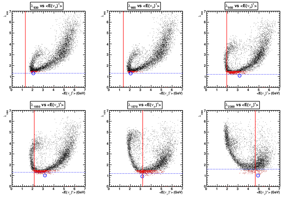
The results are not greatly changed by the general search though some gain appears to be visible for baselines larger than 1000 km. Blu markers highlight the configuration providing the best limit for each baseline. It turns out that the same configuration provides the best limit both for 630 and 665 km and the same happens for 950-1050 and 1570 km. We show the shapes of the horns for the three configurations in Fig. 7.

Given the limited improvement obtained with the general search, we decided to stick with the best candidates obtained with the fixed horn shape search. Choosing the configurations with the minimum has the disadvantage of being sensitive to down-going statistical fluctuations of 22 2 The statistical fluctuations become important especially for high energy fluxes due to single decays being assigned large weights. Anyway we checked that the result obtained with the general search gives similar results to the one which we obtain with the fixed horn search.
4 Neutrino fluxes from optimized focusing systems
The fluxes obtained with the optimized focusing setups according to the fixed shape search are shown in Fig. 833 3 Fluxes are publicly available on the internet [16]. For comparison they are all referred to a reference distance of 100 km. The mean energy increases roughly following the baseline increase. This is related, as already mentioned, to the fact that sitting at the maximum of oscillation allows to increase the statistics in the energy domain where the oscillation effects are more important. The energies of the oscillation maximum for each baseline (Fig. 1) are indicated with vertical lines having the same color as the corresponding spectrum. The corresponding integral muon neutrino fluxes values are given in the table at the right of Fig. 8. The flux increase as the mean energy increases can be intuitively explained considering that high energy pions are easier to focus since they naturally tend to emerge from the target in the forward direction and the neutrinos they produce have a higher chance to be in the far detector solid angle also thanks to the effect of the Lorentz boost. The regions of the pion phase space contributing to each flux are given in Fig. .

| optimiz. | flux |
|---|---|
| 130 | 0.38 |
| 630 | 1.59 |
| 665 | 1.81 |
| 950 | 2.69 |
| 1050 | 3.56 |
| 1570 | 3.93 |
| 2300 | 4.48 |
The muon neutrino charged current interaction rates corresponding to the presented fluxes are shown in Fig. 9 in the no-oscillation hypothesis (left) and accounting for the oscillation (right). They are normalized to a detector mass of 100 kton and a running time of one year corresponding to p.o.t. for the 50 GeV proton driver and p.o.t. for the 4.5 GeV option. The interaction rates without oscillation for the other neutrino flavors are given in Tab. 6.
The spectra are shown in the left plot of Fig. 9. Considerable samples of events could be collected with the fluxes optimized for the long baselines.
5 Physics performances with the optimized fluxes
| run | run | |||||||
|---|---|---|---|---|---|---|---|---|
| (Km) | ||||||||
| 130 | 41316 (94) | 174 (2) | / | 0.42 | 527 (5915) | 12 (15) | / | 0.42 |
| 630 | 36844 (2903) | 486 (95) | 28 | 1.5 | 7930 (13652) | 270 (157) | 11 | 2.0 |
| 665 | 38815 (2967) | 516 (96) | 28 | 1.5 | 7516 (14287) | 280 (158) | 11 | 2.0 |
| 950 | 37844 (1363) | 349 (48) | 40 | 1.0 | 3504 (14700) | 110 (107) | 15 | 1.3 |
| 1050 | 51787 (761) | 314 (23) | 148 | 0.64 | 1964 (21728) | 54 (88) | 65 | 0.60 |
| 1570 | 26785 (385) | 174 (10) | 170 | 0.67 | 945 (11184) | 22 (47) | 73 | 0.57 |
| 2300 | 17257 (203) | 110 (7) | 377 | 0.67 | 471 (7577) | 16 (32) | 172 | 0.60 |
| run | run | |||||||
|---|---|---|---|---|---|---|---|---|
| (Km) | ||||||||
| 130 | 41316 | 174 | / | 0.42 | 5915 | 15 | / | 0.42 |
| 630 | 36844 | 486 | 28 | 1.5 | 13652 | 157 | 11 | 2.0 |
| 665 | 38815 | 516 | 28 | 1.5 | 14287 | 158 | 11 | 2.0 |
| 950 | 37844 | 349 | 40 | 1.0 | 14700 | 107 | 15 | 1.3 |
| 1050 | 51787 | 314 | 148 | 0.64 | 21728 | 88 | 65 | 0.60 |
| 1570 | 26785 | 174 | 170 | 0.67 | 11184 | 47 | 73 | 0.57 |
| 2300 | 17257 | 110 | 377 | 0.67 | 7577 | 32 | 172 | 0.60 |
The expected sensitivities were computed with the help of the GLoBES [18] software. The detector response is described in GLoBES by assigning values for the energy resolution, efficiency and defining the considered channels.
The parametrization of the MEMPHYS detector which we used is the same which was used in [7] and is described in [19]. The event selection and particle identification are the Super-Kamiokande algorithms results. Migration matrices for the neutrino energy reconstruction are used to properly handle Fermi motion smearing and the non-QE event contamination. Reconstructed energy is divided into 100 MeV bins while the true neutrino energy in 40 MeV bins from 0 to 1.6 GeV. Four migration matrices for , , and are applied to signal events as well as backgrounds. Considered backgrounds are the interactions misidentified as , neutral current events and intrinsic components of the beam.
In the simulation of the GLACIER detector the considered backgrounds are the intrinsic and components in the beam. Reconstructed neutrino energy was divided in 100 MeV bins from 0 to 10 GeV. An constant energy resolution of 1 % is assumed for the signal and the background.
Running periods of 2 years in neutrino mode and 8 years in anti-neutrino mode were assumed. The parameters used in the calculation of the limits with GLoBES are summarized in Tab. 7
| MEMPHYS | GLACIER | |
|---|---|---|
| - running | 2-8 y | 2-8 y |
| Fit range | [0,1.6] GeV | [0,10] GeV |
| Bin width | 40 MeV | 100 MeV |
| Energy resolution | migr. matr. | 1% |
| Syst. err. | 2-5 % | 5% |
5.1 Sensitivity limits on
In order to discover a non-vanishing , the hypothesis = 0 must be excluded at the given C.L. As input, a true non-vanishing value of is chosen in the simulation and a fit with = 0 is performed, yielding the “discovery” potential. This procedure is repeated for every point in the ( , ) plane. The corresponding sensitivity to discover in the true ( , ) plane at 3 is shown in Fig. 10.
5.2 CP violation reach
By definition, the CP-violation in the lepton sector can be said to be discovered if the CP- conserving values, and , can be excluded at a given C.L. The reach for discovering CP-violation is computed choosing a “true” value for (= 0) as input at different true values of in the ( , ) plane, and for each point of the plane calculating the corresponding event rates expected in the experiment. This data is then fitted with the two CP-conserving values = 0 and = , leaving all other parameters free (including and ). The opposite mass hierarchy is also fitted and the minimum of all cases is taken as final . The corresponding sensitivity to discover CP-violation in the true ( , ) plane is shown in Fig. .
5.3 Determination of the mass hierarchy
In order to determine the mass hierarchy to a given C.L., the opposite mass hierarchy must be excluded. A point in parameter space with normal hierarchy is therefore chosen as true value and the solution with the smallest value with inverted hierarchy has to be determined by global minimization of the function leaving all oscillation parameters free within their priors. The sensitivity to exclude inverted mass hierarchy in the true ( , ) plane is shown in Fig. 12.
6 Conclusions
In this work we presented a comparison between the physics performance obtainable at the LAGUNA baselines in terms of discovery potential for , CP violation and mass hierarchy. We investigated two options for the proton driver: the high power SPL at 4.5 GeV and a high power PS2 at 50 GeV and two options for the detector technology: a 440 kton Water Cherenkov at 130 km (MEMPHYS) and a 100 kton LAr TPC (GLACIER) at longer baselines. The flux simulation profits of a full GEANT4 simulation which has been recently developed. Several cross checks of the algorithm have been presented. An systematic procedure of optimization of the focusing system for each baseline has been presented. With respect to previous studies in this case all the results come from an homogeneous set of tools.
Sensitivity limits obtainable with the high energy and the low energy super-beams are comparable if we assume for both a 5% systematic error on the fluxes. Concerning the high-energy super beam, better exclusion limits are obtained for intermediate baselines from 950 to 1570 Km but the difference is not marked. Mass hierarchy determination strongly favours long baselines as expected.
7 Acknowledgements
The LAGUNA design study is financed by FP7 Research Infrastructure "Design Studies", Grant Agreement No. 212343 FP7-INFRA-2007-1. The author also benefitted from useful discussions with …
References
- [1]
See
http://www.laguna-science.eu/. - [2] A. de Bellefon et al., MEMPHYS: A large scale water Cerenkov detector at Fréjus, arXiv:hep-ex/0607026.
- [3] A. Rubbia, Experiments for CP-violation: A giant liquid argon scintillation, Cherenkov and charge imaging experiment arXiv:hep-ph/0402110.
- [4] A. Rubbia, A CERN-based high-intensity high-energy proton source for long baseline neutrino oscillation experiments with next-generation large underground detectors for proton decay searches and neutrino physics and astrophysics, arXiv:hep-ph/1003.1921v1. 9 Mar 2010.
- [5] M. Mezzetto Physics potential of the SPL Super Beam J. Phys. G29 (2003),1781-1784, hep-ex/0302005.
- [6] J.E. Campagne, A. Cazes. The and sensitivities of the SPL-Fréjus project revisited Eur. Phys. J. C45 (2006)
- [7] J.E. Campagne, M. Maltoni, M. Mezzetto, T.Schwetz, Physics potential of the CERN-MEMPHYS neutrino oscillation project (2006), hep-ph/0603172.
- [8] GEANT 4 Nuclear Instruments and Methods in Physics Research A 506 (2003) 250-303 IEEE Transactions on Nuclear Science 53 No. 1 (2006) 270-278
- [9] A. Longhin, A new beamline design for a low-energy Super-Beam. In preparation.
- [10] M.Bonesini, A. Marchionni, F. Pietropaolo and T. Tabarelli de Fatis. On particle production for high energy neutrino beams hep-ph/0101163, Eur. Phys. J. C 20:13-27, 2001.
- [11] CERN PS2 working group. See https://paf-ps2.web.cern.ch/
- [12] L. Oberauer, F. von Feilitzsch and W. Potzel, A large liquid scintillator detector for low-energy neutrino astronomy, Nucl. Phys. Proc. Suppl. 138 (2005) 108.
- [13]
http://enrico1.physics.indiana.edu/messier/off-axis/spectra,messier@indiana.edu - [14]
T. Hasegawa, Plans for super-beams in Japan, arXiv:1001.0452 [hep-ex]. To appear in CERN Yellow Report - Future neutrino physics workshop, October 2009. Available at
http://jnusrv01.kek.jp/~hasegawa/pub/cernreport.pdf - [15] M. Baylac et al., Conceptual design of the SPL II: A high-power superconducting H- linac at CERN, CERN-2006-006.
- [16]
Fluxes in electronic format.
http://irfu.cea.fr/en/Phocea/Pisp/index.php?id=72 - [17] A. Longhin Study of the performance of the SPL-Fréjus Super Beam using a graphite target EURONU note EURONUnu-WP2-01. 15 May 2009.
- [18] Huber, M. Lindner and W. Winter, Simulation of long-baseline neutrino oscillation experiments with GLoBES, Comput. Phys. Commun. 167, 195 (2005)[arXiv:hep-ph/0407333].
- [19] GLOBES manual.