跳到论文正文
W Papers独立论文阅读器 arXiv:1206.4141 论文正文 计算阅读时间 · 0%
引用这篇论文根据当前论文元数据生成,正式投稿前建议核对。


License: arXiv.org perpetual non-exclusive license
arXiv:1206.4141v2 [hep-lat] 04 Oct 2012

Scattering phases for meson and baryon resonances on general moving-frame lattices

Preprint:  ADP-12-27/T794 DESY 12-098 Edinburgh 2012/09 LTH 948 June 2012
M. Göckeler1, R. Horsley2, M. Lage3, U.-G. Meißner3,4, P.E.L. Rakow5,
A. Rusetsky3, G. Schierholz6 and J.M. Zanotti7
Affiliation: 1 Institut für Theoretische Physik, Universität Regensburg, 93040 Regensburg, Germany

2 School of Physics and Astronomy, University of Edinburgh, Edinburgh EH9 3JZ, United Kingdom

3 Helmholtz-Institut für Strahlen- und Kernphysik (Theorie)
and Bethe Center for Theoretical Physics, Universität Bonn,
D-53115 Bonn, Germany

4 Institut für Kernphysik (IKP-3),
Institute for Advanced Simulation (IAS-4), Jülich Center for Hadron Physics and JARA – High Performance Computing,
Forschungszentrum Jülich, D-52425 Jülich, Germany

5 Theoretical Physics Division, Department of Mathematical Sciences, University of Liverpool, Liverpool L69 3BX, United Kingdom

6 Deutsches Elektronen-Synchrotron DESY, D-22603 Hamburg, Germany

7 CSSM, School of Chemistry and Physics, University of Adelaide, Adelaide SA 5005, Australia
Abstract

A proposal by Lüscher enables one to compute the scattering phases of elastic two-body systems from the energy levels of the lattice Hamiltonian in a finite volume. In this work we generalize the formalism to SS-, PP- and DD-wave meson and baryon resonances, and general total momenta. Employing nonvanishing momenta has several advantages, among them making a wider range of energy levels accessible on a single lattice volume and shifting the level crossing to smaller values of mπ​Lm_{\pi}L.

pacs
12.38.Gc

I Introduction

Most hadrons are resonances. Lattice simulations of QCD have reached the point now where the masses of up and down quarks are small enough so that the low-lying hadron resonances, such as the ρ⁡(770)\rho(770) and Δ⁡(1232)\Delta(1232), can decay via the strong interactions.

Extracting masses and widths of unstable particles from the lattice is made difficult by the fact that resonances cannot be identified directly with a single energy level of the lattice Hamiltonian. Rather, the eigenstates of the lattice Hamiltonian correspond to states that are characteristic of the respective volume. In a series of papers [1] Lüscher has derived the scattering phase shift in the infinite volume from the volume dependence of the energy levels of the lattice Hamiltonian.

Refer to caption
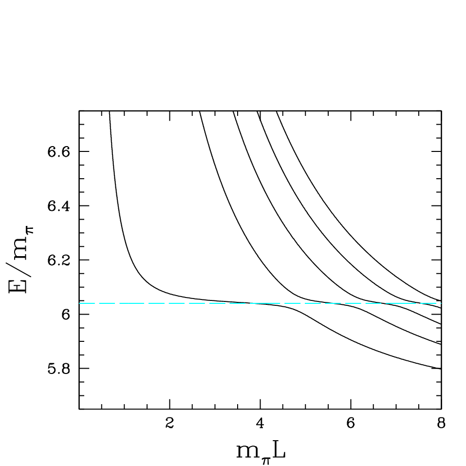
Figure 1: The ground state CM energy levels of the ρ\rho resonance at the physical point for various momenta 𝑷=(2​π/L)​𝒅\boldsymbol{P}=(2\pi/L)\,\boldsymbol{d}, together with the energy levels of the noninteracting π​π\pi\pi system. The horizontal dashed line indicates the physical mρ/mπm_{\rho}/m_{\pi} ratio.
Refer to captionRefer to caption
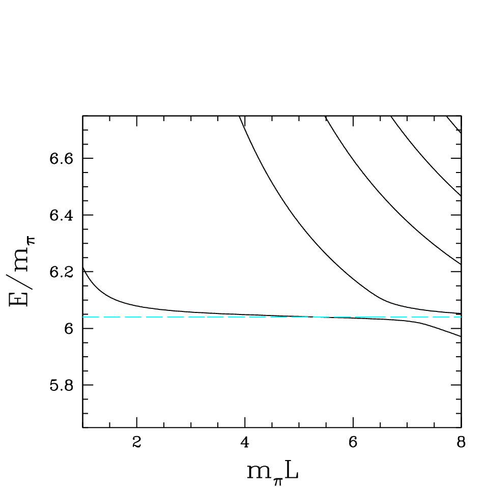
Figure 2: The expected five lowest CM energy levels of the Σ∗​(1385)\Sigma^{*}(1385) resonance at a pion mass of mπ=230​MeVm_{\pi}=230\,\mbox{MeV} [3] for zero total momentum (left) and 𝑷=2​π/L​𝒆3\boldsymbol{P}=2\pi/L\,\boldsymbol{e}_{3} (right). The dashed line indicates the anticipated mΣ∗/mπm_{\Sigma^{*}}/m_{\pi} ratio.

The original derivation was given for systems of two identical particles with vanishing total momentum. To compute the scattering phases for a sufficiently large set of energies on a rest-frame lattice, one would have to repeat the calculation on several volumes, which is computationally expensive.

If the total momentum of the resonance is nonzero, however, a wide variety of energy levels are becoming accessible on a single lattice volume, as has been realized by Gottlieb and Rummukainen [2]. This is illustrated in Fig. 1, where we show the expected ground state energy level of the ρ\rho resonance for several momenta at the physical pion mass, assuming an effective range approximation for the scattering phase with gρ​π​π=6.0g_{\rho\pi\pi}=6.0. At a lattice volume of mπ​L=2​…​2.5m_{\pi}L=2\ldots 2.5 the ground state energy levels of the four lowest momenta are found to cover the resonance region already sufficiently well. Figure 1 tells us, furthermore, that the energy levels of the interacting system rapidly approach the free particle energy spectrum as mπ​Lm_{\pi}L increases. For zero total momentum this limits the region of practical use to mπ​L≲2.5m_{\pi}L\lesssim 2.5, while for nonvanishing total momenta it extends to much larger values of mπ​Lm_{\pi}L.

Of particular interest to us are baryon resonances, which so far have not been explored at all. The low-lying baryon resonances have a much smaller phase space than, for example, the ρ\rho meson, which makes PP-wave resonances, such as the Δ\Delta and Σ∗\Sigma^{*}, especially hard to tackle. For zero total momentum and O⁡(200)​MeVO(200)\,\mbox{MeV} pion masses one would need volumes of L≈6​fmL\approx 6\,\mbox{fm} for the phase shift to cover the region δ≈π/2\delta\approx\pi/2. The reason is that the pion mass is so much smaller than the mass of the nucleon and the Λ\Lambda. Not so for nonzero total momenta though, which allows the pion to have zero momentum. In this case the avoided level crossing of the energy levels is shifted towards much smaller values of mπ​Lm_{\pi}L. This is illustrated in Fig. 2, where we compare the expected five lowest energy levels of the Σ∗\Sigma^{*} resonance, that decays to Λ​π\Lambda\pi, for zero and nonzero total momentum, assuming again an effective range approximation for the scattering phase with gΣ∗​Λ​π=9.2g_{\Sigma^{*}\Lambda\pi}=9.2.

Considering the difficulty of computing the properties of resonances on the lattice, how was ist possible that the mass spectrum of the pseudoscalar and vector meson octet and the baryon decuplet computed in [4, 3], using standard techniques, agreed so well with experiment? The answer is given in Fig. 2. In smaller, favorable volumes the ground state energy may agree well with the resonance mass over a wide range of mπ​Lm_{\pi}L. In larger volumes the ground state energy will approach the energy level of two free particles though.

Gottlieb and Rummukainen have extended Lüscher’s work on meson resonances to nonvanishing total momentum 𝑷=(2​π/L)​𝒆3\boldsymbol{P}=(2\pi/L)\,\boldsymbol{e}_{3}. Their work was generalized further to two-body systems of arbitrary mass by Davoudi and Savage [5] and Fu [6]. Recently, Feng et al. [7] have derived finite size formulae for the next higher momentum 𝑷=(2​π/L)​(𝒆1+𝒆2)\boldsymbol{P}=(2\pi/L)\,(\boldsymbol{e}_{1}+\boldsymbol{e}_{2}), which has been generalized again to particles of arbitrary masses by Leskovec and Prelovsek [8]. In the case of unequal masses and nonvanishing momenta the extraction of phase shifts from the energy levels of the lattice Hamiltonian proves difficult, because the partial waves of the individual scattering channels will mix in general. Strategies of how to overcome this problem have been discussed by Döring et al. [9] in the framework of unitarized chiral perturbation theory, which is equivalent to Lüscher’s approach in the large-LL limit. In this work we shall derive phase shift formulae for meson and baryon resonances for total momenta proportional to 𝑷=(2​π/L)​𝒆3\boldsymbol{P}=(2\pi/L)\,\boldsymbol{e}_{3}, 𝑷=(2​π/L)​(𝒆1+𝒆2)\boldsymbol{P}=(2\pi/L)\,(\boldsymbol{e}_{1}+\boldsymbol{e}_{2}) and 𝑷=(2​π/L)​(𝒆1+𝒆2+𝒆3)\boldsymbol{P}=(2\pi/L)\,(\boldsymbol{e}_{1}+\boldsymbol{e}_{2}+\boldsymbol{e}_{3}), including rotations of 𝑷\boldsymbol{P}. Our formulae will cover all two-body SS-, PP- and DD-wave meson and baryon resonances.

Knowing the scattering phase shifts for general total momenta, among others, we will be able to extract a great variety of other hadronic observables, including elastic and transition form factors of unstable particles, such as the ρ\rho form factor and the Δ\Delta to nucleon electromagnetic transition form factors.

The paper is organized as follows. Section II deals with the kinematics of two-particle states on the periodic lattice. In Sec. III we discuss the solutions of the Helmholtz equation for noninteracting and interacting particles. The Lorentz boost from the laboratory frame to the center of mass frame deforms the cubic lattice, and only some subgroups (little groups) of the original cubic point symmetry group remain. In Sec. IV we discuss the symmetry properties of the various center of mass frames, including the representations of the little groups. This is followed by the reduction of the phase shift formulae according to spin, angular momentum and representation in Sec. V. In Sec. VI we give explicit expressions for the phase shifts of the ρ\rho, Δ\Delta and N⋆​(1440)N^{\star}(1440) (Roper) resonances, and in Sec. VII we give a sample of operators that transform according to some of the prominent representations. Finally, in Sec. VIII we conclude.

II Two-particle kinematics on a moving-frame lattice

In this section we discuss the kinematical properties of two noninteracting particles of mass m1m_{1} and m2m_{2} in a cubic box of length LL with periodic boundary conditions. Twisted boundary conditions will be discussed elsewhere.

Let us first consider the lattice or laboratory (L) frame. We denote the 3-momenta of the individual particles by 𝒑1,𝒑2\boldsymbol{p}_{1},\boldsymbol{p}_{2}. The total momentum is denoted by 𝑷=𝒑1+𝒑2\boldsymbol{P}=\boldsymbol{p}_{1}+\boldsymbol{p}_{2}. The energy of two free particles is given by

W=𝒑12+m12+𝒑22+m22.W=\sqrt{\boldsymbol{p}_{1}^{2}+m_{1}^{2}}+\sqrt{\boldsymbol{p}_{2}^{2}+m_{2}^{2}}\,. (1)

The lattice momenta 𝒑i\boldsymbol{p}_{i} are quantized to

𝒑i=2​πL​𝒏i,𝒏i∈ℤ3,\boldsymbol{p}_{i}=\frac{2\pi}{L}\boldsymbol{n}_{i}\,,\quad\boldsymbol{n}_{i}\in\mathbb{Z}^{3}\,, (2)

and, similarly,

𝑷=2​πL​𝒅,𝒅∈ℤ3.\boldsymbol{P}=\frac{2\pi}{L}\boldsymbol{d}\,,\quad\boldsymbol{d}\in\mathbb{Z}^{3}\,. (3)

Next, we consider the center-of-mass (CM) frame, which is moving with velocity

𝒗=𝑷W,v=|𝒗|\boldsymbol{v}=\frac{\boldsymbol{P}}{W}\,,\quad v=|\boldsymbol{v}|\, (4)

in the laboratory frame. We denote the CM (relative) momentum by 𝒌\boldsymbol{k} and the energy by EE. Momentum and energy are obtained by a standard Lorentz transformation,

𝒌=𝜸⁡(𝒑1−𝒗​𝒑12+m12)=−𝜸⁡(𝒑2−𝒗​𝒑22+m22),\boldsymbol{k}=\boldsymbol{\gamma}\left(\boldsymbol{p}_{1}-\boldsymbol{v}\sqrt{\boldsymbol{p}_{1}^{2}+m_{1}^{2}}\right)=-\,\boldsymbol{\gamma}\left(\boldsymbol{p}_{2}-\boldsymbol{v}\sqrt{\boldsymbol{p}_{2}^{2}+m_{2}^{2}}\right)\,, (5)

where

𝜸​𝒑=γ​𝒑∥+𝒑⟂,γ=11−v2=WE\boldsymbol{\gamma}\boldsymbol{p}=\gamma\boldsymbol{p}_{\parallel}+\boldsymbol{p}_{\perp}\,,\quad\gamma=\frac{1}{\sqrt{1-v^{2}}}=\frac{W}{E} (6)

and

𝒑∥=𝒗​𝒗​𝒑v2,𝒑⟂=𝒑−𝒑∥.\boldsymbol{p}_{\parallel}=\boldsymbol{v}\;\frac{\boldsymbol{v}\boldsymbol{p}}{v^{2}}\,,\quad\boldsymbol{p}_{\perp}=\boldsymbol{p}-\boldsymbol{p}_{\parallel}\,. (7)

Laboratory and CM frame energies are related by

W=𝑷2+E2,W=\sqrt{\boldsymbol{P}^{2}+E^{2}}\,, (8)

where

E=E1+E2=𝒌2+m12+𝒌2+m22,𝒌2=(E2−(m12+m22))2−4​m12​m224​E2.E=E_{1}+E_{2}=\sqrt{\boldsymbol{k}^{2}+m_{1}^{2}}+\sqrt{\boldsymbol{k}^{2}+m_{2}^{2}}\,,\quad\boldsymbol{k}^{2}=\frac{\left(E^{2}-(m_{1}^{2}+m_{2}^{2})\right)^{2}-4m_{1}^{2}m_{2}^{2}}{4E^{2}}\,. (9)

Defining

𝒑=12​(𝒑1−𝒑2)=𝒑1−12​𝑷=−𝒑2+12​𝑷,\boldsymbol{p}=\frac{1}{2}\,\left(\boldsymbol{p}_{1}-\boldsymbol{p}_{2}\right)=\boldsymbol{p}_{1}-\frac{1}{2}\,\boldsymbol{P}=-\boldsymbol{p}_{2}+\frac{1}{2}\,\boldsymbol{P}\,, (10)

and expressing the laboratory frame energies in (5) by their CM counterparts, the CM momentum 𝒌\boldsymbol{k} can be rewritten as

𝒌=𝜸−1​𝒑−γ−1​m12−m22E2​12​𝑷,𝜸−1​𝒑=γ−1​𝒑∥+𝒑⟂.\boldsymbol{k}=\boldsymbol{\gamma}^{-1}\boldsymbol{p}-\gamma^{-1}\,\frac{m_{1}^{2}-m_{2}^{2}}{E^{2}}\,\frac{1}{2}\,\boldsymbol{P}\,,\quad\boldsymbol{\gamma}^{-1}\boldsymbol{p}=\gamma^{-1}\boldsymbol{p}_{\parallel}+\boldsymbol{p}_{\perp}\,. (11)

This results in the quantization condition

𝒌∈Γ𝚫\boldsymbol{k}\in\Gamma_{\boldsymbol{\Delta}} (12)

with

Γ𝚫={𝒌|𝒌=2​πL𝜸−1(𝒏−12𝚫),𝒏∈ℤ3},𝚫=𝒅(1+m12−m22E2).\Gamma_{\boldsymbol{\Delta}}=\left\{\boldsymbol{k}\,\Big|\,\boldsymbol{k}=\frac{2\pi}{L}\boldsymbol{\gamma}^{-1}\left(\boldsymbol{n}-\frac{1}{2}\,{\boldsymbol{\Delta}}\right)\,,\,\boldsymbol{n}\in\mathbb{Z}^{3}\right\}\,,\quad{\boldsymbol{\Delta}}=\boldsymbol{d}\,\left(1+\frac{m_{1}^{2}-m_{2}^{2}}{E^{2}}\right)\,. (13)

III Solutions of the Helmholtz equation

To compute the scattering phases of the interacting two-particle system, we need to discuss the solutions of the Helmholtz equation [10] in the CM frame first.

In the laboratory frame the two-particle state is described by the wave function ψL​(x1,x2)\psi_{L}(x_{1};x_{2}), where x1=(x10,𝒙1)x_{1}=(x^{0}_{1},\boldsymbol{x}_{1}), x2=(x20,𝒙2)x_{2}=(x^{0}_{2},\boldsymbol{x}_{2}) are the space-time coordinates in Minkowski space. For the moment we restrict ourselves to particles of spin zero. The wave function can then be written

ψL​(x1,x2)=e−i⁡(W​t−𝑷​𝑿)​ϕL​(x0,𝒙)\psi_{L}(x_{1};x_{2})=e^{-i(Wt-\boldsymbol{P}\boldsymbol{X})}\,\phi_{L}(x_{0},\boldsymbol{x}) (14)

with

𝑿=m1​𝒙1+m2​𝒙2m1+m2,𝒙=𝒙1−𝒙2,t=m1​x10+m2​x20m1+m2,x0=x10−x20.\begin{split}\boldsymbol{X}&=\frac{m_{1}\boldsymbol{x}_{1}+m_{2}\boldsymbol{x}_{2}}{m_{1}+m_{2}}\,,\quad\boldsymbol{x}=\boldsymbol{x}_{1}-\boldsymbol{x}_{2}\,,\\ t&=\frac{m_{1}x_{1}^{0}+m_{2}x_{2}^{0}}{m_{1}+m_{2}}\,,\quad x^{0}=x_{1}^{0}-x_{2}^{0}\,.\end{split} (15)

We are interested in the case where both particles have equal time coordinates, x10=x20=tx_{1}^{0}=x_{2}^{0}=t.

We denote the space-time separation in the CM frame by r=(r0,𝒓)r=(r^{0},\boldsymbol{r}). The transformation from the laboratory frame to the CM is given by

(r0𝒓)=(γ γ​𝒗𝜸𝒗 𝜸)​(0𝒙)\left(\begin{tabular}[]{c}$r^{0}$\\ $\boldsymbol{r}$\end{tabular}\right)=\left(\begin{tabular}[]{cc}$\gamma$&\,$\gamma\,\boldsymbol{v}$\\ $\boldsymbol{\gamma}\boldsymbol{v}$&\,$\boldsymbol{\gamma}$\end{tabular}\right)\,\left(\begin{tabular}[]{c}$0$\\ $\boldsymbol{x}$\end{tabular}\right) (16)

with

ϕL​(0,𝒙)=ϕC​M​(r0,𝒓).\phi_{L}(0,\boldsymbol{x})=\phi_{CM}(r^{0},\boldsymbol{r})\,. (17)

In the case of unequal masses, m1≠m2m_{1}\neq m_{2}, the (relative) time coordinate r0r^{0} is no longer zero, even though x0x^{0} is.

III.1 Noninteracting particles

For noninteracting particles the CM frame wave function obeys the equation of motion

(−∇r02+∇𝒓2+(E2−(m1+m2)2)​m1​m2(m1+m2)2)​ϕC​M​(r0,𝒓)=0\left(-\nabla^{2}_{r^{0}}+\boldsymbol{\nabla}^{2}_{\boldsymbol{r}}+\left(E^{2}-(m_{1}+m_{2})^{2}\right)\frac{m_{1}m_{2}}{(m_{1}+m_{2})^{2}}\right)\,\phi_{CM}(r^{0},\boldsymbol{r})=0 (18)

with

(−i​∇r0−E1​m2−E2​m1m1+m2)​ϕC​M​(r0,𝒓)=0.\left(-i\,\nabla_{r^{0}}-\frac{E_{1}m_{2}-E_{2}m_{1}}{m_{1}+m_{2}}\right)\,\phi_{CM}(r^{0},\boldsymbol{r})=0\,. (19)

Equations (18) and (19) follow directly from the Klein-Gordon equations of the individual particles. Writing

ϕC​M​(r0,𝒓)=ei​E1​m2−E2​m1m1+m2​r0​ϕC​M​(0,𝒓),\phi_{CM}(r^{0},\boldsymbol{r})=e^{i\,\frac{E_{1}m_{2}-E_{2}m_{1}}{m_{1}+m_{2}}\,r^{0}}\,\phi_{CM}(0,\boldsymbol{r})\,, (20)

the time dependence can be factored out, and we obtain the Helmholtz equation

(∇𝒓2+𝒌2)​ϕC​M​(𝒓)=0\left(\boldsymbol{\nabla}^{2}_{\boldsymbol{r}}+\boldsymbol{k}^{2}\right)\,\phi_{CM}(\boldsymbol{r})=0 (21)

with ϕC​M​(𝒓)=ϕC​M​(0,𝒓)\phi_{CM}(\boldsymbol{r})=\phi_{CM}(0,\boldsymbol{r}), and 𝒌\boldsymbol{k} given by (13).

The laboratory frame wave function is periodic under spatial translations

ψL​(x10,𝒙1,x20,𝒙2)=ψL​(x10,𝒙1+𝒏1​L,x20,𝒙2+𝒏2​L),𝒏1,2∈ℤ3.\psi_{L}(x_{1}^{0},\boldsymbol{x}_{1};x_{2}^{0},\boldsymbol{x}_{2})=\psi_{L}(x_{1}^{0},\boldsymbol{x}_{1}+\boldsymbol{n}_{1}L;x_{2}^{0},\boldsymbol{x}_{2}+\boldsymbol{n}_{2}L)\,,\quad\boldsymbol{n}_{1,2}\in\mathbb{Z}^{3}. (22)

Equations (14), (17) and (20) together give

ψL​(0,𝒙1,0,𝒙2)=ei⁡(𝑷​𝑿+E1​m2−E2​m1E⁡(m1+m2)​𝑷​𝒙)​ϕC​M​(𝒓),\psi_{L}(0,\boldsymbol{x}_{1};0,\boldsymbol{x}_{2})=e^{i\,\left(\boldsymbol{P}\boldsymbol{X}+\frac{E_{1}m_{2}-E_{2}m_{1}}{E(m_{1}+m_{2})}\boldsymbol{P}\boldsymbol{x}\right)}\,\phi_{CM}(\boldsymbol{r})\,, (23)

where we have inserted r0=γ​𝒗​𝒙=𝑷​𝒙/Er^{0}=\gamma\,\boldsymbol{v}\boldsymbol{x}=\boldsymbol{P}\boldsymbol{x}/E. This leads to the periodicity relation for the CM wave function

ϕC​M​(𝒓)=e−i​π​𝒏​𝚫​ϕC​M​(𝒓+𝜸​𝒏​L)\phi_{CM}(\boldsymbol{r})=e^{-i\,\pi\,\boldsymbol{n}{\boldsymbol{\Delta}}}\,\phi_{CM}(\boldsymbol{r}+\boldsymbol{\gamma}\boldsymbol{n}L) (24)

with 𝒏=𝒏1−𝒏2\boldsymbol{n}=\boldsymbol{n}_{1}-\boldsymbol{n}_{2}. While for equal masses ϕC​M​(𝒓)\phi_{CM}(\boldsymbol{r}) is either periodic (𝒏\boldsymbol{n} even) or antiperiodic (𝒏\boldsymbol{n} odd) with period γ​L\gamma L, this is no longer so for m1≠m2m_{1}\neq m_{2}. In this case the CM wave function picks up a complex phase factor e−i​π​𝒏​𝚫e^{-i\,\pi\,\boldsymbol{n}{\boldsymbol{\Delta}}} when crossing the spatial boundary. We call this attribute 𝚫{\boldsymbol{\Delta}}-periodic.

III.2 Interacting particles

Let us now turn to the interacting case. We assume that the two-body interaction has finite range and vanishes outside the region |𝒓|>R|\boldsymbol{r}|>R with L≫2​RL\gg 2R. In the exterior region ϕC​M​(𝒓)\phi_{CM}(\boldsymbol{r}) satisfies the Helmholtz equation

(∇𝒓2+𝒌2)​ϕC​M​(𝒓)=0\left(\boldsymbol{\nabla}^{2}_{\boldsymbol{r}}+\boldsymbol{k}^{2}\right)\,\phi_{CM}(\boldsymbol{r})=0 (25)

with

𝒌2=(E2−(m12+m22))2−4​m12​m224​E2≡k2,\boldsymbol{k}^{2}=\frac{\left(E^{2}-(m_{1}^{2}+m_{2}^{2})\right)^{2}-4m_{1}^{2}m_{2}^{2}}{4E^{2}}\equiv k^{2}\,, (26)

where EE now are the energy levels of the interacting system.

We are now looking for solutions of the Helmholtz equation (25). The (singular) case 𝒌∈Γ𝚫\boldsymbol{k}\in\Gamma_{\boldsymbol{\Delta}} requires a separate discussion, which we shall omit here. The Green function

G𝚫​(𝒓,k2)=γ−1​L−3​∑𝒑∈Γ𝚫ei​𝒑​𝒓𝒑2−k2G^{\boldsymbol{\Delta}}(\boldsymbol{r},k^{2})=\gamma^{-1}L^{-3}\sum_{\boldsymbol{p}\in\Gamma_{\boldsymbol{\Delta}}}\frac{e^{\,i\,\boldsymbol{p}\boldsymbol{r}}}{\boldsymbol{p}^{2}-k^{2}} (27)

is such a solution. An appropriate basis of solutions of the Helmholtz equation is obtained from (27) by

Gl​m𝚫​(𝒓,k2)=𝒴l​m​(∇)​G𝚫​(𝒓,k2),G^{\boldsymbol{\Delta}}_{lm}(\boldsymbol{r},k^{2})=\mathcal{Y}_{lm}(\boldsymbol{\nabla})\,G^{\boldsymbol{\Delta}}(\boldsymbol{r},k^{2})\,, (28)

where

𝒴l​m​(𝒓)=|𝒓|l​Yl​m​(𝒓^),𝒓^=𝒓|𝒓|.\mathcal{Y}_{lm}(\boldsymbol{r})=|\boldsymbol{r}|^{l}\,Y_{lm}(\hat{\boldsymbol{r}})\,,\quad\hat{\boldsymbol{r}}=\frac{\boldsymbol{r}}{|\boldsymbol{r}|}\,. (29)

Obviously, G𝚫​(𝒓,k2)G^{\boldsymbol{\Delta}}(\boldsymbol{r},k^{2}) and Gl​m𝚫​(𝒓,k2)G^{\boldsymbol{\Delta}}_{lm}(\boldsymbol{r},k^{2}) are 𝚫{\boldsymbol{\Delta}}-periodic. The CM wave function can then be expanded as

ϕC​M​(𝒓)=∑l,mcl​m​Gl​m𝚫​(𝒓,k2),\phi_{CM}(\boldsymbol{r})=\sum_{l,m}c_{lm}\,G^{\boldsymbol{\Delta}}_{lm}(\boldsymbol{r},k^{2})\,, (30)

which may be interpreted as a partial wave expansion. The functions Gl​m𝚫G^{\boldsymbol{\Delta}}_{lm} can be expanded in spherical harmonics Yl​m​(θ,φ)Y_{lm}(\theta,\varphi) and spherical Bessel functions [11] nl​(k​r)n_{l}(kr), jl​(k​r)j_{l}(kr)

Gl​m𝚫​(𝒓,k2)=(−1)l​kl+14​π​[nl​(k​r)​Yl​m​(θ,φ)+∑l′=0∞∑m′=−l′l′Ml​m,l′​m′𝚫​jl′​(k​r)​Yl′​m′​(θ,φ)]G^{\boldsymbol{\Delta}}_{lm}(\boldsymbol{r},k^{2})=\frac{(-1)^{l}\,k^{l+1}}{4\pi}\left[n_{l}(kr)\,Y_{lm}(\theta,\varphi)+\sum_{l^{\prime}=0}^{\infty}\sum_{m^{\prime}=-l^{\prime}}^{l^{\prime}}M_{lm,l^{\prime}m^{\prime}}^{\boldsymbol{\Delta}}\,j_{l^{\prime}}(kr)\,Y_{l^{\prime}m^{\prime}}(\theta,\varphi)\right] (31)

with

Ml​m,l′​m′𝚫=(−1)l​γ−1π3/2​∑j=|l−l′|l+l′∑s=−jjijqj+1​Zj​s𝚫​(1,q2)∗​Cl​m,j​s,l′​m′,q=k​L2​π,M_{lm,l^{\prime}m^{\prime}}^{\boldsymbol{\Delta}}=\frac{(-1)^{l}\,\gamma^{-1}}{\pi^{3/2}}\sum_{j=|l-l^{\prime}|}^{l+l^{\prime}}\,\sum_{s=-j}^{j}\frac{i^{j}}{q^{j+1}}\,Z_{js}^{\boldsymbol{\Delta}}(1,q^{2})^{*}\,C_{lm,js,l^{\prime}m^{\prime}}\,,\quad q=\frac{kL}{2\pi}\,, (32)

where r=|𝒓|,θr=|\boldsymbol{r}|,\theta and φ\varphi are the polar coordinates of 𝒓\boldsymbol{r}. The generalized zeta function Zj​s𝚫​(1,q2)Z_{js}^{\boldsymbol{\Delta}}(1,q^{2}) is obtained from

Zj​s𝚫​(δ,q2)=∑𝒛∈P𝚫𝒴j​s​(𝒛)(𝒛2−q2)δZ_{js}^{\boldsymbol{\Delta}}(\delta,q^{2})=\sum_{\boldsymbol{z}\in P_{\boldsymbol{\Delta}}}\frac{\mathcal{Y}_{js}(\boldsymbol{z})}{(\boldsymbol{z}^{2}-q^{2})^{\delta}} (33)

with

P𝚫={𝒛|𝒛=𝜸−1(𝒏−12𝚫),𝒏∈ℤ3}P_{\boldsymbol{\Delta}}=\left\{\boldsymbol{z}\,\Big|\,\boldsymbol{z}=\boldsymbol{\gamma}^{-1}\left(\boldsymbol{n}-\frac{1}{2}\,{\boldsymbol{\Delta}}\right)\,,\,\boldsymbol{n}\in\mathbb{Z}^{3}\right\} (34)

by analytic continuation δ→1\delta\rightarrow 1. The coefficient Cl​m,j​s,l′​m′C_{lm,js,l^{\prime}m^{\prime}} can be expressed in terms of Wigner 3​j3j-symbols

000).C_{lm,js,l^{\prime}m^{\prime}}=(-1)^{m^{\prime}}\,i^{l-j+l^{\prime}}\sqrt{(2l+1)(2j+1)(2l^{\prime}+1)}\left(\begin{tabular}[]{ccr}$l$&$j$&$l^{\prime}$\\ $m$&$s$&$-m^{\prime}$\end{tabular}\right)\,\left(\begin{tabular}[]{ccc}$l$&$j$&$l^{\prime}$\\ $0$&$0$&$0$\end{tabular}\right)\,.
Cl​m,j​s,l′​m′=(−1)m′​il−j+l′​(2​l+1)​(2​j+1)​(2​l′+1)​(ljl′ms−m′)​( ljl′ (35)

In Appendix A we give Zj​s𝚫​(1,q2)Z_{js}^{\boldsymbol{\Delta}}(1,q^{2}) for arbitrary values of jj and ss.

It is easily seen that

{𝒛|𝒛=𝜸−1(𝒏−12𝚫(m1,m2)),𝒏∈ℤ3}={−𝒛|𝒛=𝜸−1(𝒏−12𝚫(m2,m1)),𝒏∈ℤ3}.\begin{split}&\left\{\boldsymbol{z}\,\Big|\,\boldsymbol{z}=\boldsymbol{\gamma}^{-1}\left(\boldsymbol{n}-\frac{1}{2}\,{\boldsymbol{\Delta}}(m_{1},m_{2})\right)\,,\,\boldsymbol{n}\in\mathbb{Z}^{3}\right\}\\[5.0pt] &=\left\{-\boldsymbol{z}\,\Big|\,\boldsymbol{z}=\boldsymbol{\gamma}^{-1}\left(\boldsymbol{n}-\frac{1}{2}\,{\boldsymbol{\Delta}}(m_{2},m_{1})\right)\,,\,\boldsymbol{n}\in\mathbb{Z}^{3}\right\}\,.\end{split} (36)

This results in

Zj​s𝚫⁡(m1,m2)​(δ,q2)=(−1)j​Zj​s𝚫⁡(m2,m1)​(δ,q2)Z_{js}^{{\boldsymbol{\Delta}}(m_{1},m_{2})}(\delta,q^{2})=(-1)^{j}\,Z_{js}^{{\boldsymbol{\Delta}}(m_{2},m_{1})}(\delta,q^{2}) (37)

and

Ml​m,l′​m′𝚫⁡(m1,m2)=(−1)l+l′​Ml​m,l′​m′𝚫⁡(m2,m1),M_{lm,l^{\prime}m^{\prime}}^{{\boldsymbol{\Delta}}(m_{1},m_{2})}=(-1)^{l+l^{\prime}}\,M_{lm,l^{\prime}m^{\prime}}^{{\boldsymbol{\Delta}}(m_{2},m_{1})}\,, (38)

as l+j+l′=evenl+j+l^{\prime}=\mbox{even}. Both Ml​m,l′​m′𝚫⁡(m1,m2)M_{lm,l^{\prime}m^{\prime}}^{{\boldsymbol{\Delta}}(m_{1},m_{2})} and Ml​m,l′​m′𝚫⁡(m2,m1)M_{lm,l^{\prime}m^{\prime}}^{{\boldsymbol{\Delta}}(m_{2},m_{1})} have the same determinant and lead to the same results, so that the order of m1m_{1} and m2m_{2} does not matter.

In the literature one often finds the expression [2, 8]

Ml​m,l′​m′𝚫=(−1)l​γ−1π3/2​∑j=|l−l′|l+l′∑s=−jjijqj+1​Zj​s𝚫​(1,q2)​Cl​m,j​s,l′​m′.M_{lm,l^{\prime}m^{\prime}}^{\boldsymbol{\Delta}}=\frac{(-1)^{l}\,\gamma^{-1}}{\pi^{3/2}}\sum_{j=|l-l^{\prime}|}^{l+l^{\prime}}\,\sum_{s=-j}^{j}\frac{i^{j}}{q^{j+1}}\,Z_{js}^{\boldsymbol{\Delta}}(1,q^{2})\,C_{lm,js,l^{\prime}m^{\prime}}\,. (39)

Though not quite correct in general, it leads to the same results for the phase shifts as the matrix (32). Indeed, if we denote (39) by M~\tilde{M}, we find M~l​m,l′​m′=(−1)l+l′​Ml​m,l′​m′∗\tilde{M}_{lm,l^{\prime}m^{\prime}}=(-1)^{l+l^{\prime}}\,M_{lm,l^{\prime}m^{\prime}}^{*}, which has the same determinant as MM (see the equations for the phase shifts given in (54) and (55) below). In the following we shall use the short-hand notation

wl​m=1π3/2​2​l+1​γ−1​q−l−1​Zl​m𝚫​(1,q2).w_{lm}=\frac{1}{\pi^{3/2}\sqrt{2l+1}}\gamma^{-1}q^{-l-1}\,Z_{lm}^{\boldsymbol{\Delta}}(1,q^{2})\,. (40)

So far we have considered spinless particles only. Let us now assume that one of the particles carries spin SS. In the outer region |𝒓|>R|\boldsymbol{r}|>R, which we are concerned with here, the spin operator S^\hat{S} commutes with the Hamiltonian. The spin-dependent part of the wave function can thus be factored out. As we are mainly interested in meson-baryon resonances, we consider S=1/2S=1/2. In this case we have

ϕC​M(𝒓)=∑J,μl,m,σ⟨lm,12σ|Jμ⟩cl​mGl​m𝚫(𝒓,q2)χσ12,\phi_{CM}(\boldsymbol{r})=\sum_{\begin{subarray}{c}J,\mu\\ l,m,\sigma\end{subarray}}\langle lm,\frac{1}{2}\sigma|J\mu\rangle\,c_{lm}\,G_{lm}^{\boldsymbol{\Delta}}(\boldsymbol{r},q^{2})\,\chi_{\sigma}^{\frac{1}{2}}\,, (41)

where χσ12\chi^{\frac{1}{2}}_{\sigma} is the two-component baryon spinor. This amounts to an expansion of the CM wave function in terms of spin sperical harmonics

YJ​l​μ=∑m,σ⟨lm,12σ|Jμ⟩Yl​mχσ12.Y_{Jl\mu}=\sum_{m,\sigma}\langle lm,\frac{1}{2}\sigma|J\mu\rangle\,Y_{lm}\,\chi_{\sigma}^{\frac{1}{2}}\,. (42)

In this basis the matrix M𝚫M^{\boldsymbol{\Delta}} reads

MJ​l​μ,J′​l′​μ′𝚫=∑m,σm′,σ′⟨lm,12σ|Jμ⟩⟨l′m′,12σ′|J′μ′⟩Ml​m,l′​m′𝚫.M_{Jl\mu,J^{\prime}l^{\prime}\mu^{\prime}}^{\boldsymbol{\Delta}}=\sum_{\begin{subarray}{c}m,\sigma\\ m^{\prime},\sigma^{\prime}\end{subarray}}\langle lm,\frac{1}{2}\sigma|J\mu\rangle\,\langle l^{\prime}m^{\prime},\frac{1}{2}\sigma^{\prime}|J^{\prime}\mu^{\prime}\rangle\,M_{lm,l^{\prime}m^{\prime}}^{\boldsymbol{\Delta}}\,. (43)

IV Symmetry properties

The Lorentz boost deforms the cubic box to a parellelepiped, in which the length scale parallel to the direction of the boost vector is multiplied by γ\gamma, whereas the perpendicular length scale is left unchanged.

IV.1 Boost vectors

We will consider boost vectors

𝒅=(d1,d2,d3),di=0,±1\boldsymbol{d}=(d_{1},d_{2},d_{3})\,,\quad d_{i}=0,\pm 1 (44)

and integer multiples n​𝒅n\,\boldsymbol{d}, n∈ℤn\in\mathbb{Z} thereof. For that purpose it is sufficient to consider

𝒅=(0,0,0)≡ 0\boldsymbol{d}=(0,0,0)\,\equiv\,{\bf 0}  , 𝒅=(0,0,1)≡𝒆3\boldsymbol{d}=(0,0,1)\,\equiv\,\boldsymbol{e}_{3}  ,
𝒅=(1,1,0)≡𝒆1+𝒆2\boldsymbol{d}=(1,1,0)\,\equiv\,\boldsymbol{e}_{1}+\boldsymbol{e}_{2}  , 𝒅=(1,1,1)≡𝒆1+𝒆2+𝒆3\boldsymbol{d}=(1,1,1)\,\equiv\,\boldsymbol{e}_{1}+\boldsymbol{e}_{2}+\boldsymbol{e}_{3}  .
(45)

The boost vectors (44) can be transformed into one of the boost vectors (45) by a global rotation, which will leave our final results unchanged. Results for multiples of (45) are obtained by simply replacing 𝒅\boldsymbol{d} by n​𝒅n\,\boldsymbol{d} in the formulae to follow. In Fig. 3 we show two examples of the deformation of the cubic box.

Refer to captionRefer to caption
Figure 3: A cubic box of unit length deformed to a parallelepiped with 𝒅=(𝒆1+𝒆2)\boldsymbol{d}=(\boldsymbol{e}_{1}+\boldsymbol{e}_{2}) (left panel) and 𝒅=(𝒆1+𝒆2+𝒆3)\boldsymbol{d}=(\boldsymbol{e}_{1}+\boldsymbol{e}_{2}+\boldsymbol{e}_{3}) (right panel) for γ=2\gamma=2.

IV.2 Properties of the functions 𝒘𝒍​𝒎\mathbold{w_{lm}}

In the following we shall use the shorthand notation

𝒘l=(wl​l,wl​l−1,⋯wl−l+1,wl−l).\displaystyle\boldsymbol{w}_{l}=(w_{l\,l},w_{l\,l-1},\cdots w_{l\,-l+1},w_{l\,-l})\,. (46)

As a result of (37), wl​mw_{lm} is no longer zero for odd values of ll in the case of unequal masses. In general we have

Zl−m𝚫​(1,q2)=(−1)m​Zl​m𝚫​(1,q2)∗.\displaystyle Z^{{\boldsymbol{\Delta}}}_{l-m}(1;q^{2})=(-1)^{m}Z^{{\boldsymbol{\Delta}}}_{lm}(1;q^{2})^{*}\,. (47)

IV.2.1 The case 𝒅=(0,0,1)\boldsymbol{d}=(0,0,1)

In this case the system is symmetric under rotations around 𝒆3\boldsymbol{e}_{3} by π/2\pi/2, which leads to

Zl​m𝚫​(1,q2)=0,for​m≠0mod4.\displaystyle Z^{{\boldsymbol{\Delta}}}_{lm}(1;q^{2})=0\,,\quad\mbox{for}\;m\neq 0\mod 4\,. (48)

Furthermore, the system is symmetric under the interchange of axes 1↔21\leftrightarrow 2, as well as reflections 𝒆1,2→−𝒆1,2\boldsymbol{e}_{1,2}\rightarrow-\boldsymbol{e}_{1,2}. This leaves us with the following elements

ll 𝒘l\boldsymbol{w}_{l}
0 (w00)(w_{00})
1 (0,w10,0)(0,w_{10},0)
2 (0,0,w20,0,0)(0,0,w_{20},0,0)
3 (0,0,0,w30,0,0,0)(0,0,0,w_{30},0,0,0)
4 (w44,0,0,0,w40,0,0,0,w44)(w_{44},0,0,0,w_{40},0,0,0,w_{44})

IV.2.2 The case 𝒅=(1,1,0)\boldsymbol{d}=(1,1,0)

In this case the system is symmetric under the interchange of the axes 1↔21\leftrightarrow 2. Furthermore, the system is symmetric under reflections 𝒆3→−𝒆3\boldsymbol{e}_{3}\rightarrow-\boldsymbol{e}_{3}. This leaves us with the following elements

ll 𝒘l\boldsymbol{w}_{l}
0 (w00)(w_{00})
1 2Rew11(ei​π/4,0,−e−iπ/4)\sqrt{2}\,{\rm Re}\,w_{11}\,\left(e^{i\pi/4},0,-e^{-i\pi/4}\right)
2 (w22,0,w20,0,−w22)(w_{22},0,w_{20},0,-w_{22})
3 2(e−iπ/4Rew33,0,ei​π/4Rew31,0,−e−iπ/4Rew31,0,−ei​π/4Rew33)\sqrt{2}\,\left(e^{-i\pi/4}{\rm Re}\,w_{33},0,e^{i\pi/4}{\rm Re}\,w_{31},0,-e^{-i\pi/4}{\rm Re}\,w_{31},0,-e^{i\pi/4}{\rm Re}\,w_{33}\right)
4 (w44,0,w42,0,w40,0,−w42,0,w44)(w_{44},0,w_{42},0,w_{40},0,-w_{42},0,w_{44})

IV.2.3 The case 𝒅=(1,1,1)\boldsymbol{d}=(1,1,1)

In this case the only symmetry that is left is the symmetry under cyclic permutation 1→2→3→11\rightarrow 2\rightarrow 3\rightarrow 1. This leaves us with the following elements

ll 𝒘l\boldsymbol{w}_{l}
0 (w00)(w_{00})
1 w10(−ei​π/4,1,e−iπ/4)w_{10}\,\left(-e^{i\pi/4},1,e^{-i\pi/4}\right)
2 w22(1,−2e−iπ/4,0,−2ei​π/4,−1)w_{22}\,\left(1,-\sqrt{2}e^{-i\pi/4},0,-\sqrt{2}e^{i\pi/4},-1\right)
3 (−104e−iπ/4w30,w32,64ei​π/4w30,w30,−64e−iπ/4w30,−w32,104ei​π/4w30)\left(-\frac{\sqrt{10}}{4}\,e^{-i\pi/4}w_{30},w_{32},\frac{\sqrt{6}}{4}\,e^{i\pi/4}\,w_{30},w_{30},-\frac{\sqrt{6}}{4}\,e^{-i\pi/4}\,w_{30},-w_{32},\frac{\sqrt{10}}{4}\,e^{i\pi/4}w_{30}\right)
4 (7014w40,−72ei​π/4w42,w42,12e−iπ/4w42,w40,12ei​π/4w42,−w42,−72e−iπ/4w42,7014w40)\left(\frac{\sqrt{70}}{14}\,w_{40},-\frac{\sqrt{7}}{2}\,e^{i\pi/4}w_{42},w_{42},\frac{1}{2}\,e^{-i\pi/4}w_{42},w_{40},\frac{1}{2}\,e^{i\pi/4}w_{42},-w_{42},-\frac{\sqrt{7}}{2}\,e^{-i\pi/4}w_{42},\frac{\sqrt{70}}{14}\,w_{40}\right)

IV.3 Irreducible representations of the little groups

In the CM frame, the symmetry group of the cubic lattice is the cubic group OO for particles with integer spin, and its double cover group O2{}^{2}O for particles with half-integer spin. The group OO consists of 24 elements RiR_{i}, i.e. rotation matrices, which are characterized by the axis 𝒏(i)\boldsymbol{n}^{(i)} and angle ωi\omega_{i} of rotation (with i=1,⋯,24i=1,\cdots,24). The rotation matrices are given by

(Ri)α​β=cos⁡ωi​δα​β+(1−cos⁡ωi)​nα(i)​nβ(i)−sin⁡ωi​ϵα​β​γ​nγ(i),α,β,γ=1,2,3.\displaystyle(R_{i})_{\alpha\beta}=\cos\omega_{i}\,\delta_{\alpha\beta}+(1-\cos\omega_{i})\,n^{(i)}_{\alpha}n^{(i)}_{\beta}-\sin\omega_{i}\,\epsilon_{\alpha\beta\gamma}\,n^{(i)}_{\gamma}\,,\quad\alpha,\beta,\gamma=1,2,3\,. (49)

The 24 elements of OO fall into five different conjugacy classes. They are listed in Table 1. The group O2{}^{2}O has 48 elements RiR_{i}. As for OO, they are characterized by the axis 𝒏(i)\boldsymbol{n}^{(i)} and angle ωi\omega_{i} (with i=1,⋯,48i=1,\cdots,48 now). The 48 elements of O2{}^{2}O fall into eight different conjugacy classes. They are listed in Table 2.

Class ii 𝒏(i)\boldsymbol{n}^{(i)} ωi\omega_{i}
II 1 any 00
8​C38C_{3} 2 (1,1,1)/3(1,1,1)/\sqrt{3} −2π/3-2\pi/3
3 (1,1,1)/3(1,1,1)/\sqrt{3} 2​π/32\pi/3
4 (−1,1,1)/3(-1,1,1)/\sqrt{3} −2π/3-2\pi/3
5 (−1,1,1)/3(-1,1,1)/\sqrt{3} 2​π/32\pi/3
6 (−1,−1,1)/3(-1,-1,1)/\sqrt{3} −2π/3-2\pi/3
7 (−1,−1,1)/3(-1,-1,1)/\sqrt{3} 2​π/32\pi/3
8 (1,−1,1)/3(1,-1,1)/\sqrt{3} −2π/3-2\pi/3
9 (1,−1,1)/3(1,-1,1)/\sqrt{3} 2​π/32\pi/3
6​C46C_{4} 10 (1,0,0)(1,0,0) −π/2-\pi/2
11 (1,0,0)(1,0,0) π/2\pi/2
12 (0,1,0)(0,1,0) −π/2-\pi/2
13 (0,1,0)(0,1,0) π/2\pi/2
14 (0,0,1)(0,0,1) −π/2-\pi/2
15 (0,0,1)(0,0,1) π/2\pi/2
6​C2′6C^{\prime}_{2} 16 (0,1,1)/2(0,1,1)/\sqrt{2} −π-\pi
17 (0,−1,1)/2(0,-1,1)/\sqrt{2} −π-\pi
18 (1,1,0)/2(1,1,0)/\sqrt{2} −π-\pi
19 (1,−1,0)/2(1,-1,0)/\sqrt{2} −π-\pi
20 (1,0,1)/2(1,0,1)/\sqrt{2} −π-\pi
21 (−1,0,1)/2(-1,0,1)/\sqrt{2} −π-\pi
3​C23C_{2} 22 (1,0,0)(1,0,0) −π-\pi
23 (0,1,0)(0,1,0) −π-\pi
24 (0,0,1)(0,0,1) −π-\pi
Table 1: The elements of the cubic group, parameterized by the rotation axis 𝒏(i)\boldsymbol{n}^{(i)} and rotation angle ωi\omega_{i}, divided into the different conjugacy classes.
Class ii 𝒏(i)\boldsymbol{n}^{(i)} ωi\omega_{i} Class ii 𝒏(i)\boldsymbol{n}^{(i)} ωi\omega_{i}
II 1 any 00 8​C38C_{3} 28 (1,1,1)/3(1,1,1)/\sqrt{3} 4​π/34\pi/3
6​C46C_{4} 2 (1,0,0)(1,0,0) π\pi 29 (−1,1,1)/3(-1,1,1)/\sqrt{3} 4​π/34\pi/3
3 (0,1,0)(0,1,0) π\pi 30 (−1,−1,1)/3(-1,-1,1)/\sqrt{3} 4​π/34\pi/3
4 (0,0,1)(0,0,1) π\pi 31 (1,−1,1)/3(1,-1,1)/\sqrt{3} 4​π/34\pi/3
5 (1,0,0)(1,0,0) −π-\pi 32 (1,1,1)/3(1,1,1)/\sqrt{3} −4π/3-4\pi/3
6 (0,1,0)(0,1,0) −π-\pi 33 (−1,1,1)/3(-1,1,1)/\sqrt{3} −4π/3-4\pi/3
7 (0,0,1)(0,0,1) −π-\pi 34 (−1,−1,1)/3(-1,-1,1)/\sqrt{3} −4π/3-4\pi/3
6​C8′6C^{\prime}_{8} 8 (1,0,0)(1,0,0) π/2\pi/2 35 (1,−1,1)/3(1,-1,1)/\sqrt{3} −4π/3-4\pi/3
9 (0,1,0)(0,1,0) π/2\pi/2 12​C4′12C^{\prime}_{4} 36 (0,1,1)/2(0,1,1)/\sqrt{2} π\pi
10 (0,0,1)(0,0,1) π/2\pi/2 37 (0,−1,1)/2(0,-1,1)/\sqrt{2} π\pi
11 (1,0,0)(1,0,0) −π/2-\pi/2 38 (1,1,0)/2(1,1,0)/\sqrt{2} π\pi
12 (0,1,0)(0,1,0) −π/2-\pi/2 39 (1,−1,0)/2(1,-1,0)/\sqrt{2} π\pi
13 (0,0,1)(0,0,1) −π/2-\pi/2 40 (1,0,1)/2(1,0,1)/\sqrt{2} π\pi
6​C86C_{8} 14 (1,0,0)(1,0,0) 3​π/23\pi/2 41 (−1,0,1)/2(-1,0,1)/\sqrt{2} π\pi
15 (0,1,0)(0,1,0) 3​π/23\pi/2 42 (0,1,1)/2(0,1,1)/\sqrt{2} −π-\pi
16 (0,0,1)(0,0,1) 3​π/23\pi/2 43 (0,−1,1)/2(0,-1,1)/\sqrt{2} −π-\pi
17 (1,0,0)(1,0,0) −3π/2-3\pi/2 44 (1,1,0)/2(1,1,0)/\sqrt{2} −π-\pi
18 (0,1,0)(0,1,0) −3π/2-3\pi/2 45 (1,−1,0)/2(1,-1,0)/\sqrt{2} −π-\pi
19 (0,0,1)(0,0,1) −3π/2-3\pi/2 46 (1,0,1)/2(1,0,1)/\sqrt{2} −π-\pi
8​C68C_{6} 20 (1,1,1)/3(1,1,1)/\sqrt{3} 2​π/32\pi/3 47 (−1,0,1)/2(-1,0,1)/\sqrt{2} −π-\pi
21 (−1,1,1)/3(-1,1,1)/\sqrt{3} 2​π/32\pi/3 JJ 48 any 2​π2\pi
22 (−1,−1,1)/3(-1,-1,1)/\sqrt{3} 2​π/32\pi/3
23 (1,−1,1)/3(1,-1,1)/\sqrt{3} 2​π/32\pi/3
24 (1,1,1)/3(1,1,1)/\sqrt{3} −2π/3-2\pi/3
25 (−1,1,1)/3(-1,1,1)/\sqrt{3} −2π/3-2\pi/3
26 (−1,−1,1)/3(-1,-1,1)/\sqrt{3} −2π/3-2\pi/3
27 (1,−1,1)/3(1,-1,1)/\sqrt{3} −2π/3-2\pi/3
Table 2: The elements of the double cover group of the cubic group, parameterized by the rotation axis 𝒏(i)\boldsymbol{n}^{(i)} and rotation angle ωi\omega_{i}, divided into the different conjugacy classes.

The full symmetry group includes space inversions II, which commute with the elements of OO and O2{}^{2}O. Choosing T⁡(I)=−1T(I)=-1,11 1 Alternatively, we could have chosen T⁡(I)=1T(I)=1. Both choices are consistent with I2=1I^{2}=1. where T⁡(I)T(I) denotes an element of any matrix representation of II, the elements of OO and O2{}^{2}O combined with II form the product groups Oh=O⊗{1,−1}O_{h}=O\otimes\{1,-1\} and Oh2=O2⊗{1,−1}{}^{2}O_{h}={}^{2}O\otimes\{1,-1\}, respectively. Irreducible matrix representations of OhO_{h} and Oh2{}^{2}O_{h} have been given, for example, in [12].

In the CM frame moving with velocity 𝒗=𝑷/W\boldsymbol{v}=\boldsymbol{P}/W, 𝑷=(2​π/L)​𝒅\boldsymbol{P}=(2\pi/L)\,\boldsymbol{d} in the laboratory frame, the symmetry group reduces to certain subgroups of OhO_{h} and Oh2{}^{2}O_{h}, hereafter referred to as the little groups. In the case of unequal masses, the little group consists of elements Si={Ri,I​Ri}∈OhS_{i}=\{R_{i},IR_{i}\}\in O_{h} and Oh2{}^{2}O_{h}, respectively, which obey

Si​𝒅=𝒅.\displaystyle S_{i}\,\boldsymbol{d}=\boldsymbol{d}\,. (50)

In the case of equal masses, the system is symmetric under 𝒅→−𝒅\boldsymbol{d}\rightarrow-\boldsymbol{d}, and the little group consists of elements SiS_{i}, which obey

Si​𝒅=±𝒅.\displaystyle S_{i}\,\boldsymbol{d}=\pm\boldsymbol{d}\,. (51)

In Table 3 we list the elements Ri∈OR_{i}\in O and O2{}^{2}O that satisfy the condition Ri​𝒅=𝒅R_{i}\,\boldsymbol{d}=\boldsymbol{d} and Ri​𝒅=−𝒅R_{i}\,\boldsymbol{d}=-\boldsymbol{d} for our three choices of 𝒅\boldsymbol{d}, together with the corresponding little groups. With I​𝒅=−𝒅I\boldsymbol{d}=-\boldsymbol{d}, the action of the group elements SiS_{i} on 𝒅\boldsymbol{d} is now fully defined.

Group 𝒅\boldsymbol{d} Little Group Ri​𝒅=𝒅R_{i}\,\boldsymbol{d}=\boldsymbol{d} Ri​𝒅=−𝒅R_{i}\,\boldsymbol{d}=-\boldsymbol{d}
OhO_{h} (0,0,1)(0,0,1) C4​vC_{4v} {Ri|i=1,14,15,24}\{R_{i}|i=1,14,15,24\} {Ri|i=18,19,22,23}\{R_{i}|i=18,19,22,23\}
(1,1,0)(1,1,0) C2​vC_{2v} {Ri|i=1,18}\{R_{i}|i=1,18\} {Ri|i=19,24}\{R_{i}|i=19,24\}
(1,1,1)(1,1,1) C3​vC_{3v} {Ri|i=1,2,3}\{R_{i}|i=1,2,3\} {Ri|i=17,19,21}\{R_{i}|i=17,19,21\}
Oh2{}^{2}O_{h} (0,0,1)(0,0,1) C4​v2{}^{2}C_{4v} {Ri|i=1,4,7,10,13,16,19,48}\{R_{i}|i=1,4,7,10,13,16,19,48\} {Ri|i=2,3,5,6,38,39,44,45}\{R_{i}|i=2,3,5,6,38,39,44,45\}
(1,1,0)(1,1,0) C2​v2{}^{2}C_{2v} {Ri|i=1,38,44,48}\{R_{i}|i=1,38,44,48\} {Ri|i=4,7,39,45}\{R_{i}|i=4,7,39,45\}
(1,1,1)(1,1,1) C3​v2{}^{2}C_{3v} {Ri|i=1,20,24,28,32,48}\{R_{i}|i=1,20,24,28,32,48\} {Ri|i=37,39,41,43,45,47}\{R_{i}|i=37,39,41,43,45,47\}
Table 3: Rotations RiR_{i} that obey the condition Ri​𝒅=±𝒅R_{i}\,\boldsymbol{d}=\pm\boldsymbol{d}.

As we shall see, several of the irreducible representations of the little groups C4​vC_{4v}, C4​v2{}^{2}C_{4v}, C2​v2{}^{2}C_{2v}, C3​vC_{3v} and C3​v2{}^{2}C_{3v} in Table 3, namely EE, G1G_{1} and G2G_{2}, are two-dimensional. Two-dimensional representations G1G_{1} and G2G_{2} can be built from the matrices

(Yi)α​β=(e−i2​𝒏(i)​σ​ω𝒊)α​β=δα​β​cos⁡ωi2−i​(𝒏(i)​σ)α​β​sin⁡ωi2,α,β=1,2\displaystyle(Y_{i})_{\alpha\beta}=\left(e^{-\frac{i}{2}\,\boldsymbol{n}^{(i)}\mathbold{\sigma}\,\omega_{i}}\right)_{\alpha\beta}=\delta_{\alpha\beta}\,\cos\frac{\omega_{i}}{2}-i\,\left(\boldsymbol{n}^{(i)}\mathbold{\sigma}\right)_{\alpha\beta}\,\sin\frac{\omega_{i}}{2}\,,\quad\alpha,\beta=1,2 (52)

with i=1,⋯,48i=1,\cdots,48.

For the two-dimensional representation EE in the bosonic case, it is convenient to introduce the matrices

X1=𝟙,X2=−12 1+i32σ2,X3=−12 1−i32σ2,X4=−12σ3−32σ1,X5=σ3,X6=−12σ3+32σ1,X7=i12(σ1+σ2),X8=12(σ1−σ2).\begin{split}&X_{1}=\mathbbm{1}\,,\quad X_{2}=-\frac{1}{2}\,\mathbbm{1}+i\frac{\sqrt{3}}{2}\,\sigma_{2}\,,\quad X_{3}=-\frac{1}{2}\,\mathbbm{1}-i\frac{\sqrt{3}}{2}\,\sigma_{2}\,,\quad X_{4}=-\frac{1}{2}\,\sigma_{3}-\frac{\sqrt{3}}{2}\,\sigma_{1}\,,\quad\\ &X_{5}=\sigma_{3}\,,\quad X_{6}=-\frac{1}{2}\,\sigma_{3}+\frac{\sqrt{3}}{2}\,\sigma_{1}\,,\quad X_{7}=i\frac{1}{\sqrt{2}}\,(\sigma_{1}+\sigma_{2})\,,\quad X_{8}=\frac{1}{\sqrt{2}}\,(\sigma_{1}-\sigma_{2})\,.\end{split} (53)
{Si}\{S_{i}\} R1R_{1} {R14,R15}\{R_{14},R_{15}\} {I​R18,I​R19}\{IR_{18},IR_{19}\} {I​R22,I​R23}\{IR_{22},IR_{23}\} R24R_{24}
Γ II 2​C42C_{4} 2​I​C2′2IC_{2}^{\prime} 2​I​C22IC_{2} C2C_{2}
A1A_{1} 1 1 1 1 1
A2A_{2} 1 1 -1 -1 1
B1B_{1} 1 -1 -1 1 1
B2B_{2} 1 -1 1 -1 1
EE 2 0 0 0 -2
EE X1X_{1} {−X7,X7}\{-X_{7},X_{7}\} {X5,−X5}\{X_{5},-X_{5}\} {X8,−X8}\{X_{8},-X_{8}\} −X1-X_{1}
Table 4: Character table of the little group C4​vC_{4v} for integer spin. The top row shows the elements of C4​vC_{4v} divided into conjugacy classes. The bottom row shows the corresponding matrices for the two-dimensional irreducible representation EE. The rows in between list the characters of the various irreducible representations Γ\Gamma of C4​vC_{4v}.
{Si}\{S_{i}\} R1R_{1} {R4,R7}\{R_{4},R_{7}\} {R10,R13}\{R_{10},R_{13}\} {R16,R19}\{R_{16},R_{19}\} {I​R2,I​R3,I​R5,I​R6}\{IR_{2},IR_{3},IR_{5},IR_{6}\} {I​R38,I​R39,I​R44,I​R45}\{IR_{38},IR_{39},IR_{44},IR_{45}\} R48R_{48}
Γ II 2​C42C_{4} 2​C8′2C_{8}^{\prime} 2​C82C_{8} 4​I​C44IC_{4} 4​I​C4′4IC_{4}^{\prime} JJ
A1A_{1} 1 1 1 1 1 1 1
A2A_{2} 1 1 1 1 -1 -1 1
B1B_{1} 1 1 -1 -1 1 -1 1
B2B_{2} 1 1 -1 -1 -1 1 1
EE 2 -2 0 0 0 0 2
G1G_{1} 2 0 2\sqrt{2} −2-\sqrt{2} 0 0 -2
G2G_{2} 2 0 −2-\sqrt{2} 2\sqrt{2} 0 0 -2
EE 𝟙\mathbbm{1} {−𝟙,−𝟙}\{-\mathbbm{1},-\mathbbm{1}\} {i​σ3,−i​σ3}\{i\sigma_{3},-i\sigma_{3}\} {−i​σ3,i​σ3}\{-i\sigma_{3},i\sigma_{3}\} {σ1,−σ1,σ1,−σ1}\{\sigma_{1},-\sigma_{1},\sigma_{1},-\sigma_{1}\} {−σ2,σ2,−σ2,σ2}\{-\sigma_{2},\sigma_{2},-\sigma_{2},\sigma_{2}\} 𝟙\mathbbm{1}
G1G_{1} Y1Y_{1} {Y4,Y7}\{Y_{4},Y_{7}\} {Y10,Y13}\{Y_{10},Y_{13}\} {Y16,Y19}\{Y_{16},Y_{19}\} {−Y2,−Y3,−Y5,−Y6}\{-Y_{2},-Y_{3},-Y_{5},-Y_{6}\} {−Y38,−Y39,−Y44,−Y45}\{-Y_{38},-Y_{39},-Y_{44},-Y_{45}\} Y48Y_{48}
G2G_{2} Y1Y_{1} {Y4,Y7}\{Y_{4},Y_{7}\} {−Y10,−Y13}\{-Y_{10},-Y_{13}\} {−Y16,−Y19}\{-Y_{16},-Y_{19}\} {Y2,Y3,Y5,Y6}\{Y_{2},Y_{3},Y_{5},Y_{6}\} {−Y38,−Y39,−Y44,−Y45}\{-Y_{38},-Y_{39},-Y_{44},-Y_{45}\} Y48Y_{48}
Table 5: The same as Table 5 for the little group C4​v2{}^{2}C_{4v} and half-integer spin, together with the matrices of the two-dimensional irreducible representations EE, G1G_{1} and G2G_{2}.
SiS_{i} R1R_{1} R18R_{18} I​R19IR_{19} I​R24IR_{24}
Γ II C2′C_{2}^{\prime} I​C2′IC_{2}^{\prime} I​C2IC_{2}
A1A_{1} 1 1 1 1
A2A_{2} 1 1 -1 -1
B1B_{1} 1 -1 1 -1
B2B_{2} 1 -1 -1 1
Table 6: The same as Table 5 for the little group C2​vC_{2v} and integer spin.
{Si}\{S_{i}\} R1R_{1} {R38,R44}\{R_{38},R_{44}\} {I​R4,I​R7}\{IR_{4},IR_{7}\} {I​R39,I​R45}\{IR_{39},IR_{45}\} R48R_{48}
Γ II 2​C4′2C_{4}^{\prime} 4​I​C44IC_{4} 4​I​C4′4IC_{4}^{\prime} JJ
A1A_{1} 1 1 1 1 1
A2A_{2} 1 1 -1 -1 1
B1B_{1} 1 -1 -1 1 1
B2B_{2} 1 -1 1 -1 1
G1G_{1} 2 0 0 0 -2
G1G_{1} Y1Y_{1} {Y38,Y44}\{Y_{38},Y_{44}\} {−Y4,−Y7}\{-Y_{4},-Y_{7}\} {−Y39,−Y45}\{-Y_{39},-Y_{45}\} Y48Y_{48}
Table 7: The same as Table 5 for the little group C2​v2{}^{2}C_{2v} and half-integer spin, together with the matrices of the two-dimensional irreducible representation G1G_{1}.
{Si}\{S_{i}\} R1R_{1} {R2,R3}\{R_{2},R_{3}\} {I​R17,I​R19,I​R21}\{IR_{17},IR_{19},IR_{21}\}
Γ II 2​C32C_{3} 3​I​C2′3IC_{2}^{\prime}
A1A_{1} 1 1 1
A2A_{2} 1 1 -1
EE 2 -1 0
EE X1X_{1} {X2,X3}\{X_{2},X_{3}\} {−X4,−X5,−X6}\{-X_{4},-X_{5},-X_{6}\}
Table 8: The same as Table 5 for the little group C3​vC_{3v} and integer spin, together with the matrices of the two-dimensional irreducible representation EE.
{Si}\{S_{i}\} R1R_{1} {R20,R24}\{R_{20},R_{24}\} {R28,R32}\{R_{28},R_{32}\} {I​R37,I​R45,I​R47}\{IR_{37},IR_{45},IR_{47}\} {I​R39,I​R41,I​R43}\{IR_{39},IR_{41},IR_{43}\} R48R_{48}
Γ II 2​C62C_{6} 2​C32C_{3} 3​I​C43IC_{4} 3​I​C4′3IC_{4}^{\prime} JJ
A1A_{1} 1 1 1 1 1 1
A2A_{2} 1 1 1 -1 -1 1
K1K_{1} 1 -1 1 ii −i-i -1
K2K_{2} 1 -1 1 −i-i ii -1
EE 2 -1 -1 0 0 2
G1G_{1} 2 1 -1 0 0 -2
EE X1X_{1} {X3,X2}\{X_{3},X_{2}\} {X2,X3}\{X_{2},X_{3}\} {−X4,−X5,−X6}\{-X_{4},-X_{5},-X_{6}\} {−X5,−X6,−X4}\{-X_{5},-X_{6},-X_{4}\} X1X_{1}
G1G_{1} Y1Y_{1} {Y20,Y24}\{Y_{20},Y_{24}\} {Y28,Y32}\{Y_{28},Y_{32}\} {−Y37,−Y45,−Y47}\{-Y_{37},-Y_{45},-Y_{47}\} {−Y39,−Y41,−Y43}\{-Y_{39},-Y_{41},-Y_{43}\} Y48Y_{48}
Table 9: The same as Table 5 for the little group C3​v2{}^{2}C_{3v} and half-integer spin, together with the matrices of the two-dimensional irreducible representation EE and G1G_{1}.

In Tables 5, 5, 8, 8, 8, 9, we list the elements {Si}\{S_{i}\} of the little groups C4​vC_{4v}, C4​v2{}^{2}C_{4v}, C2​v2{}^{2}C_{2v}, C3​vC_{3v} and C3​v2{}^{2}C_{3v}, broken into the various conjugacy classes, the irreducible representations Γ\Gamma and characters χ⁡(Γ)\chi(\Gamma) of the little groups. Note that the rotation matrices RiR_{i} are specified by the rotation axes 𝒏(i)\boldsymbol{n}^{(i)} and angles ωi\omega_{i} given in Tables 1 and 2 for the bosonic and fermionic case, respectively. In the case of the two-dimensional representations, we additionally list the matrices XiX_{i}, YiY_{i} corresponding to the respective group elements. It is straightforward to check that these matrices obey the group multiplication laws. Later on we will need the whole information communicated in the tables for the construction of basis vectors and operators that transform according to the individual irreducible representations.

The results hold for the general case of unequal masses. For equal masses (integer spin) the representations are merely ‘doubled’. Let us explain this by giving a specific example. Consider the representation A1A_{1} in Table 5. For equal masses two representations emerge: A1+A_{1}^{+} corresponding to T⁡(S)=1T(S)=1 for S=R1S=R_{1}, R14R_{14}, R15R_{15}, R24R_{24}, R18R_{18}, R19R_{19}, R22R_{22}, R23R_{23}, I​R1IR_{1}, I​R14IR_{14}, I​R15IR_{15}, I​R24IR_{24}, I​R18IR_{18}, I​R19IR_{19}, I​R22IR_{22}, I​R23IR_{23}, and A1−A_{1}^{-} corresponding to T⁡(S)=1T(S)=1 for S=R1S=R_{1}, R14R_{14}, R15R_{15}, R24R_{24}, I​R18IR_{18}, I​R19IR_{19}, I​R22IR_{22}, I​R23IR_{23} and T⁡(S)=−1T(S)=-1 for S=I​R1S=IR_{1}, I​R14IR_{14}, I​R15IR_{15}, I​R24IR_{24}, R18R_{18}, R19R_{19}, R22R_{22}, R23R_{23}. All other representations are ‘doubled’ in a similar manner.

V Phase shifts

From now on we shall drop the superscript 𝚫{\boldsymbol{\Delta}} from the matrix MM. Following [12], the scattering phase shifts δ\delta are obtained from the determinant equation

det(Ml​m,l′​m′−δl​l′δm​m′cotδl)=0\det\,\left(M_{lm,l^{\prime}m^{\prime}}-\delta_{ll^{\prime}}\delta_{mm^{\prime}}\cot\delta_{l}\right)=0 (54)

for meson resonances and

det(MJ​l​μ,J′​l′​μ′−δJ​J′δl​l′δμ​μ′cotδJ​l)=0\det\,\left(M_{Jl\mu,J^{\prime}l^{\prime}\mu^{\prime}}-\delta_{JJ^{\prime}}\delta_{ll^{\prime}}\delta_{\mu\mu^{\prime}}\cot\delta_{Jl}\right)=0 (55)

for baryon resonances. Equations (54) and (55) relate the phases δ\delta in the infinite volume to the energy levels of the lattice Hamiltonian in a finite cubic box.

V.1 Reduction of the phase shift formulae

In the infinite volume, the basis vectors of an irreducible representation DlD^{l} of the rotation group of total angular momentum ll are given by |l​m⟩|lm\rangle with Ml​m,l′​m′=⟨l​m​|M^|​l′​m′⟩M_{lm,l^{\prime}m^{\prime}}=\langle lm|\hat{M}|l^{\prime}m^{\prime}\rangle . In case of half-integer spin, the basis vectors are given by

|Jlμ⟩=∑m,σ|lm,12σ⟩⟨lm,12σ|Jμ⟩|Jl\mu\rangle=\sum_{m,\sigma}|lm,\frac{1}{2}\sigma\rangle\langle lm,\frac{1}{2}\sigma|J\mu\rangle (56)

with

MJ​l​μ,J′​l′​μ′=⟨J​l​μ|M^|J′​l′​μ′⟩,M_{Jl\mu,J^{\prime}l^{\prime}\mu^{\prime}}=\langle Jl\mu|\hat{M}|J^{\prime}l^{\prime}\mu^{\prime}\rangle\,, (57)

where μ=−J,…,+J\mu=-J,\ldots,+J and l=J±12l=J\pm\frac{1}{2}. The vectors |l​m⟩|lm\rangle and |J​l​μ⟩|Jl\mu\rangle are parity eigenstates with parity (−1)l(-1)^{l}.

In the case of the moving frame the basis vectors of an irreducible representation Γ\Gamma can be written as

|Γ​α​l​n⟩=∑mcl​mΓ​α​n​|l​m⟩|\Gamma\alpha ln\rangle=\sum_{m}c^{\Gamma\alpha n}_{lm}|lm\rangle (58)

for integer spin and

|Γ​α​J​l​n⟩=∑μcJ​l​μΓ​α​n​|J​l​μ⟩|\Gamma\alpha Jln\rangle=\sum_{\mu}c^{\Gamma\alpha n}_{Jl\mu}|Jl\mu\rangle (59)

for half-integer spin, where α\alpha runs from 11 to the dimension of Γ\Gamma, and nn runs from 11 to N⁡(Γ,l)N(\Gamma,l), the number of occurrences of the irreducible representation Γ\Gamma in DlD^{l}. The basis vectors of the various frames and representations are given in Tables 11, 11, 13, 13, 15, 15 for l=0,1l=0,1 and 22. The coefficients cl​mΓ​α​nc^{\Gamma\alpha n}_{lm} and cJ​l​μΓ​α​nc^{\Gamma\alpha n}_{Jl\mu} can be directly read off from these tables.

Γ\Gamma ll α\alpha Basis vectors
A1A_{1} 0 |0,0⟩|0,0\rangle
A1A_{1} 1 |1,0⟩|1,0\rangle
EE 1 1 12(1−i)|1,−1⟩−12(1+i)|1,1⟩\frac{1}{2}(1-i)|1,-1\rangle-\frac{1}{2}(1+i)|1,1\rangle
2 −12i|1,−1⟩+12|1,1⟩-\frac{1}{\sqrt{2}}i|1,-1\rangle+\frac{1}{\sqrt{2}}|1,1\rangle
A1A_{1} 2 |2,0⟩|2,0\rangle
B1B_{1} 2 12(|2,−2⟩+|2,2⟩)\frac{1}{\sqrt{2}}(|2,-2\rangle+|2,2\rangle)
B2B_{2} 2 12(|2,−2⟩−|2,2⟩)\frac{1}{\sqrt{2}}(|2,-2\rangle-|2,2\rangle)
EE 2 1 12|2,−1⟩−12i|2,1⟩\frac{1}{\sqrt{2}}|2,-1\rangle-\frac{1}{\sqrt{2}}i|2,1\rangle
2 12(1−i)|2,−1⟩+12(1+i)|2,1⟩\frac{1}{2}(1-i)|2,-1\rangle+\frac{1}{2}(1+i)|2,1\rangle
Table 10: The basis vectors of the irreducible representations Γ\Gamma of the little group C4​vC_{4v} and integer spin. α\alpha labels the components of the basis vectors of the two-dimensional representation EE.
Γ\Gamma JJ ll α\alpha Basis vectors
G1G_{1} 12\frac{1}{2} 0 1 |12,12⟩|\frac{1}{2},\frac{1}{2}\rangle
2 −|12,−12⟩-|\frac{1}{2},-\frac{1}{2}\rangle
G1G_{1} 12\frac{1}{2} 1 1 |12,12⟩|\frac{1}{2},\frac{1}{2}\rangle
2 |12,−12⟩|\frac{1}{2},-\frac{1}{2}\rangle
G1G_{1} 32\frac{3}{2} 1 1 |32,12⟩|\frac{3}{2},\frac{1}{2}\rangle
2 −|32,−12⟩-|\frac{3}{2},-\frac{1}{2}\rangle
G2G_{2} 32\frac{3}{2} 1 1 |32,−32⟩|\frac{3}{2},-\frac{3}{2}\rangle
2 |32,32⟩|\frac{3}{2},\frac{3}{2}\rangle
G1G_{1} 32\frac{3}{2} 2 1 |32,12⟩|\frac{3}{2},\frac{1}{2}\rangle
2 |32,−12⟩|\frac{3}{2},-\frac{1}{2}\rangle
G2G_{2} 32\frac{3}{2} 2 1 |32,−32⟩|\frac{3}{2},-\frac{3}{2}\rangle
2 −|32,32⟩-|\frac{3}{2},\frac{3}{2}\rangle
Table 11: The basis vectors of the irreducible representations Γ\Gamma of the little group C4​v2{}^{2}C_{4v} and half-integer spin. α\alpha labels the components of the basis vectors of the two-dimensional representations G1G_{1} and G2G_{2}.
Γ\Gamma ll Basis vectors
A1A_{1} 0 |0,0⟩|0,0\rangle
A1A_{1} 1 12(−i|1,−1⟩+|1,1⟩)\frac{1}{\sqrt{2}}(-i|1,-1\rangle+|1,1\rangle)
B1B_{1} 1 |1,0⟩|1,0\rangle
B2B_{2} 1 12(i|1,−1⟩+|1,1⟩)\frac{1}{\sqrt{2}}(i|1,-1\rangle+|1,1\rangle)
A1A_{1} 2 |2,0⟩|2,0\rangle
A1A_{1} 2 12(|2,−2⟩−|2,2⟩)\frac{1}{\sqrt{2}}(|2,-2\rangle-|2,2\rangle)
A2A_{2} 2 12(|2,−1⟩−i|2,1⟩)\frac{1}{\sqrt{2}}(|2,-1\rangle-i|2,1\rangle)
B1B_{1} 2 12(|2,−1⟩+i|2,1⟩)\frac{1}{\sqrt{2}}(|2,-1\rangle+i|2,1\rangle)
B2B_{2} 2 12(|2,−2⟩+|2,2⟩)\frac{1}{\sqrt{2}}(|2,-2\rangle+|2,2\rangle)
Table 12: The basis vectors of the irreducible representations Γ\Gamma of the little group C2​vC_{2v} and integer spin.
Γ\Gamma JJ ll α\alpha Basis vectors
G1G_{1} 12\frac{1}{2} 0 1 |12,−12⟩|\frac{1}{2},-\frac{1}{2}\rangle
2 −i|12,12⟩-i|\frac{1}{2},\frac{1}{2}\rangle
G1G_{1} 12\frac{1}{2} 1 1 |12,12⟩|\frac{1}{2},\frac{1}{2}\rangle
2 |12,−12⟩|\frac{1}{2},-\frac{1}{2}\rangle
G1G_{1} 32\frac{3}{2} 1 1 |32,−32⟩|\frac{3}{2},-\frac{3}{2}\rangle
2 |32,32⟩|\frac{3}{2},\frac{3}{2}\rangle
G1G_{1} 32\frac{3}{2} 1 1 −|32,12⟩-|\frac{3}{2},\frac{1}{2}\rangle
2 |32,−12⟩|\frac{3}{2},-\frac{1}{2}\rangle
G1G_{1} 32\frac{3}{2} 2 1 i|32,32⟩i|\frac{3}{2},\frac{3}{2}\rangle
2 |32,−32⟩|\frac{3}{2},-\frac{3}{2}\rangle
G1G_{1} 32\frac{3}{2} 2 1 |32,−12⟩|\frac{3}{2},-\frac{1}{2}\rangle
2 i|32,12⟩i|\frac{3}{2},\frac{1}{2}\rangle
Table 13: The basis vectors of the irreducible representations Γ\Gamma of the little group C2​v2{}^{2}C_{2v} and half-integer spin. α\alpha labels the components of the basis vectors of the two-dimensional representation G1G_{1}.
Γ\Gamma ll α\alpha Basis vectors
A1A_{1} 0 |0,0⟩|0,0\rangle
A1A_{1} 1 −13i|1,−1⟩−16(1+i)|1,0⟩+13|1,1⟩-\frac{1}{\sqrt{3}}i|1,-1\rangle-\frac{1}{\sqrt{6}}(1+i)|1,0\rangle+\frac{1}{\sqrt{3}}|1,1\rangle
EE 1 1 12i|1,−1⟩+12|1,1⟩\frac{1}{\sqrt{2}}i|1,-1\rangle+\frac{1}{\sqrt{2}}|1,1\rangle
2 −16|1,−1⟩+13(1−i)|1,0⟩−16i|1,1⟩-\frac{1}{\sqrt{6}}|1,-1\rangle+\frac{1}{\sqrt{3}}(1-i)|1,0\rangle-\frac{1}{\sqrt{6}}i|1,1\rangle
A1A_{1} 2 16|2,−2⟩+16(1−i)|2,−1⟩+16(1+i)|2,1⟩−16|2,2⟩\frac{1}{\sqrt{6}}|2,-2\rangle+\frac{1}{\sqrt{6}}(1-i)|2,-1\rangle+\frac{1}{\sqrt{6}}(1+i)|2,1\rangle-\frac{1}{\sqrt{6}}|2,2\rangle
EE 2 1 12|2,−2⟩+12|2,2⟩\frac{1}{\sqrt{2}}|2,-2\rangle+\frac{1}{\sqrt{2}}|2,2\rangle
2 −|2,0⟩-|2,0\rangle
EE 2 1 12|2,−1⟩−12i|2,1⟩\frac{1}{\sqrt{2}}|2,-1\rangle-\frac{1}{\sqrt{2}}i|2,1\rangle
2 −16(1−i)|2,−2⟩−16i|2,−1⟩+16|2,1⟩+16(1−i)|2,2⟩-\frac{1}{\sqrt{6}}(1-i)|2,-2\rangle-\frac{1}{\sqrt{6}}i|2,-1\rangle+\frac{1}{\sqrt{6}}|2,1\rangle+\frac{1}{\sqrt{6}}(1-i)|2,2\rangle
Table 14: The basis vectors of the irreducible representations Γ\Gamma of the little group C3​vC_{3v} and integer spin. α\alpha labels the components of the basis vectors of the two-dimensional representation EE.
Γ\Gamma JJ ll α\alpha Basis vectors
G1G_{1} 12\frac{1}{2} 0 1 63|12,−12⟩+16(1−i)|12,12⟩\frac{\sqrt{6}}{3}|\frac{1}{2},-\frac{1}{2}\rangle+\frac{1}{\sqrt{6}}(1-i)|\frac{1}{2},\frac{1}{2}\rangle
2 −16(1−i)|12,−12⟩−63i|12,12⟩-\frac{1}{\sqrt{6}}(1-i)|\frac{1}{2},-\frac{1}{2}\rangle-\frac{\sqrt{6}}{3}i|\frac{1}{2},\frac{1}{2}\rangle
G1G_{1} 12\frac{1}{2} 1 1 |12,12⟩|\frac{1}{2},\frac{1}{2}\rangle
2 |12,−12⟩|\frac{1}{2},-\frac{1}{2}\rangle
G1G_{1} 32\frac{3}{2} 1 1 16(1+i)|32,−32⟩+12|32,−12⟩+16i|32,32⟩\frac{1}{\sqrt{6}}(1+i)|\frac{3}{2},-\frac{3}{2}\rangle+\frac{1}{\sqrt{2}}|\frac{3}{2},-\frac{1}{2}\rangle+\frac{1}{\sqrt{6}}i|\frac{3}{2},\frac{3}{2}\rangle
2 −16|32,−32⟩−12i|32,12⟩+16(1+i)|32,32⟩-\frac{1}{\sqrt{6}}|\frac{3}{2},-\frac{3}{2}\rangle-\frac{1}{\sqrt{2}}i|\frac{3}{2},\frac{1}{2}\rangle+\frac{1}{\sqrt{6}}(1+i)|\frac{3}{2},\frac{3}{2}\rangle
K1K_{1} 32\frac{3}{2} 1 −(36(1+i)+612(1−i))|32,−32⟩+12|32,−12⟩+24(1+i)|32,12⟩+(66−36i)|32,32⟩-(\frac{\sqrt{3}}{6}(1+i)+\frac{\sqrt{6}}{12}(1-i))|\frac{3}{2},-\frac{3}{2}\rangle+\frac{1}{2}|\frac{3}{2},-\frac{1}{2}\rangle+\frac{\sqrt{2}}{4}(1+i)|\frac{3}{2},\frac{1}{2}\rangle+(\frac{\sqrt{6}}{6}-\frac{\sqrt{3}}{6}i)|\frac{3}{2},\frac{3}{2}\rangle
K2K_{2} 32\frac{3}{2} 1 −(36(1+i)−612(1−i))|32,−32⟩+12|32,−12⟩−24(1+i)|32,12⟩−(66+36i)|32,32⟩-(\frac{\sqrt{3}}{6}(1+i)-\frac{\sqrt{6}}{12}(1-i))|\frac{3}{2},-\frac{3}{2}\rangle+\frac{1}{2}|\frac{3}{2},-\frac{1}{2}\rangle-\frac{\sqrt{2}}{4}(1+i)|\frac{3}{2},\frac{1}{2}\rangle-(\frac{\sqrt{6}}{6}+\frac{\sqrt{3}}{6}i)|\frac{3}{2},\frac{3}{2}\rangle
G1G_{1} 32\frac{3}{2} 2 1 16|32,−12⟩+16(1−i)|32,12⟩+12i|32,32⟩\frac{1}{\sqrt{6}}|\frac{3}{2},-\frac{1}{2}\rangle+\frac{1}{\sqrt{6}}(1-i)|\frac{3}{2},\frac{1}{2}\rangle+\frac{1}{\sqrt{2}}i|\frac{3}{2},\frac{3}{2}\rangle
2 12|32,−32⟩+16(1−i)|32,−12⟩+16i|32,12⟩\frac{1}{\sqrt{2}}|\frac{3}{2},-\frac{3}{2}\rangle+\frac{1}{\sqrt{6}}(1-i)|\frac{3}{2},-\frac{1}{2}\rangle+\frac{1}{\sqrt{6}}i|\frac{3}{2},\frac{1}{2}\rangle
K1K_{1} 32\frac{3}{2} 2 −(36(1+i)−612(1−i))|32,−32⟩+12|32,−12⟩−24(1+i)|32,12⟩−(66+36i)|32,32⟩-(\frac{\sqrt{3}}{6}(1+i)-\frac{\sqrt{6}}{12}(1-i))|\frac{3}{2},-\frac{3}{2}\rangle+\frac{1}{2}|\frac{3}{2},-\frac{1}{2}\rangle-\frac{\sqrt{2}}{4}(1+i)|\frac{3}{2},\frac{1}{2}\rangle-(\frac{\sqrt{6}}{6}+\frac{\sqrt{3}}{6}i)|\frac{3}{2},\frac{3}{2}\rangle
K2K_{2} 32\frac{3}{2} 2 −(36(1+i)+612(1−i))|32,−32⟩+12|32,−12⟩+24(1+i)|32,12⟩+(66−36i)|32,32⟩-(\frac{\sqrt{3}}{6}(1+i)+\frac{\sqrt{6}}{12}(1-i))|\frac{3}{2},-\frac{3}{2}\rangle+\frac{1}{2}|\frac{3}{2},-\frac{1}{2}\rangle+\frac{\sqrt{2}}{4}(1+i)|\frac{3}{2},\frac{1}{2}\rangle+(\frac{\sqrt{6}}{6}-\frac{\sqrt{3}}{6}i)|\frac{3}{2},\frac{3}{2}\rangle
Table 15: The basis vectors of the irreducible representations Γ\Gamma of the little group C3​v2{}^{2}C_{3v} and half-integer spin. α\alpha labels the components of the basis vectors of the two-dimensional representation G1G_{1}.

The matrix elements of M^\hat{M} in the new basis are given by

⟨Γαln|M^|Γ′α′l′n′⟩=∑m​m′cl​mΓαn∗cl′​m′Γ′​α′​n′Ml​m,l′​m′\langle\Gamma\alpha ln|\hat{M}|\Gamma^{\prime}\alpha^{\prime}l^{\prime}n^{\prime}\rangle=\sum_{mm^{\prime}}c_{lm}^{\,\Gamma\alpha n\,*}\,c^{\,\Gamma^{\prime}\alpha^{\prime}n^{\prime}}_{l^{\prime}m^{\prime}}\,\,M_{lm,l^{\prime}m^{\prime}} (60)

for meson resonances and

⟨ΓαJln|M^|Γ′α′J′l′n′⟩=∑μ​μ′cJ​l​μΓαn∗cJ′​l′​μ′Γ′​α′​n′MJ​l​μ,J′​l′​μ′\langle\Gamma\alpha Jln|\hat{M}|\Gamma^{\prime}\alpha^{\prime}J^{\prime}l^{\prime}n^{\prime}\rangle=\sum_{\mu\mu^{\prime}}c_{Jl\mu}^{\,\Gamma\alpha n\,*}\,c^{\,\Gamma^{\prime}\alpha^{\prime}n^{\prime}}_{J^{\prime}l^{\prime}\mu^{\prime}}\,\,M_{Jl\mu,J^{\prime}l^{\prime}\mu^{\prime}} (61)

for baryon resonances.

According to Schur’s lemma, M^\hat{M} is partially diagonalized in the new basis,

⟨Γ​α​l​n|M^|Γ′​α′​l′​n′⟩=δΓ​Γ′​δα​α′​Ml​n,l′​n′Γ,⟨Γ​α​J​l​n|M^|Γ′​α′​J′​l′​n′⟩=δΓ​Γ′​δα​α′​MJ​l​n,J′​l′​n′Γ.\begin{split}\langle\Gamma\alpha ln|\hat{M}|\Gamma^{\prime}\alpha^{\prime}l^{\prime}n^{\prime}\rangle&=\delta_{\Gamma\Gamma^{\prime}}\delta_{\alpha\alpha^{\prime}}M^{\Gamma}_{ln,l^{\prime}n^{\prime}}\,,\\[5.69054pt] \langle{\Gamma}\alpha Jln|\hat{M}|\Gamma^{\prime}\alpha^{\prime}J^{\prime}l^{\prime}n^{\prime}\rangle&=\delta_{\Gamma\Gamma^{\prime}}\delta_{\alpha\alpha^{\prime}}M^{\Gamma}_{Jln,J^{\prime}l^{\prime}n^{\prime}}\,.\end{split} (62)

The phase shift formulae (54) and (55) then reduce to

det(MΓl​n,l′​n′−δl​l′δn​n′cotδl)=0,det(MΓJ​l​n,J′​l′​n′−δJ​J′δl​l′δn​n′cotδJ​l)=0.\begin{split}&\det\left(M^{\Gamma}_{ln,l^{\prime}n^{\prime}}-\delta_{ll^{\prime}}\delta_{nn^{\prime}}\,\cot\delta_{l}\,\right)=0\,,\\[5.69054pt] &\det\left(M^{\Gamma}_{Jln,J^{\prime}l^{\prime}n^{\prime}}-\delta_{JJ^{\prime}}\delta_{ll^{\prime}}\delta_{nn^{\prime}}\,\cot\delta_{Jl}\right)=0\,.\end{split} (63)

The partially diagonalized matrices Ml​n,l′​n′ΓM^{\Gamma}_{ln,l^{\prime}n^{\prime}} and MJ​l​n,J′​l′​n′ΓM^{\Gamma}_{Jln,J^{\prime}l^{\prime}n^{\prime}} are given below for l≤2l\leq 2 and J=1/2J=1/2 and 3/23/2.

V.2 Reduced matrices 𝑴𝚪\mathbold{M^{\Gamma}}

V.2.1 𝒅=(0,0,1)\boldsymbol{d}=(0,0,1) – integer spin

In this case N⁡(Γ,l)=1N(\Gamma,l)=1 for all representations, so that we may drop the subscripts n,n′n,n^{\prime} from Ml​n,l′​n′ΓM^{\Gamma}_{ln,l^{\prime}n^{\prime}}. The matrices MΓM^{\Gamma} have the following entries

(Ml,l′Γ)=(M0,0M0,1M0,2M1,0M1,1M1,2M2,0M2,1M2,2)\left(M^{\Gamma}_{l,l^{\prime}}\right)=\left(\begin{tabular}[]{ccc}$M_{0,0}$&$M_{0,1}$&$M_{0,2}$\\ $M_{1,0}$&$M_{1,1}$&$M_{1,2}$\\ $M_{2,0}$&$M_{2,1}$&$M_{2,2}$\end{tabular}\right) (64)

with

MA1=(w003​i​w10−5​w20−3​i​w10w00+2​w20i​2​155​w10+i​3​155​w30−5​w20−i​2​155​w10−i​3​155​w30w00+107​w20+187​w40),\displaystyle M^{A_{1}}=\begin{pmatrix}w_{00}&\sqrt{3}iw_{10}&-\sqrt{5}w_{20}\\ -\sqrt{3}iw_{10}&w_{00}+2w_{20}&i\frac{2\sqrt{15}}{5}w_{10}+i\frac{3\sqrt{15}}{5}w_{30}\\ -\sqrt{5}w_{20}&-i\frac{2\sqrt{15}}{5}w_{10}-i\frac{3\sqrt{15}}{5}w_{30}&w_{00}+\frac{10}{7}w_{20}+\frac{18}{7}w_{40}\\ \end{pmatrix}\,, (65)
MB1=(00000000w00−107​w20+37​w40+3​707​w44),\displaystyle M^{B_{1}}=\begin{pmatrix}0&0&0\\ 0&0&0\\ 0&0&w_{00}-\frac{10}{7}w_{20}+\frac{3}{7}w_{40}+\frac{3\sqrt{70}}{7}w_{44}\\ \end{pmatrix}\,, (66)
ℳB2=(00000000w00−107​w20+37​w40−3​707​w44),\displaystyle{\cal M}^{B_{2}}=\begin{pmatrix}0&0&0\\ 0&0&0\\ 0&0&w_{00}-\frac{10}{7}w_{20}+\frac{3}{7}w_{40}-\frac{3\sqrt{70}}{7}w_{44}\\ \end{pmatrix}\,, (67)
ME=(0000w00−w20−3​1010​(1−i)​(w10−w30)0−3​1010​(1+i)​(w10−w30)w00+57​w20−127​w40).\displaystyle M^{E}=\begin{pmatrix}0&0&0\\ 0&w_{00}-w_{20}&-\frac{3\sqrt{10}}{10}(1-i)(w_{10}-w_{30})\\ 0&-\frac{3\sqrt{10}}{10}(1+i)(w_{10}-w_{30})&w_{00}+\frac{5}{7}w_{20}-\frac{12}{7}w_{40}\end{pmatrix}\,. (68)

V.2.2 𝒅=(0,0,1)\boldsymbol{d}=(0,0,1) – half-integer spin

In this case N⁡(Γ,l)=1N(\Gamma,l)=1 for all representations, so that we may drop the subscripts n,n′n,n^{\prime} again. The matrices MΓM^{\Gamma} have the following entries

(MJ​l,J′​l′Γ)=(M12​0,12​0M12​0,12​1M12​0,32​1M12​0,32​2M12​1,12​0M12​1,12​1M12​1,32​1M12​1,32​2M32​1,12​0M32​1,12​1M32​1,32​1M32​1,32​2M32​2,12​0M32​2,12​1M32​2,32​1M32​2,32​2)\left(M^{\Gamma}_{Jl,J^{\prime}l^{\prime}}\right)=\left(\begin{tabular}[]{cccc}$M_{\frac{1}{2}0,\frac{1}{2}0}$&$M_{\frac{1}{2}0,\frac{1}{2}1}$&$M_{\frac{1}{2}0,\frac{3}{2}1}$&$M_{\frac{1}{2}0,\frac{3}{2}2}$\\ $M_{\frac{1}{2}1,\frac{1}{2}0}$&$M_{\frac{1}{2}1,\frac{1}{2}1}$&$M_{\frac{1}{2}1,\frac{3}{2}1}$&$M_{\frac{1}{2}1,\frac{3}{2}2}$\\ $M_{\frac{3}{2}1,\frac{1}{2}0}$&$M_{\frac{3}{2}1,\frac{1}{2}1}$&$M_{\frac{3}{2}1,\frac{3}{2}1}$&$M_{\frac{3}{2}1,\frac{3}{2}2}$\\ $M_{\frac{3}{2}2,\frac{1}{2}0}$&$M_{\frac{3}{2}2,\frac{1}{2}1}$&$M_{\frac{3}{2}2,\frac{3}{2}1}$&$M_{\frac{3}{2}2,\frac{3}{2}2}$\end{tabular}\right) (69)

with

MG1=(w00i​w10i​2​w10−2​w20−i​w10w002​w20i​2​w10−i​2​w102​w20w00+w20i5​w10+9​i5​w30−2​w20−i​2​w10−i5​w10−9​i5​w30w00+w20),\displaystyle M^{G_{1}}=\begin{pmatrix}w_{00}&iw_{10}&i\sqrt{2}w_{10}&-\sqrt{2}w_{20}\\ -iw_{10}&w_{00}&\sqrt{2}w_{20}&i\sqrt{2}w_{10}\\ -i\sqrt{2}w_{10}&\sqrt{2}w_{20}&w_{00}+w_{20}&\frac{i}{5}w_{10}+\frac{9i}{5}w_{30}\\ -\sqrt{2}w_{20}&-i\sqrt{2}w_{10}&-\frac{i}{5}w_{10}-\frac{9i}{5}w_{30}&w_{00}+w_{20}\end{pmatrix}\,, (70)
MG2=(0000000000w00−w20i​35​(w10−w30)00−i​35​(w10−w30)w00−w20).\displaystyle M^{G_{2}}=\begin{pmatrix}0&0&0&0\\ 0&0&0&0\\ 0&0&w_{00}-w_{20}&i\frac{3}{5}(w_{10}-w_{30})\\ 0&0&-i\frac{3}{5}(w_{10}-w_{30})&w_{00}-w_{20}\end{pmatrix}\,. (71)

V.2.3 𝒅=(1,1,0)\boldsymbol{d}=(1,1,0) – integer spin

The representation A1A_{1} occurs twice in DlD^{l} for l=2l=2, N⁡(A1,2)=2N(A_{1},2)=2. In all other cases N⁡(Γ,l)=1N(\Gamma,l)=1. The matrices MΓM^{\Gamma} have the following entries

(Ml⁡[n],l′​[n′]Γ)=(M0,0M0,1M0,21M0,22M1,0M1,1M1,21M1,22M21,0M21,1M21,21M21,22M22,0M22,1M22,21M22,22)\left(M^{\Gamma}_{l[n],l^{\prime}[n^{\prime}]}\right)=\left(\begin{tabular}[]{cccc}$M_{0,0}$&$M_{0,1}$&$M_{0,21}$&$M_{0,22}$\\ $M_{1,0}$&$M_{1,1}$&$M_{1,21}$&$M_{1,22}$\\ $M_{21,0}$&$M_{21,1}$&$M_{21,21}$&$M_{21,22}$\\ $M_{22,0}$&$M_{22,1}$&$M_{22,21}$&$M_{22,22}$\end{tabular}\right) (72)

with

ℳA1=(w00−6​(1−i)​r1110​w22−5​w20−6​(1+i)​r11A22A23−A24+−10​w22A23+A33A34−5​w20A24−−A34A44),\displaystyle{\cal M}^{A_{1}}=\begin{pmatrix}w_{00}&-\sqrt{6}(1-i)r_{11}&\sqrt{10}w_{22}&-\sqrt{5}w_{20}\\ -\sqrt{6}(1+i)r_{11}&A_{22}&A_{23}^{-}&A_{24}^{+}\\ -\sqrt{10}w_{22}&A_{23}^{+}&A_{33}&A_{34}\\ -\sqrt{5}w_{20}&A_{24}^{-}&-A_{34}&A_{44}\end{pmatrix}\,, (73)

where rj​s=Re​wj​sr_{js}=\mbox{Re}\,w_{js} and

A23±=3​105​(1±i)​r11−155​(1±i)​r31−3​(1±i)​r33,A24±=−305​(1±i)​r11+6​55​(1±i)​r31,A22=w00−w20−6​i​w22,A33=w00−107​w20+37​w40−3​707​w44,A34=−10​27​w22+3​307​w42,A44=w00+107​w20+187​w40.\begin{split}A_{23}^{\pm}&=\frac{3\sqrt{10}}{5}(1\pm i)r_{11}-\frac{\sqrt{15}}{5}(1\pm i)r_{31}-3(1\pm i)r_{33}\,,\\[5.69054pt] A_{24}^{\pm}&=-\frac{\sqrt{30}}{5}(1\pm i)r_{11}+\frac{6\sqrt{5}}{5}(1\pm i)r_{31}\,,\\[5.69054pt] A_{22}&=w_{00}-w_{20}-\sqrt{6}iw_{22}\,,\\[5.69054pt] A_{33}&=w_{00}-\frac{10}{7}w_{20}+\frac{3}{7}w_{40}-\frac{3\sqrt{70}}{7}w_{44}\,,\\[5.69054pt] A_{34}&=-\frac{10\sqrt{2}}{7}w_{22}+\frac{3\sqrt{30}}{7}w_{42}\,,\\[5.69054pt] A_{44}&=w_{00}+\frac{10}{7}w_{20}+\frac{18}{7}w_{40}\,.\end{split} (74)

For the remaining representations we drop the subscripts n,n′n,n^{\prime} and obtain

MA2=(00000000w00+57​w20−127​w40+5​67​i​w22+6​107​i​w42),\displaystyle M^{A_{2}}=\begin{pmatrix}0&0&0\\ 0&0&0\\ 0&0&w_{00}+\frac{5}{7}w_{20}-\frac{12}{7}w_{40}+\frac{5\sqrt{6}}{7}iw_{22}+\frac{6\sqrt{10}}{7}iw_{42}\end{pmatrix}\,, (75)
MB1=(0000w00+2​w20−3​105​(1+i)​r11−4​155​(1+i)​r310−3​105​(1−i)​r11−4​155​(1−i)​r31B33),\displaystyle M^{B_{1}}=\begin{pmatrix}0&0&0\\ 0&w_{00}+2w_{20}&-\frac{3\sqrt{10}}{5}(1+i)r_{11}-\frac{4\sqrt{15}}{5}(1+i)r_{31}\\ 0&-\frac{3\sqrt{10}}{5}(1-i)r_{11}-\frac{4\sqrt{15}}{5}(1-i)r_{31}&B_{33}\end{pmatrix}\,, (76)
MB2=(0000w00−w20+6​i​w22B~23−0B~23+w00−107​w20+37​w40+3​704​w44),\displaystyle M^{B_{2}}=\begin{pmatrix}0&0&0\\ 0&w_{00}-w_{20}+\sqrt{6}iw_{22}&\tilde{B}_{23}^{-}\\ 0&\tilde{B}_{23}^{+}&w_{00}-\frac{10}{7}w_{20}+\frac{3}{7}w_{40}+\frac{3\sqrt{70}}{4}w_{44}\end{pmatrix}\,, (77)

where

B33=w00+57​w20−127​w40−5​67​i​w22−6​107​i​w42,B~23±=−3​105​(1±i)​r11+155​(1±i)​r31−3​(1±i)​r33.\begin{split}B_{33}&=w_{00}+\frac{5}{7}w_{20}-\frac{12}{7}w_{40}-\frac{5\sqrt{6}}{7}iw_{22}-\frac{6\sqrt{10}}{7}iw_{42}\,,\\[5.69054pt] \tilde{B}_{23}^{\pm}&=-\frac{3\sqrt{10}}{5}(1\pm i)r_{11}+\frac{\sqrt{15}}{5}(1\pm i)r_{31}-3(1\pm i)r_{33}\,.\end{split} (78)

V.2.4 𝒅=(1,1,0)\boldsymbol{d}=(1,1,0) – half-integer spin

In this case we are concerned with the representation G1G_{1} only. We have N⁡(G1,l)=2N(G_{1},l)=2 for J=32J=\frac{3}{2} and l=1,2l=1,2 and N⁡(G1,l)=1N(G_{1},l)=1 else. The matrix MG1M^{G_{1}} has the following entries

(MJ​l​[n],J′​l′​[n′]G1)=(M12​0,12​0M12​0,12​1M12​0,32​11M12​0,32​12 M12​0,32​21M12​0,32​22M12​1,12​0M12​1,12​1M12​1,32​11M12​1,32​12 M12​1,32​21M12​1,32​22M32​11,12​0M32​11,12​1M32​11,32​11M32​11,32​12 M32​11,32​21M32​11,32​22M32​12,12​0M32​12,12​1M32​12,32​11M32​12,32​12 M32​12,32​21M32​12,32​22M32​21,12​0M32​21,12​1M32​21,32​11M32​21,32​12 M32​21,32​21M32​21,32​22M32​22,12​0M32​22,12​1M32​22,32​11M32​22,32​12 M32​22,32​21M32​22,32​22)\left(M^{G_{1}}_{Jl[n],J^{\prime}l^{\prime}[n^{\prime}]}\right)=\left(\begin{tabular}[]{cccccc}$M_{\frac{1}{2}0,\frac{1}{2}0}$&$M_{\frac{1}{2}0,\frac{1}{2}1}$&$M_{\frac{1}{2}0,\frac{3}{2}11}$&$M_{\frac{1}{2}0,\frac{3}{2}12}$ $M_{\frac{1}{2}0,\frac{3}{2}21}$&$M_{\frac{1}{2}0,\frac{3}{2}22}$\\ $M_{\frac{1}{2}1,\frac{1}{2}0}$&$M_{\frac{1}{2}1,\frac{1}{2}1}$&$M_{\frac{1}{2}1,\frac{3}{2}11}$&$M_{\frac{1}{2}1,\frac{3}{2}12}$ $M_{\frac{1}{2}1,\frac{3}{2}21}$&$M_{\frac{1}{2}1,\frac{3}{2}22}$\\ $M_{\frac{3}{2}11,\frac{1}{2}0}$&$M_{\frac{3}{2}11,\frac{1}{2}1}$&$M_{\frac{3}{2}11,\frac{3}{2}11}$&$M_{\frac{3}{2}11,\frac{3}{2}12}$ $M_{\frac{3}{2}11,\frac{3}{2}21}$&$M_{\frac{3}{2}11,\frac{3}{2}22}$\\ $M_{\frac{3}{2}12,\frac{1}{2}0}$&$M_{\frac{3}{2}12,\frac{1}{2}1}$&$M_{\frac{3}{2}12,\frac{3}{2}11}$&$M_{\frac{3}{2}12,\frac{3}{2}12}$ $M_{\frac{3}{2}12,\frac{3}{2}21}$&$M_{\frac{3}{2}12,\frac{3}{2}22}$\\ $M_{\frac{3}{2}21,\frac{1}{2}0}$&$M_{\frac{3}{2}21,\frac{1}{2}1}$&$M_{\frac{3}{2}21,\frac{3}{2}11}$&$M_{\frac{3}{2}21,\frac{3}{2}12}$ $M_{\frac{3}{2}21,\frac{3}{2}21}$&$M_{\frac{3}{2}21,\frac{3}{2}22}$\\ $M_{\frac{3}{2}22,\frac{1}{2}0}$&$M_{\frac{3}{2}22,\frac{1}{2}1}$&$M_{\frac{3}{2}22,\frac{3}{2}11}$&$M_{\frac{3}{2}22,\frac{3}{2}12}$ $M_{\frac{3}{2}22,\frac{3}{2}21}$&$M_{\frac{3}{2}22,\frac{3}{2}22}$\end{tabular}\right) (79)

with

MG1=(w00−2​G14−−3​G14+G14−−2​i​w22−2​w20−2​G14+w002​w222​w20−3​G14+−G14+−3​G14−−2​w22w00−w202​w22G35−G36−G14+2​w20−2​w22w00+w20−G36+G46+−2​i​w22−3​G14−G35+−G36−w00−w20−2​i​w22−2​w20−G14−G36+G46−−2​i​w22w00+w20),\displaystyle M^{G_{1}}=\begin{pmatrix}w_{00}&-\sqrt{2}G_{14}^{-}&-\sqrt{3}G_{14}^{+}&G_{14}^{-}&-2iw_{22}&-\sqrt{2}w_{20}\\ -\sqrt{2}G_{14}^{+}&w_{00}&2w_{22}&\sqrt{2}w_{20}&-\sqrt{3}G_{14}^{+}&-G_{14}^{+}\\ -\sqrt{3}G_{14}^{-}&-2w_{22}&w_{00}-w_{20}&\sqrt{2}w_{22}&G_{35}^{-}&G_{36}^{-}\\ G_{14}^{+}&\sqrt{2}w_{20}&-\sqrt{2}w_{22}&w_{00}+w_{20}&-G_{36}^{+}&G_{46}^{+}\\ -2iw_{22}&-\sqrt{3}G_{14}^{-}&G_{35}^{+}&-G_{36}^{-}&w_{00}-w_{20}&-\sqrt{2}iw_{22}\\ -\sqrt{2}w_{20}&-G_{14}^{-}&G_{36}^{+}&G_{46}^{-}&-\sqrt{2}iw_{22}&w_{00}+w_{20}\end{pmatrix}\,, (80)

where

G14±=(1±i)​r11,G35±=6​55​(1±i)​r33,G36±=−65​(1±i)​(r11−6​r31),G46±=−2​25​(1±i)​r11−6​35​(1±i)​r31.\begin{split}G_{14}^{\pm}&=(1\pm i)r_{11}\,,\\[5.69054pt] G_{35}^{\pm}&=\frac{6\sqrt{5}}{5}(1\pm i)r_{33}\,,\\[5.69054pt] G_{36}^{\pm}&=-\frac{\sqrt{6}}{5}(1\pm i)(r_{11}-\sqrt{6}r_{31})\,,\\[5.69054pt] G_{46}^{\pm}&=-\frac{2\sqrt{2}}{5}(1\pm i)r_{11}-\frac{6\sqrt{3}}{5}(1\pm i)r_{31}\,.\end{split} (81)

V.2.5 𝒅=(1,1,1)\boldsymbol{d}=(1,1,1) – integer spin

In this case we are concerned with two representations, A1A_{1} and EE. The representation A1A_{1} occurs only once in DlD^{l}, and we find

MA1=(Ml,l′A1)=(M0,0M0,1M0,2M1,0M1,1M1,2M2,0M2,1M2,2)=(w003​22​(1−i)​w1030​w223​22​(1+i)​w10w00−2​6​i​w22A~23−−30​w22A~23+w00−127​w40−12​107​i​w42−10​67​i​w22),\begin{split}M^{A_{1}}&=\left(M^{A_{1}}_{l,l^{\prime}}\right)=\left(\begin{tabular}[]{ccc}$M_{0,0}$&$M_{0,1}$&$M_{0,2}$\\ $M_{1,0}$&$M_{1,1}$&$M_{1,2}$\\ $M_{2,0}$&$M_{2,1}$&$M_{2,2}$\end{tabular}\right)\\[5.69054pt] &=\begin{pmatrix}w_{00}&\frac{3\sqrt{2}}{2}(1-i)w_{10}&\sqrt{30}w_{22}\\ \frac{3\sqrt{2}}{2}(1+i)w_{10}&w_{00}-2\sqrt{6}iw_{22}&\tilde{A}_{23}^{-}\\ -\sqrt{30}w_{22}&\tilde{A}_{23}^{+}&w_{00}-\frac{12}{7}w_{40}-\frac{12\sqrt{10}}{7}iw_{42}-\frac{10\sqrt{6}}{7}iw_{22}\\ \end{pmatrix}\,,\end{split} (82)

where

A~23±=−3​105​(1±i)​w10+3​105​(1±i)​w30∓3​(1∓i)​w32.\displaystyle\tilde{A}_{23}^{\pm}=-\frac{3\sqrt{10}}{5}(1\pm i)w_{10}+\frac{3\sqrt{10}}{5}(1\pm i)w_{30}\mp\sqrt{3}(1\mp i)w_{32}\,. (83)

The representation EE occurs twice in DlD^{l} for l=2l=2, N⁡(E,2)=2N(E,2)=2, and we obtain

ME=(Ml⁡[n],l′​[n′]E)=(M0,0M0,1M0,21M0,22M1,0M1,1M1,21M1,22M21,0M21,1M21,21M21,22M22,0M22,1M22,21M22,22)=(00000w00+i​6​w22E23−E240E23+w00+187​w40E34−0E24−E34+w00−127​w40+6​107​i​w42+5​67​i​w22),\begin{split}M^{E}&=\left(M^{E}_{l[n],l^{\prime}[n^{\prime}]}\right)=\left(\begin{tabular}[]{cccc}$M_{0,0}$&$M_{0,1}$&$M_{0,21}$&$M_{0,22}$\\ $M_{1,0}$&$M_{1,1}$&$M_{1,21}$&$M_{1,22}$\\ $M_{21,0}$&$M_{21,1}$&$M_{21,21}$&$M_{21,22}$\\ $M_{22,0}$&$M_{22,1}$&$M_{22,21}$&$M_{22,22}$\end{tabular}\right)\\[5.69054pt] &=\begin{pmatrix}0&0&0&0\\ 0&w_{00}+i\sqrt{6}w_{22}&E_{23}^{-}&E_{24}\\ 0&E_{23}^{+}&w_{00}+\frac{18}{7}w_{40}&E_{34}^{-}\\ 0&E_{24}&-E_{34}^{+}&w_{00}-\frac{12}{7}w_{40}+\frac{6\sqrt{10}}{7}iw_{42}+\frac{5\sqrt{6}}{7}iw_{22}\\ \end{pmatrix}\,,\end{split} (84)

where

E23±=3​55​(1±i)​w10+9​510​(1±i)​w30,E24=3​55​(w10−w30)+6​i​w32,E34±=5​67​(1±i)​w22−9​1014​(1±i)​w42.\begin{split}E_{23}^{\pm}&=\frac{3\sqrt{5}}{5}(1\pm i)w_{10}+\frac{9\sqrt{5}}{10}(1\pm i)w_{30}\,,\\[5.69054pt] E_{24}&=\frac{3\sqrt{5}}{5}(w_{10}-w_{30})+\sqrt{6}iw_{32}\,,\\[5.69054pt] E_{34}^{\pm}&=\frac{5\sqrt{6}}{7}(1\pm i)w_{22}-\frac{9\sqrt{10}}{14}(1\pm i)w_{42}\,.\end{split} (85)

V.2.6 𝒅=(1,1,1)\boldsymbol{d}=(1,1,1) – half-integer spin

In this case N⁡(Γ,l)=1N(\Gamma,l)=1 for all representations. The matrices MΓM^{\Gamma} have the following entries

(MJ​l,J′​l′Γ)=(M12​0,12​0M12​0,12​1M12​0,32​1M12​0,32​2M12​1,12​0M12​1,12​1M12​1,32​1M12​1,32​2M32​1,12​0M32​1,12​1M32​1,32​1M32​1,32​2M32​2,12​0M32​2,12​1M32​2,32​1M32​2,32​2)\left(M^{\Gamma}_{Jl,J^{\prime}l^{\prime}}\right)=\left(\begin{tabular}[]{cccc}$M_{\frac{1}{2}0,\frac{1}{2}0}$&$M_{\frac{1}{2}0,\frac{1}{2}1}$&$M_{\frac{1}{2}0,\frac{3}{2}1}$&$M_{\frac{1}{2}0,\frac{3}{2}2}$\\ $M_{\frac{1}{2}1,\frac{1}{2}0}$&$M_{\frac{1}{2}1,\frac{1}{2}1}$&$M_{\frac{1}{2}1,\frac{3}{2}1}$&$M_{\frac{1}{2}1,\frac{3}{2}2}$\\ $M_{\frac{3}{2}1,\frac{1}{2}0}$&$M_{\frac{3}{2}1,\frac{1}{2}1}$&$M_{\frac{3}{2}1,\frac{3}{2}1}$&$M_{\frac{3}{2}1,\frac{3}{2}2}$\\ $M_{\frac{3}{2}2,\frac{1}{2}0}$&$M_{\frac{3}{2}2,\frac{1}{2}1}$&$M_{\frac{3}{2}2,\frac{3}{2}1}$&$M_{\frac{3}{2}2,\frac{3}{2}2}$\end{tabular}\right) (86)

with

MK1=(0000000000w00+6​i​w22B¯34+00B¯34−w00+6​i​w22),\displaystyle M^{K_{1}}=\begin{pmatrix}0&0&0&0\\ 0&0&0&0\\ 0&0&w_{00}+\sqrt{6}iw_{22}&\bar{B}_{34}^{+}\\ 0&0&\bar{B}_{34}^{-}&w_{00}+\sqrt{6}iw_{22}\end{pmatrix}\,, (87)

where

B¯34±=(−3​25±35​i)​w10+(3​25±125​i)​w30+(±305−2​155​i)​w32,\displaystyle\bar{B}_{34}^{\pm}=\left(-\frac{3\sqrt{2}}{5}\pm\frac{3}{5}i\right)w_{10}+\left(\frac{3\sqrt{2}}{5}\pm\frac{12}{5}i\right)w_{30}+\left(\pm\frac{\sqrt{30}}{5}-\frac{2\sqrt{15}}{5}i\right)w_{32}\,, (88)

and

MK2=(0000000000w00+6​i​w22B^34+00B^34−w00+6​i​w22),\displaystyle M^{K_{2}}=\begin{pmatrix}0&0&0&0\\ 0&0&0&0\\ 0&0&w_{00}+\sqrt{6}iw_{22}&\hat{B}_{34}^{+}\\ 0&0&\hat{B}_{34}^{-}&w_{00}+\sqrt{6}iw_{22}\end{pmatrix}\,, (89)

where

B^34±=(3​25±35​i)​w10+(−3​25±125​i)​w30+(±305+2​155​i)​w32,\displaystyle\hat{B}_{34}^{\pm}=\left(\frac{3\sqrt{2}}{5}\pm\frac{3}{5}i\right)w_{10}+\left(-\frac{3\sqrt{2}}{5}\pm\frac{12}{5}i\right)w_{30}+\left(\pm\frac{\sqrt{30}}{5}+\frac{2\sqrt{15}}{5}i\right)w_{32}\,, (90)

and finally

MG1=(w0062​(1−i)​w106​i​w10−2​3​i​w2262​(1+i)​w10w006​(1+i)​w223​(1+i)​w10−6​i​w10−6​(1−i)​w22w00−i​6​w22G~34−2​3​i​w223​(1−i)​w10−G~34w00−i​6​w22),\displaystyle M^{G_{1}}=\begin{pmatrix}w_{00}&\frac{\sqrt{6}}{2}(1-i)w_{10}&\sqrt{6}iw_{10}&-2\sqrt{3}iw_{22}\\ \frac{\sqrt{6}}{2}(1+i)w_{10}&w_{00}&\sqrt{6}(1+i)w_{22}&\sqrt{3}(1+i)w_{10}\\ -\sqrt{6}iw_{10}&-\sqrt{6}(1-i)w_{22}&w_{00}-i\sqrt{6}w_{22}&\tilde{G}_{34}\\ -2\sqrt{3}iw_{22}&\sqrt{3}(1-i)w_{10}&-\tilde{G}_{34}&w_{00}-i\sqrt{6}w_{22}\end{pmatrix}\,, (91)

where

G~34=6​35​i​w30−35​i​w10−3​105​w32.\displaystyle\tilde{G}_{34}=\frac{6\sqrt{3}}{5}iw_{30}-\frac{\sqrt{3}}{5}iw_{10}-\frac{3\sqrt{10}}{5}w_{32}\,. (92)

VI Three examples

𝒅\boldsymbol{d} Little Group Γ\Gamma cot⁡δ1\cot\delta_{1}
(0,0,1)(0,0,1) C4​vC_{4v} A1±A_{1}^{\pm} w00+2​w20w_{00}+2w_{20}
E±E^{\pm} w00−w20w_{00}-w_{20}
(1,1,0)(1,1,0) C2​vC_{2v} A1±A_{1}^{\pm} w00−w20−i​6​w22w_{00}-w_{20}-i\sqrt{6}w_{22}
B1±B_{1}^{\pm} w00+2​w20w_{00}+2w_{20}
B2±B_{2}^{\pm} w00−w20+i​6​w22w_{00}-w_{20}+i\sqrt{6}w_{22}
(1,1,1)(1,1,1) C3​vC_{3v} A1±A_{1}^{\pm} w00−i​2​6​w22w_{00}-i2\sqrt{6}w_{22}
E±E^{\pm} w00+i​6​w22w_{00}+i\sqrt{6}w_{22}
Table 16: The phase shifts of the ρ\rho resonance for the various boost vectors and representations.

Let us now apply the formulae derived above to a few concrete cases. A general feature of unequal mass particles is that spin and angular momentum mix under the Lorentz boost, which complicates the extraction of phase shifts significantly. In the case of baryon resonances, nonvanishing momenta prove most advantageous for the evaluation of PP-wave phase shifts, as we have seen in the Introduction. For SS-wave baryon resonances nonvanishing momenta are of no big advantage as far as moving the level crossing to smaller values of mπ​Lm_{\pi}L is concerned.

Of primary interest are the ρ\rho and the Δ\Delta resonance. The calculation of the mass and the width of the ρ\rho meson provides a benchmark test, which has to be passed successfully before we can address more complex systems. The Δ\Delta resonance is interesting for two reasons. First of all, it is one of the very few elastic two-body baryon resonances, and as such qualifies for a first extension of Lüscher’s method to particles carrying spin. Secondly, being a P33P_{33} wave, its phase δ32​1\delta_{\frac{3}{2}1} can be computed directly from representations G2G_{2} and B1B_{1}, B2B_{2}. Finally, we consider the N⋆​(1440)N^{\star}(1440) Roper resonance. Being a P11P_{11} wave and carrying spin 1/21/2, it couples to the representation G1G_{1} only, which mixes spin 1/21/2 with spin 3/23/2 and angular momentum l=0l=0 with angular momentum l=1l=1.

VI.1 The ρ\mathbold{\rho} resonance

In the case of equal masses and integer spin the situation simplifies significantly. All matrices MΓM^{\Gamma} turn out to be diagonal, and the phase shifts can be directly read off from their eigenvalues. The phase shifts δ1\delta_{1} of the ρ\rho resonance are given in Table 16.

VI.2 The 𝚫⁡(𝟏𝟐𝟑𝟐)\mathbold{\Delta(1232)} resonance

Neglecting mixing with D waves (and higher), it is straightforward to compute δ32​1\delta_{\frac{3}{2}1} for boost vector 𝒅=(0,0,1)\boldsymbol{d}=(0,0,1) from the representation G1G_{1} and for boost vector 𝒅=(1,1,1)\boldsymbol{d}=(1,1,1) from representations B1B_{1} and B2B_{2}, giving

𝒅\boldsymbol{d} Γ\Gamma cot⁡δ32​1\cot\delta_{\frac{3}{2}1}
(0,0,1)(0,0,1) G2G_{2} w00−w20w_{00}-w_{20}
(1,1,1)(1,1,1) B1,B2B_{1},B_{2} w00+i​6​w22w_{00}+i\sqrt{6}w_{22}
(93)

In all other cases δ32​1\delta_{\frac{3}{2}1} mixes with lower spin and lower partial waves.

The same formulae apply to the Σ∗​(1385)\Sigma^{*}(1385) resonance (whose energy levels we have shown in Fig. 2), which is a P13P_{13} wave.

VI.3 The 𝑵⋆​(𝟏𝟒𝟒𝟎)\mathbold{N^{\star}(1440)} Roper resonance

Let us consider the boost vector 𝒅=(0,0,1)\boldsymbol{d}=(0,0,1) and representation G1G_{1}. Alternatively we could consider the boost vectors 𝒅=(1,1,0)\boldsymbol{d}=(1,1,0) and 𝒅=(1,1,1)\boldsymbol{d}=(1,1,1). Neglecting mixing with J=32J=\frac{3}{2} states for the moment, we need to solve

|w00−cotδ12​0iw10−iw10w00−cotδ12​1|=0,\left|\begin{tabular}[]{cc}$w_{00}-\cot\delta_{\frac{1}{2}0}$&$i\,w_{10}$\\ $-i\,w_{10}$&$w_{00}-\cot\delta_{\frac{1}{2}1}$\end{tabular}\right|=0\,, (94)

which leads to

cotδ12​1cotδ12​0−(cotδ12​1−cotδ12​0)w00+w002−w102=0.\cot\delta_{\frac{1}{2}1}\,\cot\delta_{\frac{1}{2}0}-\left(\cot\delta_{\frac{1}{2}1}-\cot\delta_{\frac{1}{2}0}\right)\,w_{00}+w_{00}^{2}-w_{10}^{2}=0\,. (95)

The phase shift that interests us here is δ12​1\delta_{\frac{1}{2}1}. To compute δ12​1\delta_{\frac{1}{2}1} from (95) we need to know δ12​0\delta_{\frac{1}{2}0}, which is most easily obtained from eigenstates of zero total momentum, 𝒅=(0,0,0)\boldsymbol{d}=(0,0,0). It is not excluded that the spin-1/21/2 states mix with the PP-wave spin-3/23/2 state, though no resonance of that kind has been reported by the Particle Data Group [13]. In this case we would have

|w00−cotδ12​0iw10i2w10−iw10w00−cotδ12​12w20−i2w102w20w00+w20−cotδ32​1|=0.\left|\begin{tabular}[]{ccc}$w_{00}-\cot\delta_{\frac{1}{2}0}$&$i\,w_{10}$&$i\,\sqrt{2}\,w_{10}$\\ $-i\,w_{10}$&$w_{00}-\cot\delta_{\frac{1}{2}1}$&$\sqrt{2}\,w_{20}$\\ $-i\,\sqrt{2}\,w_{10}$&$\sqrt{2}\,w_{20}$&$w_{00}+w_{20}-\cot\delta_{\frac{3}{2}1}$\end{tabular}\right|=0\,. (96)

To find out, and to solve (96), the phase δ32​1\delta_{\frac{3}{2}1} can be directly computed from representation G2G_{2}. It has to be extrapolated to the appropriate value of q2q^{2} though.

VII Operators

Recently, several authors [14, 8, 15, 16] have started to construct operators projecting onto selected irreducible representations of the little groups. In this Section we extend the work to higher representations and/or particles with spin.

We start from (generally nonlocal) operators Oα​(𝒙1,𝒙2,t)O_{\alpha}(\boldsymbol{x}_{1},\boldsymbol{x}_{2},t). Under space rotations R^\hat{R} they transform like

(R^​O)α​(𝒙1,𝒙2,t)=Sα​β​(R)​Oβ​(R−1​𝒙1,R−1​𝒙2,t),\displaystyle(\hat{R}\,O)_{\alpha}(\boldsymbol{x}_{1},\boldsymbol{x}_{2},t)=S_{\alpha\beta}(R)\,O_{\beta}(R^{-1}\boldsymbol{x}_{1},R^{-1}\boldsymbol{x}_{2},t)\,, (97)

where R−1​𝒙R^{-1}\boldsymbol{x} denotes the rotated vector 𝒙\boldsymbol{x}, and the matrices Sα​β​(R)S_{\alpha\beta}(R) form a linear representation of the group S​O​(3)SO(3) in case of integer spin and S​U​(2)SU(2) in case of half-integer spin. The explicit form of Sα​β​(R)S_{\alpha\beta}(R) is well known for scalar, vector and spinor fields. Under space inversions I^\hat{I} the operators transform as

(I^​O)α​(𝒙1,𝒙2,t)=Iα​β​Oβ​(−𝒙1,−𝒙2,t)\displaystyle(\hat{I}\,O)_{\alpha}(\boldsymbol{x}_{1},\boldsymbol{x}_{2},t)=I_{\alpha\beta}\,O_{\beta}(-\boldsymbol{x}_{1},-\boldsymbol{x}_{2},t) (98)

with I2=1I^{2}=1. An operator OαΓ​(𝒙1,𝒙2,t)O^{\Gamma}_{\alpha}(\boldsymbol{x}_{1},\boldsymbol{x}_{2},t), which transforms according to the irreducible representation Γ\Gamma of the little group, is given by (see, for example, [17])

OαΓ​(𝒙1,𝒙2,t)=∑iχΓ∗​(Si)​(S^i​O)α​(𝒙1,𝒙2,t),\displaystyle O^{\Gamma}_{\alpha}(\boldsymbol{x}_{1},\boldsymbol{x}_{2},t)=\sum_{i}\chi_{\Gamma}^{*}(S_{i})\,(\hat{S}_{i}\,O)_{\alpha}(\boldsymbol{x}_{1},\boldsymbol{x}_{2},t)\,, (99)

where the sum runs over all elements SiS_{i} of the little group, which are either pure rotations RiR_{i}, or rotations combined with space inversion I​RiI\,R_{i}. The quantities χΓ​(Si)\chi_{\Gamma}(S_{i}) denote the characters in the representation Γ\Gamma. The operators can be trivially Fourier transformed to momentum space.

Below we will give a few examples of single-particle and two-particle operators, which demonstrate the procedure to be followed in the general case.

VII.1 Single-particle operators

Let us start with the simple case of quark-antiquark and three-quark operators, and discuss this case in detail.

VII.1.1 The case 𝒅=(0,0,1)\boldsymbol{d}=(0,0,1) – scalar mesons

Consider the operator

O⁡(𝒑,t)=∑𝒙ei​𝒑​𝒙​q¯​(𝒙,t)​q​(𝒙,t).\displaystyle O(\boldsymbol{p},t)=\sum_{\boldsymbol{x}}e^{i\boldsymbol{p}\boldsymbol{x}}\,\bar{q}(\boldsymbol{x},t)q(\boldsymbol{x},t)\,. (100)

Under rotations and space inversions the operator transforms as

R^​(q¯​(𝒙,t)​q​(𝒙,t))=q¯​(R−1​𝒙,t)​q​(R−1​𝒙,t),I^​(q¯​(𝒙,t)​q​(𝒙,t))=q¯​(−𝒙,t)​q​(−𝒙,t).\displaystyle\hat{R}\left(\bar{q}(\boldsymbol{x},t)q(\boldsymbol{x},t)\right)=\bar{q}(R^{-1}\boldsymbol{x},t)q(R^{-1}\boldsymbol{x},t)\,,\quad\hat{I}\left(\bar{q}(\boldsymbol{x},t)q(\boldsymbol{x},t)\right)=\bar{q}(-\boldsymbol{x},t)q(-\boldsymbol{x},t)\,. (101)

The projected operator takes the form

OΓ​(𝒑,t)=∑iχΓ∗​(Si)​∑𝒙ei​𝒑​𝒙​q¯​(Si−1​𝒙,t)​q​(Si−1​𝒙,t).\displaystyle O^{\Gamma}(\boldsymbol{p},t)=\sum_{i}\chi_{\Gamma}^{*}(S_{i})\sum_{\boldsymbol{x}}e^{i\boldsymbol{p}\boldsymbol{x}}\,\bar{q}(S^{-1}_{i}\boldsymbol{x},t)q(S^{-1}_{i}\boldsymbol{x},t)\,. (102)

Note that the sites Ri−1​𝒙R_{i}^{-1}\boldsymbol{x} and −𝒙-\boldsymbol{x} belong to the lattice if 𝒙\boldsymbol{x} does. In the case of unequal masses, the momentum 𝒑\boldsymbol{p} is left invariant by the elements of the little group, Si​𝒑=𝒑S_{i}\,\boldsymbol{p}=\boldsymbol{p}, so that we have

OΓ​(𝒑,t)=∑iχΓ∗​(Si)​∑𝒙ei​𝒑​𝒙​q¯​(𝒙,t)​q​(𝒙,t)=(∑iχΓ∗​(Si))​O​(𝒑,t).\displaystyle O^{\Gamma}(\boldsymbol{p},t)=\sum_{i}\chi_{\Gamma}^{*}(S_{i})\sum_{\boldsymbol{x}}e^{i\boldsymbol{p}\boldsymbol{x}}\,\bar{q}(\boldsymbol{x},t)q(\boldsymbol{x},t)=\left(\sum_{i}\chi_{\Gamma}^{*}(S_{i})\right)\,O(\boldsymbol{p},t)\,. (103)

Consequently, the operator O⁡(𝒑,t)O(\boldsymbol{p},t) transforms according to the trivial representation A1A_{1}, for which ∑iχΓ∗​(Si)≠0\sum_{i}\chi_{\Gamma}^{*}(S_{i})\neq 0.

In the case of equal masses, the number of irreducible representations is doubled, Γ→Γ±\Gamma\rightarrow\Gamma^{\pm}, and the momentum 𝒑\boldsymbol{p} is left invariant by the elements of the little group up to a sign, Si​𝒑=±𝒑S_{i}\,\boldsymbol{p}=\pm\boldsymbol{p}. Accordingly, the operators OΓO^{\Gamma} should be symmetrized, or antisymmetrized, with respect to 𝒑↔−𝒑\boldsymbol{p}\leftrightarrow-\boldsymbol{p}. However, we may still work with the same operators as for unequal masses. The advantage of these operators is that they have definite momentum 𝒑\boldsymbol{p}. The additional symmetry present in the case of equal masses has solely the effect that even angular momenta do not mix with odd angular momenta in the spectrum of the lattice Hamiltonian.

VII.1.2 The case 𝒅=(0,0,1)\boldsymbol{d}=(0,0,1) – vector mesons

Starting from the operator

V⁡(𝒑,t)=(V1​(𝒑,t)V2​(𝒑,t)V3​(𝒑,t))Vi​(𝒑,t)=∑𝒙ei​𝒑​𝒙​q¯​(𝒙,t)​γi​q​(𝒙,t),\displaystyle V(\boldsymbol{p},t)=\begin{pmatrix}V_{1}(\boldsymbol{p},t)\cr V_{2}(\boldsymbol{p},t)\cr V_{3}(\boldsymbol{p},t)\end{pmatrix}\,\quad V_{i}(\boldsymbol{p},t)=\sum_{\boldsymbol{x}}e^{i\boldsymbol{p}\boldsymbol{x}}\,\bar{q}(\boldsymbol{x},t)\,\gamma_{i}\,q(\boldsymbol{x},t)\,, (104)

it can easily be checked that in the case of unequal masses the operator

VE​(𝒑,t)=∑𝒙ei​𝒑​𝒙​(V1​(𝒙,t)V2​(𝒙,t)0)\displaystyle V^{E}(\boldsymbol{p},t)=\sum_{\boldsymbol{x}}e^{i\boldsymbol{p}\boldsymbol{x}}\begin{pmatrix}V_{1}(\boldsymbol{x},t)\cr V_{2}(\boldsymbol{x},t)\cr 0\end{pmatrix} (105)

transforms according to the irreducible representation EE. In fact, one may use any linear combination of V1V_{1} and V2V_{2} to project onto EE. In contrast, the third component, V3V_{3}, transforms according to the irreducible representation A1A_{1},

VA1​(𝒑,t)=∑𝒙ei​𝒑​𝒙​V3​(𝒙,t).\displaystyle V^{A_{1}}(\boldsymbol{p},t)=\sum_{\boldsymbol{x}}e^{i\boldsymbol{p}\boldsymbol{x}}\,V_{3}(\boldsymbol{x},t)\,. (106)

VII.1.3 The case 𝒅=(1,1,1)\boldsymbol{d}=(1,1,1) – vector mesons

We start again from the operator (104). Instead of (105), we now get

VE​(𝒑,t)=∑𝒙ei​𝒑​𝒙​(2​V1​(𝒙,t)−V2​(𝒙,t)−V3​(𝒙,t)2​V2​(𝒙,t)−V3​(𝒙,t)−V1​(𝒙,t)2​V3​(𝒙,t)−V1​(𝒙,t)−V2​(𝒙,t)).\displaystyle V^{E}(\boldsymbol{p},t)=\sum_{\boldsymbol{x}}e^{i\boldsymbol{p}\boldsymbol{x}}\begin{pmatrix}2V_{1}(\boldsymbol{x},t)-V_{2}(\boldsymbol{x},t)-V_{3}(\boldsymbol{x},t)\cr 2V_{2}(\boldsymbol{x},t)-V_{3}(\boldsymbol{x},t)-V_{1}(\boldsymbol{x},t)\cr 2V_{3}(\boldsymbol{x},t)-V_{1}(\boldsymbol{x},t)-V_{2}(\boldsymbol{x},t)\end{pmatrix}\,. (107)

The components of VEV^{E} are cyclic permutations, {i,j,k}={1,2,3}\{i,j,k\}=\{1,2,3\}, of the operator 2​Vi−Vj−Vk2V_{i}-V_{j}-V_{k}. Note that only two of the components of VEV^{E} are independent, in accord with the representation EE being two-dimensional.

The operator projected onto the prepresentation A1A_{1} is given by

VA1​(𝒑,t)=∑𝒙ei​𝒑​𝒙​(V1​(𝒙,t)+V2​(𝒙,t)+V3​(𝒙,t)).\displaystyle V^{A_{1}}(\boldsymbol{p},t)=\sum_{\boldsymbol{x}}e^{i\boldsymbol{p}\boldsymbol{x}}\,(V_{1}(\boldsymbol{x},t)+V_{2}(\boldsymbol{x},t)+V_{3}(\boldsymbol{x},t))\,. (108)

VII.1.4 The case 𝒅=(0,0,1)\boldsymbol{d}=(0,0,1) – Δ\Delta resonance

We start from the interpolating operator of the Δ+\Delta^{+} resonance,

Δα+​(𝒑,t)=(Δ1​α+​(𝒑,t)Δ2​α+​(𝒑,t)Δ3​α+​(𝒑,t))\Delta^{+}_{\alpha}(\boldsymbol{p},t)=\begin{pmatrix}\Delta^{+}_{1\alpha}(\boldsymbol{p},t)\cr\Delta^{+}_{2\alpha}(\boldsymbol{p},t)\cr\Delta^{+}_{3\alpha}(\boldsymbol{p},t)\end{pmatrix} (109)

with, for example,

Δi​α+​(𝒑,t)=∑𝒙ei​𝒑​𝒙{2(uT(𝒙,t)Cγid(𝒙,t)uα(𝒙,t)+(uT(𝒙,t)Cγiu(𝒙,t)dα(𝒙,t)}=∑𝒙ei​𝒑​𝒙​Δi​α+​(𝒙,t).\begin{split}\Delta^{+}_{i\alpha}(\boldsymbol{p},t)&=\sum_{\boldsymbol{x}}e^{i\boldsymbol{p}\boldsymbol{x}}\,\left\{2(u^{T}(\boldsymbol{x},t)C\gamma_{i}d(\boldsymbol{x},t)u_{\alpha}(\boldsymbol{x},t)+(u^{T}(\boldsymbol{x},t)C\gamma_{i}u(\boldsymbol{x},t)d_{\alpha}(\boldsymbol{x},t)\right\}\\[5.69054pt] &=\sum_{\boldsymbol{x}}e^{i\boldsymbol{p}\boldsymbol{x}}\Delta^{+}_{i\alpha}(\boldsymbol{x},t)\,.\end{split} (110)

Under space rotations the operator Δi​α+​(𝒑,t)\Delta^{+}_{i\alpha}(\boldsymbol{p},t) transforms as

(R^​Δ)i​α+​(𝒙,t)=Sα​β​(R)​Ai​j​(R)​Δj​β+​(R−1​𝒙,t),S⁡(R)=(Sˇ​(R)00Sˇ​(R)),\displaystyle(\hat{R}\Delta)^{+}_{i\alpha}(\boldsymbol{x},t)=S_{\alpha\beta}(R)\,A_{ij}(R)\,\Delta^{+}_{j\beta}(R^{-1}\boldsymbol{x},t)\,,\quad S(R)=\begin{pmatrix}\check{S}(R)&0\cr 0&\check{S}(R)\end{pmatrix}\,, (111)

where A⁡(R)A(R) and Sˇ​(R)\check{S}(R) are 3×33\times 3 and 2×22\times 2 irreducible matrix representations of S​U​(2)SU(2), respectively. Under space inversions the operator transforms as

(I^​Δ)i​α+​(𝒙,t)=(γ0)α​β​Δi​β+​(−𝒙,t).\displaystyle(\hat{I}\Delta)^{+}_{i\alpha}(\boldsymbol{x},t)=(\gamma_{0})_{\alpha\beta}\Delta^{+}_{i\beta}(-\boldsymbol{x},t)\,. (112)

Applying (99), the operators projected onto the irreducible representations G1G_{1} and G2G_{2} turn out to be

Δα+G1=∑𝒙ei​𝒑​𝒙​(Δ1​α+​(𝒙,t)+i​(Σ3)α​β​Δ2​β+​(𝒙,t)Δ2​α+​(𝒙,t)−i​(Σ3)α​β​Δ1​β+​(𝒙,t)2​Δ3​α+​(𝒙,t))\Delta^{+G_{1}}_{\alpha}=\sum_{\boldsymbol{x}}e^{i\boldsymbol{p}\boldsymbol{x}}\,\begin{pmatrix}\Delta^{+}_{1\alpha}(\boldsymbol{x},t)+i(\Sigma_{3})_{\alpha\beta}\Delta^{+}_{2\beta}(\boldsymbol{x},t)\cr\Delta^{+}_{2\alpha}(\boldsymbol{x},t)-i(\Sigma_{3})_{\alpha\beta}\Delta^{+}_{1\beta}(\boldsymbol{x},t)\cr 2\Delta^{+}_{3\alpha}(\boldsymbol{x},t)\end{pmatrix} (113)

and

Δα+G2=∑𝒙ei​𝒑​𝒙​(Δ1​α+​(𝒙,t)−i​(Σ3)α​β​Δ2​β+​(𝒙,t)Δ2​α+​(𝒙,t)+i​(Σ3)α​β​Δ1​β+​(𝒙,t)0),\Delta^{+G_{2}}_{\alpha}=\sum_{\boldsymbol{x}}e^{i\boldsymbol{p}\boldsymbol{x}}\,\begin{pmatrix}\Delta^{+}_{1\alpha}(\boldsymbol{x},t)-i(\Sigma_{3})_{\alpha\beta}\Delta^{+}_{2\beta}(\boldsymbol{x},t)\cr\Delta^{+}_{2\alpha}(\boldsymbol{x},t)+i(\Sigma_{3})_{\alpha\beta}\Delta^{+}_{1\beta}(\boldsymbol{x},t)\cr 0\end{pmatrix}\,, (114)

respectively, where

Σ3=(σ300σ3).\displaystyle\Sigma_{3}=\begin{pmatrix}\sigma_{3}&0\cr 0&\sigma_{3}\end{pmatrix}\,. (115)

VII.2 Two-particle operators

VII.2.1 The case 𝒅=(0,0,1)\boldsymbol{d}=(0,0,1) – product of two (pseudo-)scalar fields

We start from the operator

O⁡(𝒑,𝒒,t)=∑𝒙,𝒚ei⁡(𝒑​𝒙+𝒒⁡(𝒙−𝒚))​ϕ1​(𝒙,t)​ϕ2​(𝒚,t).\displaystyle O(\boldsymbol{p},\boldsymbol{q},t)=\sum_{\boldsymbol{x},\boldsymbol{y}}e^{i(\boldsymbol{p}\boldsymbol{x}+\boldsymbol{q}(\boldsymbol{x}-\boldsymbol{y}))}\phi_{1}(\boldsymbol{x},t)\,\phi_{2}(\boldsymbol{y},t)\,. (116)

In the case of unequal masses the operator that transforms according to the irreducible representation Γ\Gamma is given by

OΓ​(𝒑,𝒒,t)=∑i=18χΓ∗​(Si)​∑𝒙,𝒚ei⁡(𝒑​𝒙+(Si​𝒒)​(𝒙−𝒚))​ϕ1​(𝒙,t)​ϕ2​(𝒚,t),\displaystyle O^{\Gamma}(\boldsymbol{p},\boldsymbol{q},t)=\sum_{i=1}^{8}\chi_{\Gamma}^{*}(S_{i})\sum_{\boldsymbol{x},\boldsymbol{y}}e^{i(\boldsymbol{p}\boldsymbol{x}+(S_{i}\boldsymbol{q})(\boldsymbol{x}-\boldsymbol{y}))}\phi_{1}(\boldsymbol{x},t)\,\phi_{2}(\boldsymbol{y},t)\,, (117)

where

ii Si​𝒒S_{i}{\boldsymbol{q}}
1 (q1,q2,q3)(q_{1},q_{2},q_{3})
2 (q2,−q1,q3)(q_{2},-q_{1},q_{3})
3 (−q2,q1,q3)(-q_{2},q_{1},q_{3})
4 (−q1,−q2,q3)(-q_{1},-q_{2},q_{3})
5 (−q2,−q1,q3)(-q_{2},-q_{1},q_{3})
6 (q2,q1,q3)(q_{2},q_{1},q_{3})
7 (−q1,q2,q3)(-q_{1},q_{2},q_{3})
8 (q1,−q2,q3)(q_{1},-q_{2},q_{3})
(118)

From this expression one readily obtains, for example, the operator that transforms according to the representation EE,

OE​(𝒑,𝒒,t)=∑𝒙,𝒚ei​𝒑​𝒙​(ei​𝒒⟂​(𝒙−𝒚)⟂−e−i​𝒒⟂​(𝒙−𝒚)⟂)​ei​𝒒∥​(𝒙−𝒚)∥​ϕ1​(𝒙,t)​ϕ2​(𝒚,t),\displaystyle O^{E}(\boldsymbol{p},\boldsymbol{q},t)=\sum_{\boldsymbol{x},\boldsymbol{y}}e^{i\boldsymbol{p}\boldsymbol{x}}\,\left(e^{i\boldsymbol{q}_{\perp}(\boldsymbol{x}-\boldsymbol{y})_{\perp}}-e^{-i\boldsymbol{q}_{\perp}(\boldsymbol{x}-\boldsymbol{y})_{\perp}}\right)\,e^{i\boldsymbol{q}_{\parallel}(\boldsymbol{x}-\boldsymbol{y})_{\parallel}}\,\phi_{1}(\boldsymbol{x},t)\,\phi_{2}(\boldsymbol{y},t)\,, (119)

where 𝒒∥=(0,0,q3)\boldsymbol{q}_{\parallel}=(0,0,q_{3}) and 𝒒⟂=(q1,q2,0)\boldsymbol{q}_{\perp}=(q_{1},q_{2},0), and similarly for 𝒙\boldsymbol{x}, 𝒚\boldsymbol{y}.

VII.2.2 The case 𝒅=(1,1,0)\boldsymbol{d}=(1,1,0) – product of pion and nucleon fields

This case is trivial, as only the irreducible representation G1G_{1} contributes. Any operator, for example

O⁡(𝒑,𝒒,t)=∑𝒙,𝒚ei⁡(𝒑​𝒙+𝒒⁡(𝒙−𝒚))​π​(𝒙,t)​N​(𝒚,t),\displaystyle O(\boldsymbol{p},\boldsymbol{q},t)=\sum_{\boldsymbol{x},\boldsymbol{y}}e^{i(\boldsymbol{p}\boldsymbol{x}+\boldsymbol{q}(\boldsymbol{x}-\boldsymbol{y}))}\,\pi(\boldsymbol{x},t)\,N(\boldsymbol{y},t)\,, (120)

will transform according to G1G_{1}.

Having the characters χ⁡(Γ)\chi(\Gamma) of the irreducible representations Γ\Gamma of the little groups at hand, it should be no problem to construct operators that transform according to any other representation. Examples of meson-baryon operators projected onto representations G2G_{2} in the case of 𝒅=(0,0,1)\boldsymbol{d}=(0,0,1) and B1B_{1}, B2B_{2} in the case of 𝒅=(1,1,1)\boldsymbol{d}=(1,1,1) will be given in a separate publication [18], together with numerical results.

VIII Conclusions

In this work we have extended previous work by Lüscher [1] and others [2, 6, 7, 8] on determining the scattering phases from the energy levels of the (lattice) Hamiltonian in a finite volume to meson and baryon resonances of arbitrary masses and arbitrary total momenta 𝑷=(2​π​n/L)​(d1,d2,d3)\boldsymbol{P}=(2\pi n/L)\,(d_{1},d_{2},d_{3}) with di=0,±1d_{i}=0,\pm 1, n∈ℤn\in\mathbb{Z}. Explicit formulae for the phase shifts have been given for meson resonances with angular momentum l≤2l\leq 2 and for baryon resonances with spin J≤3/2J\leq 3/2 and orbital angular momentum l≤2l\leq 2. That covers essentially all elastic two-body resonances. There are several advantages to performing simulations with nonvanishing total momenta. This includes making the avoided level crossing in PP-wave decays occur at a smaller volume, in the case the scattering particles have different mass, and making a wider set of energy levels available on a single lattice volume.

The drawback is that the individual partial waves will mix in general. Neglecting DD waves, this is the case for all SS-wave meson resonances and all SS- and PP-wave spin-1/21/2 baryon resonances. To compute the PP-wave phase shift δ12​1\delta_{\frac{1}{2}1}, for example, one will need input from δ12​0\delta_{\frac{1}{2}0}. One might be lucky though and find the latter to be small, because no low-lying positive parity SS-wave spin-1/21/2 pion-nucleon resonance has been reported [13]. This is one of the mysteries of baryon spectroscopy.

The success of the method depends on our ability to construct operators that will transform according to the desired representation of the little group. We have outlined the general procedure of how to construct such operators from the character tables, and given a few explicit examples of single-particle and two-particle operators.

Acknowledgment

We like to thank Sasa Prelovsek for discussions. This work has been supported in part by the EU Integrated Infrastructure Initiative HadronPhysics3 under Grant Agreement no. 283286 and by the DFG under contract SFB/TR 55 (Hadron Physics from Lattice QCD) and SFB/TR 16 (Subnuclear Structure of Matter), as well as by COSY FFE under contract no. 41821485 (COSY 106). AR acknowledges support of the Shota Rustaveli Science Foundation (Project DI/13/02).

Appendix A Zeta functions

A valid representation of the zeta function for δ=1\delta=1 is given by [10]

Zl​m𝚫​(1,q2)=∑𝒛∈P𝚫|𝒛|<λ𝒴l​m​(𝒛)𝒛2−q2+(2​π)3​∫0∞d​t​[et​q2​Kl​m𝚫​λ​(t,𝟎)−γ​δl​0​δm​0(4​π)2​t3/2],Z_{lm}^{{\boldsymbol{\Delta}}}(1,q^{2})=\sum_{\begin{subarray}{c}\boldsymbol{z}\in P_{{\boldsymbol{\Delta}}}\\ |\boldsymbol{z}|<\lambda\end{subarray}}\,\frac{\mathcal{Y}_{lm}(\boldsymbol{z})}{\boldsymbol{z}^{2}-q^{2}}+(2\pi)^{3}\,\int_{0}^{\infty}dt\,\left[e^{tq^{2}}\,K_{lm}^{{{\boldsymbol{\Delta}}}\,\lambda}(t,{\bf 0})-\frac{\gamma\,\delta_{l0}\,\delta_{m0}}{(4\pi)^{2}t^{3/2}}\right]\,, (121)

where

Kl​m𝚫​λ​(t,𝒓)=Kl​m𝚫​(t,𝒓)−1(2​π)3​∑𝒛∈P𝚫|𝒛|<λ𝒴l​m​(𝒛)​ei​𝒛​𝒓−t​𝒛2K_{lm}^{{\boldsymbol{\Delta}}\,\lambda}(t,\boldsymbol{r})=K_{lm}^{{\boldsymbol{\Delta}}}(t,\boldsymbol{r})-\frac{1}{(2\pi)^{3}}\sum_{\begin{subarray}{c}\boldsymbol{z}\in P_{{\boldsymbol{\Delta}}}\\ |\boldsymbol{z}|<\lambda\end{subarray}}\,\mathcal{Y}_{lm}(\boldsymbol{z})\,e^{i\boldsymbol{z}\boldsymbol{r}-t\boldsymbol{z}^{2}} (122)

and Kl​m𝚫​(t,𝒓)K_{lm}^{{\boldsymbol{\Delta}}}(t,\boldsymbol{r}) is the heat kernel of the Laplace operator on the 𝚫{\boldsymbol{\Delta}}-periodic lattice,

Kl​m𝚫​(t,𝒓)=1(2​π)3​∑𝒛∈P𝚫𝒴l​m​(𝒛)​ei​𝒛​𝒓−t​𝒛2.K_{lm}^{{\boldsymbol{\Delta}}}(t,\boldsymbol{r})=\frac{1}{(2\pi)^{3}}\sum_{\boldsymbol{z}\in P_{{\boldsymbol{\Delta}}}}\mathcal{Y}_{lm}(\boldsymbol{z})\,e^{i\boldsymbol{z}\boldsymbol{r}-t\boldsymbol{z}^{2}}\,. (123)

This leads to

Zl​m𝚫​(1,q2)=∑𝒛∈P𝚫|𝒛|<λ𝒴l​m​(𝒛)𝒛2−q2​e−(𝒛2−q2)+∫1∞d​t​∑𝒛∈P𝚫|𝒛|>λ𝒴l​m​(𝒛)​e−t⁡(𝒛2−q2)+∫01dt[∑𝒛∈P𝚫𝒴l​m(𝒛)e−t⁡(𝒛2−q2)−γπ2δl​0δm​01t3/2]−γπ4δl​0δm​0\begin{split}Z_{lm}^{{\boldsymbol{\Delta}}}(1,q^{2})&=\sum_{\begin{subarray}{c}\boldsymbol{z}\in P_{{\boldsymbol{\Delta}}}\\ |\boldsymbol{z}|<\lambda\end{subarray}}\,\frac{\mathcal{Y}_{lm}(\boldsymbol{z})}{\boldsymbol{z}^{2}-q^{2}}\,e^{-(\boldsymbol{z}^{2}-q^{2})}+\int_{1}^{\infty}dt\,\sum_{\begin{subarray}{c}\boldsymbol{z}\in P_{{\boldsymbol{\Delta}}}\\ |\boldsymbol{z}|>\lambda\end{subarray}}\,\mathcal{Y}_{lm}(\boldsymbol{z})\,e^{-t(\boldsymbol{z}^{2}-q^{2})}\\ &+\int_{0}^{1}dt\,\left[\sum_{\boldsymbol{z}\in P_{{\boldsymbol{\Delta}}}}\,\mathcal{Y}_{lm}(\boldsymbol{z})\,e^{-t(\boldsymbol{z}^{2}-q^{2})}-\gamma\,\frac{\pi}{2}\,\delta_{l0}\,\delta_{m0}\,\frac{1}{t^{3/2}}\right]-\gamma\,\frac{\pi}{4}\,\delta_{l0}\,\delta_{m0}\end{split} (124)

with both integrals being well defined for a suitable choice of λ\lambda. Indeed, using the relation

∑𝒛∈P𝚫𝒴l​m(𝒛)e−t​𝒛2=γ(πt)3/2(i2​t)l∑𝒏∈ℤ3e−i​π​𝒏​𝚫𝒴l​m(2π𝜸𝒏)e−(2π𝜸𝒏)2/4t,\sum_{\boldsymbol{z}\in P_{{\boldsymbol{\Delta}}}}\mathcal{Y}_{lm}(\boldsymbol{z})\,e^{-t\boldsymbol{z}^{2}}=\gamma\left(\frac{\pi}{t}\right)^{3/2}\,\left(\frac{i}{2t}\right)^{l}\sum_{\boldsymbol{n}\in\mathbb{Z}^{3}}e^{-i\pi\boldsymbol{n}{\boldsymbol{\Delta}}}\mathcal{Y}_{lm}(2\pi\boldsymbol{\gamma}\boldsymbol{n})\,e^{-(2\pi\boldsymbol{\gamma}\boldsymbol{n})^{2}/4t}\,, (125)

the sum over 𝒛∈P𝚫\boldsymbol{z}\in P_{{\boldsymbol{\Delta}}} in the second integral can be expressed in terms of a sum over 𝒏∈ℤ3\boldsymbol{n}\in\mathbb{Z}^{3}, which finally gives

Zl​m𝚫​(1,q2)=∑𝒛∈P𝚫𝒴l​m​(𝒛)𝒛2−q2​e−(𝒛2−q2)+γ​π2​δl​0​δm​0​F​(q)+γπ3/2∫01dtet​q2t3/2(i2​t)l∑𝒏∈ℤ3𝒏≠0e−i​π​𝒏​𝚫𝒴l​m(2π𝜸𝒏)e−(π𝜸𝒏)2/t,\begin{split}Z_{lm}^{{\boldsymbol{\Delta}}}(1,q^{2})&=\sum_{\boldsymbol{z}\in P_{{\boldsymbol{\Delta}}}}\,\frac{\mathcal{Y}_{lm}(\boldsymbol{z})}{\boldsymbol{z}^{2}-q^{2}}\,e^{-(\boldsymbol{z}^{2}-q^{2})}+\gamma\,\frac{\pi}{2}\,\delta_{l0}\,\delta_{m0}\,F(q)\\ &+\gamma\pi^{3/2}\,\int_{0}^{1}dt\,\frac{e^{tq^{2}}}{t^{3/2}}\,\left(\frac{i}{2t}\right)^{l}\sum_{\begin{subarray}{c}\boldsymbol{n}\in\mathbb{Z}^{3}\\ \boldsymbol{n}\neq 0\end{subarray}}\,e^{-i\pi\boldsymbol{n}{\boldsymbol{\Delta}}}\,\mathcal{Y}_{lm}(2\pi\boldsymbol{\gamma}\boldsymbol{n})\,e^{-(\pi\boldsymbol{\gamma}\boldsymbol{n})^{2}/t}\,,\end{split} (126)

where

F⁡(q)=∫01d​t​et​q2−1t3/2−2=∑n=0∞q2​n(n−1/2)​n!.F(q)=\int_{0}^{1}\,dt\frac{e^{tq^{2}}-1}{t^{3/2}}-2=\sum_{n=0}^{\infty}\frac{q^{2n}}{(n-1/2)\,n!}\,. (127)

References

  • [1] M. Lüscher, Commun. Math. Phys. 105 (1986) 153; Nucl. Phys. B 364, 237 (1991).
  • [2] K. Rummukainen and S. A. Gottlieb, Nucl. Phys. B 450, 397 (1995) [hep-lat/9503028].
  • [3] W. Bietenholz, V. Bornyakov, M. Göckeler, R. Horsley, W.G. Lockhart, Y. Nakamura, H. Perlt, D. Pleiter, P.E.L. Rakow, G. Schierholz, A. Schiller, T. Streuer, H. Stüben, F. Winter, J.M. Zanotti [QCDSF Collaboration], Phys. Rev. D 84, 054509 (2011) [arXiv:1102.5300 [hep-lat]].
  • [4] S. Dürr, Z. Fodor, J. Frison, C. Hoelbling, R. Hoffmann, S.D. Katz, S. Krieg, T. Kurth, L. Lellouch, T. Lippert, K.K. Szabo, G. Vulvert [BMW Collaboration], Science 322, 1224 (2008) [arXiv:0906.3599 [hep-lat]].
  • [5] Z. Davoudi and M. J. Savage, Phys. Rev. D 84, 114502 (2011) [arXiv:1108.5371 [hep-lat]].
  • [6] Z. Fu, Phys. Rev. D 85, 014506 (2012) [arXiv:1110.0319 [hep-lat]].
  • [7] X. Feng, K. Jansen, D.B. Renner [ETM Collaboration], PoS LAT 2010, 104 (2010) [arXiv:1104.0058 [hep-lat]].
  • [8] L. Leskovec and S. Prelovsek, arXiv:1202.2145 [hep-lat].
  • [9] M. Döring, U.-G. Meißner, E. Oset, A. Rusetsky, arXiv:1205.4838 [hep-lat].
  • [10] M. Lüscher, Nucl. Phys. B 354, 531 (1991).
  • [11] A.  Messiah, “Quantum Mechanics, Volume II”, Dover Publications (2000).
  • [12] V. Bernard, M. Lage, U.-G. Meißner, A. Rusetsky, JHEP 0808 (2008) 024 [arXiv:0806.4495 [hep-lat]].
  • [13] K. Nakamura et al. [Particle Data Group], J. Phys. G 37, 075021 (2010).
  • [14] C. E. Thomas, R. G. Edwards and J. J. Dudek, Phys. Rev. D 85, 014507 (2012) [arXiv:1107.1930 [hep-lat]].
  • [15] J. J. Dudek, R. G. Edwards and C. E. Thomas, arXiv:1203.6041 [hep-ph].
  • [16] J. Foley, J. Bulava, Y. -C. Jhang, K. J. Juge, D. Lenkner, C. Morningstar and C. H. Wong, arXiv:1205.4223 [hep-lat].
  • [17] J. P. Elliott and P. G. Dawber, “Symmetry in Physics, Volume I: Principles And Simple Applications”, Macmillan (1979).
  • [18] M. Göckeler, R. Horsley, M. Lage, U.-G. Meißner, R. Millo, A. Nogga, P.E.L. Rakow, A. Rusetsky, G. Schierholz, J. Zanotti, work in progress.