ConeRANK: Ranking as Learning Generalized Inequalities

We consider a training set of $P$ queries $q_{1},q_{2},\ldots,q_{P}$ randomly sampled from a query space $\mathcal{Q}$ according to some distribution ${P}_{\mathcal{Q}}$. Associated with each query $q$ is a set of documents represented as pre-processed feature vectors $\{\mathbf{x}^{q}_{1},\mathbf{x}^{q}_{2}\ldots\},\mathbf{x}^{q}_{l}\in\mathbb{R}^{N}$ with relevance scores $r^{q}_{1},r^{q}_{2},\ldots$ from which ranking over documents can be based. We note that the values of the feature vectors may be query-specific and thus the same document can have different feature vectors according to different queries. Document $\mathbf{x}^{q}_{l}$ is said to be more preferred than document $\mathbf{x}^{q}_{m}$ for a given query $q$ if $r^{q}_{l}>r^{q}_{m}$ and vice versa. In the pairwise approach, pursued in this paper, equivalently we learn a ranking function $f$ that takes input as a pair of different documents $\mathbf{x}^{q}_{l},\mathbf{x}^{q}_{m}$ for a given query $q$ and returns a value $y\in\{+1,-1\}$ where $+1$ corresponds to the case where $\mathbf{x}^{q}_{l}$ is ranked above $x^{q}_{m}$ and vice versa. For notational simplicity, we may drop the superscript ^q where there is no confusion.

In this work, we consider the ranking problem from the viewpoint of generalized inequalities. In convex optimization theory [3, p.34], a generalized inequality $\succ_{\mathcal{K}}$ denotes a partial ordering induced by a proper cone $\mathcal{K}$, which is convex, closed, solid, and pointed:

Generalized inequalities satisfy many properties such as preservation under addition, transitivity, preservation under non-negative scaling, reflexivity, anti-symmetry, and preservation under limit.

We propose to learn a generalized inequality or, equivalently, a proper cone $\mathcal{K}$ that best describes the training data (see Fig. 1 for an illustration). Our important assumption is that this proper cone, which induces the generalized inequality, is not query-specific and thus prediction can be used for unseen queries and document pairs coming from the same distributions.

From a fundamental property of convex cones, if $\mathbf{z}\in\mathcal{K}$ then $w\mathbf{z}\in\mathcal{K}$ for all $w>0$, and any non-negative combination of the cone elements also belongs to the cone, i.e. if $\mathbf{u}_{k}\in\mathcal{K}$ then $\sum_{k}w_{k}\mathbf{u}_{k}\in\mathcal{K},\forall w_{k}>0$.

In this work, we restrict our attention to polyhedral cones for the learning of generalized inequalities. A polyhedral cone is a polyhedron and a cone. A polyhedral cone can be defined as sum of rays or intersection of halfspaces. We construct the polyhedral cone $\mathcal{K}$ from ‘basis’ vectors $\mathbf{U}=[\mathbf{u}_{1},\mathbf{u}_{2},\ldots,\mathbf{u}_{K}]$. They are the extreme vectors lying on the intersection of hyperplanes that define the halfspaces. Thus, the cone $\mathcal{K}$ is a conic hull of the basis vectors and is completely specified if the basis vectors are known. A polyhedral cone with $K$ basis vectors is said to have an order $K$ if one basis vector cannot be expressed as a conic combination of the others. It can be verified that under these regular conditions, a polyhedral cone is a proper cone and thus can induce a generalized inequality. We thus propose to learn the basis vectors $\mathbf{u}_{k},k=1,\ldots,K$ for the characterization of $\mathcal{K}$.

A projection of $\mathbf{z}$ onto the cone $\mathcal{K}$, denoted by $\mathsf{P}_{\mathcal{K}}(\mathbf{z})$, is generally defined as some $\mathbf{z}^{\prime}\in\mathcal{K}$ such that a certain criterion on the distance between $\mathbf{z}$ and $\mathbf{z}^{\prime}$ is met. As $\mathbf{z}^{\prime}\in\mathcal{K}$, it follows that it admits a conic representation $\mathbf{z}^{\prime}=\sum_{k=1}^{K}w_{k}\mathbf{u}_{k}=\mathbf{U}\mathbf{w},\ w_{k}\geq 0$. By restricting the order $K\leq N$, it can be shown that when $\mathbf{U}$ is full-rank then the conic representation is unique.

Define an ordered document-pair ($l,m$) difference as $\mathbf{z}=\mathbf{x}_{l}-\mathbf{x}_{m}$ where, without loss of generality, we assume that $r_{l}\geq r_{m}$. The linear representation of $\mathbf{z}^{\prime}\in\mathcal{K}$ can be found from

where the inequality constraint is element-wise. It can be seen that $\mathsf{P}_{\mathcal{K}}(\mathbf{z})=\mathbf{z},\forall\mathbf{z}\in\mathcal{K}$. Otherwise, if $\mathbf{z}\not\in\mathcal{K}$ then it can be easily proved by contradiction that the solution $\mathbf{w}$ is such that $\mathbf{U}\mathbf{w}$ lies on a facet of $\mathcal{K}$. Let $\mathcal{K}^{-}$ be the cone with the basis $-\mathbf{U}$ then it can be easily shown that if $\mathbf{z}\in\mathcal{K}^{-}$ then $\mathsf{P}_{\mathcal{K}}(\mathbf{z})={\mathbf{0}}$.

Returning to the ranking problem, we need to find a $K$-degree polyhedral cone $\mathcal{K}$ that captures most of the training data. Define the $\ell_{2}$ distance from $\mathbf{z}$ to $\mathcal{K}$ as $d_{\mathcal{K}}(\mathbf{z})=\|\mathbf{z}-\mathsf{P}_{\mathcal{K}}(\mathbf{z})\|_{2}$ then we define the document-pair-level loss as

Suppose that for a query $q$, a set of document pair differences $S_{q}=\{\mathbf{z}^{q}_{1},\ldots,\mathbf{z}^{q}_{n_{q}}\}$ with relevance differences $\phi^{q}_{1},\ldots,\phi^{q}_{n_{q}},\phi^{q}_{j}>0$ can be obtained. Following [13], we define the empirical query-level loss as

For a full training set of $P$ queries and $S=\{S_{q_{1}},\ldots,S_{q_{P}}\}$ samples, we define the query-level empirical risk as

Thus, the polyhedral cone $\mathcal{K}$ can be found from minimizing this query-level empirical risk. Note that even though other performance measures such as mean average precision (MAP) or normalized discounted cumulative gain (NDCG) is the ultimate assessment, it is observed that good empirical risk often leads to good MAP/NDCG and simplifies the learning. We next discuss some additional constraints for the algorithm to achieve good generalization ability.

Normalization. Using the proposed approach, the direction of the vector $\mathbf{z}$ is more important than its magnitude. However, at the same time, if the magnitude of $\mathbf{z}$ is small it is desirable to suppress its contribution to the objective function. We thus propose the normalization of input document-pair differences as follows

The constant $\rho$ is simply the scaling factor whilst $\alpha$ is to suppress the noise when $\|\mathbf{z}\|_{2}$ is too small. With this normalization, we note that

Relevance weighting. In the current setting, we consider all ordered document-pairs equally important. This is however a disadvantage because the cost of the mismatch between the two vectors which are close in rank is less than the cost between those distant in rank. To address this issue, we propose an extension of (2)

where $\phi>0$ is the corresponding ordered relevance difference.

Conic regularization. From statistical learning theory [15, ch.4], it is known that in order to obtain good generalization bounds, it is important to restrict the hypothesis space from which the learned function is to be found. Otherwise, the direct solution from an unconstrained empirical risk minimization problem is likely to overfit and introduces large variance (uncertainty). In many cases, this translates to controlling the complexity of the learning function. In the case of support vector machines (SVMs), this has the intuitive interpretation of maximizing the margin, which is the inverse of the norm of the learning function in the Hilbert space.

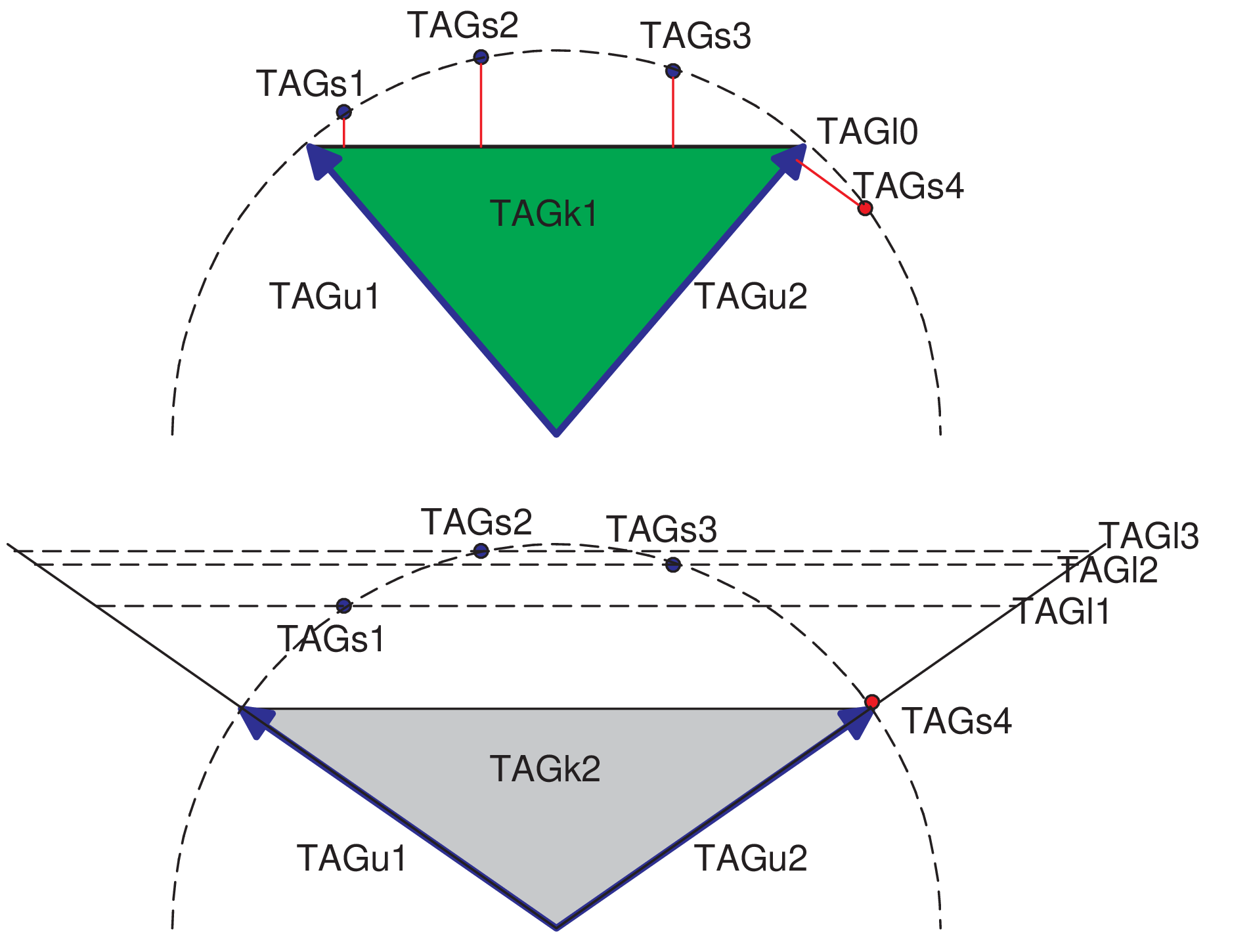
In our problem, we seek a cone which captures most of the training examples, i.e. the cone that encloses the conic hull of most training samples. In the SVM case, there are many possible hyperplanes that separates the samples without a controlled margin. Similarly, there is also a large number of polyhedral cones that can capture the training samples without further constraints. In fact, minimizing the empirical risk will tend to select the cone with larger solid angle so that the training examples will have small loss (see Fig. 2). In our case, the complexity is translated roughly to the size (volume) of the cone. The bigger cone will likely overfit (enclose) the noisy training samples and thus reduces generalization. Thus, we propose the following constraint to indirectly regularize the size of the cone

where $\mathbf{w}$ is the coefficients defined as in (1) and for simplicity we set $\lambda_{l}=1$. To see how this effectively controls $\mathcal{K}$, consider a 2D toy example in Fig. 2. If $\lambda_{u}=1$, the solution is the cone $\mathcal{K}_{1}$. In this case, the loss of the positive training examples (within the cone) is the distance from them to the simplex define over the basis vectors $\mathbf{u}_{1},\mathbf{u}_{2}$ (i.e. $\{\mathbf{z}:\mathbf{z}=\lambda\mathbf{u}_{1}+(1-\lambda)\mathbf{u}_{2},0\leq\lambda\leq 1\}$) and the loss of the negative training example is the distance to the cone. With the same training examples, if we let $\lambda_{u}>1$ then there exists a cone solution $\mathcal{K}_{2}$ such that all the losses are effectively zero. In particular, for each training example, there exists a corresponding $\|\mathbf{w}\|_{1}=\lambda$ such that the corresponding simplex $\{\mathbf{z}:\mathbf{z}=w_{1}\mathbf{u}_{1}+w_{2}\mathbf{u}_{2},w_{1}+w_{2}=\lambda\}$, passes all positive training examples.

Finally, we note that as the product $\mathbf{U}\mathbf{w}^{q_{i}}_{j}$ appears in the objective function and that both $\mathbf{U}$ and $\mathbf{w}^{q_{i}}_{j}$ are variables then there is a scaling ambiguity in the formulation. We suggest to address this scale ambiguity by considering the norm constraint $\|\mathbf{u}_{k}\|_{2}=c>0$ on the basis vectors.

In summary, the proposed formulation can be explicitly written as

We restrict our study on generalization bound from an algorithmic stability viewpoint, which is initially introduced in [2] and based on the concentration property of random variables. In the ranking context, generalization bounds for point-wise ranking / ordinal regression have been obtained [1, 8]. Recently, [13] show that the generalization bound result in [2] still holds in the ranking context. More specifically, we would like to study the variation of the expected query-level risk, defined as

where $L(\mathcal{K};q)$ denotes the expected query-level loss defined as

and ${P}_{\mathcal{Z}}$ denotes the probability distribution of the (ordered) document differences.

Following [2] and [13] we define the uniform leave-one-query-out document-pair-level stability as

where $\mathcal{K}_{S}$ and $\mathcal{K}_{S^{-i}}$ are respectively the polyhedral cones learned from the full training set and that without the $i$th query. As stated in [13], it can be easily shown the following query-level stability bounds by integration or average sum of the term on the left hand side in the above definition

Using the above query-level stability results and by considering $S_{q_{i}}$ as query-level samples, one can directly apply the result in [2] (see also [13]) to obtain the following generalization bound

As can be seen, the bound on the expected query-level risk depends on the stability. It is of practical interest to study the stability $\beta$ for the proposed algorithm. The following result shows that the change in the cone due to leaving one query out can provide an effective upper bound on the uniform stability $\beta$. For notational simplicity, we only consider the non-weighted version of the loss, as the weighted version is simply a scale of the bound by the maximum weight.

Proof. Following the proposed algorithm, we equivalently study the bound of

where the constraint set $\mathcal{C}=\{\mathbf{w}:\mathbf{w}\geq{\mathbf{0}},\lambda_{l}\leq\|\mathbf{w}\|_{1}\leq\lambda_{u}\}$. Without loss of generality, we can assume that

and the minima are attained at $\mathbf{w}$ and $\mathbf{w}^{-i}$ respectively. Due to the definition, it follows that

Expanding the term on the left, and using matrix norm inequalities, one obtains

where $\bm{\Delta}=\mathbf{U}-\mathbf{U}^{-i}$. The proof follows by the following facts

• •

  $\|\mathbf{U}\|\leq\sqrt{K}c$ due to each $\|\mathbf{u}_{k}\|_{2}\leq c$ and that $\|\mathbf{U}\|\leq\|\mathbf{U}\|_{F}$ where $\|\bullet\|_{F}$ denotes the Frobenius norm.

• •

  $\|\mathbf{w}\|_{2}^{2}\leq{\|\mathbf{w}\|_{1}^{2}}$ for $\mathbf{w}\geq{\mathbf{0}}$

• •

  $\|\mathbf{z}^{q}\|_{2}\leq\rho$ due to the normalization

and that $\|\bm{\Delta}\|\leq s_{\rm max}$ by definition.

It is more interesting to study the bound on $s_{\rm max}$. We conjecture that this will depend on the sample size as well as the nature of the proposed conic regularization. However, this is still an open question and such an analysis is beyond the scope of the current work.

We note importantly that as the stability bound can be made small by lowering $\lambda_{u}$. Doing so definitely improves stability at the cost of making the empirical risk large and hence the bias becomes significantly undesirable. In practice, it is important to select proper values of the parameters to provide optimal bias-variance trade-off. Next, we turn the discussion on practical implementation of the ideas, taking into account the large-scale nature of the problem.

Since the number of pairs may be large for typically real datasets, we do not want to store every $\mathbf{w}^{q}_{j}$. Instead, for each iteration, we perform a folding-in operation, in that we fix the basis $\mathbf{U}$, and estimate the coefficients $\mathbf{w}^{q}_{j}$. Since this is a convex problem, it is possible to apply the stochastic gradient (SG) method as shown in Algorithm 1. Note that we express the empirical risk as the function of only variable of interest when other variables are fixed for notational simplicity. In practice, we also need to check if the cone is proper and we find this is always satisfied.

Exponentiated Gradient (EG) [12] is an algorithm for estimating distribution-like parameters. Thus, Step 1a can be replaced by

For faster numerical computation (by avoiding the exponential), as shown in [12], this step can be approximated by

where the empirical risk $\hat{R}$ is parameterized in terms of $\hat{\mathbf{z}}^{q_{i}}_{j}=\mathbf{U}\mathbf{w}^{q_{i}}_{j}$. When the learning rate $\mu$ is sufficiently small, this update readily ensures the normalization of $\mathbf{w}^{q_{i}}_{j}$. The main difference between SG and EG is that, update in SG is additive, while it is multiplicative in EG.

Assume that the basis $\mathbf{U}=(\mathbf{u}_{1},\mathbf{u}_{2},...,\mathbf{u}_{K})$ has been learned during training. In testing, for each query, we are also given a set of feature vectors, and we need to compute a ranking function that outputs the appropriate positions of the vectors in the list.

Unlike the training data where the order of the pair $(l,m)$ is given, now this order information is missing. This breaks down the conic assumption, in that the difference of the two vectors is the non-negative combination of the basis vectors. Since the either preference orders can potentially be incorrect, we relax the constraint of the non-negative coefficients. The idea is that, if the order is correct, then the coefficients are mostly positive. On the other hand, if the order is incorrect, we should expect that the coefficients are mostly negative. The query-level prediction is proposed as shown in Algorithm 2. As this query-level prediction is performed over a query, it can address the shortcoming of logical discrepancy of document-level prediction in the pairwise approach.

We run the proposed algorithm on the latest and largest benchmark data LETOR 4.0. This has two data sets for supervised learning, namely MQ2007 (1700 queries) and MQ2008 (800 queries). Each returned document is assigned a integer-valued relevance score of $\{0,1,2\}$ where $0$ means that the document is irrelevant with respect to the query. For each query-document pair, a vector of $46$ features is pre-extracted, and available in the datasets. Example features include the term-frequency and the inverse document frequency in the body text, the title or the anchor text, as well as link-specific like the PageRank and the number of in-links. The data is split into a training set, a validation set and a test set. We normalize these features so that they are roughly distributed as Gaussian with zero means and unit standard deviations. During the folding-in step, the parameters $\mathbf{w}^{q}_{j}$ corresponding to pair $j$th of query $q$ are randomly initialized from the non-negative uniform distribution and then normalized so that $\|\mathbf{w}^{q}_{j}\|_{1}=1$. The basis vectors $\mathbf{u}_{k}$ are randomly initialized to satisfy the relaxed norm constraint. The learning rate is $\mu=0.001$ for the SG and $\mu=0.005$ for the EG. For normalization, we select $\alpha=1$ and $\rho=\sqrt{N}$ where $N$ is the number of features, and we set $c=2\rho$.

The two widely-used evaluation metrics employed are the Mean Average Precision (MAP) and the Normalized Discounted Cumulative Gain (NDCG). We use the evaluation scripts distributed with LETOR 4.0.

In the first experiment, we investigate the performance of the proposed method with respect to the number of basis vectors $K$. The result of this experiment on the MQ2007 dataset is shown in Fig. 3. We note an interesting observation that the performance is highest at about $K=10$ out of 46 dimensions of the original feature space. This seems to suggest that the idea of capturing an informative subspace using the cone makes sense on this dataset. Furthermore, the study on the eigenvalue distribution of the non-centralized ordered pairwise differences on on the MQ2007 dataset, as shown in Fig. 4, also reveals that this is about the dimension that can capture most of the data energy.

We then compare the proposed and recent base-line methods²² 2 from http://research.microsoft.com/en-us/um/beijing/projects/letor/letor4baseline.aspx in the literature and the results on the MQ2007 and MQ2008 datasets are shown in Table 1. The proposed ConeRank is studied with $K=10$ due to the previous experiment. We note that all methods tend to perform better on MQ2007 than MQ2008, which can be explained by the fact that the MQ2007 dataset is much larger than the other, and hence provides better training.

On the MQ2007 dataset, ConeRank compares favourably with other methods. For example, ConeRank-SG achieves the highest MAP score, whilst its NDCG score differs only less than 2% when compared with the best (RankSVM-struct). On the MQ2008 dataset, ConeRank still maintains within the 3% margin of the best methods on both MAP and NDCG metrics.

References

- [1] S. Agarwal, Lecture notes in artificial intelligence. Springer-Verlag, 2008, ch. Generalization bounds for some ordinal regression algorithms, pp. 7–21.
- [2] O. Bousquet and A. Elisseff, “Stability and generalization,” Journal of Machine Learning Research, pp. 499–526, 2002.
- [3] S. Boyd and L. Vandenberghe, Convex Optimization. Cambridge University Press, 2004.
- [4] C. Burges, T. Shaked, E. Renshaw, A. Lazier, M. Deeds, N. Hamilton, and G. Hullender, “Learning to rank using gradient descent,” in Proc. ICML, 2005.
- [5] Z. Cao, T. Qin, T. Liu, M. Tsai, and H. Li, “Learning to rank: from pairwise approach to listwise approach,” in Proc. ICML, 2007.
- [6] W. Chu and Z. Ghahramani, “Gaussian processes for ordinal regression,” Journal of Machine Learning Research, vol. 6, no. 1, p. 1019, 2006.
- [7] W. Cohen, R. Schapire, and Y. Singer, “Learning to order things,” J Artif Intell Res, vol. 10, pp. 243–270, 1999.
- [8] D. Cossock and T. Zhang, “Statistical analysis of Bayes optimal subset ranking,” IEEE Transactions on Information Theory, vol. 54, pp. 5140–5154, 2008.
- [9] Y. Freund, R. Iyer, R. Schapire, and Y. Singer, “An efficient boosting algorithm for combining preferences,” Journal of Machine Learning Research, vol. 4, no. 6, pp. 933–969, 2004.
- [10] R. Herbrich, T. Graepel, and K. Obermayer, “Large margin rank boundaries for ordinal regression,” in Proc. KDD, 2000.
- [11] T. Joachims, “Optimizing search engines using clickthrough data,” in Proc. KDD, 2002.
- [12] J. Kivinen and M. Warmuth, “Exponentiated gradient versus gradient descent for linear predictors,” Information and Computation, 1997.
- [13] Y. Lan, T.-Y. Liu, T. Quin, Z. Ma, and H. Li, “Query-level stability and generalization in learning to rank,” in Proc. ICML, 2008.
- [14] R. Plackett, “The analysis of permutations,” Applied Statistics, pp. 193–202, 1975.
- [15] B. Schölkopf and Smola, Learning with kernels. MIT Press, 2002.