Linear Latent Variable Models: The lava-package

Klaus Kähler Holst Email: k.k.holst@biostat.ku.dk Address: University of Copenhagen, Department of Biostatistics Esben Budtz-Jørgensen Email: e.budtz-joergensen@biostat.ku.dk Address: University of Copenhagen, Department of Biostatistics

Abstract

An R package for specifying and estimating linear latent variable models is presented. The philosophy of the implementation is to separate the model specification from the actual data, which leads to a dynamic and easy way of modeling complex hierarchical structures. Several advanced features are implemented including robust standard errors for clustered correlated data, multigroup analyses, non-linear parameter constraints, inference with incomplete data, maximum likelihood estimation with censored and binary observations, and instrumental variable estimators. In addition an extensive simulation interface covering a broad range of non-linear generalized structural equation models is described. The model and software are demonstrated in data of measurements of the serotonin transporter in the human brain.

Keywords:

latent variable model, maximum likelihood, multigroup analysis, structural equation model, R, serotonin, SERT

1 Introduction

Multivariate data are often modelled using random effects in order to account for correlation between measurements in the statistical analysis. The dominating model is the linear mixed effects model (Laird and Ware, 1982), which is available in most standard statistical software packages, e.g. SAS PROC MIXED and in R in the packages nlme (Pinheiro and Bates, 2000) and lme4 (Bates and Maechler, 2009) with the latter one also offering some support for generalized linear mixed models.

Another type of random effect model is the structural equation model (SEM) (Bollen, 1989), where the terminology latent variable often is used instead of random effects. While the mixed effect model and structural equation model have many aspects in common, the aim of a SEM analysis is typically to analyze the association between the latent variable, representing some process that is only partially observed, and some other variables (observed or latent). Thus, in SEMs focus is mainly on the latent variable, where one normally ascribes less interpretation to the random effects in a mixed effects model, which primarily serves as a way of capturing covariance between measurements. Because observed variables can be viewed as representations of underlying true variables SEMs offer a natural framework for handling measurement errors in study variables, and it often provides an efficient analysis of high dimensional data (Budtz-Jørgensen et al, 2003). The framework was pioneered by Jöreskog (Jöreskog, 1970) and since then it has been an active area of research with focus on relaxing linearity and distributional assumptions (Rabe-Hesketh et al, 2004).

SEMs have proven to be useful in many different fields of research. However, applications have been dominated by covariance structure analyses, and as residuals on the individual level are not available in this setup, model assessment has been based on more or less heuristic omnibus tests. The lack of profound model diagnostics have undoubtedly lead to several poor applications of SEMs (Steiger, 2001), and thus likely, however unjustified, giving the framework a somewhat bad reputation among groups of statisticians.

Several properitary software solutions are available for analyzing SEMs with some of the most popular being LISREL, SAS PROC CALIS, AMOS, EQS, Stata 12 sem, Stata gllamm (Rabe-Hesketh et al, 2004) and Mplus (Muthén and Muthén, 2007), where the last two programs stand-out because of their general modelling framework. Common for all these solutions is that they are difficult to extend and therefore possibilities for examination of new methodological ideas are limited. In part because details of many features of properitary software often remains hidden from the user. Implementations in an open-source environment such as R (R Development Core Team, 2010) directly address this problem. Currently two such solutions are available: the sem package (Fox, 2006; Fox, 2009) and the OpenMx package (Boker et al, 2011). While the former package is limited to standard covariance structure analysis, OpenMx offers sophisticated methods such as multiple group analysis, models for ordinal data and mixture models. The predecessor package Mx has been a popular for analyzing family data in epidemiological genetics and OpenMx will undoubtedly become an important tool in that field of research.

This paper presents the lava-package for statistical analysis in a very general modelling framework known as the Linear Latent Variable Model, which includes structural equation models and mixed models as important special cases. This model class also allows for non-linear effects of covariates and non-linear parameter constraints. The lava-package offers a superior user interface for specifying, altering and visualizing the model design. Models are specified independently of data using commands that are similar to standard regression modeling in R. In addition path diagrams can be generated to help give the user an overview of the assumptions specified. Further, the package gives access to an extensive simulation procedure which covers, but is not limited to, linear latent variable models. This tool will be extremely useful e.g. for understanding the biases caused by different types of model misspecification. The lava-package also includes sophisticated inferential methods such as multigroup analyses, robust standard errors for clustered correlated data, maximum likelihood based inference with data missing at random and inference for indirect and total effects. In addition advanced model diagnostic techniques for structural equation models (fitted in lava) are available via the gof-package (Holst, 2012), and extensions to models for censored and binary outcomes are available via the package lava.tobit (Holst, 2011) covered briefly in this article.

Modular programming has been a key concept during the software development thus making the process of extending the program (e.g. implementing new estimators, changing optimization routines etc.) easy, as exemplified by the above mentioned add-on packages.

Our hope is that the package will serve as a platform for testing, developing and sharing new ideas in the field of latent variable models.

2 Linear Latent Variable Models

We will define the Linear Latent Variable Model as the model defined by a Measurement part describing the responses $\bm{Y}_{i}=(Y_{i1},\ldots,Y_{ip})^{\prime}$ :

\displaystyle\begin{split}Y_{ij}&=\nu_{j}+\sum_{k=1}^{l}\lambda_{jk}\eta_{ik}+\sum_{r=1}^{q}\kappa_{jr}X_{ir}+\sum_{k=1}^{l}\delta_{jk}V_{ijk}\eta_{ik}+\epsilon_{ij},\end{split}

(1)

and a structural part describing the latent variables $\bm{\eta}_{i}=(\eta_{i1},\ldots,\eta_{il})^{\prime}$ :

\displaystyle\begin{split}\eta_{is}&=\alpha_{s}+\sum_{k=1}^{l}\beta_{sk}\eta_{ik}+\sum_{r=1}^{q}\gamma_{sr}X_{ir}+\sum_{k=1}^{l}\tau_{sk}W_{isk}\eta_{ik}+\zeta_{is},\end{split}

(2)

where $i=1,\ldots,n$ is the index of the sampling unit (e.g. individuals), $j=1,\ldots,p$ is the index of the observed variables (measurements or within cluster observations) and $s=1,\ldots,l$ is the index of the $l$ distinct latent variables. In a more compact matrix notation the model can be written as

\displaystyle\bm{Y}_{i}=\bm{\nu}+\bm{\Lambda}\bm{\eta}_{i}+\bm{K}\bm{X}_{i}+(\bm{\Delta}\odot\bm{V}_{i})\bm{\eta}_{i}+\bm{\epsilon}_{i},

(3)

\displaystyle\bm{\eta}_{i}=\bm{\alpha}+\bm{B}\bm{\eta}_{i}+\bm{\Gamma}\bm{X}_{i}+(\bm{T}\odot\bm{W}_{i})\bm{\eta}_{i}+\bm{\zeta}_{i},

(4)

where $\bm{\nu}\in\mathbb{R}^{p}$ and $\bm{\alpha}\in\mathbb{R}^{l}$ are intercepts, and $\bm{\Lambda},\bm{\Delta}\in\mathbb{R}^{p\times l}$ , $\bm{K}\in\mathbb{R}^{p\times q}$ , $\bm{\Gamma}\in\mathbb{R}^{l\times q}$ , $\bm{B},\bm{T}\in\mathbb{R}^{l\times l}$ are regression coefficient matrices (defining both fixed effects and random slopes), and $\bm{X}_{i}\in\mathbb{R}^{q},\bm{V}_{i}\in\mathbb{R}^{p\times l},\bm{W}_{i}\in\mathbb{R}^{l\times l}$ are covariates. The $\odot$ denotes the Schur product (element-wise multiplication). The residual terms follow multivariate normal distributions, $\bm{\epsilon}_{i}\sim{}$ $\mathcal{N}_{p}(0,\bm{\Sigma_{\epsilon}})$ and $\bm{\zeta}_{i}\sim\mathcal{N}(0,\bm{\Psi})$ , which typically are assumed to be independent.

Note that the terms including the covariates $\bm{V}_{i}$ and $\bm{W}_{i}$ define random slope components as in the Laird-Ware mixed model formulation and differentiates the LLVM from the usual SEM formulation (Sanchez et al, 2005). Many cases can however be modeled without such terms, resulting in a more computational efficient model formulation with constant variance between individuals. In the following we will therefore initially assume that the model is parameterized by some $\bm{\theta}$ defining the matrices

\displaystyle(\bm{\nu},\bm{\alpha},\bm{\Lambda},\bm{K},\bm{B},\bm{\Gamma},\bm{\Sigma_{\epsilon}},\bm{\Psi}),

(5)

with some restrictions on the parameter space to guarantee identification (obviously zeroes in the diagonal of $\bm{B}$ ), and possibly non-linear constraints between the different parameters. In Section 2.3 we will return to the general case, and demonstrate how to write up the model in atoms adapted to the case without any interaction terms. Note that we will allow non-linear constraints on the parameters between any of the elements in (5).

In the setup with $\bm{\Delta}=\bm{0}$ and $\bm{T}=\bm{0}$ it follows that the mean and variance of $\bm{Y}_{i}$ given the covariates are

\displaystyle\begin{split}\bm{\mu_{i}}(\bm{\theta})=\mathbb{E}(\bm{Y}_{i}\mid\bm{X}_{i})&=\bm{\nu}+\bm{\Lambda}(\bm{1}-\bm{B})^{-1}\bm{\alpha}\\ &\qquad+\left[\bm{\Lambda}(\bm{1}-\bm{B})^{-1}\bm{\Gamma}+\bm{K}\right]\bm{X_{i}},\end{split}

(6)

\displaystyle{\bm{\Sigma}}_{\bm{\theta}}=\mathbb{V}\text{ar}(\bm{Y}_{i}\mid\bm{X}_{i})

\displaystyle=\bm{\Lambda}(\bm{1}-\bm{B})^{-1}\bm{\Psi}(\bm{1}-\bm{B})^{-1}{}^{\prime}\bm{\Lambda}^{\prime}+\bm{\Sigma_{\epsilon}},

(7)

where the fundamental property of the normal distribution that the marginals also are normal is exploited. Inference about $\bm{\theta}$ can then be obtained by maximizing the corresponding likelihood (Bollen, 1989)

\displaystyle L(\bm{\theta};\bm{Y},\bm{X})\propto\prod_{i=1}^{n}\exp\left\{-\frac{1}{2}\left(\bm{Y_{i}}-\mu_{i}(\bm{\theta})\right)^{\prime}{\bm{\Sigma}}_{\bm{\theta}}^{-1}\left(\bm{Y_{i}}-\mu_{i}(\bm{\theta})\right)\right\}\left|{\bm{\Sigma}}_{\bm{\theta}}\right|^{-\tfrac{1}{2}}.

2.1 Implementation

From a mathematical and implementation-wise point of view it is convenient to supplement the model formulation with the equivalent Reticular Action Model (RAM) formulation (McArdle and McDonald, 1984; Fox, 2009), which have a direct connection with the underlying path diagram and also explicitly covers path analysis models. Let $\bm{U}$ be the stochastic vector including the latent variables, $\bm{\eta}$ ,

\displaystyle\bm{U}=(Z_{1},\ldots,Z_{p+q},\eta_{1},\ldots,\eta_{l})^{\prime}=(\bm{Z}^{\prime},\bm{\eta}^{\prime})^{\prime},

(8)

where $\bm{Z}=(Z_{1},\ldots,Z_{p+q})^{\prime}$ is the stochastic vector containing all observed variables $\bm{Z}=(Y_{1},\ldots,Y_{p},X_{1},\ldots,X_{q})^{\prime}$ . The RAM formulation states that

\displaystyle\bm{U}={\bm{v}}_{\bm{\theta}}+{\bm{A}}_{\bm{\theta}}\bm{U}+\bm{\epsilon},

(9)

where ${\bm{v}}_{\bm{\theta}}$ describes the intercepts, and $\epsilon$ is a residual term assumed to follow a zero-mean normal distribution with

\displaystyle\mathbb{V}\text{ar}(\bm{\epsilon})={\bm{P}}_{\bm{\theta}}.

(10)

Hence the model is completely specified by the matrices ${\bm{v}}_{\bm{\theta}}$ , ${\bm{P}}_{\bm{\theta}}$ and ${\bm{A}}_{\bm{\theta}}$ where the matrices generally are sparse, and the latter have zeros in the diagonal. In graph-terms the matrix ${\bm{A}}_{\bm{\theta}}$ represents the asymmetric paths whereas ${\bm{P}}_{\bm{\theta}}$ represent the symmetric paths.

Let $k$ be the total number of variables in the model (i.e. ${\bm{A}}_{\bm{\theta}}\in\mathbb{R}^{k\times k}$ ). We let $\bm{J}$ be the matrix that picks out the observed variables from $\bm{U}$ (see Section A), and define

\displaystyle{\bm{G}}_{\bm{\theta}}=\bm{J}(\bm{1}-{\bm{A}}_{\bm{\theta}})^{-1}.

(11)

Now it follows that

\displaystyle\mathbb{V}\text{ar}(\bm{Z})={\bm{\Omega}}_{\bm{\theta}}={\bm{G}}_{\bm{\theta}}{\bm{P}}_{\bm{\theta}}{\bm{G}}_{\bm{\theta}}^{\prime}.

(12)

and similarly the mean of the observed variables is then specified by the model structure as:

\displaystyle\mathbb{E}(\bm{Z})={\bm{\xi}}_{\bm{\theta}}={\bm{G}}_{\bm{\theta}}{\bm{v}}_{\bm{\theta}}.

(13)

The parameter $\bm{\theta}$ can then be estimated by maximizing the log-likelihood, $\ell$ , for the full data vector $\bm{Z}$

\displaystyle\widehat{\bm{\theta}}_{ML}=\operatorname{arg\,\max}_{\theta}\ell(\bm{\theta}\mid\bm{Z}=\bm{z}).

(14)

At a first glance this formulation seems restrictive in the sense that the covariates also have to be normally distributed. However, if we split the parameter vector into $\bm{\theta}=(\bm{\theta}_{1},\bm{\theta}_{2})$ , where $\bm{\theta}_{1}$ parameterizes the conditional distribution of $\bm{Y}$ given $\bm{X}$ and $\bm{\theta}_{2}$ are the mean and variance parameters of the covariates, then by Bayes formula the probability density for the joint distribution can be written as the product of the conditional density multiplied by the marginal density:

\displaystyle f_{\bm{\theta}_{1},\bm{\theta}_{2}}(\bm{y},\bm{x})=f_{\bm{\theta}_{1}}(\bm{y}\mid\bm{x})f_{\bm{\theta}_{2}}(\bm{x}).

(15)

It follows that maximum likelihood inference about the parameters $\bm{\theta}_{1}$ is independent of the model for the covariates, and hence finding the MLE of the conditional likelihood is equivalent to finding the MLE of the joint likelihood. If we fix $\bm{\theta}_{2}$ to the corresponding MLE, then the expected information agrees in the two models:

\displaystyle-\mathbb{E}\left(\frac{\partial^{2}\log f_{\bm{\theta}_{1}}(\bm{y}\mid\bm{x})}{\partial\bm{\theta}_{1}\partial\bm{\theta}_{1}^{\prime}}\right)=-\mathbb{E}\left(\frac{\partial^{2}\log f_{\bm{\theta}_{1},\widehat{\bm{\theta}}_{2}}(\bm{y},\bm{x})}{\partial\bm{\theta}_{1}\partial\bm{\theta}_{1}^{\prime}}\right).

(16)

An important advantage of the RAM formulation is that the empirical variance and mean are sufficient statistics for the parameters, thus giving the joint formulation a computational advantage over the conditional likelihood which requires explicit calculation of the likelihood contribution of each individual observation. In particular given the sufficient statistics, which are easily computed, the computational complexity in the RAM parameterization is independent of $n$ .

2.2 Inference - standard SEM

In the following we will describe inference under a priori non-linear constraints $\bm{\Omega}={\bm{\Omega}}_{\bm{\theta}}$ (twice differentiable w.r.t. $\bm{\theta}$ ). Letting $\widehat{\bm{\mu}}$ denote the empirical mean of the observed variables, we define

\displaystyle{\bm{W}}_{\bm{\theta}}=\left[\widehat{\bm{\mu}}-{\bm{\xi}}_{\bm{\theta}}\right]\left[\widehat{\bm{\mu}}-{\bm{\xi}}_{\bm{\theta}}\right]^{\prime}

(17)

and

\displaystyle{\bm{T}}_{\bm{\theta}}=\widehat{\bm{\Sigma}}+{\bm{W}}_{\bm{\theta}},

(18)

where $\widehat{\bm{\Sigma}}$ is the ML covariance matrix estimate (non-central estimate). We will exploit that

\displaystyle\begin{split}\sum_{i=1}^{n}(\bm{z}_{i}-{\bm{\xi}}_{\bm{\theta}})(\bm{z}_{i}-{\bm{\xi}}_{\bm{\theta}})^{\prime}&=\sum_{i=1}^{n}(\bm{z}_{i}-\widehat{\bm{\mu}}+\widehat{\bm{\mu}}-{\bm{\xi}}_{\bm{\theta}})(\bm{z}_{i}-\widehat{\bm{\mu}}+\widehat{\bm{\mu}}-{\bm{\xi}}_{\bm{\theta}})^{\prime}\\ &=n(\widehat{\bm{\Sigma}}+{\bm{W}}_{\bm{\theta}})+\\ &\qquad n\big[(\widehat{\bm{\mu}}-\widehat{\bm{\mu}})(\widehat{\bm{\mu}}-{\bm{\xi}}_{\bm{\theta}})^{\prime}+(\widehat{\bm{\mu}}-{\bm{\xi}}_{\bm{\theta}})(\widehat{\bm{\mu}}-\widehat{\bm{\mu}})^{\prime}\big]\\ &=n{\bm{T}}_{\bm{\theta}}.\end{split}

(19)

The complete log-likelihood then is given by

\displaystyle\begin{split}\ell(\bm{\theta}\mid\bm{z}_{1},\ldots,\bm{z}_{n})&=\sum_{i=1}^{n}\Big\{-\frac{k}{2}\log(2\pi)-\frac{1}{2}\log\left|{\bm{\Omega}}_{\bm{\theta}}\right|-\\ &\qquad\frac{1}{2}(\bm{z}_{i}-{\bm{\xi}}_{\bm{\theta}})^{\prime}{\bm{\Omega}}_{\bm{\theta}}^{-1}(\bm{z}_{i}-{\bm{\xi}}_{\bm{\theta}})\Big\}\\ &=-\frac{nk}{2}\log(2\pi)-\frac{n}{2}\log\left|{\bm{\Omega}}_{\bm{\theta}}\right|-\frac{n}{2}\tr\{{\bm{T}}_{\bm{\theta}}{\bm{\Omega}}_{\bm{\theta}}^{-1}\},\end{split}

(20)

with score

\displaystyle\begin{split}\frac{\partial\ell(\bm{\theta})}{\partial\bm{\theta}}&=\frac{n}{2}\left(\frac{\partial\operatorname{vec}{\bm{\Omega}}_{\bm{\theta}}}{\partial\bm{\theta}^{\prime}}\right)^{\prime}\operatorname{vec}\left[{\bm{\Omega}}_{\bm{\theta}}^{-1}{\bm{T}}_{\bm{\theta}}{\bm{\Omega}}_{\bm{\theta}}^{-1}\right]\\ &\qquad-\frac{n}{2}\left(\frac{\partial\operatorname{vec}{\bm{\Omega}}_{\bm{\theta}}}{\partial\bm{\theta}^{\prime}}\right)^{\prime}\operatorname{vec}\left[{\bm{\Omega}}_{\bm{\theta}}^{-1}\right]\\ &\qquad-\frac{n}{2}\left(\frac{\partial\operatorname{vec}{\bm{T}}_{\bm{\theta}}}{\partial\bm{\theta}^{\prime}}\right)^{\prime}\operatorname{vec}\left({\bm{\Omega}}_{\bm{\theta}}^{-1}\right),\end{split}

(21)

and the MLE is obtained by solving the corresponding score equation by Fisher scoring or a similar iterative procedure. See B for details w.r.t. expressions for the relevant matrix derivatives and information matrix.

In certain situations we may need to calculate conditional moments, for instance to calculate conditional residuals (model diagnostics) or the conditional likelihood given the covariates (likelihood ratio testing, model selection, etc.). Here we need to apply the selection matrix, $\bm{J}_{\bm{Y}}$ , that picks out the endogenous variables, $\bm{Y}$ , of $\bm{U}$ , and the cancellation matrix, $\bm{p}_{\bm{X}}$ , that sets all exogenous variables, $\bm{X}$ , of $\bm{U}$ to zero (see Section A). Notice we do not put any distributional assumptions on the exogenous variables.

Now

\displaystyle\bm{\mu_{i}}(\bm{\theta})=\mathbb{E}(\bm{Y}\mid\bm{X}=\bm{x})=\bm{J}_{\bm{Y}}(\bm{1}-{\bm{A}}_{\bm{\theta}})^{-1}(\bm{p}_{\bm{X}}{\bm{v}}_{\bm{\theta}}+\bm{v}_{\bm{x}}),

(22)

where $\bm{v}_{\bm{x}}$ is the $p$ -vector which is zero everywhere but on the index of the exogenous variables where it is set to $\bm{x}$ , and

\displaystyle{\bm{\Sigma}}_{\bm{\theta}}=\mathbb{V}\text{ar}(\bm{Y}\mid\bm{X})=\bm{J}_{\bm{Y}}(\bm{1}-{\bm{A}}_{\bm{\theta}})^{-1}(\bm{p}_{\bm{X}}{\bm{P}}_{\bm{\theta}}\bm{p}_{\bm{X}}^{\prime})(\bm{1}-{\bm{A}}_{\bm{\theta}})^{-1}{}^{\prime}\bm{J}_{\bm{Y}}^{\prime}.

(23)

2.3 Interactions with latent variables

Including interactions between covariates and random effects in the model, i.e. with non-zero $\bm{\Delta}$ and $\bm{T}$ in (3) and (4), we clearly loose the property of constant variance between individuals and the empirical mean and variance are therefore not sufficient. With $\bm{\Delta}$ and $\bm{T}$ consisting of ones in all entries, the marginal variance of $\bm{Y}_{i}$ , $\mathbb{V}\text{ar}(\bm{Y}_{i}\mid\bm{X}_{i},\bm{V}_{i},\bm{W}_{i})$ , will however take the same form as (7), exchanging $\bm{B}$ with

\displaystyle\bm{B}_{i}=\bm{B}+\bm{W_{i}},

(24)

and

\displaystyle\bm{\Lambda}_{i}=\bm{\Lambda}+\bm{Z_{i}},

(25)

hence the expression for the likelihood contribution and its derivatives of a single individual will take the same form as derived in B.

With free parameters in $\bm{\Delta}$ or $\bm{T}$ we can still adapt the model by adding one or more degenerate random effects. For instance, the term

\displaystyle\xi_{ij}=\delta_{jk}V_{ijk}\eta_{ik}+\epsilon_{ij}

(26)

where $\eta_{ik}$ and $\zeta_{ijk}$ follow normal distributions, can trivially be parameterized as the simultaneous equation

	$\displaystyle\xi_{ij}=\delta_{jk}\widetilde{\eta}_{ik}+\epsilon_{ij},$		(27)
	$\displaystyle\widetilde{\eta}_{ik}=V_{ijk}\eta_{ik}+0,$		(28)

hence the model is expanded to include a random effect with residual term with variance 0 with fixed slope parameter $Z_{ijk}$ , and the variance of the observed variables in such a model therefore takes the form as described above (24), i.e. $\bm{\Delta}=\bm{1}$ .

The possibility of including interactions with the random effects adds important flexibility to the model class for instance when modeling longitudinal data or to account for certain types of variance heterogeneity.

2.4 Non-linear effects

Allowing non-linear parameter constraints or non-linear effects of some covariates opens up for several interesting applications for instance in dose-response modeling. An important extension of the model framework is therefore to allow parametric non-linear functions $\phi^{(j)},j=1,\ldots,p$ and $\psi^{(s)},s=1,\dots,l$ of the covariates to enter the model:

\displaystyle\begin{split}Y_{ij}&=\nu_{j}+\sum_{k=1}^{l}\lambda_{jk}\eta_{ik}+\sum_{r=1}^{q}\kappa_{jr}X_{ir}+\sum_{k=1}^{l}\delta_{jk}V_{ijk}\eta_{ik}\\ &\qquad\qquad+\phi^{(j)}_{\bm{\gamma}_{1}}(X_{i1},\ldots,X_{iq})+\epsilon_{ij},\end{split}

(29)

and

\displaystyle\begin{split}\eta_{is}&=\alpha_{s}+\sum_{k=1}^{l}\beta_{sk}\eta_{ik}+\sum_{r=1}^{q}\gamma_{sr}X_{ir}+\sum_{k=1}^{l}\tau_{sk}W_{isk}\eta_{ik}\\ &\qquad\qquad+\psi^{(s)}_{\bm{\gamma}_{2}}(X_{i1},\ldots,X_{iq})+\zeta_{is}.\end{split}

(30)

Though we introduce non-linear effects in the model, we will still denote this model a Linear Latent Variable Model, as there are only linear effects of latent variables and endogenous variables in the model. Hence the observed data likelihood and its derivatives still have a closed form solution.

2.5 Multigroup analysis

A useful generalization of the model framework is the multigroup model, where we have several groups of data and specify a LLVM for each group. This naturally leads to the log-likelihood

\displaystyle\log L(\bm{\theta}\mid\bm{Y},\bm{X},\bm{V},\bm{W})=\sum_{g\in G}\log L_{g}(\bm{\theta}_{g}\mid\bm{Y}_{g},\bm{X}_{g},\bm{V}_{g},\bm{W}_{g})

(31)

where the intersection of the parameters $(\bm{\theta}_{g})_{\{g\in G\}}$ is not empty. Unbalanced designs and data with values missing at random (Little and Rubin, 2002) is naturally handled by this extension by forming groups from the different missing data patterns. Note that the additive structure of the log-likelihood makes the calculation of score functions and information matrices for the multigroup model explicitly available.

3 Model specification

The lava package aims to deliver a dynamic model specification experience in the sense that adding or removing model elements should be as easy as possible, and the model specification should be familiar to users accustomed to specifying models in for example glm in R. In order to achieve this we have designed a formal system for interactively specifying the complex hierarchical structure of a latent variable model. We believe this to be an important novel contribution, since the difficult specification of models in other languages often proves to be a significant obstacle.

The implementation relies on R (R Development Core Team, 2010) and the following packages all available from the Comprehensive R Archive Network (CRAN) : mvtnorm (Genz et al, 2009), graph (Gentleman et al, 2009), survival (Therneau and original R port by Thomas Lumley, 2009), numDeriv (Gilbert, 2009) and gof (Holst, 2012). The graphical system builds on graphviz (Gansner and North, 1999) and the R-package Rgraphviz (Gentry et al, 2009) (available from Bioconductor Gentleman et al (2004)).

	Function	Task
Primary functions
	lvm	Constructor of new model
	regression	Add regression association to model
	covariance	Add correlation between residuals terms
	intercept	Add intercept parameter
	constrain	Add non-linear covariate effects or
		parameter constraints
Secondary functions
	latent	Define latent variables in model
	addvar	Add variable to model
	parfix	Define equality constraints index of parameters
	parameter	Add a parameter name (for use with constrain)
	cancel	Remove previously defined associations
	kill	Remove variables from model

Table 1: Model building blocks

The specification of models in the lava-language is primarily achieved via the constructor function lvm and the two methods regression and covariance (see Table 1).

A new model object is initialized with the constructor lvm

> m1 <- lvm()which creates an empty lvm-object. Variables (or a multivariate regression formula as described below) can be fed to the lvm-function as arguments in order to control the order of entry in the graph layout. However, this is optional as variables automatically will be added during the process of defining the linear structure. A list of formulas is also valid as a shortcut for successive calls to regression (see below).

3.1 Specifying Linear Relationships

Linear associations between variables are specified via the member function regression taking the character vector arguments to and from. For convenience a replacement function, regression<-, is also available which in addition supports specification via the usual formula statements in R. As a simple example we will specify the following structural equation model with two measurement models

	$\displaystyle Y_{j}$	$\displaystyle=\mu_{j}+\lambda_{1j}U_{1}+\epsilon_{1j},$
	$\displaystyle Z_{j}$	$\displaystyle=\nu_{j}+\lambda_{2j}U_{2}+\epsilon_{2j},\quad j=1,\ldots,3,$

and structural model defined by

	$\displaystyle U_{1}$	$\displaystyle=\delta_{1}X_{1}+\delta_{2}X_{2}+\zeta_{1},$
	$\displaystyle U_{2}$	$\displaystyle=\beta_{1}X_{1}+\beta_{2}X_{2}+\zeta_{2},$

and $\mathbb{C}\text{ov}(\zeta_{1},\zeta_{2})\neq 0$ . The model is illustrated in the path diagram of Figure 1.

The following commands specifies a multivariate linear regression model with two covariates x1 and x2 and two outcomes u1 and u2

> m1 <- regression(m1, "u1", c("x1", "x2"))> regression(m1) <- u2 ˜ x1 + x2

In the following we will focus on the replacement functions and the formula specification as defined by the second line, but generally for all the available methods a standard function is available and arguments can be given as character vectors as above. A more compact call would simply be

> m1 <- lvm(c(u1, u2) ˜ x1 + x2)

Next, we define u1 and the u2 as a latent/unobserved variables using the latent-function:

> latent(m1) <- ˜u1 + u2Again arguments can generally be given as character vectors instead of a formulas. To remove the latent status from a variable we simply use the cancel=TRUE argument (latent(m1,cancel=TRUE) <- ...).

Next we define the measurement part of the model:

> regression(m1) <- c(y1, y2, y3) ˜ u1> regression(m1) <- c(z1, z2, z3) ˜ u2Covariance between residual terms can be specified using the replacement function covariance<- (or the function covariance) where the argument is a vector (or formula) of variables that are assumed to be pairwise correlated. In the current model specification, the residuals of the two latent variables are assumed to be conditionally independent given the covariates, and in order to define correlation between the residual terms of u1 and u2 we write

> covariance(m1) <- u1 ˜ u2which specifies $\mathbb{C}\text{ov}(\zeta_{1},\zeta_{2})\neq 0$ , thus completing the specification of the model defined by the path diagram in Figure 1. Note that the model is specified independently of any data. The model is linked to data when parameters are estimated using the estimate function (see Section 6). Here it is important that the manifest variable names used in the model specification corresponds to the variable names in the data-frame.

Refer to caption — Figure 1: Path diagram of the model m1 with correlation between residuals of the latent variables. Obtained with the command plot(m1). Following the convention of path diagrams observed variables are framed with rectangles whereas latent variables are framed with ellipses. Regression associations are depicted as one-headed arrows (parent=predictor, child=response) and covariance/correlations are shown as (dashed) double-headed arrows. For easier interpretation the following color-codes are used: exogenous:=light blue, endogenous:=orange, latent:=green.

Removal of associations or variables can be achieved with the cancel (and cancel<-) function which takes a character vector (or formula) as argument, removing any associations between all the variables in the vector. To remove the previously specified correlation and instead add a regression association between u1 and u2, we write

> cancel(m1) <- ˜u1 + u2> regression(m1) <- u2 ˜ u1Notice that the last regression call defining the association between u1 and u2 does not cancel the earlier defined predictors of u2. Hence the current definition says (see Figure 2) that

\displaystyle\mathbb{E}(U_{2}\mid U_{1},X_{1},X_{2})=\mu+\beta_{0}U_{1}+\beta_{1}X_{1}+\beta_{2}X_{2}

(32)

for some parameters $(\mu,\beta_{0},\beta_{1},\beta_{2})$ .

To completely remove one or more variables from the model we can use the kill<- function.

3.2 Constraining Parameters

Defining restrictions on some parameters is usually needed in order to obtain an identifiable model, and by default lava will automatically set reasonable restrictions when model parameters are estimated (see Section 6). Also, in situations where we need to test associations or use a priori knowledge in the model building, constraints on some parameters are needed. The lava package allows specification of completely general non-linear constraints on all parameters.

The most common type of constraints are identity constraints where one or more parameters are fixed to either a specific numerical value or to be equal to a common free parameter (equality constraints). For covariance and regression parameters (slope-parameters) the regression and covariance function can be used, and for the intercepts $\bm{\alpha}$ and $\bm{\nu}$ in (3-4), the intercept<- and intercept functions are used.

As an continuing example we will specify a new multivariate regression model with three outcomes, $(Y_{1},Y_{2},Y_{3})$ , and two predictors, $(X_{1},X_{2})$ :

\displaystyle Y_{i}=\beta_{i}X+\gamma_{i}Z+\epsilon_{i},i=1,\ldots,3

> mregr <- lvm(c(y1, y2, y3) ˜ x + z)

3.2.1 Constraining regression parameters

The restrictions of slope parameters can be accomplished with the regression function. For example fixing the slopes of $Y_{1}$ , $Y_{2}$ and $Y_{3}$ on $X$ to be identical, $b_{1}$ , and defining $Z$ as an offset (i.e. slope 1), can be achieved with the calls

> regression(mregr, c(y1, y2, y3) ˜ x) <- "b1"> regression(mregr, c(y1, y2, y3) ˜ z) <- 1To simultaneously define several different constraints a list can be given as the right-hand side argument

> regression(mregr, c(y1, y2) ˜ x + z) <- list(1, "a", 2, "b")All parameters for the first response on the covariates are given first, then for the second response, and so on. Hence in the above example we have

\displaystyle Y_{1}=X+aZ+\cdots\,\quad\text{ and }\quad Y_{2}=2X+bZ+\cdots

(33)

When defining constraints (intercepts, covariance or regression constraints) any missing associations will automatically be added to the model object. Hence the following call will add an extra level to the model, with a top-level response $W$ with identical effects of $Y_{1}$ , $Y_{2}$ and $Y_{3}$ (see Figure 3):

> regression(mregr, w ˜ y1 + y2 + y3) <- "beta"

To remove the constraints again (but not removing the associations) we simply fix to the logical constant NA:

> regression(mregr, w ˜ y1 + y2 + y3) <- NA

3.2.2 Constraining covariance parameters

Constraints on the covariance between residual terms are set with the covariance function, with a similar syntax. For example, to fix the covariance of the residuals terms of $Y_{1}$ and $Y_{2}$ to $0.5$ , and the variance of the residual term of $Y_{1}$ to a parameter v1:

> covariance(mregr, y1 ˜ y1 + y2) <- list("v1", 0.5)If we only need to constrain the variance parameters (i.e. not covariances) then the following syntax can be used

> covariance(mregr, ˜y1 + y2) <- "v"here setting the residual variance of $Y_{1}$ and $Y_{2}$ to be identical.

To fix the variance of the variables to different values, we simply give a list of the correct length as argument, e.g.

> covariance(mregr, ˜y1 + y2) <- list("v", 0.3)If we are interested in fixing only the covariance parameters (and not the diagonal) we can add the pairwise=TRUE argument. For instance to specify that the covariances between $Y_{1}$ , $Y_{2}$ , and $Y_{3}$ are the same, we can call

> covariance(mregr, ˜y1 + y2 + y3, pairwise = TRUE) <- "r1"thus specifying a compound-symmetry structure.

Finally a syntax like the one used by the regression-function can be used, such that

> covariance(mregr, c(y1, y2) ˜ y2 + y3) <- list(0.5, "r", "r0",+ 0.3)defines the following covariance structure between residual terms $\varepsilon_{1},\varepsilon_{2},\varepsilon_{3}$ corresponding to $Y_{1},Y_{2},Y_{3}$ (with the $\cdot$ denoting elements that are not affected by the call):

\displaystyle\mathbb{V}\text{ar}((\varepsilon_{1},\varepsilon_{2},\varepsilon_{3})^{\prime})=\begin{pmatrix}\cdot&0.5&r\\ 0.5&r_{0}&0.3\\ r&0.3&\cdot\end{pmatrix}

(34)

As with intercept and slope parameters, we can remove covariance constraints by fixing parameters to the value NA. We end up with a model as defined by the path-diagram in Figure 3.

3.2.3 Constraining intercepts

To fix the intercepts of the three outcomes to be identical, we can write

> intercept(mregr, ˜y1 + y2 + y3) <- "mu"Instead of a parameter name, mu, we could have chosen a numerical, say 0.

Notice that a character vector could also have been given instead of the formula. The value on the right can be given as a list, hence to fix the intercept of $Y_{1}$ and $Y_{2}$ to be identical and $Y_{3}$ to zero, we could call

> intercept(mregr, ˜y1 + y2 + y3) <- list("mu", "mu", 0)

3.3 Simultaneously specifying constraints on intercepts, slopes and variances

Using the formula syntax with the regression method it is possible to simultaneously specify constraints on intercept, regression and covariance parameters. A special function, f, can be used within the formula to specify the slope parameters, and further a pair of square brackets can be appended to each variable in the formula. Inside the square bracket the intercept of the variable can be defined, or alternatively both the intercept and residual variance separated by a colon. As an example we can specify

	$\displaystyle Y_{1}$	$\displaystyle=a+bU+\epsilon_{1},\quad\epsilon_{1}\sim\mathcal{N}(0,1),$
	$\displaystyle Y_{2}$	$\displaystyle=a+bU+\epsilon_{2},\quad\epsilon_{2}\sim\mathcal{N}(0,v),$
	$\displaystyle U$	$\displaystyle=b_{2}X+\zeta,$

using the square-bracket syntax:

> m2 <- lvm()> regression(m2) <- c(y1[a:1], y2[a:v]) ˜ f(u[0], b)> regression(m2) <- u ˜ f(x, b2)An equivalently even more compact model specification can be obtained using a list of formulas with the model initializer lvm, hence an equivalent way of specifying m2 would be

> m2 <- lvm(list(c(y1[a:1], y2[a:v]) ˜ f(u[0], b), u ˜ f(x, b2)))

If the index of the parameter is known (see the coef method below) the parfix method can also be used to simultaneous constrain parameters. For example to fix the parameters of a model m, at positions 1, 4 and 5 to the values a, a and 1, we can call

> parfix(m, c(1, 4, 5)) <- list("a", "a", 1)

3.4 Random slopes

Random slope effects (i.e. the matrices $\bm{V}_{i}$ and $\bm{W}_{i}$ ) can be defined by constraining the slope parameter of a latent variable to the name of a covariate. The covariate does not necessarily need to be added to the model explicitly, as the slope parameters are matched to the column names of the data.frame that is used during estimation (see Section 6).

In a standard structural equation model covariates enter the model in order to describe differences in the mean structure. Another question might be whether covariates can influence the variation in an outcome. In a situation where the variance depends on a covariate, the usual assumptions of variance homogeneity of the latent variables are not met and the model is not a SEM. In the LLVM this situation can be handled by defining a regression on the variance component using the random slope specification. Another important example is to use the random slopes to describe variation in longitudinal studies, and in combination with measurement models this allows us to formulate random regression models taking measurement error into account (see Figure 4).

3.5 Non-linear constraints and effects

Non-linear parameter constraints are defined using the constrain<- function. The syntax is

> constrain(m, formula) <- function(x) ...where m is the lvm-object, and the left-hand side in the formula specifies the parameter that is a (non-linear) function of the parameters or covariates defined by the right-hand side, and the function defines this association. The result of the function can optionally be given the attributes grad, defining the analytic gradient, and inv, defining a monotonic transformation (typically the inverse function) used in conjunction with confidence limit calculations (see Section 6 on Statistical Inference).

As an example we will define the model

\displaystyle Y_{ij}=\mu+b_{j}X_{i}+\epsilon_{ij},\quad j=1,2

(35)

with $\mathbb{C}\text{ov}(\varepsilon_{i1},\varepsilon_{i2})=0,\mathbb{V}\text{ar}(\epsilon_{ij})=v$ :

> mconstr <- lvm()> regression(mconstr, c(y1, y2) ˜ x) <- list("b1", "b2")> intercept(mconstr, ˜y1 + y2) <- "mu"> covariance(mconstr, ˜y1 + y2) <- "v"To restrict the variance-parameter to live on the positive real axis, we add the constraint

\displaystyle v=\exp(\alpha)

(36)

with

> constrain(mconstr, v ˜ alpha) <- expusing a log-link, and the parameter alpha (log-variance) is added to list of model parameters. In this example we do not set any attributes and numerical derivatives of the constraint will therefore be used (based on the package numDeriv) during estimation. Notice that constraints on the variance parameters can be set automatically by the estimate-function (see Section 6). For general domain constraints the function range.lvm can be used as the right-hand side argument, e.g. range.lvm(a=1,b=Inf) will bound the parameter to the interval $(1,\infty)$ .

Continuing the example, we could define the intercept, $\mu$ , to be the product of the two slope-parameters,

> constrain(mconstr, mu ˜ b1 + b2) <- prod

Constraints can be removed by letting the RHS be NULL (or NA)

> constrain(mconstr, "mu") <- NULL

If we instead wish to add a non-linear effect of $x$ on $y_{1}$ and $y_{2}$ :

\displaystyle Y_{ij}=\alpha+\Phi(\beta X_{ij})+b_{j}X_{ij}+\epsilon_{ij},\quad i=1,2

(37)

with $\Phi$ denoting the standard normal cumulative distribution function, we can make the call

> constrain(mconstr, mu ˜ alpha + beta + x) <- function(x) x[1] ++ pnorm(x[2] * x[3])

3.6 Complex models with feedback or co-existance of regression associations and covariance between residuals

The linear latent variable model framework in principle allows pathways going in both direction between two variables, i.e. feedback, and also simultaneous presence of both a regression association and covariance between residual terms of the same two variables. Note that both cases are different from a simple correlation between the residuals.

A simple example of an identified model is a illustrated in Figure 5, where the aim is to estimate the effect of $Y$ on $X$ while taking the unmeasured confounder $C$ into account. This can be achieved using an instrumental variable, $I$ , which by assumption must be (strongly) correlated with $X$ , independent with the confounder, and conditionally independent with the $Y$ given $X$ . We can model the inflation in covariance between $Y$ and $X$ using a correlation between their residual terms, which can be implemented as

> m <- lvm()> regression(m) <- y ˜ x> regression(m) <- x ˜ i> covariance(m) <- x ˜ y

4 Inspecting the model assumptions

Function	Task
plot	Plot the graph of the model
regression	Display parameter restrictions
intercept	Display parameter restrictions
covariance	Display parameter restrictions
exogenous	Extract (or define) exogenous variables (predictors)
endogenous	Extract set of endogenous variables (responses)
latent	Extract set of latent variables
manifest	Extract set of manifest (observed) variables
vars	Extract all variables
children	Extract children of a node
parents	Extract parents of a node
coef	Get list of parameters
constrain	Display non-linear constraints
path	Extract direct and indirect unidirectional
	pathways between nodes
subset	Extract sub-model
merge,%+%	Merge models

Table 2: Model inspection functions.

The philosophy of the lava package is to separate the model specification from the actual data, since examination of the model structure before actual estimation is often an important aspect of modelling within this class of statistical models. The lava package includes several functions as an aid to obtain an overview of the model assumptions (see Table 2). In general, the below described methods also applies for a lvmfit-object (see Section 6).

The plot-method (see Figure 1 and 3) visualizes the model using a path-diagram, i.e. a graph structure where linear (causal) associations are shown with directed edges and covariance between residuals are shown as bidirectional edges. Manifest variables are shown as rectangles and latent variables as ellipsoids. The parameter constraints can be added as labels on the edges with the argument labels=TRUE and variance parameters can be added with the argument diag=TRUE (see Figure 3). The plot-function will be explained in more details in Section 10.

Via the summary function, a complete overview of the model and (identity) parameter constraints can be obtained. Returning to the model mregr defined in Figure 3:

> summary(mregr)

Latent Variable Modelwith: 6 variables.Npar=11+2Regression parameters: y1 y2 y3 x z w y1 * y2 * y3 * x 1 2 b1 z a b 1 wCovariance parameters: y1 y2 y3 w y1 v 0.5 r y2 0.5 r0 0.3 y3 r 0.3 * w *Intercept parameters: y1 y2 y3 w mu mu 0 *Here the adjacency-matrix for the graph of all the unidirectional edges of the path-diagram can be read off under the title Regression parameters (i.e. slopes). Similarly the covariance structure of the residual terms and the intercept structure are shown. An empty element indicates that there is no direct association. A star indicates a free parameter and all other entries are either fixed numerical values or parameter names as defined by identity constraints during model specification. These three matrices can also be extracted via calls to regression, covariance or intercept.

The exogenous variables (covariates) of a lvm object can be identified with the exogenous function. Similarly a list of the endogenous (manifest) variables can be obtained with the function endogenous and the subset of these variables that do not predict other variables (top-level outcomes) can be shown by including the argument top=TRUE. In a similar way the observed and latent variables can be shown with manifest and latent. All variables of the model are listed with the vars function

> exogenous(mregr)

[1] "x" "z"

> endogenous(mregr, top = TRUE)

[1] "w"The children and parents functions extracts the children respectively the parents of one or several nodes in the unidirectional graph of the model, e.g.

> children(mregr, ˜x + y1)

[1] "y1" "y2" "y3" "w"

> parents(mregr, ˜w)

[1] "y1" "y2" "y3"The pathways from one variable to another can be viewed with the path function which returns a list of character vectors indicating the (causal) path

> path(mregr, w ˜ x)

[[1]][1] "x" "y1" "w"[[2]][1] "x" "y2" "w"[[3]][1] "x" "y3" "w"The function subset can be used to extract subsets of a model. To extract the upper level of the path analysis we call

> subset(mregr, ˜y1 + y2 + y3 + w)which keeps all parameter restrictions of the original model. Conversely, lvm models can be merged with the merge method (or using the operator syntax: m%++%m2).

To examine the parameters (and in particular their order) one can call the coef-function

> coef(mregr)

m1 m2 p1 p2 p3 p4 p5 p6 "y1" "w" "y1<-z" "y2<-z" "y3<-x" "w<-y1" "w<-y2" "w<-y3" p7 p8 p9 p10 p11"y1<->y1" "y2<->y2" "y3<->y3" "w<->w" "y1<->y3"where "<-" represents slope parameters (e.g. z on y1) and "<->" represents covariance (See also the describecoef function). With the argument labels=TRUE we can get the same vector but with all parameter labels substituted by their constraints

> coef(mregr, labels = TRUE)

m1 m2 p1 p2 p3 p4 p5 p6 "mu" "w" "a" "b" "b1" "w<-y1" "w<-y2" "w<-y3" p7 p8 p9 p10 p11 "v" "r0" "y3<->y3" "w<->w" "r"The non-linear parameter constraints or non-linear regression specifications can be shown with

> constrain(mconstr)

$vfunction (x) .Primitive("exp")attr(,"args")[1] "alpha"$mufunction (x)x[1] + pnorm(x[2] * x[3])attr(,"args")[1] "alpha" "beta" "x"

5 Simulation

Function	Task
sim	Simulation method for lvm-objects
functional,constrain	Introduce non-linearities in simulation
distribution	Change distribution and link of variables
heavytail	Define heavy tailed distribution of a variable
normal.lvm	Normal distribution
poisson.lvm	Poisson distribution
binomial.lvm	Binomial distribution
uniform.lvm	Uniform distribution
weibull.lvm	Weibull accelerated failure times

Table 3: Simulation methods.

Simulation is a major component of modern statistics, which allows us to experimentally study the properties of a statistical method under various alternatives and to verify (or reject) preliminary ideas. The lava package includes the sim method offering a convenient tool for performing simulation studies from very general models.

As an initial example we will create a data.frame with 100 observations from the structural equation model m1 defined in Section 3.1:

> mydata <- sim(m1, 100)The default parameter values are that all intercepts are 0, slope and residual variance parameters are 1, and covariance parameters are 0.5. To change the simulation parameters one can either fix the relevant parameters of the model to the desired numerical values as described in the previous section, or give the parameters as the argument p directly to the sim method. For instance the following two calls will both simulate 1000 observations from the model mregr with the default parameter values, except that the residual variance of $w$ is set to 2, the intercepts of $Y_{1}$ and $Y_{2}$ ( $\mu$ ) are set to 1, and $\beta=1.5$ (the slope of $Y_{1}$ on $W$ )

> d.mregr <- sim(mregr, 1000, p = c(mu = 2, beta = 1.5, `w<->w` = 2))> d.mregr2 <- sim(mregr, 1000, p = c(y1 = 2, `w<-y1` = 1.5, `w<->w` = 2))To simulate data with heavier tails than the normal distribution the heavytail method can be used. The following defines y1 and y2 to be realizations from an unstructured bivariate normal distribution $\mathcal{N}(\mu,\Sigma)$ :

> mhtail <- lvm()> covariance(mhtail) <- y1 ˜ y2We let $Y$ be a stochastic variable with this distribution, then the following call

> heavytail(mhtail, df = 3) <- ˜y1 + y2will allow us to draw simulations of y1 and y2 from the distribution of $\smash{Y_{j}(3/Q)^{0.5}}$ where $Q\sim\chi^{2}_{3}$ , i.e., leading to a multivariate $t$ -distribution with covariance matrix $\Sigma$ , mean $\mu$ , and $\nu=3$ degrees of freedom, described by the density

\displaystyle f(\bm{x}\mid\bm{\mu},\bm{\Sigma},\nu)=\frac{\Gamma((k+\nu)/2)}{\nu^{k/2}\Gamma(\nu/2)\Gamma(1/2)^{k}}\frac{\left|\bm{\Sigma}\right|^{-1/2}}{\left(1+\frac{1}{\nu}(\bm{x}-\bm{\mu})^{\prime}\Sigma^{-1}(\bm{x}-\bm{\mu})\right)^{(\nu+k)/2}}

(38)

where $k=2$ is the dimension. The same realization of $Q$ will be used on both y1 and y2 in the above code. To make simulations where a different realization of the $\chi^{2}$ -distribution is used for each outcome (leading to a star-shaped distribution), one simply has to make separate heavytail calls as in

> heavytail(mhtail, df = 3) <- ˜y1> heavytail(mhtail, df = 3) <- ˜y2The method can be used with different degrees of freedom for different variables in the model, and thus gives access to an easy way of simulating models with various degrees of outlier contamination.

To allow simulations from quite general models, two additional replacement functions are available, functional and distribution. The functional replacement function is used for defining (nonlinear) functional relationships between variables and has the syntax

  functional(x,to,from) <- value

where x is a lvm-object, from and to are predictor and outcome, respectively, and value is a real function describing the functional form. In the model mregr (Figure 3) we have

\displaystyle\mathbb{E}(Y_{3}|X,Z)=b_{1}X+Z

(39)

With the call

> functional(mregr, y3 ˜ x) <- function(x) xˆ2we can simulate from the model

\displaystyle\mathbb{E}(Y_{3}|X,Z)=b_{1}X^{2}+Z

(40)

with the coefficient $b_{1}$ defined by the earlier identity constraint. To define a more complex polynomial effect of $X$ we can make a copy of the predictor with the copy function and apply functional on the copy

> copy(mregr) <- x ˜ x2> regression(mregr, y3 ˜ x2) <- "b2"> functional(mregr, y3 ˜ x2) <- function(x) xˆ3leading to the mean-structure

\displaystyle\mathbb{E}(Y_{3}|X,Z)=b_{1}X^{2}+b_{2}X^{3}+Z

(41)

An alternative approach is to use the constrain function, e.g.

> functional(mregr, y3 ˜ x) <- NA> kill(mregr) <- ˜x2> intercept(mregr, ˜y3) <- "y3"> constrain(mregr, y3 ˜ b0 + b2 + b3 + x) <- function(x) x[1] ++ x[2] * x[4]ˆ2 + x[3] * x[4]ˆ3would define the model

\displaystyle\mathbb{E}(Y_{3}|X,Z)=b_{0}+b_{1}X+b_{2}X^{2}+b_{3}X^{3}+Z

(42)

The major difference between the two methods is that functional only has an impact on the sim method and not on the inferential methods, whereas constrain alters the model fitted by estimate (see Section 6).

The distribution replacement function is used for defining the link/distribution of variables, with syntax

  distribution(x,variable) <- value

where x is a lvm-object, variable is the variable to define the distribution of, and value is a function defining the random generator for variable taking the form

  function(n, mu, var)

where $n$ defines the number of samples, mu is the mean, and var is the variance as defined by the latent variable model. Some of the most common distributions have been predefined in the functions uniform.lvm, normal.lvm, binomial.lvm, poisson.lvm, weibull.lvm.

As an example we will define a simple hierarchical model structure (path analysis)

> msim <- lvm(t ˜ y + u + z)> regression(msim) <- y ˜ u + x + z> regression(msim) <- c(z, u) ˜ x

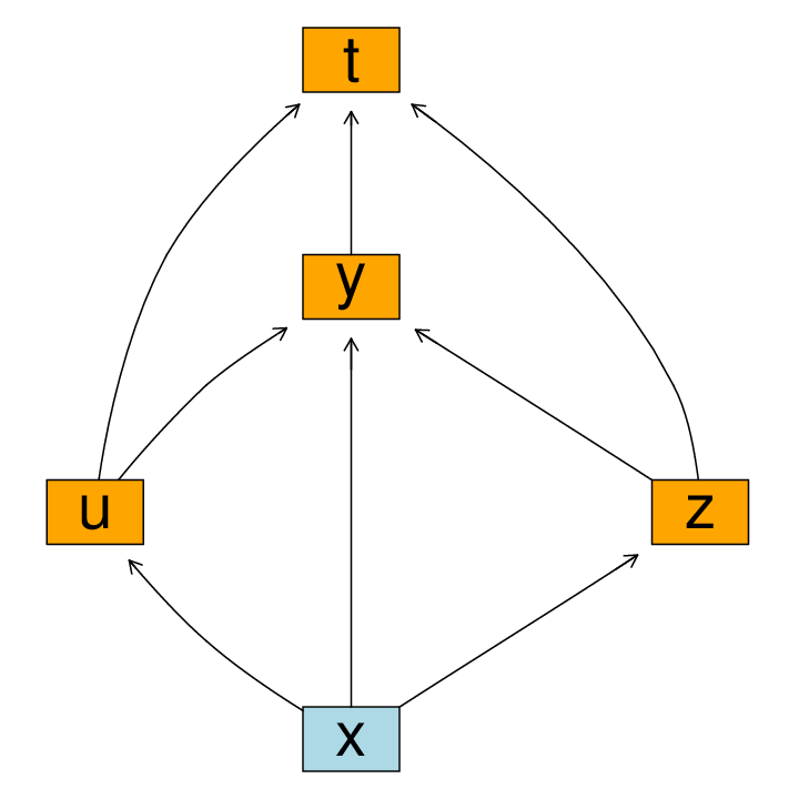
To change the distribution of $Y$ to a Bernoulli distribution we simply call

> distribution(msim, ˜y) <- binomial.lvm()The default link is logit

\displaystyle\mathbb{P}(Y=1\mid U,X,Z)=\frac{\exp(\beta_{0}+\beta_{1}X+\beta_{2}U+\beta_{3}Z)}{1+\exp(\beta_{0}+\beta_{1}X+\beta_{2}U+\beta_{3}Z)},

(43)

but a complementary log-log (cloglog) or probit link can be chosen via the link argument, e.g.

> distribution(msim, ˜y) <- binomial.lvm("probit")Similarly we can define the conditional distribution of $Z$ as Poisson

	$\displaystyle Z\sim pois(\mathbb{E}(Z\mid X)),$		(44)
	$\displaystyle\log(\mathbb{E}(Z\mid X))=\gamma_{0}+\gamma_{1}X,$		(45)

and the conditional distribution of $U$ as uniform

	$\displaystyle U=\lambda_{0}+\lambda_{1}X+\sqrt{\sigma_{U}^{2}}U_{0},$		(46)
	$\displaystyle U_{0}\sim unif(-1,1)\sqrt{3},$		(47)

and let $T$ follow a proportional hazards model with Weibull baseline with scale parameter 1.25 and shape parameter 2 (and no censoring)

\displaystyle\lambda(t)=\lambda_{0}^{Weibull}(1.25;2)\exp(-\alpha_{0}+\alpha_{1}U+\alpha_{2}Y+\alpha_{3}Z).

(48)

> distribution(msim, ˜z + u + t) <- list(poisson.lvm(), uniform.lvm(),+ weibull.lvm(1.25, 2, cens = Inf))The default simulation parameter values leads to intercepts $\beta_{0}=\lambda_{0}=\gamma_{0}=\alpha_{0}=0$ and all the remaining parameters are 1 (including the residual variance $\sigma_{U}^{2}$ ).

The default distribution of exogenous variables is the standard normal distribution, $X\sim\mathcal{N}(0,1)$ (and independence between the exogenous variables). It is also possible to let a variable be deterministic by simply assigning a list encapsulating the data:

  distribution(msim,~x) <- list(seq(0,1,length.out=100))

Obviously an error will occur if this variable definition differs in length from the number of samples to be drawn in the simulation.

Parameters can be altered in the same manner as endogenous variables (e.g. sim(msim, p=c(x=3,‘x<->x‘=2))), but they can also be fixed directly via the function distribution, e.g.

> distribution(msim, ˜x) <- binomial.lvm(p = 0.4)defines $X$ to be simulated from a Bernoulli-process ( $\mathbb{P}(X=1)=0.4$ ), with similar options for the other methods (e.g. poisson.lvm(lambda=2)).

For a lvmfit-object (see Section 6) the sim method by default simulates observations with the parameter vector p set equal to the estimated parameter vector and with the same number of observations as in the original data set. In this case the defaults causes the simulations to be drawn from the conditional distribution given the exogenous variables, hence the exogenous variables will be fixed at their original values (can be changed with the argument xfix=FALSE, in which case the covariates are simulated with mean and variance parameters set to the empirical mean and covariance).

6 Inference

Function	Task
estimate	Estimates parameters of lvm-objects
effects	Calculates direct and indirect effects
compare	Likelihood ratio, Wald and Score tests
gof	Goodness-of-fit measures
logLik	Extracts individual Likelihood values
information	Extracts information matrix
score	Extracts individual contribution to score
bootstrap	Non-parametric bootstrap
confint	Calculates confidence limits (Wald and profile)
constraints	Extracts non-linear parameter constraints
modelsearch	Model searching via score tests
equivalence	Finds empirically equivalent models

Table 4: Inferential tools.

Parameter estimation is achieved with the estimate-function which returns an object of class lvmfit. The syntax of the estimation procedure is:

  estimate(x, data, estimator, control=list(),
           missing, weight, cluster, fix, ...)

with the following arguments

x:: A lvm-object.
data:: data.frame with variables with the same names as the observed variables of the lvm object: manifest(x). The order of the variables is not relevant. Alternatively, for models where the empirical mean and variance are sufficient statistics (e.g. structural equation models), a list with the observed covariance matrix (S), the observed mean mu and the number of observations n can be passed as arguments, e.g.
data=list(S=cov(mydata),mu=colMeans(mydata),n=nrow(mydata)).
estimator:: Choice of estimator. Default is gaussian which is the MLE of the model defined by (3) and (4). See also Section 9.
control:: A list of parameters controlling the estimation and optimization procedures. See below for more details.
missing:: Logical variable. If FALSE (default) a complete case analysis is performed and else a full information likelihood analysis is conducted under a MAR assumption. Note that observations with missing covariates are excluded.
weight:: Optional weight matrix to be used by the estimation procedure defined by estimator (for multigroup analyses this should be a list of weights).
cluster:: Optional cluster variable identifying correlated groups of observations in the data set (for multigroup analyses this should be a list of cluster variables) to be used in the calculation of robust sandwich variance estimates.
fix:: Logical variable (defaults to TRUE). Care has to be taken when specifying a SEM in order to obtain an identifiable model. As a rule of thumb one regression coefficient in each measurement model should be fixed, e.g. to 1, and the intercept of one the indicator set to 0. By default the model is altered to fulfill these requirements unless fix=FALSE. Other parameterizations can be selected by setting the option param via the lava.options function. The above mentioned parameterization is obtained with lava.options(param="relative") and loading parameters and intercepts are then interpreted as differences compared to the reference indicator. Setting param="absolute" will result in a parameterization where the variance of the latent variables are fixed to 1 and the intercept to 0 if not already fixed at some other values. lava.options(param="hybrid") alters the model such that the intercept of latent variables are set to 0, and one factor loading in each measurement model is set to 1.

Calling lava.option(param="none") has the same effect as fix=FALSE (in which case the user has to manually define parameter constraints that guarantee model identification).

The optional control argument must be a list of parameters for the optimization procedure. The element method should be a string pointing to a generic optimizer conforming to the syntax of stats::nlminb (the default optimizer), i.e. accepting the objective function (e.g. the log likelihood), the gradient, the Hessian and control parameters. Setting method="nlminb0" will only use the objective function during optimization, where method= "nlminb1" also uses the gradient, and method="nlminb2" the Hessian as well. Defining method="NR" will use an alternative Newton-Raphson algorithm. Variance parameters are as default modeled using a $\log$ -link. This can be disabled by setting constrain=FALSE. Additional options like the number of iterations (iter.max), turning trace information on (trace=1), starter function (starterfun (a string pointing to a function generating starting values for the optimization), convergence tolerance (tol), reduction of step-size of the "NR" optimizer (gamma), etc. can also be defined (see the R help page of nlminb and estimate).

The control parameters can be set globally via the function lava.options. For instance to turn on the trace information of the optimizer as default in the current session, we would submit lava.options(trace=1).

We demonstrate the procedure in the ongoing example (see Figure 2) with the data obtained from the simulation in Section 5, using the hybrid parameterization:

> lava.options(param = "hybrid")> e <- estimate(m1, mydata)

> summary(e)

Latent variables: u1 u2Number of rows in data=100-------------------------------------------------- Estimate Std. Error Z value Pr(>|z|) std.xyMeasurements: y1<-u1 1.00000 0.85423 y2<-u1 0.85609 0.07774 11.01174 <1e-12 0.85902 y3<-u1 0.88990 0.08488 10.48415 <1e-12 0.83429 z1<-u2 1.00000 0.93812 z2<-u2 1.09038 0.05153 21.16099 <1e-12 0.96411 z3<-u2 1.02444 0.04998 20.49764 <1e-12 0.95745Regressions: u1<-x1 1.11118 0.13232 8.39775 <1e-12 0.61181 u1<-x2 0.96907 0.13392 7.23601 <1e-12 0.51159 u2<-u1 0.94651 0.17037 5.55569 2.765e-08 0.56706 u2<-x1 0.72832 0.21753 3.34815 0.0008135 0.24025 u2<-x2 1.05500 0.20428 5.16434 2.413e-07 0.33367Intercepts: u1 0.00000 0.00000 u2 0.00000 0.00000 y1 0.06805 0.15264 0.44582 0.6557 0.03110 y2 0.07461 0.12917 0.57759 0.5635 0.04005 y3 -0.08326 0.14244 -0.58453 0.5589 -0.04176 z1 0.07929 0.17709 0.44776 0.6543 0.02384 z2 0.07514 0.17400 0.43186 0.6658 0.02130 z3 0.07933 0.16811 0.47185 0.637 0.02376Residual Variances: u1 1.02921 0.23949 4.29753 0.29462 u2 0.87832 0.23741 3.69960 0.09024 y1 1.29397 0.23560 5.49234 0.27029 y2 0.90931 0.16777 5.41987 0.26209 y3 1.20812 0.21027 5.74543 0.30396 z1 1.32627 0.23349 5.68022 0.11993 z2 0.87762 0.19360 4.53323 0.07050 z3 0.92797 0.18768 4.94448 0.08328--------------------------------------------------Estimator: gaussian--------------------------------------------------Number of observations = 100 Log-Likelihood = -1010.407 BIC = 2167.944 AIC = 2066.814 log-Likelihood of model = -1010.407 log-Likelihood of saturated model = -1003.438 Chi-squared statistic: q = 13.93726 , df = 16 , P(Q>q) = 0.6033881--------------------------------------------------The parameter estimates in the output are divided into slope parameters belonging to the measurements part of the model (Measurements) (i.e. factor loadings), the structural part (Regressions) and the intercepts and residual (co)variances of the model. The summary method outputs all parameters of the model including the parameters that were fixed in contrast to the print method that only outputs the canonical parameters of the model. Notice that a regression parameter in each of the measurement models has been fixed to one in order to identify the model, and the slope parameter of $u_{2}$ on $u_{1}$ is therefore interpreted on the scale of $Y_{11}$ and $Y_{21}$ . The standardized coefficients in the last column are interpreted as the change in standard deviation of the outcome when increasing the predictor one standard deviation. These parameters can be used to compare effects of predictor variables measured on different scales. If non-linear constraints were defined then the relevant estimates and approximate standard errors will be shown in the last part of the summary output. These effects can also be extracted with the constraints function.

The p-values for the variance parameters are deliberately omitted from the output as the asymptotic distribution under the null is non-standard (derived in special-cases such as the random intercept model as an equal mixture of a $\chi^{2}_{1}$ -distribution and the Dirac measure in $0$ . Hence the naive p-values based on a $\chi^{2}_{1}$ -distribution will tend to be conservative). Different versions of the information matrix can be used, via the argument type $\in\{$ "E","hessian","outer","robust" $\}$ (expected information (default), minus the second derivative of the log-likelihood, outer product of the score, and the robust/sandwich variant (White, 1982)), to calculate the asymptotic standard errors of the parameters (see also the information function).

The last part of the output includes some fit criteria (Akaike and Bayesian) and the omnibus goodness-of-fit $\chi^{2}$ -test which is a likelihood ratio test of the current model against the saturated model structure. In the conditional model formulation, the least restrictive model allows covariance between residuals of all endogenous variables and the mean-vector $\bm{\mu}$ to be a general linear combination of all the covariates. In the unconditional model formulation (15), this corresponds to a completely free mean structure and a covariance $\bm{\Sigma}$ that can be any symmetric positive definite matrix. Clearly the maximum likelihood is attained at the sample mean and non-central empirical covariance matrix, $\bm{S}$ . Hence the log-likelihood of the saturated linear model is

\displaystyle-\frac{n}{2}\left(k\log(2\pi)+\log(\left|\bm{S}\right|)+\frac{n-1}{n}(p+q)\right).

(49)

This part of the output can also be obtained with the call

> gof(e, chisq = TRUE)

Number of observations = 100 Log-Likelihood = -1010.407 BIC = 2167.944 AIC = 2066.814 log-Likelihood of model = -1010.407 log-Likelihood of saturated model = -1003.438 Chi-squared statistic: q = 13.93726 , df = 16 , P(Q>q) = 0.6033881 RMSEA (90% CI): 0 (0;0.08127)rank(Information) = 23 (p=23)condition(Information) = 0.007602741||score||ˆ2 = 1.306582e-08Here the omnibus test gives a p-value of 0.60, thus indicating a reasonable agreement between the model implied and empirical covariance structure.

Byproducts of the maximum likelihood estimation such as the score, information and log-likelihood can be obtained with the functions score, information (see also vcov), and logLik. The individual contribution to score and log-likelihood are calculated with the argument indiv=TRUE. The methods also allow altering the parameter, data, weights and type of estimator (arguments p, data, weight and estimator). Predictions can be obtained via the predict method (and conditional residuals via residuals), where the latent variables are predicted by the conditional expectation given all manifest variables (the prediction can be based on conditioning on a subset of the manifest variables defined by the second argument of predict). For instance to estimate $\mathbb{E}(U_{1}\mid Y_{1},Y_{2},Y_{3},X_{1},X_{2})$ we can call

> u1hat <- predict(e, ˜y1 + y2 + y3)[, "u1"]Prediction of the residual terms can be obtained by setting the argument residual=TRUE.

> zeta1hat <- predict(e, ˜y1 + y2 + y3, residual = TRUE)[, "u1"]

Assessment of linearity and distributional assumptions can be based on examination of different residuals and their association with for example covariates in the model. We refer to the gof package (Holst, 2012) for residual based goodness-of-fit methods for structural equation models fitted with lava.

6.1 Direct and indirect effects

One of the strengths of the structural equation model framework is the possibility of decomposing the effects of a predictor into direct and indirect effects. In the model m1 (Figure 2) we have the following relations

$\displaystyle Z_{3}$	$\displaystyle=\lambda_{23}U_{2}+\epsilon_{23},$	(50)
$\displaystyle U_{2}$	$\displaystyle=\beta_{1}X_{1}+\beta_{2}X_{2}+\gamma U_{1}+\xi_{2},$	(51)
$\displaystyle U_{1}$	$\displaystyle=\delta_{1}X_{1}+\delta_{2}X_{2}+\xi_{1},$	(52)

and we wish to quantify the effect of $X_{1}$ on $Z_{3}$ . The direct effect is zero as $X_{1}$ is not present in (50). By substituting (51) and (52) into (50), it follows that

	$\displaystyle Z_{3}$	$\displaystyle=\beta_{1}\lambda_{23}X_{1}+\beta_{2}\lambda_{23}X_{2}+\beta_{2}\lambda_{23}X_{2}+\delta_{1}\gamma\lambda_{23}X_{1}$		(53)
		$\displaystyle\qquad+\delta_{2}\gamma\lambda_{23}X_{2}+\gamma\lambda_{23}\xi_{1}+\lambda_{23}\xi_{2}+\epsilon_{23}.$		(54)

Hence the total effect of $X_{1}$ is the sum of the two indirect effects $\beta_{1}\lambda_{23}$ and $\delta_{1}\gamma\lambda_{23}$ . The estimation uncertainty of this effect can be approximated by the delta method. In general the distribution of a product of estimators can be approximated in the following way. Let

\displaystyle f(\widehat{\bm{\beta}})=f(\widehat{\beta}_{1},\ldots,\widehat{\beta}_{k})=\prod_{i=1}^{k}\widehat{\beta}_{i},

(55)

where the estimated parameters $\widehat{\bm{\beta}}$ are asymptotically normally distributed with covariance matrix $\bm{\Sigma}_{\bm{\beta}}$ . Now

\displaystyle\nabla f(\bm{\beta})=\begin{pmatrix}\prod_{i\neq 1}\beta_{i}\\ \vdots\\ \prod_{i\neq k}\beta_{i}\end{pmatrix}

(56)

and

\displaystyle\sqrt{n}\Big(f(\widehat{\bm{\beta}})-f(\bm{\beta}_{0})\Big)\overset{\mathcal{D}}{\longrightarrow}\mathcal{N}\Big(0,\,\nabla f(\widehat{\bm{\beta}})^{\prime}\bm{\Sigma}_{\widehat{\bm{\beta}}}\nabla f(\widehat{\bm{\beta}})\Big)

(57)

The approximate distribution of linear combinations of products is obtained by straightforward calculations (i.e. $\nabla f_{1}+\nabla f_{2}$ ).

The effects function can be used to estimate the (direct and indirect) effect of one variable on another together with approximate standard errors, e.g.

> (f <- effects(e, z3 ˜ x1))

Total effect of ’x1’ on ’z3’:1.823569 (Approx. Std.Err = 0.1524713)Direct effect of ’x1’ on ’z3’:0 (Approx. Std.Err = NA)Indirect effects:Effect of ’x1’ via x1->u1->u2->z3:1.077448 (Approx. Std.Err = 0.2170743)Effect of ’x1’ via x1->u2->z3:0.7461208 (Approx. Std.Err = 0.222262)

> coef(f)

Estimate Std.Err z value Pr(>|z|)Total 1.8235689 0.1524713 11.960083 0.000000e+00Direct 0.0000000 NA NA NAz3<-u2<-u1<-x1 1.0774481 0.2170743 4.963498 6.923458e-07z3<-u2<-x1 0.7461208 0.2222620 3.356943 7.880941e-04

6.2 Hypothesis testing

Next we estimate the parameters of two nested models where we have restricted all factor loadings to 1 and in addition removed the effect from $U_{1}$ to $U_{2}$

> m1a <- m1> regression(m1a, c(z1, z2, z3) ˜ u2) <- 1> regression(m1a, c(y1, y2, y3) ˜ u1) <- 1> m1b <- m1a> cancel(m1b) <- u2 ˜ u1> ea <- estimate(m1a, mydata)> eb <- estimate(m1b, mydata)

6.2.1 Likelihood Ratio Test

For nested models, $\mathcal{M}_{1}\subseteq\mathcal{M}_{2}$ , the natural test is the likelihood ratio test (LRT)

\displaystyle-2\left[\log L_{1}(\widehat{\bm{\theta}}_{1})-\log L_{2}(\widehat{\bm{\theta}}_{2})\right]\overset{\text{approx.}}{\sim}\chi^{2}_{\Delta df}.

(58)

For non-nested models, one choice is the Akaike’s Information Criterion (AIC) favoring models with low values of

\displaystyle AIC=-2\log(L)+2n_{\text{par}},

(59)

where $n_{\text{par}}$ is the number of parameters in the model (implemented in the AIC function), or the Bayesian Information Criterion

\displaystyle BIC=-2\log(L)+n_{\text{par}}\log(N),

(60)

where $N$ denotes the total number of observations (Raftery, 1993), i.e. the number of endogenous variables times the number of individuals.

Successive LRT between nested models can be calculated with

> (LRT1 <- compare(e, ea, eb))

[[1]]Likelihood ratio testdata:chisq = 6.6542, df = 4, p-value = 0.1553sample estimates:log likelihood (model 1) log likelihood (model 2) -1010.407 -1013.734[[2]]Likelihood ratio testdata:chisq = 33.9868, df = 1, p-value = 5.549e-09sample estimates:log likelihood (model 1) log likelihood (model 2) -1013.734 -1030.728Hence we accept the hypothesis that all factor loadings are equal (the model m1a) but reject the hypothesis that the two latent variables $U_{1}$ and $U_{2}$ are conditional independent given the covariates.

6.2.2 Wald Test

The compare method can also deal with hypothesis testing via Wald or Score tests. The hypothesis

\displaystyle H_{0}\colon\bm{\beta}=\bm{\beta}_{0}

(61)

for a subset, $\bm{\beta}$ , of all the parameters, can be tested with a Wald test using the par and null arguments (the latter defaults to 0), for instance to test if all loading parameters are 1 (equivalent to the LRT of m1 against m1a), we can write

> (W1 <- compare(e, par = c("y2<-u1", "y3<-u1", "z2<-u2", "z3<-u2"),+ null = rep(1, 4)))

Wald testdata:chisq = 7.2687, df = 4, p-value = 0.1223For a general estimable contrast $\bm{C}$ , we can also test the hypothesis

\displaystyle H_{0}\colon\bm{C}\bm{\beta}=\widetilde{\bm{\beta}}_{0},

(62)

where $\bm{C}$ is matrix (or vector) with the same number of columns as the number of parameters, or alternatively a sub-matrix with column names given by parameter names (implicitly assuming that omitted columns are zero), leading to the test statistic

\displaystyle(\bm{C}\widehat{\bm{\beta}}-\widetilde{\bm{\beta}}_{0})^{\prime}(\bm{C}\bm{\Sigma}_{\widehat{\bm{\beta}}}\bm{C}^{\prime})^{-1}(\bm{C}\widehat{\bm{\beta}}-\widetilde{\bm{\beta}}_{0})\sim\chi^{2}_{\rank(\bm{C)}}

(63)

The covariance matrix $\bm{\Sigma}_{\widehat{\bm{\beta}}}$ will by default be the variance matrix as defined by the chosen estimator (for the linear gaussian models, estimator="gaussian", this is the inverse of the expected information), but it can optionally be given as the argument Sigma, e.g. to use a robust variance estimate (see information method).

To test whether all the intercepts of the outcomes sum to zero, we can write

> C <- rep(1, 6)> names(C) <- endogenous(m1)> (W2 <- compare(e, contrast = C))

Wald testdata:chisq = 0.1769, df = 1, p-value = 0.6741hence we accept the hypothesis of equal intercepts.

6.2.3 Score Test

With the scoretest argument we can conduct Score tests. Letting $\widetilde{\bm{\theta}}$ be the parameter belonging to the less restrictive model $\mathcal{M}_{2}$ , which is equal to $\widehat{\bm{\theta}}_{1}$ , the MLE of the restrictive model $\mathcal{M}_{1}$ , for all the parameters shared by $\mathcal{M}_{2}$ and zero elsewhere. The test statistic is then given by

\displaystyle S=\mathcal{S}_{2}(\widetilde{\bm{\theta}})^{\prime}\mathcal{I}_{2}^{-1}(\widetilde{\bm{\theta}})\mathcal{S}_{2}(\widetilde{\bm{\theta}})

(64)

with approximate $\smash{\chi^{2}_{\Delta df}}$ -distribution under the null, where $\mathcal{S}_{2}$ and $\mathcal{I}_{2}$ are the score and information matrix of model $\mathcal{M}_{2}$ .

We will test whether adding correlation between the residuals terms of $Z_{3}$ and $Z_{2}$ significantly improves the model fit:

> (S1 <- compare(e, scoretest = z3 ˜ z2))

Score testdata: z3 ˜ z2chisq = 0.1186, df = 1, p-value = 0.7306which does not indicate evidence against the conditional independence assumption.

Similarly we can test the statistical significance of simultaneously adding two extra correlation parameters:

> (S2 <- compare(e, scoretest = c(z3 ˜ z2, z1 ˜ z2)))

Score testdata: z3 ˜ z2 z1 ˜ z2chisq = 2.03, df = 2, p-value = 0.3624

6.2.4 Model searching with the Score test

An advantage of the Score test over the LRT is that the MLE is only needed in the more restrictive model making it an ideal instrument for model searching, in order to check that important aspects of the covariance structure has not been neglected in the model specification. The modelsearch function can be used to examine all one-parameter extensions of the model. The following call give the 5 most significant one-parameter extensions

> print(ms <- modelsearch(e), tail = 5)

Score: S P(S>s) Index holm BH 2.024 0.1549 u2<->y1 1 0.9031 2.124 0.145 y1<->z1 1 0.9031 2.283 0.1308 y1<->y2 1 0.9031 2.892 0.08904 y2<->z2 1 0.9031 4.207 0.04025 y2<->z1 1 0.9031As expected we do not see any significant improvements of the model among the 5 most significant Score tests (with the first and second column being the test statistic and corresponding p-value, and the last two columns being the p-values adjusted by the Bonferroni-Holm procedure to control the overall Type I error (Holm, 1979), and q-values of the Benjamini-Hochberg procedure controlling the FDR). Similarly, the most important $k$ -parameter extensions to the model, can be examined with the argument k, but the number of models to search through will increase dramatically with $k$ .

6.3 Model equivalence

A challenge in multivariate modeling is the problem of equivalent models, where two different parameterizations leads to identical model fit (likelihood) for all data sets. Hence without strong a priori knowledge of the model structure, e.g. based on other scientific evidence, the interpretation of model parameters must be made cautiously. Formal proofs of model equivalence can be difficult (Bollen, 1989). To identify candidates of equivalent models we suggest using the Score test. The idea is to study all one-parameter extensions of a given model using the score test. Two models are said to be empirically equivalent if the score tests agree. This can be achieved with the equivalence function. Two variables of the model are chosen, which not necessarily are defined as being directly related in the model structure. The score function for the model including covariance between the residuals of the two selected variables is then compared with score functions of models omitting this association, but with the same number of parameters.

As a simple example we will investigate the structural equation model in the path diagram of the left panel of Figure 7

> mEq <- lvm(list(c(y1, y2, y3) ˜ u, u ˜ x))> latent(mEq) <- ˜u> covariance(mEq) <- y1 ˜ y2> dEq <- sim(mEq, 100)> est.mEq <- estimate(mEq, dEq)

Below we are examining whether the inclusion of a residual correlation between $Y_{1}$ and $Y_{2}$ has any equivalent formulations

> (Eq <- equivalence(est.mEq, y1 ˜ y2))In fact, an equivalent model is defined by instead adding a direct effect of $X$ on $Y_{3}$ (see Figure 7).

0) y1<->y2 (10.31)Empirical equivalent models: 1) y3<->x (10.31)Candidates for model improvement: none

6.4 Confidence limits

Wald confidence limits can be created using the method confint. However, for some parameters better coverage can be achieved with alternative methods. One method is the non-parametric bootstrap which can be calculated with the function bootstrap. The bootstrap is a computational intensive method, and parallel computation can be done by registering a foreach (REvolution Computing, 2009) parallel adaptor. In this example we will compute the bootstrap in parallel using the parallel and doParallel packages distributing the bootstrap computations across the available CPU cores

> library(doParallel)> registerDoParallel()> (B <- bootstrap(e, 500))

Non-parametric bootstrap statistics (R=500): Estimate Bias Std.Err 2.5 % 97.5 %y1 0.08467677 1.662669e-02 0.15922250 -0.2417240 0.3787349y2 0.07691911 2.312410e-03 0.12146566 -0.1457868 0.3101638y3 -0.07196788 1.129167e-02 0.13941055 -0.3536971 0.2112750z1 0.08407469 4.780799e-03 0.18185690 -0.2799668 0.4421753z2 0.08527725 1.013330e-02 0.17283489 -0.2966441 0.3995207z3 0.09493044 1.560519e-02 0.17017286 -0.2081544 0.4407723u1<-x1 1.11860351 7.421090e-03 0.15172036 0.8141602 1.4084714u1<-x2 0.96908130 1.303164e-05 0.15096572 0.6741721 1.2717508u2<-u1 0.96947448 2.296893e-02 0.16712619 0.6754198 1.3478912u2<-x1 0.69630433 -3.201448e-02 0.23181926 0.1494670 1.0941781u2<-x2 1.02390307 -3.109418e-02 0.20826885 0.5773626 1.4170756y2<-u1 0.85971870 3.632407e-03 0.10370758 0.6779335 1.0642511y3<-u1 0.89440961 4.508961e-03 0.08414864 0.7388379 1.0566335z2<-u2 1.09661468 6.232894e-03 0.05341720 0.9971030 1.2131320z3<-u2 1.02856111 4.118107e-03 0.04733460 0.9419200 1.1232677u1<->u1 0.99249288 -3.671648e-02 0.27738180 0.5390826 1.5590308u2<->u2 0.81896688 -5.935355e-02 0.26481969 0.3523745 1.3589482y1<->y1 1.28947917 -4.494201e-03 0.26570998 0.8302451 1.8369823y2<->y2 0.89753510 -1.177998e-02 0.17311848 0.5861767 1.2511752y3<->y3 1.18530385 -2.281194e-02 0.18883960 0.8092845 1.5525326z1<->z1 1.30673170 -1.953404e-02 0.21030950 0.9245536 1.7315556z2<->z2 0.84766364 -2.995799e-02 0.17431201 0.4971759 1.1894273z3<->z3 0.92206325 -5.906032e-03 0.18632891 0.5572348 1.3095068To bootstrap other statistics a user-defined function can be supplied as the argument fun. A parametric bootstrap can be computed setting the argument parametric=TRUE and setting the argument p to parameter values of the null model from which to simulate from. The parallel computation functionality can be disabled via the call lava.options(parallel=FALSE).

As an alternative to the resample-based approach, we can also calculate the confidence limits based on the profile likelihood:

> (ci <- confint(e, profile = TRUE, parm = "u2<-u1", level = 0.95))

2.5 % 97.5 %u2<-u1 0.6392854 1.332559where the parameter of interest can be given as the index or label name.

A third option is to use a variance stabilizing transform of the parameter. As an example we will calculate the confidence limits of the partial correlation (or conditional correlation) between two outcomes $Y_{1}$ and $Y_{2}$ given covariates $\bm{X}$ . Hence we assume that

\displaystyle Y_{i}=\bm{\beta}_{i}^{\prime}\bm{X}+\varepsilon_{i},\quad i=1,2

(65)

and aim to estimate the correlation, $\rho$ , between $\varepsilon_{1}$ and $\varepsilon_{2}$ .

We define this model with a single covariate and simulate some observations and find the corresponding MLE:

> m <- lvm(c(y1, y2) ˜ x)> covariance(m, y1 ˜ y2) <- "C"> covariance(m, ˜y1 + y2) <- list("v1", "v2")> d <- sim(m, 100)> e.pcor <- estimate(m, d)Note with the default parameter values the correlation between $\epsilon_{1}$ and $\epsilon_{2}$ is 0.5. Next we define the correlation parameter using a non-linear parameter constraint and obtain the estimate with confidence limits based on the delta method

> constrain(e.pcor, rho ˜ C + v1 + v2) <- function(x) x[1]/(x[2] *+ x[3])ˆ0.5> constraints(e.pcor)

Estimate Std. Error Z value Pr(>|z|) 2.5% 97.5%rho 0.4449733 0.08019988 5.548303 2.884553e-08 0.2877844 0.6021621Near the boundary of the parameter space these limits will tend to perform poorly and a better approach is to apply the variance stabilizing $\arctanh$ transform (Fishers z-transform):

\displaystyle\mathcal{Z}\colon\rho{\mapsto}\frac{1}{2}\log\left(\frac{1+\rho}{1-\rho}\right)

(66)

Here we also supply the analytical gradient (optional) calculated with the chain-rule and in addition we set the attribute inv defining the inverse transformation, thus giving us the confidence limits on original correlation scale:

> constrain(e.pcor, z ˜ C + v1 + v2) <- function(x) {+ f <- function(p) p[1]/sqrt(p[2] * p[3])+ res <- atanh(f(x))+ df <- function(p) c(1/sqrt(p[2] * p[3]), -f(p)/(2 * p[2]),+ -f(p)/(2 * p[3]))+ datanh <- function(r) 1/(1 - rˆ2)+ attributes(res)$grad <- function(p) datanh(f(p)) * df(p)+ attributes(res)$inv <- tanh+ return(res)+ }> constraints(e.pcor)

Estimate Std. Error Z value Pr(>|z|) 2.5% 97.5%rho 0.4449733 0.08019988 5.548303 2.884553e-08 0.2877844 0.6021621z 0.4784149 0.10000000 4.784149 1.717133e-06 0.2824185 0.6744113inv(z) 0.4449733 NA NA NA 0.2751420 0.5878741In fact $\sqrt{n}\mathcal{Z}(\widehat{\rho}_{n})\overset{\mathcal{D}}{\rightarrow}\mathcal{N}(0,1)$ as $n\to\infty$ (Lehmann and Romano, 2005). Note that the correlation method calculates the correlation coefficients of a lvmfit object in a more elegant way and with a slightly more precise variance estimate (Hotelling, 1953) (see also the partialcor function).

7 Multigroup models

Multigroup analysis (31) can be used to combine different models linked via some shared parameters. Among other things this extension can be useful in testing general hypotheses of linear interactions, and the lava package supports this generalization via the estimate-function taking a list of lvm-objects and a list of data.frame’s as arguments and returning an object of class multigroupfit:

> estimate(list(m1, m2, m3, ...), list(d1, d2, d3, ...), ...)The list of lvm objects can optionally be named, as in the example below, to enhance the output. Parameters that are shared across the models m1,m2,m3, $\ldots$ will be also be shared in the multigroup analysis, whereas all other parameters will be estimated independently between the groups. In many applications the first argument will therefore be repetitions of the same lvm-object. Note, that when the different datasets are defined from a single data.frame using a grouping variable, the function split can be applied to define the second argument. A typical multigroup analysis call will therefore resemble

> estimate(rep(m, n), split(d, d$x))where the data-frame d here is split into a list defined from the variable d$x (with, in this case, n distinct values).

As an example we will create two nearly identical lvm-objects describing simple factor models (see Figure 8):

> mg1 <- lvm()> regression(mg1, Y1 ˜ H) <- 1> intercept(mg1, ˜Y1) <- 0> regression(mg1) <- c(Y2, Y3) ˜ H> regression(mg1) <- H ˜ E> latent(mg1) <- ˜H> mg1 <- baptize(mg1)> covariance(mg1, endogenous(mg1)) <- NA> mg2 <- mg1> intercept(mg2, ˜Y2 + Y3) <- 0

The baptize function labels all free parameters of the model, giving the parameter the names as defined by the coef function ("Y1<-H", "H<->H" etc.). An optional argument labels can be given to define custom labels.

In the above example the restrictions of the variances of the residuals of the endogenous variables are removed, and hence the two models mg1 and mg2 share all parameters except for these variance parameters, and the intercepts which are identical in mg2.

Next we simulate two datasets from model 1 (thus in fact only a single group):

> data1 <- sim(mg1, 200)[, manifest(mg1)]> data2 <- sim(mg1, 200)[, manifest(mg1)]

To estimate parameters using MLE we simply type

> (e.mg <- estimate(list(`Arm 1` = mg1, `Arm 2` = mg2), list(data1,+ data2)))

--------------------------------------------------Group 1: Arm 1 (n=200) Estimate Std. Error Z value Pr(>|z|)Measurements: Y2<-H 0.99827 0.06189 16.13044 <1e-12 Y3<-H 1.04265 0.06527 15.97469 <1e-12Regressions: H<-E 0.87361 0.06612 13.21214 <1e-12Intercepts: H -0.09120 0.06334 -1.43978 0.1499 Y2 -0.06491 0.09168 -0.70803 0.4789 Y3 -0.06794 0.10117 -0.67155 0.5019Residual Variances: Y1 0.93968 0.13726 6.84580 H 1.03203 0.12038 8.57301 Y2 1.00505 0.14252 7.05186 Y3 1.30951 0.17326 7.55823--------------------------------------------------Group 2: Arm 2 (n=200) Estimate Std. Error Z value Pr(>|z|)Measurements: Y2<-H 0.99827 0.06189 16.13044 <1e-12 Y3<-H 1.04265 0.06527 15.97469 <1e-12Regressions: H<-E 0.87361 0.06612 13.21214 <1e-12Intercepts: H -0.09120 0.06334 -1.43978 0.1499Residual Variances: Y1 0.82723 0.12448 6.64570 H 1.03203 0.12038 8.57301 Y2 1.03718 0.14115 7.34796 Y3 1.08498 0.15032 7.21790

Comparisons of multigroup structures can be conducted using a LRT. As an example we fit the single group LLVM and perform a LRT to test whether the residual variances are the same in both groups and the intercepts are zero

> e0 <- estimate(mg2, rbind(data1, data2))

> compare(e0, e.mg)

Likelihood ratio testdata:chisq = 2.3744, df = 5, p-value = 0.7953sample estimates:log likelihood (model 1) log likelihood (model 2) -2001.323 -2000.136

8 Data with missing values

Missing data are common in studies with multivariate outcomes and complete case analyses can in these settings become quite inefficient and are further only consistent when data are missing completely at random (MCAR).

Under the more general assumption that data are missing at random (MAR), i.e. that the missing data mechanism depends only on the observed variables (Little and Rubin, 2002), then inference can be based on the marginal likelihood, where the missing values has been integrated out

\displaystyle f(y_{obs};\theta)=\int f(y_{obs},y_{mis};\theta)\,dy_{mis}.

(67)

Here $f(y_{obs},y_{mis};\theta)$ is the full likelihood of both the observed data ( $y_{obs}$ ) and the missing part ( $y_{mis}$ ), parameterized by $\theta$ .

In lava, MLE under the MAR assumption can be obtained by adding the missing=TRUE argument to estimate (both for lvm and multigroup objects) using the multigroup framework on the different missing patterns of the data.

To demonstrate this, we will imitate a MCAR missing data mechanism on the first of the datasets simulated from mg1 (see Section 7), with a massive 30% probability of missingness on each outcome

> d0 <- makemissing(data1, p = 0.3, cols = endogenous(mg1))

and the full-information maximum likelihood estimates can then be achieved with the call:

> e.mis <- estimate(mg1, d0, missing = TRUE)

> summary(e.mis, std = NULL, labels = FALSE)

Latent variables: HNumber of rows in data=199 (73 complete cases, 7 groups)-------------------------------------------------- Estimate Std. Error Z value Pr(>|z|)Measurements: Y1<-H 1.00000 Y2<-H 0.90265 0.10861 8.31067 <1e-12 Y3<-H 0.95524 0.11812 8.08673 <1e-12Regressions: H<-E 0.83840 0.11018 7.60938 <1e-12Intercepts: Y1 0.00000 H -0.14287 0.11042 -1.29388 0.1957 Y2 0.05932 0.11132 0.53288 0.5941 Y3 -0.01611 0.12958 -0.12433 0.9011Residual Variances: Y1 0.68217 0.17881 3.81499 H 1.20761 0.21942 5.50375 Y2 1.02999 0.19284 5.34120 Y3 1.37374 0.23948 5.73625--------------------------------------------------Estimator: gaussian-------------------------------------------------- Log-Likelihood = -730.9461 BIC = 1525.811 AIC = 1481.892--------------------------------------------------with standard errors based on the observed information (Kenward and Molenberghs, 1998).

9 Beyond the standard linear Gaussian case

While linear Gaussian models cover many useful situations there are clearly cases where these models are no longer adequate. In this section we will briefly describe extensions of lava that covers some of these cases.

9.1 Clustered correlated data

Models with very complex hierarchical structures can be estimated in lava. However, the full specification of such a model can be challenging and perhaps more importantly, as the lowest level in a such a model is often not of primary interest, it can be more natural to relax the model assumptions for this part of the model.

As a hypothetical example we can imagine that the aim of a study is to estimate the association between noise levels and health. In practice this is done by measuring the average noise level, $E$ , in different neighborhoods. We assume that the health status is measured indirectly for each subject by three proxy measures, $Y_{1i},Y_{2i},Y_{3i}$ (e.g. blood pressure and cholesterol levels), and that the with-in subject correlation between these measurements can be described by a single latent variable, $H_{i}$ (see Figure 8). The effect of noise on health is quantified as the linear association between $H_{i}$ and $E$ . The study is complicated by the fact that measurements within neighborhoods are correlated beyond what $H_{i}$ is capturing (air pollution, crime levels, traffic and other factors that could affect stress levels) and disregarding this with-in cluster correlation will generally lead to too optimistic standard errors of the noise effect.

Inference can instead be based on the i.i.d. decomposition of the score leading to a sandwich estimator (GEE-type) of the variance (Williams, 2000)

\displaystyle\left(\frac{\partial\mathcal{S}(\bm{\theta})}{\partial\bm{\theta}}\right)^{-1}\left(\frac{K}{K-1}\sum_{c=1}^{K}\mathcal{S}_{(c)}(\bm{\theta})^{\otimes 2}\right)\left(\frac{\partial\mathcal{S}(\bm{\theta})}{\partial\bm{\theta}}\right)^{-1},

(68)

where $\mathcal{S}$ is the total score and $\mathcal{S}_{(c)}$ is the sum of the scores within cluster $c$ , and $K$ denotes the total number of clusters. Simulation studies (Yan and Fine, 2004; Paik, 1988) indicate that the sandwich estimator works well with $K>50$ .

With 5 individuals sampled from each cluster/neighborhood, the above model could specified with

> K <- 5> mclust1 <- lvm()> for (i in 1:K) {+ xyz <- c("Y1", "Y2", "Y3") %+% i+ h <- "H" %+% i+ regression(mclust1, to = c(xyz), from = h) <- list(1, "l1",+ "l2")+ regression(mclust1, to = h, from = c("U", "E")) <- list(1,+ "b")+ intercept(mclust1, c(xyz)) <- list("mx", "my", "mz")+ covariance(mclust1, c(xyz, h)) <- list("vx", "vy", "vz",+ "v")+ }> latent(mclust1) <- c("H" %+% 1:K, "U")> intercept(mclust1, latent(mclust1)) <- 0We simulate data from 250 clusters and obtain the MLE

> dclust <- sim(mclust1, 250, p = c(b = 0.3))[, manifest(mclust1)]> eclust <- estimate(mclust1, dclust)and we wish to compare this with the marginal model (see Figure 8):

> dclustWide <- reshape(dclust, direction = "long", varying = lapply(list("Y1",+ "Y2", "Y3"), function(x) x %+% 1:K), v.names = c("Y1", "Y2",+ "Y3"))> dclustWide <- dclustWide[order(dclustWide$id), ]> mclust <- lvm(list(c(Y1, Y2, Y3) ˜ H, H ˜ E))> latent(mclust) <- ˜H> eclust0 <- estimate(mclust, dclustWide)

The marginal estimates with robust standard errors are obtained easily by giving the name of the column in the data.frame that specifies the clusters (or an actual vector) as argument to the estimate function

> eclust1 <- estimate(mclust, data = dclustWide, cluster = "id")

In this example we see a substantial under-estimation of the standard errors of the pollution effect estimate in the naïve approach (with covariates varying within clusters the bias could go in the opposite direction as well). In contrast, the results of the marginal approach is close to those the full model.

> res <- rbind(coef(eclust, 2)["b", ], coef(eclust1, 2)["H<-E",+ ], coef(eclust0, 2)["H<-E", ])> rownames(res) <- c("full MLE", "Marg.robust", "Marg.naive")> res

Estimate Std. Error Z value Pr(>|z|)full MLE 0.3683574 0.07816049 4.712835 2.442944e-06Marg.robust 0.3702012 0.07658741 4.833708 1.340131e-06Marg.naive 0.3702012 0.04843684 7.642967 2.131628e-14

Typically the loss of power in this marginal approach is modest, and is countered by circumventing the need for explicit (mis)specification of the distribution of the cluster random effect.

9.2 Mixture models

The normal distribution is a central assumption in (3) and (4), and one way to relax this assumption while still avoiding the need for computational intense numerical approximations of the likelihood function of the observed data, is to allow mixtures of normal distributions in the model. Applications include pattern recognition and cluster analysis (machine learning), outlier analysis and modeling of heterogeneity, e.g. adjusting for unknown subpopulations in a sample.

In general we will allow models to be described by the convex combination

\displaystyle f_{\theta}(\bm{y}\mid\bm{z})=\sum_{j=1}^{K}\pi_{j}f_{\theta_{j}}^{(j)}(\bm{y}\mid\bm{z}),\quad\sum_{j=1}^{K}\pi_{j}=1,\quad\pi_{j}\in]0,1[

(69)

where $f_{j,\theta_{j}}$ is a probability density of a LLVM with responses $\bm{y}$ and covariates $\bm{z}=(\bm{x}^{\prime},\bm{v}^{\prime},\bm{w}^{\prime})^{\prime}$ , and $\theta$ is the parameter-vector $(\cup_{j}\theta_{j},\pi_{1},\ldots,\pi_{K-1})$ , noting that the $\theta_{j}$ ’s need not to be disjoint. We denote the number classes $K$ .

The likelihood for the mixture model is therefore

\displaystyle L(\theta|\bm{y},\bm{z})=\prod_{i=1}^{n}\sum_{j=1}^{K}\pi_{j}f^{(j)}_{\theta_{j}}(\bm{y}_{i}\mid\bm{z}_{i})

(70)

To solve the corresponding score equation, the EM algorithm is typically applied (Dempster et al, 1977). We introduce latent indicator variables $\xi_{ij}$ , $i=1,\ldots,n$ , describing the class membership of the observation $(\bm{y}_{i},\bm{z}_{i})$ .

\displaystyle\xi_{ij}=\bm{1}_{\{y_{ij}\text{ belongs to class }j\}}

(71)

and hence $\mathbb{E}\xi_{ij}=\mathbb{P}(y_{ij}\text{ belongs to class }j)=\pi_{j}$ . We can then treat the mixture analysis as a missing data problem, $\bm{v}=(\bm{y},\bm{z},\bm{\xi})$ , and complete-data log-likelihood:

\displaystyle\log L_{\mathcal{C}}(\theta|\bm{v})

\displaystyle=\sum_{i=1}^{n}\sum_{j=1}^{K}\xi_{ij}\log\left(f_{\theta_{j}}^{(j)}(\bm{y}_{i}\mid\bm{z}_{i})\right)

(72)

While the EM-algorithm is generally slower than Newton-Raphson (sub-linear vs. quadratic convergence), this disadvantage is compensated by the fact that the EM-algorithm tends to be less sensitive to choice of starting values as the algorithm guarantees a non-decreasing likelihood in each iteration. In contrast, NR can behave erratically for poor choices of starting values. To address possible problems with convergence to a local maximum, it is still advisable to start the algorithm at several different starting points in the parameter space. The EM algorithm also implicitly constraints the probability vector to the correct parameter space, as the E-step at iteration $l$ leads to a simple expression of the posterior class probabilities

\displaystyle\widehat{\pi}_{ji}^{(l)}=\frac{\widehat{\pi}_{j}^{(l)}f_{j,\widehat{\theta}^{(l)}}(\bm{y}_{i}\mid\bm{z}_{i})}{\sum_{j=1}^{K}\widehat{\pi}_{j}^{(l)}f_{j,\widehat{\theta}^{(l)}}(\bm{y}_{i}\mid\bm{z}_{i})}

(73)

In the M-step we obtain the new class probabilities

\displaystyle\widehat{\pi}_{j}^{(l+1)}=\frac{1}{n}\sum_{i=1}^{n}\widehat{\pi}_{ji}^{(l)}

(74)

and $\widehat{\theta}^{(l+1)}$ is derived by solving

\displaystyle\operatorname{arg\,\max}_{\theta}Q(\theta;\widehat{\theta}^{(l)})=\sum_{i=1}^{n}\sum_{j=1}^{K}\widehat{\pi}_{ji}^{(l)}\log\left(f_{j,\theta}(\bm{y}_{i}\mid\bm{z}_{i})\right)

(75)

which for a general LLVM mixture is optimized iteratively (NR pr. default). In principle a model relating class probabilities to covariates could also be included in this setup leading to a M-step where we instead of the simple expression (73) would have to maximize a weighted multinomial logit model.

To analyze a mixture model in lava the plugin package lava.mixture needs to be loaded. The function mixture fits the mixture model to a list of lvm objects implicitly defining the number of mixture components of the model. Via the control argument the parameters of the EM algorithm can be adjusted, such as the starting values (start), number of random starting points (nstart), convergence tolerance (tol, change in log-likelihood), etc.

> library(lava.mixture)> mixture(list(m1,m2,...),data=mydata,control,...)Instead of a list, a single lvm object can be given as argument with the argument k specifying the number of mixture components.

As an example we will simulate data from a simple model (see Figure 9), where we have a single dichotomous unmeasured confounder $z$ ( $P(z=1)=0.5$ ), which have a direct linear effect on the outcome of interest $Y$

\displaystyle Y=\mu_{Y}+\beta X+\gamma_{Y}Z+\epsilon_{Y}

(76)

and on the predictor $X$ , which we assume is conditionally normally distributed given $Z$

\displaystyle X=\mu_{X}+\gamma_{X}Z+\epsilon_{X}

(77)

In our simulation we will let all intercepts be zero, residual variances 1, and slopes as defined by Figure 9:

> mix0 <- lvm(list(Y ˜ X + Z, X ˜ Z))> distribution(mix0, ˜Z) <- binomial.lvm()> d0 <- sim(mix0, p = c(`Y<-Z` = 2), n = 500)

Next, we will define the mixture regression that takes into account that we have unobserved heterogeneity caused by $Z$ . The base model is the simple linear regression model of $Y$ given $X$ , however, with a covariance call we define $X$ to be endogenous and let all parameters except for the intercepts of $Y$ and $X$ be fixed between the classes

> mix1 <- lvm(Y ˜ X)> covariance(mix1, ˜X) <- "v"> mix1 <- baptize(mix1)> intercept(mix1, ˜Y + X) <- NAdefining the model

	$\displaystyle Y=\mu_{y,c}+\beta X+\epsilon,$		(78)
	$\displaystyle\begin{pmatrix}\epsilon\\ X\end{pmatrix}\sim\mathcal{N}\left(\begin{pmatrix}0\\ \mu_{x,c}\end{pmatrix},\begin{pmatrix}\sigma_{y}^{2}&0\\ 0&\sigma_{x}^{2}\end{pmatrix}\right)$		(79)

with the index $c$ denoting the class. The model with two classes is fitted with the call

> M <- mixture(mix1, d0, k = 2)> (s <- summary(M))

Cluster 1 (n=231, Prior=0.4687):-------------------------------------------------- Estimate Std. Error Z value Pr(>|z|)Regressions: Y<-X 0.95114 0.07881 12.06853 <1e-12Intercepts: Y 2.11558 0.15240 13.88137 <1e-12 X 1.11484 0.11280 9.88306 <1e-12Residual Variances: Y 1.14553 0.12566 9.11583 X 1.05875 0.11837 8.94435Cluster 2 (n=269, Prior=0.5313):-------------------------------------------------- Estimate Std. Error Z value Pr(>|z|)Regressions: Y<-X 0.95114 0.07881 12.06853 <1e-12Intercepts: Y 0.15417 0.11353 1.35802 0.1745 X -0.10255 0.10257 -0.99982 0.3174Residual Variances: Y 1.14553 0.12566 9.11583 X 1.05875 0.11837 8.94435--------------------------------------------------AIC= 3325.163||score||ˆ2= 0.0001193449We see that the mixture model gives a regression coefficient of 0.951 which is close to the true value. This should be compared to the biased OLS estimate of $\beta$ :

> coef(summary(lm(Y ˜ X, d0)))

Estimate Std. Error t value Pr(>|t|)(Intercept) 0.8785888 0.06556336 13.40061 3.472204e-35X 1.3675927 0.05108919 26.76873 1.804800e-98In fact for the given set of parameters the bias is

\displaystyle\operatorname{bias}(\widehat{\beta}_{\text{OLS}})=\beta-\frac{(\beta\gamma_{X}^{2}+\gamma_{Y}\gamma_{X})\mathbb{V}\text{ar}(Z)+\beta\mathbb{V}\text{ar}(\epsilon_{X})}{\gamma_{X}^{2}\mathbb{V}\text{ar}(Z)+\mathbb{V}\text{ar}(\epsilon_{X})}=\tfrac{2}{5}

(80)

and replicating the above simulation 1000 times we obtain the following statistics for the $\beta$ parameter

Estimator	Bias	Std.Err	MSE
OLS	0.403	0.0510	0.165
Mixture	0.002	0.0822	0.068

which clearly shows the advantage of the mixture regression model.

The example generalizes to several binary confounders ( $2^{k}$ classes with $k$ confounders, and the continuous case could likewise be approximated by a finite number of mixtures) and if we were suspecting an interaction effect between $X$ and $Z$ we could also have allowed the slope parameter ( $\beta$ ) to vary freely in the two classes. The difficult task of choosing an optimal number of components in the mixture could be based on cross-validation, but currently this is not implemented in lava.mixture (nor is the problem of adjusting the standard errors for this model selection which could be based on a bootstrap resampling). Still we believe that a mixture analysis as in the previous example could serve as an important sensitivity analysis in many applications.

Two variants of the EM-algorithm are also implemented in the mixture function (via the argument type): CEM (Classification EM) where each observation in the E-step is assigned to the class with the highest maximum posterior probability (73), and StEM (Stochastic EM) where each observation is assigned randomly to a class based on a draw from a multinomial distribution with the posterior probabilities as parameter. In both cases, the M-step reduces to the maximization of a simple multigroup LLVM (see Section 7). The latter approach leads to a time-homogeneous Markov chain of the parameters, which under certain regularity conditions is ergodic with a normal stationary distribution with a mean that is a consistent estimate of the mixture parameters (Celeux and Diebolt, 1986). In some situations, the StEM has been observed to have faster convergence and being more likely to converge to the global maximum of the log-likelihood as the stochastic variation introduced can push the "EM"-algorithm away from a saddle-point or local maximum (Diebolt and Ip, 1996). However, assessment of convergence of the Markov chain remains a challenging problem. In any case, the CEM or StEM algorithm might be useful for finding good starting values for the EM algorithm (Biernacki et al, 2005).

In models with an unstructured mean and covariance in each class, the function mvnmix can be used because it exploits the fact, that the M-step has a closed-form solution (in fact the likelihood is unbounded, however, this is of more technical than practical interest as we typically can disregard the obviously wrong solutions to the score equations). As an example we will fit a two-component Gaussian mixture model to the waiting times between eruptions and the durations of the eruptions for the Old Faithful geyser in Yellowstone National Park:

> data(faithful)> mixff <- mvnmix(faithful, k = 2)> (s <- summary(mixff))

Cluster 1 (n=97, Prior=0.3559):-------------------------------------------------- Estimate Std. Error Z value Pr(>|z|)Intercepts: eruptions 2.03639 0.03495 58.27283 <1e-12 waiting 54.47852 0.62846 86.68510 <1e-12Residual Variances: eruptions 0.06917 0.01074 6.43961 eruptions,waiting 0.43517 0.17984 2.41979 0.01553 waiting 33.69728 5.77754 5.83246Cluster 2 (n=175, Prior=0.6441):-------------------------------------------------- Estimate Std. Error Z value Pr(>|z|)Intercepts: eruptions 4.28966 0.03349 128.06900 <1e-12 waiting 79.96812 0.47131 169.67075 <1e-12Residual Variances: eruptions 0.16997 0.02112 8.04628 eruptions,waiting 0.94061 0.18679 5.03562 4.763e-07 waiting 36.04621 4.09090 8.81132--------------------------------------------------AIC= 2282.528||score||ˆ2= 8.611289e-16

9.3 Binary data

In epidemiology binary data are among the most common types of endpoints and often correlated binary data are collected. Several methods have been proposed to deal with this sort of data, e.g. marginal models (Liang and Zeger, 1986), conditional maximum likelihood estimation (Andersen, 1971) or numerical integration to obtain the marginal likelihood of the observed data (Pinheiro and Chao, 2006). Via the package lava.tobit (Holst, 2011) we can estimate LLVMs where a subset of the endogenous variables are binary using a probit-link (only subtle differences with a logit-link resulting in a scaling of roughly 1.7 of the parameters).

As an example we will look at a simple factor analysis model with a covariate

	$\displaystyle\mathbb{P}(Y_{ij}=1\|\eta_{i},X_{i})=\Phi\left(\mu_{j}+\lambda_{j}\eta_{i}\right),$		(81)
	$\displaystyle\eta_{i}=\gamma X_{i}+\zeta_{i},$		(82)

where $\zeta_{i}\sim\mathcal{N}(0,\sigma^{2})$ , and $\Phi$ is the standard normal cumulative distribution function.

There are several ways to specify this model in lava, but here we will use the binary function:

> mprobit <- lvm(list(c(y1, y2, y3) ˜ eta, eta ˜ x))> latent(mprobit) <- ˜eta> binary(mprobit) <- endogenous(mprobit)> set.seed(1)> dprobit <- sim(mprobit, 500)With the binary call the endogenous variables, $Y_{ij}$ , are changed from being continuous to being dichotomous, where we assume that there exists a latent conditionally normally distributed variable, $Y_{ij}^{*}$ , such that

\displaystyle Y_{ij}=\begin{cases}1,&Y_{ij}^{*}>0\\ 0,&Y_{ij}^{*}\leq 0.\end{cases}

(83)

The MLE is obtained as usual

> lava.options(param = "hybrid", trace = 1, method = "NR")> (eprobit <- estimate(mprobit, dprobit))

Estimate Std. Error Z value Pr(>|z|)Measurements: y2<-eta 0.78017 0.15378 5.07336 3.909e-07 y3<-eta 0.92687 0.18950 4.89114 1.003e-06Regressions: eta<-x 1.09228 0.15999 6.82737 8.649e-12Intercepts: y1 0.12358 0.09374 1.31829 0.1874 y2 -0.06024 0.08104 -0.74330 0.4573 y3 0.04414 0.08930 0.49432 0.6211Residual Variances: eta 1.32052 0.40634 3.24979

Another interesting example is the logit-probit-normal model (Caffo and Griswold, 2006) which is a conditional model with marginal fixed effects on a logit scale. E.g. a random intercept model with a single covariate $X_{ij}$ can be formulated as

\displaystyle\mathbb{P}(Y_{ij}=1\mid\eta_{i},X_{ij})=\Phi\left(\Phi^{-1}\left\{\frac{1}{1+\exp(-\mu-\beta X_{ij})}\right\}\sqrt{1+\sigma^{2}}+\eta_{i}\right),

(84)

where $\sigma^{2}$ is the variance of the random effect $\eta_{i}$ . The nonlinear parameterization ensures the condition

\displaystyle\logit\mathbb{P}(Y_{ij}=1\mid X_{ij})=\mu+\beta X_{ij}.

(85)

Specification is straightforward using the constrain method, and standard likelihood theory can be applied on this model in contrast to the generalized estimating equation framework, e.g. likelihood ratio testing, profile likelihood confidence limits, and analysis with data missing at random as described in Section 7.

As an example we simulate observations from a simple random intercept probit model

> margm <- lvm(c(y1, y2) ˜ x)> regression(margm, c(y1, y2) ˜ u) <- "gamma"> intercept(margm, endogenous(margm)) <- "mu"> binary(margm) <- endogenous(margm)> covariance(margm, ˜u) <- 1> latent(margm) <- ˜u> dmarg <- sim(margm, 100)

The logit-probit-normal model is then specified as

> regression(margm, c(y1, y2) ˜ x) <- 0> constrain(margm, mu ˜ x + alpha + beta + gamma) <- function(z) qnorm(1/(1 ++ exp(-z[2] - z[3] * z[1]))) * sqrt(1 + z[4]ˆ2)and estimates are obtained in the usual way

> (emargm <- estimate(margm, dmarg))

Estimate Std. Error Z value Pr(>|z|)Measurements: y1<-u 2.08070 0.57583 3.61339 0.0003022Intercepts: alpha 0.04207 0.20986 0.20049 0.8411 beta 1.35056 0.25772 5.24039 1.602e-07

9.4 Censored data

Censoring is a complication that is often encountered in cohort studies but can also be seen in experimental studies where thresholding of measurements may occur due to limiting precision of laboratory equipment.

We will assume that the data-generating mechanism is defined by (3) and (4) and that a subset of the endogenous variables $Y_{ij}^{*}$ , $j\in J$ are censored such that for given censoring times $C_{j}$ , $j\in J$ we only observe

\displaystyle{Y}_{ij}=\begin{cases}Y_{ij}^{*},&Y_{ij}^{*}<C_{ij}\\ C_{ij},&Y_{ij}^{*}\geq C_{ij}\end{cases}

(86)

As an example we will simulate data from a regression model (see Figure 9), where we have a single dichotomous mediator $Z$ ( $P(Z=1)=0.5$ ), which have a direct linear effect on the outcome of interest $Y$

\displaystyle Y=\mu_{Y}+\beta X+\gamma_{Y}Z+\epsilon_{Y}

(87)

and on the predictor $X$ , which we assume is conditionally normally distributed given $Z$

\displaystyle X=\mu_{X}+\gamma_{X}Z+\epsilon_{X}

(88)

In our simulation we will let all intercepts be zero, residual variances 1, and slopes as defined by Figure 9:

> med0 <- lvm(list(Y ˜ X + Z, X ˜ Z))> distribution(med0, ˜Z) <- binomial.lvm()> d0 <- sim(med0, p = c(`Y<-Z` = 2), n = 500)

We further assume we only observe the thresholded versions of $Y$ and $X$ :

> dtobit <- transform(d0, X = as.factor((X > 0) * 1), Y = Surv(pmin(Y,+ 2), Y < 2))

As X is coded as a factor and Y is coded as a right-censored Surv-object (combinations of left and right censoring are allowed) the estimate method automatically applies a Probit and Tobit model respectively

> (etobit <- estimate(med0, dtobit))

Estimate Std. Error Z value Pr(>|z|)Regressions: Y<-X 0.94429 0.07790 12.12215 <1e-12 Y<-Z 2.04975 0.13527 15.15247 <1e-12 X<-Z 1.00076 0.12154 8.23419 <1e-12Intercepts: Y -0.02887 0.07733 -0.37334 0.7089 X -0.07362 0.07994 -0.92096 0.3571Residual Variances: Y 0.97204 0.10225 9.50687

The Probit/Tobit model framework also has important applications in the causal modeling framework where it allows us to elegantly define direct and indirect effects for binary and censored data in complex path analyses (Ditlevsen et al, 2005). The interpretation in this setup is linked to the assumption that the observations are generated by an unobserved continuous variable following a conditional normal distribution, and the indirect effects can therefore be quantified via the effects method:

> effects(etobit, Y ˜ Z)

Total effect of ’Z’ on ’Y’:2.994759 (Approx. Std.Err = 0.1509939)Direct effect of ’Z’ on ’Y’:2.04975 (Approx. Std.Err = 0.135275)Indirect effects:Effect of ’Z’ via Z->X->Y:0.9450087 (Approx. Std.Err = 0.1358391)

9.4.1 Inverse probability weights

For models with complex sampling (survey data) and as an alternative method to deal with censored or missing data it is convenient to introduce Inverse Probability Weights in the estimation procedure (Horvitz and Thompson, 1952; Rotnitzky and Robins, 1995). The estimating equations in this situation becomes

\displaystyle\begin{split}\mathcal{U}_{i}^{\bm{\mathcal{W}}}(\theta;\bm{Y}_{i},\bm{Z}_{i})&=-\frac{1}{2}\Big\{\Big(\frac{\partial\operatorname{vec}\bm{\Omega}_{\theta}}{\partial\bm{\theta}^{\prime}}\Big)^{\prime}\Big(\operatorname{vec}\Big[(\bm{\Omega}_{\theta}^{-1}\\ &\qquad-\bm{\Omega}_{\theta}^{-1}(\bm{Y}_{i}-\bm{\xi}_{\theta,i})(\bm{Y}_{i}-\bm{\xi}_{\theta,i})^{\prime}\bm{\Omega}_{\theta}^{-1}\Big]\bm{\mathcal{W}}_{i}\Big)\\ &\qquad+2\left(\frac{\partial\operatorname{vec}{\bm{\xi}_{\theta,i}}}{\partial\bm{\theta}^{\prime}}\right)^{\prime}\bm{\Omega}_{\theta}^{-1}\bm{\mathcal{W}}_{i}(\bm{Y}_{i}-\bm{\xi}_{\theta,i})\Big\}=0\end{split}

(89)

where $\bm{\mathcal{W}}_{i}$ is the weight-matrix for the $i$ th observation, and $\bm{\xi}_{\theta,i}$ and $\bm{\Omega}_{\theta}$ are the model-specific mean and covariance matrix of $\bm{Y}_{i}$ given covariates $\bm{Z}_{i}=(\bm{X}_{i}^{\prime},\bm{V}_{i}^{\prime},\bm{W}_{i}^{\prime})^{\prime}$ .

In lava, equation (89) can be solved with a diagonal weight matrix using the estimator weighted and using the argument weight with the estimate method. The weight argument should be either a matrix with the weights of the endogenous variables of the model (or a named matrix with a subset of the variables) or alternatively a character vector with the names in the data.frame that corresponds to weights¹¹ 1 For the lava.tobit package the weight argument is already reserved and the weight2 argument should be used instead and further the estimator should not be changed from the default. (the weights are then assigned to the variables in the models in the order they appear, see e.g the vars function). For multigroup models a list of matrices or character-vectors is expected.

9.5 Instrumental variables

In econometrics Instrumental Variable (IV) estimators are popular tools for dealing with the problem of covariates that are correlated with the residual term of the response variable. In this situation ordinary linear regression analysis will yield biased estimates. The idea is to identify an IV, which is a variable fulfilling the conditions

1.

Correlated with the problematic covariate, $X$ , given all other covariates
2.

Uncorrelated with the residual error, $\epsilon$ , of the response, $Y$ .

The estimator can be then be formulated as Two-Stage Least-Squares (2SLS) approach. In the first step, regress $X$ on the IV(s) and obtain the predicted covariate, $\widehat{X}$ . In the second stage, regress $Y$ on $\widehat{X}$ (and other covariates). Consistency follows under very weak assumptions (Greene, 2002; Angrist, 2001).

The method can also be applied to estimate parameters in SEMs (Bollen, 1996). In the following we will assume that the model of interest is a SEM (no random slopes, single group) without linear or non-linear parameter constraints

\displaystyle\bm{Y}=\bm{\nu}+\bm{\Lambda}\bm{\eta}+\bm{K}\bm{X}+\bm{\epsilon},

(90)

\displaystyle\bm{\eta}=\bm{\alpha}+\bm{B}\bm{\eta}+\bm{\Gamma}\bm{X}+\bm{\zeta},

(91)

with a zero diagonal of $\bm{B}$ . We further assume that we have at least one indicator for each latent variable. This means that there exists a subset of endogenous variables $\widetilde{\bm{Y}}$ of $\bm{Y}$ , with no other predictors than the latent variable. From these we can identify the latent variables

\displaystyle\bm{\eta}=\widetilde{\bm{Y}}-\widetilde{\bm{\epsilon}}.

(92)

Substituting (92) into (90) and (91) we obtain the following equation for one of the endogenous variables, $Y_{j}$ (not part of $\widetilde{\bm{Y}}$ ):

\displaystyle Y_{j}=\nu_{j}+\bm{\Lambda}_{j}\widetilde{\bm{Y}}+\bm{K}_{j}\bm{X}+\underbrace{\epsilon_{j}-\bm{\Lambda}_{j}\widetilde{\bm{\epsilon}}}_{u_{j}},

(93)

and similarly for the surrogate

\displaystyle\widetilde{Y}_{r}=\alpha_{r}+\bm{B}_{r}\widetilde{\bm{Y}}+\bm{\Gamma}_{r}\bm{X}+\underbrace{\zeta_{r}+\widetilde{\epsilon}_{r}-\bm{B}_{r}\widetilde{\epsilon}}_{u_{r}}.

(94)

Equations (93) and (94) only includes observed predictors but parameters cannot be estimated using OLS because of obvious correlations between predictors and residuals. Instruments have to be identified that are uncorrelated with the residual terms ( $u_{r}$ or $u_{j}$ ) in (93)-(94), while at the same time being correlated with the part of $\widetilde{\bm{Y}}$ that are entering the equation as predictors. In lava these conditions are checked automatically via the model-implied covariance structure, selecting the largest possible set of instrument variables for each equation. To implicitly select the instruments for the different regression equations, covariance between specific residual terms should be added to the model structure via the covariance method (thereby indirectly disqualifying a variable as an instrument candidate). As all equations are solved simultaneously (Bollen, 2001) the covariance matrix of the estimates are available (i.e. vcov) and Wald tests via the compare method are possible. Consistent estimates of the variance parameters, are obtained via MLE in the model with all other parameters fixed at the IV estimates (can be disable with the control parameter variance=FALSE).

To illustrate the method we simulate data from a complex latent model with three measurement models (see Figure 11):

> mIV <- lvm()> regression(mIV) <- c(y1, y2, y3) ˜ eta1> regression(mIV) <- c(v1, v2, v3) ˜ eta2> regression(mIV) <- c(z1, z2, z3) ˜ eta3> latent(mIV) <- ˜eta1 + eta2 + eta3> regression(mIV) <- eta1 ˜ eta2 + eta3 + x2> regression(mIV) <- eta2 ˜ eta3 + x1> regression(mIV) <- eta3 ˜ x1> covariance(mIV) <- y1 ˜ v1> regression(mIV) <- y2 ˜ x2> regression(mIV, c(y1[0], v1[0], z1[0]) ˜ eta1 + eta2 + eta3) <- c(1,+ 1, 1)> dIV <- sim(mIV, 1000)[, manifest(mIV)]

In this model we explicitly defined y1, v1 and z1 as the indicators in (92) setting the factor loadings to one and intercepts to zero. To apply the instrumental variable estimator using the model-implied instruments, we simply add the argument estimator="IV" to the estimate function, and as we have already chosen the indicator-set we set fix=FALSE:

> summary(eIV <- estimate(mIV, dIV, estimator = "IV", fix = FALSE))

Latent variables: eta1 eta2 eta3Number of rows in data=1000-------------------------------------------------- Estimate Std. Error Z value Pr(>|z|) std.xyMeasurements: y1<-eta1 1.00000 0.96794 y2<-eta1 0.99358 0.01199 82.89643 <1e-12 0.89359 y3<-eta1 0.98599 0.01175 83.90153 <1e-12 0.96603 v1<-eta2 1.00000 0.91585 v2<-eta2 0.99870 0.01972 50.64819 <1e-12 0.92661 v3<-eta2 1.02062 0.02023 50.45033 <1e-12 0.92472 z1<-eta3 1.00000 0.81644 z2<-eta3 0.94467 0.03249 29.07141 <1e-12 0.80369 z3<-eta3 0.98653 0.03382 29.17123 <1e-12 0.81647Regressions: y2<-x2 0.98771 0.04606 21.44170 <1e-12 0.22739 eta1<-eta2 1.05111 0.06144 17.10780 <1e-12 0.64088 eta1<-eta3 0.89998 0.10608 8.48410 <1e-12 0.32826 eta1<-x2 0.97850 0.05490 17.82364 <1e-12 0.25048 eta2<-eta3 0.90539 0.06139 14.74821 <1e-12 0.54161 eta2<-x1 1.05768 0.07972 13.26707 <1e-12 0.44770 eta3<-x1 0.97241 0.04543 21.40496 <1e-12 0.68806Intercepts: y1 0.00000 0.00000 y2 -0.03743 0.04464 -0.83837 0.4018 -0.00861 y3 -0.07527 0.04534 -1.66018 0.09688 -0.01886 eta1 0.01279 0.05512 0.23202 0.8165 0.00327 v1 0.00000 0.00000 v2 -0.03401 0.04561 -0.74560 0.4559 -0.01323 v3 -0.02803 0.04679 -0.59910 0.5491 -0.01065 eta2 0.09849 0.05343 1.84351 0.06526 0.04131 z1 0.00000 0.00000 z2 -0.00774 0.04259 -0.18173 0.8558 -0.00462 z3 0.02848 0.04488 0.63450 0.5258 0.01652 eta3 0.05345 0.04585 1.16578 0.2437 0.03747Residual Variances: y1 1.02973 0.06310 y1,v1 0.53963 0.05131 y2 0.98617 0.05217 y3 1.06375 0.06678 eta1 1.01587 0.06644 v1 1.09261 0.16123 v2 0.93365 0.14140 v3 1.00333 0.14490 eta2 0.98078 0.17254 z1 1.01747 0.33342 z2 0.99507 0.35408 z3 0.99004 0.33338 eta3 1.07110 0.52657--------------------------------------------------Estimator: IV--------------------------------------------------Latent variables eta1,eta2,eta3Surrogate variables: y1,v1,z1 Response Instruments y2 y3,v2,v3,z1,z2,z3,x2,x1 y3 y2,v2,v3,z1,z2,z3,x2,x1 eta1 v2,v3,z2,z3,x2,x1 v2 y2,y3,v3,z1,z2,z3,x2,x1 v3 y2,y3,v2,z1,z2,z3,x2,x1 eta2 z2,z3,x2,x1 z2 y1,y2,y3,v1,v2,v3,z3,x2,x1 z3 y1,y2,y3,v1,v2,v3,z2,x2,x1 eta3 x1,x2--------------------------------------------------

The IV estimator has the advantage of being a non-iterative procedure and requires weaker assumptions than MLE. There are also indications that IV estimators are performing well in low sample-sizes and are generally more robust to structural model mis-specification than MLE (Bollen et al, 2007). Where applicable an IV analysis is therefore a good choice of method for analyzing the model fit of a structural equation model fitted with MLE (e.g. based on a Hausman type test statistics).

10 Graphics

Function	Task
plot	Plots path diagram of model
labels	Defines labels for variables
edgelabels	Defines labels and style for edges of the graph
nodecolor	Defines color and style of nodes/variables
Graph	Extracts graph (graphNEL object)

Table 5: Graphics functions.

A plot method is available for both the lvm, multigroup and lvmfit classes. Plotting a lvmfit object shows the user whether lava has linked the model to the data as intended. A common mistake is that a variable name in the model specification does not appear in the data. In this case lava consider the corresponding variable to be latent which is easily identified from the plot.

Layout and rendering of the graphs are achieved via Rgraphviz (Gentry et al, 2009), which in combination with the tikzDevice (Sharpsteen and Bracken, 2010) makes it possible to produce publication quality path diagrams.

In the following we will use model m1 defined in Section 3.1 as the example. To enhance the graph we will add some labels to the nodes using the function labels ²² 2 for more information on mathematical annotation in R we refer to the plotmath help-page.

> labels(m1) <- c(u1 = expression(eta[1]), u2 = expression(eta[2]))Similarly, subscripted versions of the observed variables could be defined but we will keep them as they are for now. The labels of an object can be examined with labels(m).

Labels of edges can be defined with the edgelabels-function, e.g. to define new labels, colors and line width for the edges from $x_{1}$ to $u_{1}$ and from $u_{1}$ to $y_{11}$ we call

> m1 <- m0> edgelabels(m1, u1˜x1, lwd=3, col="blue") <- expression(beta[1])> edgelabels(m1, y11˜u1, lwd=3, col="red",+ labcol="red") <- expression(beta[2])In addition the argument labels=TRUE can be parsed to the plot method to add parameter names (named p1,p2,… if no names were previously given using, e.g., regression) to the edges of the plot. This will override (but not delete) previously defined edge label attributes.

The color of the nodes is automatically added to the graph. To disable this functionality the argument addcolor=FALSE should be parsed to the plot-method. New coloring and style can be added via nodecolor:

nodecolor(m1) <- "indianred"nodecolor(m1, ˜y11+y12+y13,+ labcol="white", lwd=c(3,1,1)) <- "lightblue"nodecolor(m1, ˜x1+x2, labcol="red",+ border=c("black","white")) <- "white"

10.1 Graph Attributes

Specific attributes of the graph such as font size, line width etc. can also be controlled via the nodeRenderInfo and edgeRenderInfo functions called on the graph object in a lvm-object accessible via the Graph function (also available for lvmfit-objects). E.g. to set the font size to 2 of all edge-labels (see Figure 12) we would write

> edgeRenderInfo(Graph(m1))$cex <- 1.5

Methods for visualizing lvmfit are also available. As an example we will extract the pathways from x1 to z3 with the path method and highlight and label the corresponding arrows in the path-diagram (see Figure 13):

Graph(e) <- Graph(e, add=TRUE)labels(Graph(e)) <- c(u1=expression(eta[1]), u2=expression(eta[2]))mypath <- path(e, z3˜x1)edgeRenderInfo(Graph(e))$lwd[unlist(mypath$edges)] <- 2edgeRenderInfo(Graph(e))$label <- NAedgelabels(e, edges=unique(unlist(mypath$edges)), cex=1.1) <-+ c("beta[1]", "gamma[1]", "gamma[2]", "beta[2]")

10.2 Graph Layout

Several automatic graph layout algorithms are available through the layoutType argument (see Figure 14). Additionally, the graph (obtainable via the Graph method) can be saved with the doDot function and be processed in an external program supporting the dot-format (graphviz).

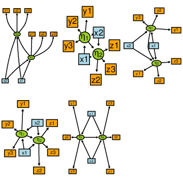
11 Application: Brain serotonin transporter imaging data

We consider 54 observations from (Kalbitzer et al, 2010) with measurements of the serotonin transporter (SERT) in the human brain as measured by Positron Emission Tomography (PET) techniques. The outcome of interest, SERT, was quantified as binding potential of the specific tracer binding ( $\text{BP}_{ND}$ ) in four regions of interest, which a priori were identified as high-binding and reliable measurements of SERT. The serotonergic system has been suggested to have a strong impact on mood and as a potential predictor of the development of seasonal affective disorder (SAD). The aim of the original study was to explore the association between levels of SERT and the interaction between seasonality and a repeat polymorphism in the promoter region of the serotonin transporter gene (5-HTTLPR). This was achieved by linear regression on each regional outcome. However, these data are characterized by high inter-regional correlation, and in the following we will supplement the original analysis with a multivariate analysis taking this aspect into account. It has been demonstrated that SERT levels respond to chronic changes in brain serotonin (5-HT) levels as suggested by studies of the effect of SSRI treatment and in animal studies. It has therefore been suggested that the common regulator of SERT is this underlying 5-HT level (Erritzoe et al, 2010) which, however, cannot be measured directly in vivo. This biological model can be captured by a structural equation model, with a simple measurement model describing the four regions of interest, and a structural model in which exogenous variables affects the SERT measurements indirectly through the intermediate latent variable as shown on Figure 15.

We chose to model the seasonal effect using a harmonic function with a period of one year, described by the amplitude, $A$ , and the translation parameter, $\delta$ (time of peak):

\displaystyle A\cos\left(\frac{2\pi(t-\delta)}{365}\right)=\underbrace{A\cos\left(\frac{2\pi\delta}{365}\right)}_{\beta_{1}}\cos\left(\frac{2\pi t}{365}\right)+\underbrace{A\sin\left(\frac{2\pi\delta}{365}\right)}_{\beta_{2}}\sin\left(\frac{2\pi t}{365}\right),

(95)

where $t$ is the date of the scan. This parameterization approximately embeds a simpler model, where the seasonal effect is described as a linear function of the amount of daylight minutes on the date of the PET scan. However, the harmonic curve adds the flexibility of letting the time of peak be a free parameter which allows a possible delayed seasonal effects on the serotonin transporter to be taken into account. In lava the seasonal effect could be modeled directly (via constrain) as the left-hand-side of (95), thus directly quantifying $A$ and $\delta$ . Here we use the linear parameterization on the right-hand-side using the cosine and sine transformed time variables as predictors. As in the original study, we also adjust for possible main effects of age, gender and the 5-HTTLPR polymorphism (dichotomized as carriers of the (short) s-variation vs. non-carriers (long-long alleles))

> httmod <- lvm(c(cau,th,put,mid) ˜ eta)> regression(httmod) <- eta ˜ f(cos,b1)+f(sin,b2)+age+sex+gene

As described in Section 6, we assessed the model fit via residual plots, score tests and the global $\chi^{2}$ -test, and concluded that the local independence between the midbrain and thalamus region was not plausible. Significantly different age and gender effects on caudate nucleus were also identified in this process and therefore added to the model.

> regression(httmod) <- cau˜sex+age> covariance(httmod) <- th˜midNo additional evidence against the model was identified, thus leading to a final model as illustrated in Figure 16:

> tikz(file="sertsem1.tex",8,8,standAlone=TRUE)> m <- lvm(˜cau+th+put+mid)> regression(m) <- c(cau,mid,th,put)˜eta> latent(m) <- ˜eta; labels(m) <- c(eta="$\\eta$")> regression(m) <- eta˜sex+age+date> nodecolor(m,vars(m)) <- 0> nodecolor(m,endogenous(m),labcol="white") <-+ c("red","blue","green","orange")> plot(m)> dev.off()

Parameter estimates are obtained by maximum likelihood using a Newton-Raphson algorithm:

> lava.options(method="NR",trace=1,tol=1e-12,param="relative")> httmod.fit <- estimate(httmod,data=dasb)

One of the aims of the analysis is to quantify the seasonal effect, therefore we will also estimate the translation and amplitude (unsigned)

\displaystyle\widehat{\delta}=\arctan(\widehat{\beta}_{2}/\widehat{\beta}_{1})365/(2\pi)

(96)

\displaystyle|\widehat{A}|=\sqrt{\widehat{\beta}_{1}^{2}+\widehat{\beta}_{2}^{2}}

(97)

> constrain(httmod.fit,delta˜b1+b2) <- function(x) atan(x[2]/x[1])*365/(2*pi)> constrain(httmod.fit,A˜b1+b2) <- function(x) sqrt(x[1]ˆ2+x[2]ˆ2)> summary(httmod.fit, std=NULL)

||score||ˆ2= 1.171417e-11Latent variables: etaNumber of rows in data= 54-------------------------------------------------- Estimate Std. Error Z value Pr(>|z|)Measurements: cau<-eta 1.0000e+00 th<-eta 9.6834e-01 3.0972e-01 3.1264e+00 1.7693e-03 put<-eta 1.2119e+00 3.5519e-01 3.4120e+00 6.4499e-04 mid<-eta 1.1317e+00 7.5972e-01 1.4896e+00 1.3633e-01Regressions: cau<-age 6.7822e-03 1.9574e-03 3.4648e+00 5.3054e-04 cau<-sex -3.2907e-01 7.4087e-02 -4.4416e+00 8.9284e-06 b1:eta<-cos 1.0722e-01 3.9546e-02 2.7112e+00 6.7043e-03 b2:eta<-sin -3.7658e-02 4.1421e-02 -9.0915e-01 3.6327e-01 eta<-age -2.9471e-03 1.4856e-03 -1.9838e+00 4.7282e-02 eta<-sex -7.8173e-03 4.9608e-02 -1.5758e-01 8.7479e-01 eta<-GnonLL -4.5062e-02 4.7688e-02 -9.4494e-01 3.4469e-01Intercepts: cau 0.0000e+00 th 2.8698e-01 5.9078e-01 4.8577e-01 6.2713e-01 put -4.1726e-01 6.8945e-01 -6.0521e-01 5.4504e-01 mid 2.0487e+00 1.4175e+00 1.4453e+00 1.4838e-01 eta 1.9647e+00 8.7535e-02 2.2445e+01 <1e-16Residual Variances: cau 5.4901e-02 1.2519e-02 4.3855e+00 th 6.9573e-02 1.4911e-02 4.6658e+00 th,mid 9.6725e-02 3.4453e-02 2.8074e+00 4.9940e-03 put 1.0455e-02 9.2801e-03 1.1266e+00 mid 6.9218e-01 1.3472e-01 5.1377e+00 eta 2.0335e-02 9.8548e-03 2.0635e+00Non-linear constraints: Estimate Std. Error Z value Pr(>|z|) 2.5% 97.5%delta -19.6215810 19.5444140 -1.0039483 0.3154035 -57.9279285 18.6848A 0.1136378 0.0426363 2.6652834 0.0076923 0.0300722 0.1972--------------------------------------------------Estimator: gaussian--------------------------------------------------Number of observations = 54 Log-Likelihood = -57.88782 BIC = 223.2812 AIC = 155.7756 log-Likelihood of model = -57.88782 log-Likelihood of saturated model = -46.94523 Chi-squared statistic: Q = 21.88517 , df = 14 , P(Q>q) = 0.08100473--------------------------------------------------

As an alternative to the Wald test we can conduct a LRT to test the significance of the seasonal parameters:

> httmod0 <- httmod; kill(httmod0) <- ˜cos+sin> httmod0.fit <- estimate(httmod0,dd,control=list(start=coef(httmod.fit)))> compare(httmod0.fit,httmod.fit)

Likelihood ratio testdata:chisq = 12.3978, df = 2, p-value = 0.002032sample estimates:log likelihood (model 1) log likelihood (model 2) -64.53133 -58.33241

Thus, we find a highly significant seasonal effect ( $p=0.002$ ). The estimated time of peak and 95% Wald confidence limits can be quantified as

> format(as.Date("2010-1-1")+constraints(httmod.fit)["delta",c(1,5:6)],+ "%d%b")

Estimate 2.5% 97.5% "12Dec" "04Nov" "19Jan"and with an estimate around middle of December this is in reasonable agreement with a suggested peak around winter solstice (about December 21). The parameter estimates of the initial model (Figure 15) yielded very similar seasonal parameter estimates and confidence limits.

Next, we will examine the interaction between season and the 5-HTTLPR polymorphism. This is done via a multigroup analysis and hence we divide the data into two groups defined by the genetic variable

> d1 <- subset(dd, G=="LL")> d2 <- subset(dd, G=="nonLL")A standard multigroup analysis could be conducted where the parameters $\beta_{1}$ and $\beta_{2}$ would be allowed to vary freely in the two groups. However, a more biological plausible model is to fix the translation parameter $\delta$ in the two groups to be the same and let the amplitude $A$ be free. This can be implemented via the left-hand-side of (95) and the constrain-method

> m <- baptize(kill(httmod,˜G+cos+sin))> intercept(m,˜cau+eta) <- list(0,"mu1")> regression(m,cau˜eta) <- 1> regression(m,eta˜Day) <- 0> m2 <- m> intercept(m2,˜eta) <- "mu2"> mycos <- function(x) x[2]+x[3]*cos(2*pi*(x[1]-x[4])/365)> constrain(m,mu˜Day+nu1+A1+delta) <- mycos> constrain(m2,mu2˜Day+nu2+A2+delta) <- mycosHere we explicitly chose caudate nucleus as our reference region by fixing the factor loading to 1 and intercept to 0. The intercept parameters nu1 and nu2 describes the main effect of the genotype. The significance of the interaction can then be examined with a LRT against the first model

> httmod.2 <- estimate(list(m,m2),list(d1,d2))> compare(httmod.2,httmod.fit)

Likelihood ratio testdata:chisq = 4.7267, df = 1, p-value = 0.0297sample estimates:log likelihood (model 1) log likelihood (model 2) -55.52446 -57.88782The estimated amplitude parameters with 95% confidence limits are

> confint(httmod.2)[c("A1","A2"),c(1,3,4)]

Estimate Pr(>|z|) 2.5%A1 0.01672275 0.691577803 -0.06589577A2 0.14670814 0.002547141 0.05142227and the difference in amplitude can be quantified as

> constrain(httmod.2, dA˜A1+A2) <- diff> constraints(httmod.2)["dA",]

Estimate Std. Error Z value Pr(>|z|) 2.5% 97.5%0.129985393 0.061819428 2.102662508 0.035495282 0.008821541 0.251149245with peak time around January 1:

coef(httmod.2)[[1]]["delta",]

Estimate Std. Error Z value Pr(>|z|) 0.24805873 17.55228131 0.01413256 0.98872422Hence we see a statistical significant difference in amplitude between the two genotypes ( $p=0.03$ , 95% confidence limits $[0.01;0.25]$ ), with carriers of the short 5-HTTLPR allele having on average a higher seasonal variation in SERT binding.

To visualize the harmonic curves of the two genotypes we need to predict the parameters mu1 and mu2. This can also be achieved with constraints where we supply the argument idx indicating which non-linear parameter to extract. For a multigroup model we also need to specify which group to extract this parameter from via the argument k. For instance predicting the two means on each day of the year with 95% confidence limits we can write

> mu1 <- constraints(e,k=1,idx="mu",data=data.frame(Day=1:365),level=0.95)> mu2 <- constraints(e,k=2,idx="mu2",data=data.frame(Day=1:365),level=0.95)See Figure 17 for a plot of these two curves.

This study shows that S-allele carriers (nonLL) on average have a much more varying SERT binding level which could suggest a decreased serotonin concentration in the winter in this group. This could be caused by the decreasing amount of daylight in this period in the study country (Denmark) and supplements previous studies showing that S-allele carriers have higher risk of developing SAD. A detailed discussion can be found in the original paper (Kalbitzer et al, 2010).

12 Conclusion

A package lava has been developed which covers the classical covariance structure analysis and which hopefully can serve as a platform for methodological development in the field of structural equation models and related models.

The key features of the package is

1.

Easy interactive specification and visualization of complex models
2.

Simulation routines (for a broad class of models beyond the LLVM)
3.

Extensions to binary and censored data via lava.tobit
4.

Multigroup analyses
5.

MLE with data missing at random
6.

Non-linear parameter constraints and covariate effects
7.

Asymptotically correct standard errors for clustered correlated data

Further, the program is built up around a series of modules (optimizers, estimators, plot hooks, simulations hooks, pre and post estimation hooks) which should ensure that future extensions can be written quite easily. This has been one of the main aims during the development of the lava package.

Additional extensions of the package is currently under preparation including non-linear random effects and MLE for a broader class of the exponential family with estimation based on adaptive quadrature rules. In this process, we are preparing to export loop-intensive parts of the program to C++, which also should give a considerable computational and memory (via call-by-reference) improvement for some of the closed-form likelihood models (e.g. random slope models) and models with large number of variables.

If you use lava please cite this paper and the R software in publications.

13 Acknowledgments

This work was supported by The Danish Agency for Science, Technology and Innovation.

Appendix A Some zero-one matrices

In this section we will define a few matrix-operators in order to define various conditional moments. Let $\bm{B}\in\mathbb{R}^{n\times m}$ be a matrix, and define the indices $\bm{x}=\{x_{1},\ldots,x_{k}\}\in\{1,\ldots,n\}$ , and $\bm{y}=\{y_{1},\ldots,y_{l}\}\in\{1,\ldots,m\}$ . We define $\bm{J}_{n,\bm{x}}=\bm{J}_{\bm{x}}\in\mathbb{R}^{(n-k)\times n}$ as the $n\times n$ identify matrix with rows $\bm{x}$ removed. E.g.

\displaystyle\bm{J}_{6,(3,4)}=\left(\begin{array}[]{cccccc}1&0&0&0&0&0\\ 0&1&0&0&0&0\\ 0&0&0&0&1&0\\ 0&0&0&0&0&1\\ \end{array}\right).

To remove rows $\bm{x}$ from $\bm{B}$ we simply multiply from the left with $\bm{J}_{n,\bm{x}}$ . If we in addition want to remove columns $\bm{y}$ we multiply with the transpose of $\bm{J}_{n,\bm{y}}$ from the right:

\displaystyle\bm{J}_{n,\bm{x}}\bm{B}\bm{J}_{n,\bm{y}}^{\prime}.

(98)

We will use the notation $\bm{J}$ to denote the matrix that removes all latent variables ( $\bm{\eta}$ ) from the vector of all variable, $\bm{U}$ as defined in (8). We denote $\bm{J}_{\bm{Y}}$ the matrix that only keeps endogenous variables ( $\bm{Y}$ ).

We also need an operator that cancels out rows or columns of a matrix/vector. Define the square matrix $\bm{p}_{n,\bm{x}}\in\mathbb{R}^{n\times n}$ as the identity-matrix with diagonal elements at position $\bm{x}$ canceled out:

\displaystyle\bm{p}_{n,\bm{x}}(i,j)=\begin{cases}1,&i=j,\ i\not\in\bm{x},\\ 0,&\text{else}.\end{cases}

(99)

E.g.

\displaystyle\bm{p}_{6,(3,4)}=\left(\begin{array}[]{cccccc}1&0&0&0&0&0\\ 0&1&0&0&0&0\\ 0&0&0&0&0&0\\ 0&0&0&0&0&0\\ 0&0&0&0&1&0\\ 0&0&0&0&0&1\\ \end{array}\right).

To cancel out rows $\bm{x}$ and columns $\bm{y}$ of the matrix $\bm{B}\in\mathbb{R}^{n\times m}$ we calculate

\displaystyle\bm{p}_{n,\bm{x}}\bm{B}\bm{p}_{m,\bm{y}}^{\prime}.

We will use $\bm{p}_{\bm{X}}$ and $\bm{p}_{\complement\bm{X}}$ as the matrix that cancels out the rows corresponding to the index of the exogenous variables ( $\bm{X}$ ) respectively the matrix that cancels out all rows but the ones corresponding to $\bm{X}$ .

Appendix B The Score Function and Information

In this section we will calculate the analytical derivatives of the log-likelihood. In order to obtain these results we will first introduce the notation of some common matrix operations. Let $\bm{A}\in\mathbb{R}^{m\times n}$ , then we define the column-stacking operation:

\displaystyle\operatorname{vec}(\bm{A})=\begin{pmatrix}a_{1}\\ \vdots\\ a_{n}\end{pmatrix},

where $a_{i}$ denotes the $i$ th column of $\bm{A}$ . The unique commutation matrix, $\mathbb{R}^{mn\times mn}$ is defined by

\displaystyle\bm{K}^{(m,n)}\operatorname{vec}(\bm{A})=\operatorname{vec}(\bm{A}^{\prime}).

(100)

Letting $\bm{H}^{(i,j)}$ be the $m\times n$ -matrix with one at position $(i,j)$ and zero elsewhere, then

\displaystyle\bm{K}^{(m,n)}=\sum_{i=1}^{m}\sum_{j=1}^{n}(\bm{H}^{(i,j)}\otimes\bm{H}^{(i,j)}{}^{\prime}),

e.g.

\displaystyle\bm{K}^{(2,3)}=\left(\begin{array}[]{cc:cc:cc}1&0\hfil\lx@intercol\vrule\lx@add@cssclass&0&0\hfil\lx@intercol\vrule\lx@add@cssclass&0&0\\ 0&0\hfil\lx@intercol\vrule\lx@add@cssclass&1&0\hfil\lx@intercol\vrule\lx@add@cssclass&0&0\\ 0&0\hfil\lx@intercol\vrule\lx@add@cssclass&0&0\hfil\lx@intercol\vrule\lx@add@cssclass&1&0\\ \hline\cr 0&1\hfil\lx@intercol\vrule\lx@add@cssclass&0&0\hfil\lx@intercol\vrule\lx@add@cssclass&0&0\\ 0&0\hfil\lx@intercol\vrule\lx@add@cssclass&0&1\hfil\lx@intercol\vrule\lx@add@cssclass&0&0\\ 0&0\hfil\lx@intercol\vrule\lx@add@cssclass&0&0\hfil\lx@intercol\vrule\lx@add@cssclass&0&1\\ \end{array}\right).

It should be noted that product with a commutation matrix can be implemented very efficiently instead of relying on a direct implementation of the above mathematical definition.

Let $\bm{A}\in\mathbb{R}^{m\times n}$ and $\bm{B}\in\mathbb{R}^{p\times q}$ then the Kronecker product is the $mp\times nq$ -matrix:

\displaystyle\bm{A}\otimes\bm{B}=\begin{pmatrix}a_{11}\bm{B}&\cdots&a_{1n}\bm{B}\\ \vdots&&\vdots\\ a_{m1}\bm{B}&\cdots&a_{mn}\bm{B}\\ \end{pmatrix}

We will calculate the derivatives of (20) by means of matrix differential calculus. The Jacobian matrix of a matrix-function $F\colon\mathbb{R}^{n}\to\mathbb{R}^{m\times p}$ is the $mp\times n$ matrix defined by

\displaystyle DF(\bm{\theta})=\frac{\partial\operatorname{vec}F(\bm{\theta})}{\partial\bm{\theta}^{\prime}}.

Letting $\operatorname{d}\!\,$ denote the differential operator (see Magnus and Neudecker (1988)), the first identification rule states that $\operatorname{d}\!\,\operatorname{vec}F(\bm{\theta})=A(\bm{\theta})\operatorname{d}\!\,\bm{\theta}\Rightarrow DF(\bm{\theta})=A(\bm{\theta})$ .

B.0.1 Score function

Using the identities $\operatorname{d}\!\,\log\left|\bm{X}\right|=\tr(\bm{X}^{-1}\operatorname{d}\!\,\bm{X})$ and $\operatorname{d}\!\,\bm{X}^{-1}=-\bm{X}^{-1}(\operatorname{d}\!\,\bm{X})\bm{X}^{-1}$ , and applying the product rule we get

	$\displaystyle\operatorname{d}\!\,\ell(\bm{\theta})$	$\displaystyle=-\frac{n}{2}\tr({\bm{\Omega}}_{\bm{\theta}}^{-1}\operatorname{d}\!\,{\bm{\Omega}}_{\bm{\theta}})-\frac{n}{2}\tr(\operatorname{d}\!\,\{\widehat{\bm{\Sigma}}{\bm{\Omega}}_{\bm{\theta}}^{-1}\})$		(101)
		$\displaystyle=-\frac{n}{2}\tr({\bm{\Omega}}_{\bm{\theta}}^{-1}\operatorname{d}\!\,{\bm{\Omega}}_{\bm{\theta}})+\frac{n}{2}\tr(\widehat{\bm{\Sigma}}{\bm{\Omega}}_{\bm{\theta}}^{-1}[\operatorname{d}\!\,{\bm{\Omega}}_{\bm{\theta}}]{\bm{\Omega}}_{\bm{\theta}}^{-1}),$		(102)

where

$\displaystyle\operatorname{d}\!\,{\bm{\Omega}}_{\bm{\theta}}$	$\displaystyle=\left\{\operatorname{d}\!\,{\bm{G}}_{\bm{\theta}}\right\}{\bm{P}}_{\bm{\theta}}{\bm{G}}_{\bm{\theta}}^{\prime}+{\bm{G}}_{\bm{\theta}}\left\{\operatorname{d}\!\,{\bm{P}}_{\bm{\theta}}{\bm{G}}_{\bm{\theta}}^{\prime}\right\}$	(103)
	$\displaystyle=\left\{\operatorname{d}\!\,{\bm{G}}_{\bm{\theta}}\right\}{\bm{P}}_{\bm{\theta}}{\bm{G}}_{\bm{\theta}}^{\prime}+{\bm{G}}_{\bm{\theta}}\left\{\operatorname{d}\!\,{\bm{P}}_{\bm{\theta}}\right\}{\bm{G}}_{\bm{\theta}}^{\prime}+{\bm{G}}_{\bm{\theta}}{\bm{P}}_{\bm{\theta}}\left\{\operatorname{d}\!\,{\bm{G}}_{\bm{\theta}}\right\}^{\prime}$	(104)
	$\displaystyle=\left\{\operatorname{d}\!\,{\bm{G}}_{\bm{\theta}}\right\}{\bm{P}}_{\bm{\theta}}{\bm{G}}_{\bm{\theta}}^{\prime}+[\left\{\operatorname{d}\!\,{\bm{G}}_{\bm{\theta}}\right\}{\bm{P}}_{\bm{\theta}}{\bm{G}}_{\bm{\theta}}^{\prime}]^{\prime}+{\bm{G}}_{\bm{\theta}}\left\{\operatorname{d}\!\,{\bm{P}}_{\bm{\theta}}\right\}{\bm{G}}_{\bm{\theta}}^{\prime},$	(105)

and

\displaystyle\operatorname{d}\!\,{\bm{G}}_{\bm{\theta}}=\bm{J}(\bm{1}_{m}-{\bm{A}}_{\bm{\theta}})^{-1}\left\{\operatorname{d}\!\,{\bm{A}}_{\bm{\theta}}\right\}(\bm{1}_{m}-{\bm{A}}_{\bm{\theta}})^{-1}.

(106)

Taking $\operatorname{vec}$ ’s it follows that

\displaystyle\operatorname{d}\!\,\operatorname{vec}{\bm{G}}_{\bm{\theta}}=\left[((\bm{1}_{m}-{\bm{A}}_{\bm{\theta}})^{-1})^{\prime}\otimes{\bm{G}}_{\bm{\theta}}\right]\operatorname{d}\!\,\operatorname{vec}{\bm{A}}_{\bm{\theta}}\operatorname{d}\!\,\bm{\theta},

(107)

hence by the first identification rule

\displaystyle\frac{\partial\operatorname{vec}{\bm{G}}_{\bm{\theta}}}{\partial\bm{\theta}^{\prime}}=\left[((\bm{1}_{m}-{\bm{A}}_{\bm{\theta}})^{-1})^{\prime}\otimes{\bm{G}}_{\bm{\theta}}\right]\frac{\partial\operatorname{vec}{\bm{A}}_{\bm{\theta}}}{\partial\bm{\theta}^{\prime}},

(108)

and similarly

\displaystyle\frac{\partial\operatorname{vec}{\bm{\Omega}}_{\bm{\theta}}}{\partial\bm{\theta}^{\prime}}

\displaystyle=(\bm{1}_{k^{2}}+\bm{K}^{(k,k)})\left[{\bm{G}}_{\bm{\theta}}{\bm{P}}_{\bm{\theta}}\otimes\bm{1}_{k}\right]\frac{\partial\operatorname{vec}{\bm{G}}_{\bm{\theta}}}{\partial\bm{\theta}^{\prime}}+\left[{\bm{G}}_{\bm{\theta}}\otimes{\bm{G}}_{\bm{\theta}}\right]\frac{\partial\operatorname{vec}{\bm{P}}_{\bm{\theta}}}{\partial\bm{\theta}^{\prime}},

(109)

and finally (exploiting the symmetry of ${\bm{\Omega}}_{\bm{\theta}}$ and commutative property under the trace operator) we obtain the gradient

\displaystyle\frac{\partial\ell(\bm{\theta})}{\partial\bm{\theta}}=\frac{n}{2}\left(\frac{\partial\operatorname{vec}{\bm{\Omega}}_{\bm{\theta}}}{\partial\bm{\theta}^{\prime}}\right)^{\prime}\operatorname{vec}\left[{\bm{\Omega}}_{\bm{\theta}}^{-1}\widehat{\bm{\Sigma}}{\bm{\Omega}}_{\bm{\theta}}^{-1}\right]-\frac{n}{2}\left(\frac{\partial\operatorname{vec}{\bm{\Omega}}_{\bm{\theta}}}{\partial\bm{\theta}^{\prime}}\right)^{\prime}\operatorname{vec}\left[{\bm{\Omega}}_{\bm{\theta}}^{-1}\right].

(110)

Next we examine the model including a mean structure (20). W.r.t. to the first differential we observe that

\displaystyle\operatorname{d}\!\,\tr\left\{{\bm{T}}_{\bm{\theta}}{\bm{\Omega}}_{\bm{\theta}}^{-1}\right\}

\displaystyle=-\tr\left\{{\bm{T}}_{\bm{\theta}}{\bm{\Omega}}_{\bm{\theta}}^{-1}(\operatorname{d}\!\,{\bm{\Omega}}_{\bm{\theta}}){\bm{\Omega}}_{\bm{\theta}}^{-1}\right\}+\tr\left\{(\operatorname{d}\!\,{\bm{T}}_{\bm{\theta}}){\bm{\Omega}}_{\bm{\theta}}^{-1}\right\}.

(111)

Hence

\displaystyle\begin{split}\frac{\partial\ell(\bm{\theta})}{\partial\bm{\theta}}&=\frac{n}{2}\left(\frac{\partial\operatorname{vec}{\bm{\Omega}}_{\bm{\theta}}}{\partial\bm{\theta}^{\prime}}\right)^{\prime}\operatorname{vec}\left[{\bm{\Omega}}_{\bm{\theta}}^{-1}{\bm{T}}_{\bm{\theta}}{\bm{\Omega}}_{\bm{\theta}}^{-1}\right]-\frac{n}{2}\left(\frac{\partial\operatorname{vec}{\bm{\Omega}}_{\bm{\theta}}}{\partial\bm{\theta}^{\prime}}\right)^{\prime}\operatorname{vec}\left[{\bm{\Omega}}_{\bm{\theta}}^{-1}\right]\\ &\qquad-\frac{n}{2}\left(\frac{\partial\operatorname{vec}{\bm{T}}_{\bm{\theta}}}{\partial\bm{\theta}^{\prime}}\right)^{\prime}\operatorname{vec}\left({\bm{\Omega}}_{\bm{\theta}}^{-1}\right).\end{split}

(112)

Further by the chain-rule

\displaystyle\frac{\partial\operatorname{vec}{\bm{T}}_{\bm{\theta}}}{\partial\bm{\theta}^{\prime}}=\frac{\partial(\widehat{\bm{\mu}}-{\bm{v}}_{\bm{\theta}})}{\partial\bm{\theta}^{\prime}}\frac{\partial\operatorname{vec}{\bm{T}}_{\bm{\theta}}}{\partial(\widehat{\bm{\mu}}-{\bm{\xi}}_{\bm{\theta}})^{\prime}}=-\left[\bm{1}_{k}\otimes(\widehat{\bm{\mu}}-{\bm{\xi}}_{\bm{\theta}})+(\widehat{\bm{\mu}}-{\bm{\xi}}_{\bm{\theta}})\otimes\bm{1}_{k}\right]\frac{\partial{\bm{\xi}}_{\bm{\theta}}}{\partial\bm{\theta}^{\prime}},

(113)

and

\displaystyle\operatorname{d}\!\,{\bm{\xi}}_{\bm{\theta}}=(\operatorname{d}\!\,{\bm{G}}_{\bm{\theta}}){\bm{v}}_{\bm{\theta}}+{\bm{G}}_{\bm{\theta}}(\operatorname{d}\!\,{\bm{v}}_{\bm{\theta}}).

(114)

Taking $\operatorname{vec}$ ( ${\bm{G}}_{\bm{\theta}}{\bm{v}}_{\bm{\theta}}=\bm{1}{\bm{G}}_{\bm{\theta}}{\bm{v}}_{\bm{\theta}}$ ):

\displaystyle\frac{\partial{\bm{\xi}}_{\bm{\theta}}}{\partial\bm{\theta}^{\prime}}=({\bm{v}}_{\bm{\theta}}^{\prime}\otimes\bm{1}_{k})\frac{\partial\operatorname{vec}{\bm{G}}_{\bm{\theta}}}{\partial\bm{\theta}^{\prime}}+{\bm{G}}_{\bm{\theta}}\frac{\partial{\bm{v}}_{\bm{\theta}}}{\partial\bm{\theta}^{\prime}}.

(115)

We have calculated the full score but in some situations it will be useful to evaluate the score in a single point. The contribution of a single observation to the log-likelihood is

\displaystyle\ell(\bm{\theta}\mid\bm{z}_{i})\propto\frac{1}{2}\log\left|{\bm{\Omega}}_{\bm{\theta}}\right|+\frac{1}{2}(\bm{z}_{i}-{\bm{\xi}}_{\bm{\theta}})^{\prime}{\bm{\Omega}}_{\bm{\theta}}^{-1}(\bm{z}_{i}-{\bm{\xi}}_{\bm{\theta}}),

(116)

or as in (20) where we simply exchange ${\bm{T}}_{\bm{\theta}}$ with $\bm{T}_{\bm{z}_{i},\bm{\theta}}=(\bm{z}_{i}-{\bm{\xi}}_{\bm{\theta}})(\bm{z}_{i}-{\bm{\xi}}_{\bm{\theta}})^{\prime}$ , hence the score is as in (112) where (113) is calculated with $\bm{z}_{i}$ instead of $\widehat{\bm{\mu}}$ . Alternatively, letting $\bm{z_{i}}-{\bm{\xi}}_{\bm{\theta}}={\bm{u}}_{\bm{\theta}}={\bm{u}}_{\bm{\theta}}(i)$ :

\displaystyle\begin{split}\operatorname{d}\!\,({\bm{u}}_{\bm{\theta}}^{\prime}{\bm{\Omega}}_{\bm{\theta}}^{-1}{\bm{u}}_{\bm{\theta}})&={\bm{u}}_{\bm{\theta}}^{\prime}\left[(2{\bm{\Omega}}_{\bm{\theta}}^{-1})\operatorname{d}\!\,{\bm{u}}_{\bm{\theta}}+(\operatorname{d}\!\,{\bm{\Omega}}_{\bm{\theta}}^{-1}){\bm{u}}_{\bm{\theta}}\right]\\ &=-{\bm{u}}_{\bm{\theta}}^{\prime}\left[(2{\bm{\Omega}}_{\bm{\theta}}^{-1})\operatorname{d}\!\,{\bm{\xi}}_{\bm{\theta}}+{\bm{\Omega}}_{\bm{\theta}}^{-1}(\operatorname{d}\!\,{\bm{\Omega}}_{\bm{\theta}}){\bm{\Omega}}_{\bm{\theta}}^{-1}{\bm{u}}_{\bm{\theta}}\right],\end{split}

(117)

where we used that for constant symmetric $\bm{A}$ the differential of a quadratic form is

\displaystyle\operatorname{d}\!\,(\bm{u}^{\prime}\bm{A}\bm{u})=2\bm{u}^{\prime}(\bm{A})\operatorname{d}\!\,\bm{u}.

(118)

Hence the contribution to the score function of the $i$ th observation is

\displaystyle\begin{split}\mathcal{S}_{i}(\bm{\theta})&=-\frac{1}{2}\Big\{\operatorname{vec}({\bm{\Omega}}_{\bm{\theta}}^{-1})\frac{\partial\operatorname{vec}{\bm{\Omega}}_{\bm{\theta}}}{\partial\bm{\theta}^{\prime}}-2{\bm{u}}_{\bm{\theta}}^{\prime}{\bm{\Omega}}_{\bm{\theta}}^{-1}\frac{\partial\operatorname{vec}{\bm{\xi}}_{\bm{\theta}}}{\partial\bm{\theta}^{\prime}}\\ &\qquad-({\bm{u}}_{\bm{\theta}}^{\prime}{\bm{\Omega}}_{\bm{\theta}}^{-1}\otimes{\bm{u}}_{\bm{\theta}}^{\prime}{\bm{\Omega}}_{\bm{\theta}}^{-1})\frac{\partial\operatorname{vec}{\bm{\Omega}}_{\bm{\theta}}}{\partial\bm{\theta}^{\prime}}\Big\}\\ &=-\frac{1}{2}\left\{\left(\operatorname{vec}({\bm{\Omega}}_{\bm{\theta}}^{-1})-\operatorname{vec}({\bm{\Omega}}_{\bm{\theta}}^{-1}{\bm{u}}_{\bm{\theta}}{\bm{u}}_{\bm{\theta}}^{\prime}{\bm{\Omega}}_{\bm{\theta}}^{-1})\right)\frac{\partial\operatorname{vec}{\bm{\Omega}}_{\bm{\theta}}}{\partial\bm{\theta}^{\prime}}-2{\bm{u}}_{\bm{\theta}}^{\prime}{\bm{\Omega}}_{\bm{\theta}}^{-1}\frac{\partial\operatorname{vec}{\bm{\xi}}_{\bm{\theta}}}{\partial\bm{\theta}^{\prime}}\right\},\end{split}

(119)

where the score-function evaluated in $\bm{\theta}$ is $\mathcal{S}(\bm{\theta})=\sum_{i=1}^{n}\mathcal{S}_{i}(\bm{\theta})$ .

B.0.2 The Information matrix

The second order partial derivative is given by

\displaystyle\frac{\partial\ell(\bm{\theta})}{\partial\theta_{i}\theta_{j}}=-\frac{1}{2}\frac{\partial}{\partial\theta_{i}}\left[\left\{\operatorname{vec}({\bm{\Omega}}_{\bm{\theta}}^{-1})-\operatorname{vec}({\bm{\Omega}}_{\bm{\theta}}^{-1}{\bm{u}}_{\bm{\theta}}{\bm{u}}_{\bm{\theta}}^{\prime}{\bm{\Omega}}_{\bm{\theta}}^{-1})\right\}\frac{\partial\operatorname{vec}{\bm{\Omega}}_{\bm{\theta}}}{\partial\theta_{j}}-2{\bm{u}}_{\bm{\theta}}^{\prime}{\bm{\Omega}}_{\bm{\theta}}^{-1}\frac{\partial{\bm{\xi}}_{\bm{\theta}}}{\partial\theta_{j}}\right].

(120)

Taking negative expectation with respect to the true parameter $\bm{\theta}_{0}$ we obtain the expected information (Magnus and Neudecker, 1988), which get rid of all second order derivatives

	$\displaystyle\mathcal{I}(\bm{\theta}_{0})$	$\displaystyle=\frac{1}{2}\left(\left.\frac{\partial\operatorname{vec}{\bm{\Omega}}_{\bm{\theta}}}{\partial\bm{\theta}^{\prime}}\right\|_{\bm{\theta}=\bm{\theta}_{0}}\right)^{\prime}(\bm{\Omega}_{\bm{\theta}_{0}}^{-1}\otimes\bm{\Omega}_{\bm{\theta}_{0}}^{-1})\left(\left.\frac{\partial\operatorname{vec}{\bm{\Omega}}_{\bm{\theta}}}{\partial\bm{\theta}^{\prime}}\right\|_{\bm{\theta}=\bm{\theta}_{0}}\right)$		(121)
		$\displaystyle\quad+\left(\left.\frac{\partial{\bm{\xi}}_{\bm{\theta}}}{\partial\bm{\theta}^{\prime}}\right\|_{\bm{\theta}=\bm{\theta}_{0}}\right)^{\prime}\bm{\Omega}_{\bm{\theta}_{0}}^{-1}\left(\left.\frac{\partial{\bm{\xi}}_{\bm{\theta}}}{\partial\bm{\theta}^{\prime}}\right\|_{\bm{\theta}=\bm{\theta}_{0}}\right).$		(122)

We will further derive the observed information in the case where the second derivatives vanishes in the case of the matrix functions ${\bm{A}}_{\bm{\theta}}$ , ${\bm{P}}_{\bm{\theta}}$ and ${\bm{v}}_{\bm{\theta}}$ . Now

\displaystyle\operatorname{d}\!\,^{2}{\bm{G}}_{\bm{\theta}}=\operatorname{d}\!\,\left[\bm{J}(\bm{1}-{\bm{A}}_{\bm{\theta}})^{-1}(\operatorname{d}\!\,{\bm{A}}_{\bm{\theta}})(\bm{1}-{\bm{A}}_{\bm{\theta}})^{-1}\right].

(123)

Hence

\displaystyle\frac{\partial^{2}{\bm{G}}_{\bm{\theta}}}{\partial\theta_{i}\partial\theta_{j}}={\bm{G}}_{\bm{\theta}}\left[\frac{\partial{\bm{A}}_{\bm{\theta}}}{\partial\theta_{i}}(\bm{1}-{\bm{A}}_{\bm{\theta}})^{-1}\frac{\partial{\bm{A}}_{\bm{\theta}}}{\partial\theta_{j}}+\frac{\partial{\bm{A}}_{\bm{\theta}}}{\partial\theta_{j}}(\bm{1}-{\bm{A}}_{\bm{\theta}})^{-1}\frac{\partial{\bm{A}}_{\bm{\theta}}}{\partial\theta_{i}}\right](\bm{1}-{\bm{A}}_{\bm{\theta}})^{-1}.

(124)

Next we will find the derivative of (109). We let $m$ denote the number of variables, $p$ the number of parameters, and $k$ the number of observed variable (e.g. ${\bm{G}}_{\bm{\theta}}\in\mathbb{R}^{k\times m}$ and the number of columns in the derivatives are $p$ ). We have ${\bm{G}}_{\bm{\theta}}{\bm{P}}_{\bm{\theta}}\in\mathbb{R}^{k\times m}$ and using rules for evaluating the differential of Kronecker-product (see Magnus and Neudecker (1988) pp. 184) we obtain

\displaystyle\begin{split}\frac{\partial\operatorname{vec}}{\partial\bm{\theta}^{\prime}}({\bm{G}}_{\bm{\theta}}{\bm{P}}_{\bm{\theta}}\otimes\bm{1}_{k})&=\left(\bm{1}_{m}\otimes\bm{K}^{(k,k)}\otimes\bm{1}_{k}\right)\left(\bm{1}_{km}\otimes\operatorname{vec}\bm{1}_{k}\right)\frac{\partial\operatorname{vec}{\bm{G}}_{\bm{\theta}}{\bm{P}}_{\bm{\theta}}}{\partial\bm{\theta}^{\prime}}\\ &=\left(\bm{1}_{m}\otimes\bm{K}^{(k,k)}\otimes\bm{1}_{k}\right)\left(\bm{1}_{km}\otimes\operatorname{vec}\bm{1}_{k}\right)\times\\ &\qquad\left[({\bm{P}}_{\bm{\theta}}\otimes\bm{1}_{k})\frac{\partial\operatorname{vec}{\bm{G}}_{\bm{\theta}}}{\partial\bm{\theta}^{\prime}}+(\bm{1}_{m}\otimes{\bm{G}}_{\bm{\theta}})\frac{\partial\operatorname{vec}{\bm{P}}_{\bm{\theta}}}{\partial\bm{\theta}^{\prime}}\right].\end{split}

(125)

And

\displaystyle\begin{split}\frac{\partial\operatorname{vec}}{\partial\bm{\theta}}\left[({\bm{G}}_{\bm{\theta}}\otimes{\bm{G}}_{\bm{\theta}})\frac{\partial\operatorname{vec}{\bm{P}}_{\bm{\theta}}}{\partial\bm{\theta}^{\prime}}\right]&=\left[\frac{\partial\operatorname{vec}{\bm{P}}_{\bm{\theta}}}{\partial\bm{\theta}^{\prime}}^{\prime}\otimes\bm{1}_{k^{2}}\right]\frac{\partial\operatorname{vec}{\bm{G}}_{\bm{\theta}}\otimes{\bm{G}}_{\bm{\theta}}}{\partial\bm{\theta}^{\prime}}\\ &=\left[\frac{\partial\operatorname{vec}{\bm{P}}_{\bm{\theta}}}{\partial\bm{\theta}^{\prime}}^{\prime}\otimes\bm{1}_{k^{2}}\right]\left(\bm{1}_{m}\otimes\bm{K}^{(m,k)}\otimes\bm{1}_{k}\right)\times\\ &\qquad\left(\bm{1}_{km}\otimes\operatorname{vec}{\bm{G}}_{\bm{\theta}}+\operatorname{vec}{\bm{G}}_{\bm{\theta}}\otimes\bm{1}_{km}\right)\frac{\partial\operatorname{vec}{\bm{G}}_{\bm{\theta}}}{\partial\bm{\theta}^{\prime}}.\end{split}

(126)

Hence from (125) and (126) and using rules for applying the $\operatorname{vec}$ operator on products of matrices we obtain

\displaystyle\begin{split}\frac{\partial^{2}\operatorname{vec}{\bm{\Omega}}_{\bm{\theta}}}{\partial\bm{\theta}\partial\bm{\theta}^{\prime}}&=\left[\left(\frac{\partial\operatorname{vec}{\bm{G}}_{\bm{\theta}}}{\partial\bm{\theta}^{\prime}}\right)^{\prime}\otimes\left(\bm{1}_{k^{2}}+\bm{K}^{(k,k)}\right)\right]\left(\bm{1}_{m}\otimes\bm{K}^{k+k}\otimes\bm{1}_{k}\right)\left(\bm{1}_{km}\otimes\operatorname{vec}\bm{1}_{k}\right)\times\\ &\qquad\left[({\bm{P}}_{\bm{\theta}}\otimes\bm{1}_{k})\frac{\partial\operatorname{vec}{\bm{G}}_{\bm{\theta}}}{\partial\bm{\theta}^{\prime}}+(\bm{1}_{m}\otimes{\bm{G}}_{\bm{\theta}})\frac{\partial\operatorname{vec}{\bm{P}}_{\bm{\theta}}}{\partial\bm{\theta}^{\prime}}\right]+\\ &\qquad\Big(\bm{1}_{p}\otimes({\bm{G}}_{\bm{\theta}}{\bm{P}}_{\bm{\theta}}\otimes\bm{1}_{k})\Big)\frac{\partial^{2}\operatorname{vec}{\bm{G}}_{\bm{\theta}}}{\partial\bm{\theta}\partial\bm{\theta}^{\prime}}+\\ &\qquad\left(\left(\frac{\partial\operatorname{vec}{\bm{P}}_{\bm{\theta}}}{\partial\bm{\theta}^{\prime}}\right)^{\prime}\otimes\bm{1}_{k^{2}}\right)\left(\bm{1}_{m}\otimes\bm{K}^{(m,k)}\otimes\bm{1}_{k}\right)\times\\ &\qquad\Big(\bm{1}_{km}\otimes\operatorname{vec}{\bm{G}}_{\bm{\theta}}+\operatorname{vec}{\bm{G}}_{\bm{\theta}}\otimes\bm{1}_{km}\Big)\frac{\partial\operatorname{vec}{\bm{G}}_{\bm{\theta}}}{\partial\bm{\theta}^{\prime}},\end{split}

(127)

with the expressions for the derivatives and second derivatives of ${\bm{G}}_{\bm{\theta}}$ given in (108) and (124). Further

\displaystyle\begin{split}\frac{\partial^{2}{\bm{\xi}}_{\bm{\theta}}}{\partial{\bm{\theta}}\partial\bm{\theta}^{\prime}}&=\frac{\partial\operatorname{vec}}{\partial\bm{\theta}^{\prime}}({\bm{v}}_{\bm{\theta}}^{\prime}\otimes\bm{1}_{k})\frac{\partial\operatorname{vec}{\bm{G}}_{\bm{\theta}}}{\partial\bm{\theta}^{\prime}}+\frac{\partial\operatorname{vec}}{\partial\bm{\theta}^{\prime}}{\bm{G}}_{\bm{\theta}}\frac{\partial{\bm{v}}_{\bm{\theta}}}{\partial\bm{\theta}^{\prime}}\\ &=\left(\left(\frac{\partial\operatorname{vec}{\bm{G}}_{\bm{\theta}}}{\partial\bm{\theta}^{\prime}}\right)^{\prime}\otimes\bm{1}_{k}\right)\Big(\bm{1}_{m}\otimes\operatorname{vec}\bm{1}_{k}\Big)\frac{\partial\operatorname{vec}{\bm{v}}_{\bm{\theta}}}{\partial\bm{\theta}^{\prime}}\\ &\qquad+(\bm{1}_{p}\otimes({\bm{v}}_{\bm{\theta}}^{\prime}\otimes\bm{1}_{k}))\frac{\partial^{2}\operatorname{vec}{\bm{G}}_{\bm{\theta}}}{\partial\bm{\theta}\partial\bm{\theta}^{\prime}}\\ &\qquad+\left(\frac{\partial\operatorname{vec}{\bm{G}}_{\bm{\theta}}}{\partial\bm{\theta}^{\prime}}\right)^{\prime}\frac{\partial{\bm{v}}_{\bm{\theta}}}{\partial\bm{\theta}^{\prime}},\end{split}

(128)

and

\displaystyle\frac{\partial\operatorname{vec}}{\partial\bm{\theta}^{\prime}}{\bm{\Omega}}_{\bm{\theta}}^{-1}=-({\bm{\Omega}}_{\bm{\theta}}^{-1}\otimes{\bm{\Omega}}_{\bm{\theta}}^{-1})\frac{\partial\operatorname{vec}{\bm{\Omega}}_{\bm{\theta}}}{\partial\bm{\theta}^{\prime}},

(129)

and

	$\displaystyle\operatorname{d}\!\,\left({\bm{\Omega}}_{\bm{\theta}}^{-1}{\bm{u}}_{\bm{\theta}}{\bm{u}}_{\bm{\theta}}^{\prime}{\bm{\Omega}}_{\bm{\theta}}^{-1}\right)$	$\displaystyle=-{\bm{\Omega}}_{\bm{\theta}}^{-1}(\operatorname{d}\!\,{\bm{\Omega}}_{\bm{\theta}}){\bm{\Omega}}_{\bm{\theta}}^{-1}{\bm{u}}_{\bm{\theta}}{\bm{u}}_{\bm{\theta}}^{\prime}{\bm{\Omega}}_{\bm{\theta}}+{\bm{\Omega}}_{\bm{\theta}}^{-1}(\operatorname{d}\!\,{\bm{u}}_{\bm{\theta}}){\bm{\mu}}_{\bm{\theta}}^{\prime}{\bm{\Omega}}_{\bm{\theta}}^{-1}$		(130)
		$\displaystyle\quad+{\bm{\Omega}}_{\bm{\theta}}^{-1}{\bm{u}}_{\bm{\theta}}(\operatorname{d}\!\,{\bm{u}}_{\bm{\theta}}^{\prime}){\bm{\Omega}}_{\bm{\theta}}^{-1}-{\bm{\Omega}}_{\bm{\theta}}^{-1}{\bm{u}}_{\bm{\theta}}{\bm{u}}_{\bm{\theta}}^{\prime}{\bm{\Omega}}_{\bm{\theta}}(\operatorname{d}\!\,{\bm{\Omega}}_{\bm{\theta}}){\bm{\Omega}}_{\bm{\theta}}^{-1}.$		(131)

By using the identity $\operatorname{vec}(ABC)=(C^{\prime}\otimes A)\operatorname{vec}(B)$ several times we obtain

$\displaystyle\frac{\partial\operatorname{vec}}{\partial\bm{\theta}^{\prime}}{\bm{\Omega}}_{\bm{\theta}}^{-1}{\bm{u}}_{\bm{\theta}}{\bm{u}}_{\bm{\theta}}^{\prime}{\bm{\Omega}}_{\bm{\theta}}^{-1}$	$\displaystyle=-\left([{\bm{\Omega}}_{\bm{\theta}}^{-1}{\bm{u}}_{\bm{\theta}}{\bm{u}}_{\bm{\theta}}^{\prime}{\bm{\Omega}}_{\bm{\theta}}^{-1}]^{\prime}\otimes{\bm{\Omega}}_{\bm{\theta}}^{-1}\right)\frac{\partial\operatorname{vec}{\bm{\Omega}}_{\bm{\theta}}}{\partial\bm{\theta}^{\prime}}$	(132)
	$\displaystyle\quad-\left([{\bm{u}}_{\bm{\theta}}^{\prime}{\bm{\Omega}}_{\bm{\theta}}^{-1}]^{\prime}\otimes{\bm{\Omega}}_{\bm{\theta}}^{-1}\right)\frac{\partial\operatorname{vec}{\bm{\xi}}_{\bm{\theta}}}{\partial\bm{\theta}^{\prime}}$	(133)
	$\displaystyle\quad-\left({\bm{\Omega}}_{\bm{\theta}}^{-1}\otimes[{\bm{\Omega}}_{\bm{\theta}}^{-1}{\bm{u}}_{\bm{\theta}}]\right)\frac{\partial\operatorname{vec}{\bm{\xi}}_{\bm{\theta}}}{\partial\bm{\theta}^{\prime}}$	(134)
	$\displaystyle\quad-\left({\bm{\Omega}}_{\bm{\theta}}^{-1}\otimes[{\bm{\Omega}}_{\bm{\theta}}^{-1}{\bm{u}}_{\bm{\theta}}{\bm{u}}_{\bm{\theta}}^{\prime}{\bm{\Omega}}_{\bm{\theta}}^{-1}]\right)\frac{\partial\operatorname{vec}{\bm{\Omega}}_{\bm{\theta}}}{\partial\bm{\theta}^{\prime}},$	(135)

and the second order derivative of the log-likelihood (120) now follows from applying the product rule with (127), (128), (129) and (132).

References

Andersen (1971) Andersen EB (1971) The asymptotic distribution of conditional likelihood ratio tests. Journal of the American Statistical Association 66(335):pp. 630–633
Angrist (2001) Angrist J (2001) Estimation of limited dependent variable models with dummy endogenous regressors: simple strategies for empirical practice. Journal of Business and Economic Statistics 19:2–16
Bates and Maechler (2009) Bates D, Maechler M (2009) lme4: Linear mixed-effects models using S4 classes. URL http://CRAN.R-project.org/package=lme4, R package version 0.999375-31
Biernacki et al (2005) Biernacki C, Celeux G, Govaert G (2003) Choosing starting values for the EM algorithm for getting the highest likelihood in multivariate Gaussian mixture models. Biometrika 73(1):561-575
Boker et al (2011) Boker S, Neale M, Maes H, Wilde M, Spiegel M, Brick T, Spies J, Estabrook R, Kenny S, Bates T, Mehta P, Fox J (2011) Openmx: An open source extended structural equation modeling framework. Psychometrika 76:306–317, URL http://dx.doi.org/10.1007/s11336-010-9200-6, 10.1007/s11336-010-9200-6
Bollen (1996) Bollen K (1996) An alternative two stage least squares (2sls) estimator for latent variable equations. Psychometrika 61(1):109–121
Bollen (1989) Bollen KA (1989) Structural equations with latent variables. Wiley Series in Probability and Mathematical Statistics: Applied Probability and Statistics, John Wiley & Sons Inc., New York, a Wiley-Interscience Publication
Bollen (2001) Bollen KA (2001) Two-stage least squares and latent variable models: simultaneous estimation and robustness to misspecification. In: Robert Cudeck DS S H C Du Toit (ed) Structural equation modeling, present and future: a festschrift in honor of Karl Jöreskog, Scientific Software International
Bollen et al (2007) Bollen KA, Kirby JB, Curran PJ, Paxton PM, Chen F (2007) Latent variable models under misspecification two-stage least squares (2SLS) and Maximum Likelihood (ML) estimators. Sociol Methods Res 36(1):48–86, DOI 10.1177/0049124107301947
Budtz-Jørgensen et al (2003) Budtz-Jørgensen E, Keiding N, Grandjean P, Weihe P, White RF (2003) Statistical methods for the evaluation of health effects of prenatal mercury exposure. Environmetrics 14:105–120
Caffo and Griswold (2006) Caffo B, Griswold M (2006) A User-Friendly Introduction to Link-Probit-Normal Models. The American Statistician 60(2):139–145
Celeux and Diebolt (1986) Celeux G, Diebolt J (1993) Asymptotic properties of a stochastic EM algorithm for estimating mixing proportions. Comm. Statist. Stochastic Models 9:599-613
REvolution Computing (2009) REvolution Computing (2009) foreach: Foreach looping construct for R. URL http://CRAN.R-project.org/package=foreach, R package version 1.3.0
Diebolt and Ip (1996) Diebolt J, Ip E (1996) Stochastic EM: method and application. W.R. Gilks and S. Richardson and D.J. Speigelhalter (eds), Markov Chain Monte Carlo in Practice:259-273
Dempster et al (1977) Dempster A, Laird N, Rubin D (1993) Maximum Likelihood from Incomplete Data via the EM Algorithm. Journal of Royal Statistical Society 39:1–38
Ditlevsen et al (2005) Ditlevsen S, Christensen U, Lynch J, Damsgaard MT, Keiding N (2005) The mediation proportion: A structural equation approach for estimating the proportion of exposure effect on outcome explained by an intermediate variable. Epidemiology 16(1):114–120, DOI 10.1097/01.ede.0000147107.76079.07
Erritzoe et al (2010) Erritzoe D, Holst KK, Frokjaer VG, Licht CL, Kalbitzer J, Nielsen FA, Svarer C, Madsen J, Knudsen GM (2010) A nonlinear relationship between cerebral serotonin transporter and 5-HT2A receptor binding: An in vivo molecular imaging study in humans. J Neurosci 30(9):3391–3397, DOI 10.1523/JNEUROSCI.2852-09.2010, http://www.jneurosci.org/cgi/reprint/30/9/3391.pdf
Fox (2006) Fox J (2006) Teacher’s corner: Structural equation modeling with the sem package in r. Structural Equation Modeling: A Multidisciplinary Journal 13(3):465–585, DOI 10.1207/s15328007sem1303\_7
Fox (2009) Fox J (2009) sem: Structural Equation Models. URL http://CRAN.R-project.org/package=sem, R package version 0.9-16
Gansner and North (1999) Gansner ER, North SC (1999) An open graph visualization system and its applications to software engineering. Software - Practice and Experience 30:1203–1233
Gentleman et al (2009) Gentleman R, Whalen E, Huber W, Falcon S (2009) graph: graph: A package to handle graph data structures. R package version 1.20.0
Gentleman et al (2004) Gentleman RC, Carey VJ, Bates DM, et al (2004) Bioconductor: Open software development for computational biology and bioinformatics. Genome Biology 5:R80, URL http://genomebiology.com/2004/5/10/R80
Gentry et al (2009) Gentry J, Long L, Gentleman R, Falcon S, Hahne F, Sarkar D (2009) Rgraphviz: Provides plotting capabilities for R graph objects. R package version 1.20.3
Genz et al (2009) Genz A, Bretz F, Miwa T, Mi X, Leisch F, Scheipl F, Hothorn T (2009) mvtnorm: Multivariate Normal and t Distributions. URL http://CRAN.R-project.org/package=mvtnorm, R package version 0.9-4
Gilbert (2009) Gilbert P (2009) numDeriv: Accurate Numerical Derivatives. URL http://www.bank-banque-canada.ca/pgilbert, R package version 2006.4-1
Greene (2002) Greene WH (2002) Econometric Analysis, 5th edn. Prentice Hall
Holm (1979) Holm S (1979) A Simple Sequentially Rejective Multiple Test Procedure. Scandinavian Journal of Statistics 6(2):65–70, DOI 10.2307/4615733
Holst (2011) Holst KK (2011) lava.tobit: Latent variable models with censored and binary outcomes. URL http://lava.r-forge.r-project.org/, R package version 0.4-3
Holst (2012) Holst KK (2012) gof: Model-diagnostics based on cumulative residuals. URL http://CRAN.R-project.org/package=gof, R package version 0.8-1
Horvitz and Thompson (1952) Horvitz DG, Thompson DJ (1952) A generalization of sampling without replacement from a finite universe. Journal of the American Statistical Association 47(260):663–685
Hotelling (1953) Hotelling H (1953) New light on the correlation coefficient and its transforms. J Roy Statist Soc Ser B 15:193–225; discussion, 225–232
Jöreskog (1970) Jöreskog K (1970) A general method for analysis of covariance structures. Biometrika 57:239–251
Kalbitzer et al (2010) Kalbitzer J, Erritzoe D, Holst KK, Nielsen F, Marner L, Lehel S, Arentzen T, Jernigan TL, Knudsen GM (2010) Seasonal changes in brain serotonin transporter binding in short serotonin transporter linked polymorphic region-allele carriers but not in long-allele homozygotes. Biological Psychiatry 67:1033–1039, DOI 10.1016/j.biopsych.2009.11.027
Kenward and Molenberghs (1998) Kenward MG, Molenberghs G (1998) Likelihood based frequentist inference when data are missing at random. Statist Sci 13(3):236–247, DOI 10.1214/ss/1028905886
Laird and Ware (1982) Laird NM, Ware JH (1982) Random-effects models for longitudinal data. Biometrics 38:963–974
Lehmann and Romano (2005) Lehmann EL, Romano JP (2005) Testing statistical hypotheses, 3rd edn. Springer Texts in Statistics, Springer, New York
Liang and Zeger (1986) Liang KY, Zeger S (1986) Longitudinal data analysis using generalized linear models. Biometrika 73(1):13–22
Little and Rubin (2002) Little RJA, Rubin DB (2002) Statistical analysis with missing data, 2nd edn. Wiley Series in Probability and Statistics, Wiley-Interscience [John Wiley & Sons], Hoboken, NJ
Magnus and Neudecker (1988) Magnus JR, Neudecker H (1988) Matrix differential calculus with applications in statistics and econometrics. Wiley Series in Probability and Mathematical Statistics: Applied Probability and Statistics, John Wiley & Sons Ltd., Chichester
McArdle and McDonald (1984) McArdle JJ, McDonald RP (1984) Some algebraic properties of the reticular action model for moment structures. The British journal of mathematical and statistical psychology 37 (2):234–251
Muthén and Muthén (2007) Muthén LK, Muthén BO (2007) Mplus User’s Guide (Version 5), 5th edn. Los Angeles, CA: Muthén & Muthén
Paik (1988) Paik M (1988) Repeated measurement analysis for nonnormal data in small samples. Communications in Statistics - Simulation and Computation 17:1155–1171
Pinheiro and Bates (2000) Pinheiro JC, Bates DM (2000) Mixed-Effects Models in S and S-PLUS. Springer
Pinheiro and Chao (2006) Pinheiro JC, Chao EC (2006) Efficient laplacian and adaptive gaussian quadrature algorithms for multilevel generalized linear mixed models. Journal of Computational and Graphical Statistics 15(1):58–81
R Development Core Team (2010) R Development Core Team (2010) R: A Language and Environment for Statistical Computing. R Foundation for Statistical Computing, Vienna, Austria, URL http://www.R-project.org/, ISBN 3-900051-07-0
Rabe-Hesketh et al (2004) Rabe-Hesketh S, Skrondal A, Pickles A (2004) Generalized multilevel structural equation modeling. Psychometrika 69:167–190, DOI 10.1007/BF02295939
Raftery (1993) Raftery A (1993) Bayesian model selection in structural equation models. In: Bollen K, Long J (eds) Testing Structural Equation Models, Sage, Newbury Park CA, pp 163–180
Rotnitzky and Robins (1995) Rotnitzky A, Robins JM (1995) Semiparametric regression estimation in the presence of dependent censoring. Biometrika 82(4):805–820
Sanchez et al (2005) Sanchez BN, Budtz-Jørgensen E, Ryan LM, Hu H (2005) Structural equation models: A review with applications to environmental epidemiology. J Am Stat Assoc 100:1443–1455
Sharpsteen and Bracken (2010) Sharpsteen C, Bracken C (2010) tikzDevice: A Device for R Graphics Output in PGF/TikZ Format. URL http://R-Forge.R-project.org/projects/tikzdevice/, R package version 0.5.2/r34
Steiger (2001) Steiger JH (2001) Driving fast in reverse. Journal of the American Statistical Association 96(453):331–338, DOI 10.1198/016214501750332893
Therneau and original R port by Thomas Lumley (2009) Therneau T, original R port by Thomas Lumley (2009) survival: Survival analysis, including penalised likelihood. URL http://CRAN.R-project.org/package=survival, R package version 2.35-8
White (1982) White H (1982) Maximum likelihood estimation of misspecified models. Econometrica 50(1):1–26
Williams (2000) Williams RL (2000) A note on robust variance estimation for cluster-correlated data. Biometrics 56(2):645–646, DOI 10.1111/j.0006-341X.2000.00645.x
Yan and Fine (2004) Yan J, Fine J (2004) Estimating equations for association structures. Stat Med 23:859–874, DOI 10.1002/sim.1650