SFB/CPP-12-39 TTP12-20 Moments of heavy quark correlators with two masses: exact mass dependence to three loops

Jonathan Grigo Jens Hoff Peter Marquard Matthias Steinhauser Affiliation: Institut für Theoretische Teilchenphysik, Karlsruhe Institute of Technology (KIT) Affiliation: 76128 Karlsruhe, Germany

Abstract

We compute moments of non-diagonal correlators with two massive quarks. Results are obtained where no restriction on the ratio of the masses is assumed. Both analytical and numerical methods are applied in order to evaluate the two-scale master integrals at three loops. We provide explicit results for the latter which are useful for other calculations. As a by-product we obtain results for the electroweak $\rho$ parameter up to three loops which can be applied to a fourth generation of quarks with arbitrary masses.

PACS numbers: 12.38.Bx, 14.65.Dw, 14.65.Fy

1 QCD corrections to current correlators

In recent years many multi-loop results to current correlators became available. In the massless approximation the state-of-the art are four-loop integrals which have been applied to $\tau$ and $Z$ -boson decays in order to extract $\alpha_{s}$ [1, 2]. On the other hand, in the limit of small external momentum the so-called moments have been obtained also up to four-loop order [3, 4, 5, 6, 7, 8, 9, 10, 11] and both $\alpha_{s}$ and the charm and bottom quark masses could be extracted by comparing to experimental data or lattice simulations [12, 13, 14, 15, 16]. The currents involved in these calculations only couple to one quark flavour.

As far as the non-diagonal correlators, where the external currents couple to two quark flavours with different masses, are concerned results for the moments up to three loops are known for the limit where one mass is zero [17, 18, 19, 20, 21, 22]. At four-loop order the vector and axial-vector correlators have only been computed for vanishing external momentum (see Ref. [23, 24]) in order to obtain four-loop corrections to the electroweak $\rho$ parameter in the Standard Model [25, 23, 24].

It has been argued in Ref. [26] that it would be desirable to have at hand moments of the heavy-light currents also for general values of the two quark masses. The reason to not only consider physical mass values of the involved quarks is related to lattice simulations where often a variety of different masses are considered in order to be able to extrapolate to the mass values of physical interest. In Ref. [22] this task has been solved with the help of expansions around the equal-mass case and around the limit where one mass is much smaller than the other. In this paper we present exact results up to three loops and thus improve the findings of [22].

We adopt the notation from Ref. [22]. Let us nevertheless present the relevant formulas in order to have a self-contained presentation of the results.

The momentum-space correlator formed by a vector ( $v$ ), axial-vector ( $a$ ), scalar ( $s$ ) or pseudo-scalar ( $p$ ) current is given by

	$\displaystyle\left(-q^{2}g_{\mu\nu}+q_{\mu}q_{\nu}\right)\,\Pi^{\delta}(q^{2})+q_{\mu}q_{\nu}\,\Pi^{\delta}_{L}(q^{2})$	$\displaystyle=$	$\displaystyle i\int{\rm d}x\,e^{iqx}\langle 0\|Tj^{\delta}_{\mu}(x)j^{\delta\dagger}_{\nu}(0)\|0\rangle\,,$
	$\displaystyle q^{2}\,\Pi^{\delta}(q^{2})$	$\displaystyle=$	$\displaystyle i\int{\rm d}x\,e^{iqx}\langle 0\|Tj^{\delta}(x)j^{\delta\dagger}(0)\|0\rangle\,,$		(1)

with

\displaystyle j_{\mu}^{v}=\bar{\psi}_{1}\gamma_{\mu}\psi_{2}\,,\quad j_{\mu}^{a}=\bar{\psi}_{1}\gamma_{\mu}\gamma^{5}\psi_{2}\,,\quad j^{s}=\bar{\psi}_{1}\psi_{2}\,,\quad j^{p}=\bar{\psi}_{1}i\gamma^{5}\psi_{2}\,.

(2)

In our calculations we are allowed to use anti-commuting $\gamma_{5}$ since for $\psi_{1}\not=\psi_{2}$ only non-singlet diagrams contribute.

We work in $n_{f}$ -flavour QCD with two massive and $n_{f}-2$ massless quarks. In our final results we adopt the $\overline{\rm MS}$ renormalization scheme both for the parameters (strong coupling constant $\alpha_{s}$ and the quark masses $m_{1}$ and $m_{2}$ ) and the overall renormalization of the correlator which in the following is indicated by a bar.

In the limit $q^{2}\to 0$ the quantity $\bar{\Pi}^{\delta}(q^{2})$ (and analogously $\bar{\Pi}_{L}^{\delta}(q^{2})$ ) can be cast in the form

\displaystyle\bar{\Pi}^{\delta}(q^{2})

\displaystyle=

\displaystyle\frac{3}{16\pi^{2}}\sum_{n\geq-1}\bar{C}^{\delta}_{n}(x)z^{n}\,,

(3)

where the dimensionless variables¹¹ 1 In the following we do not write $m_{1}^{(n_{f})}(\mu)$ and $m_{2}^{(n_{f})}(\mu)$ but suppress the dependence on the renormalization scale $\mu$ and the number of flavours $n_{f}$ .

\displaystyle z=\frac{q^{2}}{m_{1}^{2}}\,,\qquad\mbox{and}\qquad x=\frac{m_{2}}{m_{1}}\,,

(4)

have been introduced. Note that we assume $0\leq x\leq 1$ . Results for $m_{2}>m_{1}$ are easily obtained by interchanging $m_{1}$ and $m_{2}$ . We refer to the coefficients $\bar{C}^{\delta}_{n}(x)$ also as moments. Their perturbative expansion can be written as

\displaystyle\bar{C}^{\delta}_{n}=\bar{C}^{(0),\delta}_{n}+\frac{\alpha_{s}}{\pi}\bar{C}^{(1),\delta}_{n}+\left(\frac{\alpha_{s}}{\pi}\right)^{2}\bar{C}^{(2),\delta}_{n}+\ldots\,,

(5)

where the arguments $x$ and $\mu$ (renormalization scale) are suppressed. Note that we have the symmetry relations $\bar{C}^{s}_{n}(x)=\bar{C}^{p}_{n}(-x)$ and $\bar{C}^{v}_{n}(x)=\bar{C}^{a}_{n}(-x)$ (see, e.g., Ref. [27]) which we use to cross check our results. A further check is provided by computing the moments of the longitudinal contribution $\Pi_{L}^{v,a}(q^{2})$ and compare the result of the moments of $\Pi^{s,p}(q^{2})$ with the help of the relations

	$\displaystyle\bar{C}_{L,n}^{v}$	$\displaystyle=$	$\displaystyle(1-x)^{2}\bar{C}_{n+1}^{s}\,,$
	$\displaystyle\bar{C}_{L,n}^{a}$	$\displaystyle=$	$\displaystyle(1+x)^{2}\bar{C}_{n+1}^{p}\,.$		(6)

For completeness, let us mention that the QED-like normalization of the polarization function with $\Pi^{\delta}(0)=0$ can be obtained from $\bar{\Pi}^{\delta}(q^{2})$ with the help of

\displaystyle\Pi^{\delta}(q^{2})

\displaystyle=

\displaystyle\bar{\Pi}^{\delta}(q^{2})-\frac{3}{16\pi^{2}}\left(\bar{C}^{\delta}_{0}+\frac{\bar{C}^{\delta}_{-1}}{z}\right)\,.

(7)

Sample Feynman diagrams occurring at one-, two- and three-loop order are shown in Fig. 1.

Refer to caption — Figure 1: Sample diagrams contributing to $\Pi^{\delta}$ at one, two and three loops. The thick (upper) and thin (lower) lines correspond to quarks with mass $m_{1}$ and $m_{2}$ , respectively, and the curly lines represent gluons.

2 Master integrals for non-diagonal correlators

For the evaluation of the Feynman diagrams a well-tested chain of programs has been used which works hand-in-hand in order to avoid error-prone manual interactions. Since the reduction to master integrals is nowadays pretty standard we restrict ourselves to a brief description up to this step. The Feynman diagrams are generated with QGRAF [28] and the various diagram topologies are identified and transformed to FORM [29, 30] notation with the help of q2e and exp [31, 32]. In a next step appropriate projectors are applied, the expansion in the external momentum is performed and traces are taken. Afterwards the scalar integrals are mapped to functions which are then passed to FIRE [33] where the reduction to master integrals is performed.

The master integrals which are needed for our calculation are shown in Figs. 2 and 3. At one- and two-loop order there are one and three master integrals, respectively, while at three-loop order the reduction leads to three single-scale (c.f. Fig. 2) and 16 two-scale master (c.f. Fig. 3) integrals. All one- and two-loop integrals and the single-scale three-loop integrals in Fig. 2 are available in the literature (see, e.g., Ref. [34, 35]). For the three-loop integrals in Fig. 3 only partial results exist. In this work these results are checked by independent calculations and results for all integrals are presented. Since the problem at hand is symmetric under the exchange of $m_{1}$ and $m_{2}$ most master integrals come in two variants which are marked by the subscripts “a” and “b”.

2.1 Differential equation method

Most of the master integrals can be calculated with the method of differential equations (see, e.g., Refs. [36, 37, 38, 39, 40, 41]). In the following we exemplify the method for the two-loop master integral $J^{(2)}_{1}$ of Fig. 3 which is given by

\displaystyle J_{1}^{(2)}(x)

\displaystyle=\left(\frac{\mu^{2}}{m_{1}^{2}}\right)^{4-d}m_{1}^{2}\int\mathrm{d}^{d}k_{1}\mathrm{d}^{d}k_{2}\frac{1}{(1-k_{1}^{2})(x^{2}-k_{2}^{2})\left[-(k_{1}-k_{2})^{2}\right]}\,,

(8)

where $d=4-2\epsilon$ is the space-time dimension. The differential equations are derived by taking the derivative with respect to $x$ and reducing the resulting integrals to master integrals. This leads to

\displaystyle\frac{\mathrm{d}}{\mathrm{d}x}J_{1}^{(2)}(x)

\displaystyle=-2x\frac{d-3}{1-x^{2}}J_{1}^{(2)}(x)-\frac{d-2}{x(1-x^{2})}K^{(1)}(1)K^{(1)}(x)\,,

(9)

where $K^{(1)}(x)$ denotes the one-loop integral in Fig. 2 with mass $xm_{1}$ which is given by

K^{(1)}(x)={\cal N}\frac{4}{(d-4)(d-2)}\left(xm_{1}\right)^{2}\,,

(10)

with the normalization

\displaystyle\mathcal{N}

\displaystyle=\left(\frac{\mu^{2}}{m_{1}^{2}}\right)^{\epsilon}i\pi^{d/2}\Gamma(3-d/2)\,.

(11)

To solve the differential equation it is necessary to know the initial condition at either $x=0$ or $x=1$ , which corresponds to the single-scale integrals $K^{(2)}_{1}$ and $K^{(2)}_{2}$ shown in Fig. 2. In this simple example it is possible to solve the differential equation without expanding in $\epsilon$ with the result

\begin{split}J^{(2)}_{1}(x)=&{\cal N}^{2}\,m_{1}^{2}\,\Bigg[\frac{2(1-x^{2})^{1-2\epsilon}\Gamma(-\epsilon)\Gamma(-2+2\epsilon)}{\Gamma(1+\epsilon)}\\ &-\frac{x^{2-2\epsilon}(1-x^{2})^{1-2\epsilon}}{(-1+\epsilon)^{2}\epsilon^{2}}\ _{2}F_{1}\left(2-2\epsilon,1-\epsilon,2-\epsilon,x^{2}\right)\Bigg]\,.\end{split}

(12)

This result agrees with the one given in Ref. [34]. In general it is not possible to obtain a closed solution as in Eq. (12). In those cases one has to expand the original differential equation in $\epsilon$ and thus obtains simpler differential equations for the corresponding coefficients. In our example one gets from Eq. (9) for the first three coefficients

$\displaystyle\frac{\mathrm{d}}{\mathrm{d}x}J^{(2)}_{1,-2}(x)$	$\displaystyle=\frac{2x}{x^{2}-1}J^{(2)}_{1,-2}(x)+\frac{2x}{x^{2}-1}\,,$
$\displaystyle\frac{\mathrm{d}}{\mathrm{d}x}J^{(2)}_{1,-1}(x)$	$\displaystyle=\frac{2x}{x^{2}-1}J^{(2)}_{1,-1}(x)-\frac{4x}{x^{2}-1}J^{(2)}_{1,-2}(x)+\frac{2x(1-2\log x)}{x^{2}-1}\,,$
$\displaystyle\frac{\mathrm{d}}{\mathrm{d}x}J^{(2)}_{1,0}(x)$	$\displaystyle=\frac{2x}{x^{2}-1}J^{(2)}_{1,0}(x)-\frac{4x}{x^{2}-1}J^{(2)}_{1,-1}(x)+\frac{2x(1-2\log x+2\log^{2}x)}{x^{2}-1}\,,$	(13)

where the $J^{(2)}_{1,n}(x)$ denotes the coefficient of the $n^{\rm th}$ order in the expansion in $\epsilon$ . One observes that the structure of the homogeneous part remains the same whereas the inhomogeneous contribution becomes successively more complicated. While solving the differential equations it is advantageous to use Harmonic Polylogarithms (HPLs) [42], which form a special class of functions suitable for these kind of problems. It is particularly convenient to use the implementation in Mathematica from Ref. [43, 44] which allows the application of the method of the variation of constants in order to solve the differential equation in Eq. (13). For our example²² 2 Eq. (13) can be expressed in terms of HPLs with the help of $\textrm{H}_{0}(x)=\log x$ and $\textrm{H}_{0,0}(x)=(\log x)^{2}/2$ . at hand the result looks as follows

\begin{split}J_{1}^{(2)}(x)&=\mathcal{N}^{2}m_{1}^{2}\Bigg[\frac{1}{\epsilon^{2}}\left(-\frac{1}{2}\left(x^{2}+1\right)\right)+\frac{1}{\epsilon}\left(-\frac{3}{2}\left(1+x^{2}\right)+2x^{2}\textrm{H}_{0}(x)\right)\\[5.0pt] &\quad+\frac{\pi^{2}\left(x^{2}-1\right)-21\left(1+x^{2}\right)}{6}+6x^{2}\textrm{H}_{0}(x)-4x^{2}\textrm{H}_{0,0}(x)\\ &\quad-2\left(1-x^{2}\right)\left(\textrm{H}_{1,0}(x)-\textrm{H}_{-1,0}(x)\right)+\mathcal{O}(\epsilon)\Bigg]\,,\end{split}

(14)

which can also be obtained by expanding Eq. (12) and agrees with Ref. [34].

2.2 $J^{(3)}_{5a}$ , $J^{(3)}_{5b}$ , $J^{(3)}_{6a}$ and $J^{(3)}_{6b}$

Some of the three-loop master integrals with two masses ( $J^{(3)}_{5a}$ , $J^{(3)}_{5b}$ , $J^{(3)}_{6a}$ , $J^{(3)}_{6b}$ ) are products of one- and two-loop integrals and can therefore easily be calculated with the result

\begin{split}&J^{(3)}_{5a}(x)=\left[K^{(1)}(1)\right]^{2}K^{(1)}(x)\,,\\ &J^{(3)}_{5b}(x)=K^{(1)}(1)\left[K^{(1)}(x)\right]^{2}\,,\\ &J^{(3)}_{6a}(x)=J^{(2)}_{1}(x)K^{(1)}(1)\,,\\ &J^{(3)}_{6b}(x)=J^{(2)}_{1}(x)K^{(1)}(x)\,,\end{split}

(15)

where $K^{(1)}(x)$ and $J^{(2)}_{1}(x)$ are given in Eqs. (10) and (14), respectively.

2.3 $J^{(3)}_{1}$ , $J^{(3)}_{2}$ , $J^{(3)}_{3}$ , $J^{(3)}_{4}$ , $J^{(3)}_{7a}$ and $J^{(3)}_{7b}$

The method of differential equations described above can immediately be applied to the the three-loop integrals $J^{(3)}_{1}$ , $J^{(3)}_{2}$ , $J^{(3)}_{3}$ , $J^{(3)}_{4}$ , $J^{(3)}_{7a}$ and $J^{(3)}_{7b}$ . $J^{(3)}_{1}$ and $J^{(3)}_{2}$ obey a system of coupled differential equations, as do $J^{(3)}_{3}$ and $J^{(3)}_{4}$ . The integrals $J^{(3)}_{7a}$ and $J^{(3)}_{7b}$ which are symmetric under interchange of $m_{1}$ and $m_{2}$ can be obtained by solving a single differential equation. Solving the differential equations leads to analytical results in terms of HPLs. The integrals needed as initial conditions are shown in Fig. 2. The result for $J^{(3)}_{1}$ is given in Ref. [41]. In this reference also the result for an integral related to $J^{(3)}_{2}$ by integration-by-parts identities is listed. We find agreement including terms of order $\epsilon$ .

To our knowledge the results for $J^{(3)}_{3}$ , $J^{(3)}_{4}$ , $J^{(3)}_{7a}$ and $J^{(3)}_{7b}$ are new. They read

$\displaystyle J_{3}^{(3)}(x)=$	$\displaystyle\mathcal{N}^{3}m_{1}^{4}\Bigg[\frac{x^{2}}{3\epsilon^{3}}+\frac{1}{\epsilon^{2}}\left(\frac{1}{12}\left(-1+16x^{2}-x^{4}\right)-x^{2}\textrm{H}_{0}(x)\right)$
	$\displaystyle+\frac{1}{\epsilon}\left(-\frac{5}{24}\left(3-16x^{2}+3x^{4}\right)+\frac{1}{2}x^{2}\left(-8+x^{2}\right)\textrm{H}_{0}(x)+2x^{2}\textrm{H}_{0,0}(x)\right)$
	$\displaystyle+\frac{1}{48}\left(-145\left(1+x^{4}\right)+4\pi^{2}\left(-1+x^{4}\right)+8x^{2}\left(35+4\zeta_{3}\right)\right)$
	$\displaystyle+\frac{1}{12}x^{2}\left(-4\left(30+\pi^{2}\right)+45x^{2}\right)\textrm{H}_{0}(x)-x^{2}\left(-8+x^{2}\right)\textrm{H}_{0,0}(x)-4x^{2}\textrm{H}_{0,0,0}(x)$
	$\displaystyle-\left(1-x^{4}\right)\left(\textrm{H}_{1,0}(x)-\textrm{H}_{-1,0}(x)\right)-4x^{2}\left(\textrm{H}_{2,0}(x)-\textrm{H}_{-2,0}(x)\right)+\mathcal{O}(\epsilon)\Bigg]\,,$	(16)
$\displaystyle J_{4}^{(3)}(x)$	$\displaystyle=\mathcal{N}^{3}m_{1}^{6}\Bigg[\frac{x^{2}}{3\epsilon^{3}}+\frac{1}{\epsilon^{2}}\left(\frac{1}{36}\left(-2+45x^{2}-6x^{4}+x^{6}\right)-x^{2}\textrm{H}_{0}(x)\right)$
	$\displaystyle\quad+\frac{1}{\epsilon}\Bigg(\frac{1}{24}\left(-10+69x^{2}-26x^{4}+5x^{6}\right)$
	$\displaystyle\qquad+x^{2}\left(-4+x^{2}-\frac{x^{4}}{6}\right)\textrm{H}_{0}(x)+2x^{2}\textrm{H}_{0,0}(x)\Bigg)$
	$\displaystyle\quad+\frac{1}{72}\left(-145-4\pi^{2}\right)+\frac{1}{48}\left(203-4\pi^{2}+32\zeta_{3}\right)x^{2}+\left(-\frac{37}{8}+\frac{\pi^{2}}{6}\right)x^{4}$
	$\displaystyle\quad+\frac{1}{144}\left(145-4\pi^{2}\right)x^{6}-\frac{1}{12}x^{2}\left(124+4\pi^{2}-82x^{2}+15x^{4}\right)\textrm{H}_{0}(x)$
	$\displaystyle\quad+\frac{1}{3}x^{2}\left(24-6x^{2}+x^{4}\right)\textrm{H}_{0,0}(x)-4x^{2}\textrm{H}_{0,0,0}(x)-4x^{2}\left(\textrm{H}_{2,0}(x)-\textrm{H}_{-2,0}(x)\right)$
	$\displaystyle\quad-\frac{1}{3}\left(2+3x^{2}-6x^{4}+x^{6}\right)\left(\textrm{H}_{1,0}(x)-\textrm{H}_{-1,0}(x)\right)+\mathcal{O}(\epsilon)\Bigg]\,,$	(17)
$\displaystyle J_{7a}^{(3)}(x)=$	$\displaystyle\mathcal{N}^{3}m_{1}^{2}\Bigg[\frac{1}{\epsilon^{3}}\left(\frac{-1-x^{2}}{3}\right)+\frac{1}{\epsilon^{2}}\left(-2-\frac{5x^{2}}{3}+2x^{2}\textrm{H}_{0}(x)\right)$
	$\displaystyle+\frac{1}{\epsilon}\left(\frac{1}{3}\left(-25-17x^{2}+\pi^{2}\left(-1+x^{2}\right)\right)+10x^{2}\textrm{H}_{0}(x)\right.$
	$\displaystyle\quad\quad\left.-4x^{2}\textrm{H}_{0,0}(x)-4\left(1-x^{2}\right)\left(\textrm{H}_{1,0}(x)-\textrm{H}_{-1,0}(x)\right)\vphantom{\frac{}{}}\right)$
	$\displaystyle+\frac{1}{3}\left(-90+5\pi^{2}\left(-1+x^{2}\right)+22\zeta_{3}-7x^{2}\left(7+2\zeta_{3}\right)\right)+34x^{2}\textrm{H}_{0}(x)$
	$\displaystyle-20x^{2}\textrm{H}_{0,0}(x)+8x^{2}\textrm{H}_{0,0,0}(x)+\frac{\pi^{2}\left(1-4x^{2}+3x^{4}\right)}{3x^{2}}\left(\textrm{H}_{1}(x)-\textrm{H}_{-1}(x)\right)$
	$\displaystyle-20\left(1-x^{2}\right)\left(\textrm{H}_{1,0}(x)-\textrm{H}_{-1,0}(x)\right)+8\left(1-x^{2}\right)\left(\textrm{H}_{1,0,0}(x)-\textrm{H}_{-1,0,0}(x)\right)$
	$\displaystyle+4\left(-4+\frac{1}{x^{2}}+3x^{2}\right)\left(\textrm{H}_{1,1,0}(x)+\textrm{H}_{-1,-1,0}(x)\right)$
	$\displaystyle+\left(16-\frac{4}{x^{2}}-12x^{2}\right)\left(\textrm{H}_{1,-1,0}(x)+\textrm{H}_{-1,1,0}(x)\right)+\mathcal{O}(\epsilon)\Bigg]\,.$	(18)

$J^{(3)}_{7b}$ can be obtained from $J^{(3)}_{7a}$ by interchanging $m_{1}$ and $m_{2}$ . We have performed explicit calculations for $J^{(3)}_{7a}$ and $J^{(3)}_{7b}$ and have used the symmetry relation as a check. Note that the HPLs exhibit cuts along the positive real axis and thus one has to be careful to use the proper analytic continuation. The analytic results for all master integrals can be found in the file TwoMassTadpoles.m which can be obtained from Ref. [45].

There are more checks to verify the obtained results. First of all we have checked that the results for the master integrals satisfy the original differential equations. Furthermore, since it is sufficient to use the value of the integral at $x=0$ or $x=1$ as initial condition for the differential equation the value at the other boundary can be used as cross check. A further check constitutes the successful comparison to the expansions around $x=0$ and $x=1$ [22].

2.4 $J^{(3)}_{8a}$ , $J^{(3)}_{8b}$ , $J^{(3)}_{9a}$ and $J^{(3)}_{9b}$

The integrals $J^{(3)}_{8a}$ and $J^{(3)}_{9a}$ (and correspondingly $J^{(3)}_{8b}$ and $J^{(3)}_{9b}$ ) obey a system of two coupled differential equations which could not be solved analytically using the method described above. Providing initial conditions a numerical solution is possible, however, the achieved accuracy for the master integrals is not sufficient to compute higher order moments of the current correlators since there are large numerical cancellations between contributions from different master integrals. Thus we decided to apply the Mellin-Barnes method [46, 47] which provides for a given value of $x$ a high-precision numerical result with about 30 significant digits. Considering the integral $J^{(3)}_{8a}$ and allowing for generic indices $n_{1}$ and $n_{2}$ on a line with mass $m_{1}$ and $m_{2}$ , respectively, one can derive the two-dimensional Mellin-Barnes representation

$\displaystyle J(n_{1},n_{2})$	$\displaystyle=$	$\displaystyle\int_{-i\infty}^{i\infty}\mathrm{d}z_{1}\int_{-i\infty}^{i\infty}\mathrm{d}z_{2}\,m_{1}^{-2\left(n_{1}+n_{2}+z_{2}+3\epsilon-4\right)}m_{2}^{2z_{2}}\pi^{4-3\epsilon}\Gamma\left(-z_{1}\right)\Gamma\left(-z_{2}\right)$	(19)
		$\displaystyle\mbox{}\Gamma\left(-z_{1}-\epsilon+1\right)\Gamma\left(-n_{1}-z_{1}-2\epsilon+3\right)\Gamma\left(-n_{1}-z_{1}-\epsilon+2\right)$
		$\displaystyle\mbox{}\Gamma\left(-n_{2}-z_{2}-\epsilon+2\right)\Gamma\left(n_{1}+n_{2}+z_{1}+z_{2}+2\epsilon-3\right)$
		$\displaystyle\mbox{}\Gamma\left(n_{1}+n_{2}+z_{1}+z_{2}+3\epsilon-4\right)/\big[4\Gamma(2-\epsilon)\Gamma\left(n_{1}\right)\Gamma\left(n_{2}\right)$
		$\displaystyle\mbox{}\Gamma\left(-n_{1}-2z_{1}-2\epsilon+3\right)\big]\,,$

where the integration contour is chosen to separate the poles from the Gamma functions of the form $\Gamma(z_{1}+z_{2}+\ldots)$ from the ones originating from $\Gamma(-z_{1}+\ldots)$ or $\Gamma(-z_{2}+\ldots)$ . We used the package MB [48] to evaluate the Mellin-Barnes representation numerically for $0.1\leq x\leq 1$ in steps of $0.005$ with high precision.³³ 3 For $x<0.1$ we can safely rely on expansions, see also Section 2.5. Actually, for the practical evaluation of the master integrals $J^{(3)}_{8a}$ , $J^{(3)}_{8b}$ , $J^{(3)}_{9a}$ and $J^{(3)}_{9b}$ we use the expansion around 0 for $x<0.2$ and the one around 1 for $x>0.5$ . The results can be interpolated to obtain results for all values of $x$ . An important cross check of the numerical approach constitutes the comparison of the exact analytical results for the poles which can be obtained from asymptotic expansions or the Mellin-Barnes representation. They are given by

$\displaystyle J_{8a}^{(3)}$	$\displaystyle=\mathcal{N}^{3}m_{1}^{4}\Bigg[\frac{1}{\epsilon^{3}}\left(1+x^{2}\right)+\frac{1}{\epsilon^{2}}\left(\frac{15}{4}+4x^{2}-\frac{x^{4}}{12}-3x^{2}\log(x)\right)$
	$\displaystyle\quad+\frac{1}{\epsilon}\left(\frac{65}{8}+10x^{2}-\frac{5}{8}x^{4}+(-12x^{2}+\frac{1}{2}x^{4})\log(x)+3x^{2}\log^{2}(x)\right)$
	$\displaystyle\quad+\mathcal{O}(\epsilon^{0})\Bigg]\,,$
$\displaystyle J_{8b}^{(3)}$	$\displaystyle=\mathcal{N}^{3}m_{1}^{4}\Bigg[\frac{1}{\epsilon^{3}}\left(x^{2}+x^{4}\right)+\frac{1}{\epsilon^{2}}\left(-\frac{1}{12}+4x^{2}+\frac{15x^{4}}{4}-3x^{2}\log(x)\right.$
	$\displaystyle\left.\quad-6x^{4}\log(x)\right)+\frac{1}{\epsilon}\left(\frac{-5}{8}+10x^{2}+\frac{65}{8}x^{4}-(12x^{2}+\frac{45}{2}x^{4})\log(x)\right.$
	$\displaystyle\left.\quad+(3x^{2}+18x^{4})\log^{2}(x)\right)+\mathcal{O}(\epsilon^{0})\Bigg]\,,$
$\displaystyle J_{9a}^{(3)}$	$\displaystyle=\mathcal{N}^{3}m_{1}^{2}\Bigg[\frac{1}{\epsilon^{3}}\left(-\frac{2}{3}-\frac{x^{2}}{3}\right)+\frac{1}{\epsilon^{2}}\left(-\frac{3}{2}-\frac{5x^{2}}{6}+x^{2}\log(x)\right)$
	$\displaystyle\quad+\frac{1}{\epsilon}\left(-\frac{5}{3}-\frac{4x^{2}}{3}+2x^{2}\log(x)-x^{2}\log^{2}(x)\right)+\mathcal{O}(\epsilon^{0})\Bigg]\,,$
$\displaystyle J_{9b}^{(3)}$	$\displaystyle=\mathcal{N}^{3}m_{1}^{2}\Bigg[\frac{-x^{2}}{\epsilon^{3}}+\frac{1}{\epsilon^{2}}\left(\frac{1}{6}-\frac{5x^{2}}{2}+3x^{2}\log(x)\right)$
	$\displaystyle\quad+\frac{1}{\epsilon}\left(1-4x^{2}+6x^{2}\log(x)-3x^{2}\log^{2}(x)\right)+\mathcal{O}(\epsilon^{0})\Bigg]\,.$	(20)

Note that for these integrals the order $\epsilon^{1}$ terms are not needed for the final results.

2.5 $J^{(3)}_{10a}$ and $J^{(3)}_{10b}$

The differential equations for $J^{(3)}_{10a}$ and $J^{(3)}_{10b}$ only contain inhomogeneous parts involving the integrals $J^{(3)}_{8a}$ , $J^{(3)}_{9a}$ and $J^{(3)}_{8b}$ , $J^{(3)}_{9b}$ , respectively, and can therefore not be solved analytically. However, in this case the straightforward numerical solution of the differential equations would lead to results which are sufficiently precise for the moments considered in this paper.

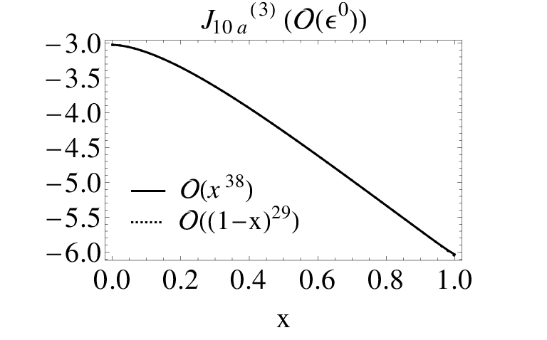
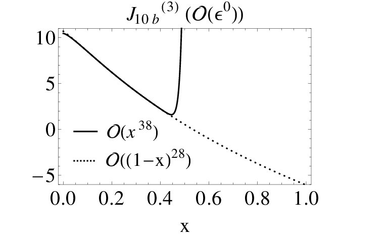
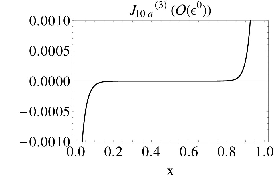
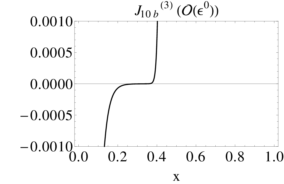
A more precise result for $J^{(3)}_{10a}$ and $J^{(3)}_{10b}$ which is furthermore simpler to handle can be obtained with the help of expansions around $x=0$ and $x=1$ . In contrast to Ref. [22] where expansions of the whole correlator have been considered and thus the expansion depth was limited to 8 and 9 terms, respectively, in this paper results up to order $x^{38}$ and $(1-x)^{28}$ could be obtained for the scalar integrals $J^{(3)}_{10a}$ and $J^{(3)}_{10b}$ .⁴⁴ 4 Note that there are cancellations when constructing the physical moments using the expansion around $x=1$ . Thus some of the moments are only known up to order $(1-x)^{15}$ . The upper plots in Fig. 4 show the results for $J^{(3)}_{10a}$ and $J^{(3)}_{10b}$ using the expansions around $x=0$ (solid) and $x=1$ (dotted). The difference of these results is shown in the bottom plots. One observes perfect agreement over a wide range of $x$ for $J^{(3)}_{10a}$ . In the case of $J^{(3)}_{10b}$ good agreement is only found for $0.2\leq x\leq 0.4$ which suggests to use the $x\to 0$ results for $x<0.3$ and the $x\to 1$ expressions for $x>0.3$ . This has been implemented in the program for the numerical evaluation of the master integrals.

The divergent parts of $J^{(3)}_{10a}$ and $J^{(3)}_{10b}$ can be obtained in analytical form with the help of an asymptotic expansion. They read

	$\displaystyle J^{(3)}_{10a}$	$\displaystyle=$	$\displaystyle{\cal N}^{3}\,\frac{2\zeta_{3}}{\epsilon}+{\cal O}(\epsilon^{0})\,,$		(21)
	$\displaystyle J^{(3)}_{10b}$	$\displaystyle=$	$\displaystyle{\cal N}^{3}\,\frac{2\zeta_{3}}{\epsilon}+{\cal O}(\epsilon^{0})\,.$		(22)

Also for these integrals the order $\epsilon^{1}$ terms do not enter the final results. Thus numerical expressions are only needed for the finite contributions to the moments whereas the cancellation of the poles can be checked analytically.

All available information about the master integrals is provided in the above mentioned Mathematica file TwoMassTadpoles.m [45].

3 Results

3.1 Moments

In this Section we present numerical results for the first four moments of the vector, axial-vector, scalar and pseudo-scalar current correlators. We adapt the colour factors to $SU(3)$ and set the number of massless quarks to three. Furthermore, we set the renormalization scale to $m_{1}$ . More general results that still contain the invariants of $SU(N_{c})$ and labels for the light and heavy quarks can be found in the Mathematica file coefhl2.m [45].

For comparison we also show in Figs. 5 to 8 the results obtained in Ref. [22] as dashed lines. In Ref. [22] expansions around $x=0$ and $x=1$ have been computed which showed good convergence properties up to $x\;\hbox to0.0pt{\lower 3.5pt\hbox{$\mathchar 0\sim$}\hss}\raise 1.0pt\hbox{$<$}\;0.1$ and $x\;\hbox to0.0pt{\lower 3.5pt\hbox{$\mathchar 0\sim$}\hss}\raise 1.0pt\hbox{$>$}\;0.5$ , respectively. Inbetween an interpolation has been performed.

In most cases good agreement is found. Small deviations for $x\approx 0.2\ldots 0.3$ are observed for $\bar{C}_{4}^{(2),v}$ and, to a lesser extent, also for $\bar{C}_{3}^{(2),v}$ , $\bar{C}_{3}^{(2),a}$ , $\bar{C}_{4}^{(2),a}$ , and $\bar{C}_{4}^{(2),s}$ . They demonstrate the importance of the calculation performed in this paper.

From the webpage [45] it is possible to download a Mathematica file which provides the results for all moments of Figs. 5 to 8. Furthermore, also the results for $\bar{C}_{n}^{(2),\delta}$ with $n=-1$ and $n=0$ and for $\bar{C}_{L,n}^{v}$ and $\bar{C}_{L,n}^{a}$ with $n=-1,\ldots,4$ are included. The one- and two-loop expressions are available up to $n=9$ .

3.2 $\rho$ parameter

In this section we discuss an immediate application of $C^{\delta}_{-1}$ of the vector and axial-vector current, namely the QCD corrections to the electroweak $\rho$ parameter which is given by

\displaystyle\rho=1+\delta\rho\,,

(23)

with

\displaystyle\delta\rho=\frac{\Sigma_{Z}(0)}{M_{Z}^{2}}-\frac{\Sigma_{W}(0)}{M_{W}^{2}}\,.

(24)

$\Sigma_{W}(0)$ and $\Sigma_{Z}(0)$ are the transverse parts of the $W$ and $Z$ boson propagators defined through

\displaystyle\Sigma_{W/Z}(0)

\displaystyle=

\displaystyle\frac{g_{\mu\nu}}{d}\,\Pi_{W/Z}^{\mu\nu}\,,

(25)

where $\Pi_{W/Z}^{\mu\nu}$ are the corresponding polarization functions. The QCD corrections to $\delta\rho$ in the Standard Model (SM), where all quark masses except the top quark mass are set to zero, are known up to four loops [49, 50, 51, 52, 25, 23, 24]. In the following we consider a generic fourth generation of quarks which couples to the $W$ and $Z$ boson in the same way as the top and bottom quarks of the SM. For simplicity we denote the new doublet by $(t^{\prime},b^{\prime})$ .

$\Sigma_{W}(0)$ can be obtained from $\bar{C}_{-1}^{v}$ and $\bar{C}_{-1}^{a}$ via the relation

\displaystyle\frac{\Sigma_{W}(0)}{M_{W}^{2}}

\displaystyle=

\displaystyle\frac{3G_{F}m_{t^{\prime}}^{2}}{16\pi^{2}\sqrt{2}}\left(\bar{C}_{-1}^{v}(x)+\bar{C}_{-1}^{a}(x)\right)\,.

(26)

In the case of $\Sigma_{Z}(0)$ there is no contribution form the vector part. Furthermore one has to consider additional contributions at three-loop order which are only present for currents where $\psi_{1}=\psi_{2}$ in Eq. (2). Thus we cast the $Z$ -boson self energy in the form

\displaystyle\frac{\Sigma_{Z}(0)}{M_{Z}^{2}}

\displaystyle=\frac{3G_{F}m_{t^{\prime}}^{2}}{16\pi^{2}\sqrt{2}}\left(\bar{C}_{-1,\rm{diag}}^{a}+\left(\frac{\alpha_{s}}{\pi}\right)^{2}\delta\bar{C}_{-1,\rm{db}}^{a,(2)}+\left(\frac{\alpha_{s}}{\pi}\right)^{2}\delta\bar{C}_{-1,\rm{sing}}^{a,(2)}\right)\,,

(27)

where the quantities $\delta\bar{C}_{-1,\rm db}^{a,(2)}$ and $\delta\bar{C}_{-1,\rm sing}^{a,(2)}$ receive contributions from the double bubble and singlet Feynman diagrams involving two mass scales (see Fig. 9). The double bubble diagrams involving only one massive quark are contained in $\bar{C}_{-1,\rm{diag}}^{a}$ together with all other one-scale contributions. Note that the singlet-type contributions involving massless up, down, strange and charm quarks add up to zero.

In Appendix A explicit analytical results are presented for $\bar{C}_{-1,\rm{diag}}^{a}$ , $\delta\bar{C}_{-1,\rm db}^{a,(2)}$ and $\delta\bar{C}_{-1,\rm sing}^{a,(2)}$ . Let us mention that the treatment of $\gamma_{5}$ for the singlet diagrams can be found in Ref. [53].

Before presenting results we transform the $\overline{\rm MS}$ quark masses $m_{t^{\prime}}$ and $m_{b^{\prime}}$ to the on-shell scheme [54, 55] since this is common practice in the context of analyzing electroweak precision data. For $M_{b^{\prime}}=0$ we reproduce the SM result [51, 52]. The general result can be cast in the form

\displaystyle\delta\rho_{\textrm{OS}}

\displaystyle=\frac{3G_{F}M_{t^{\prime}}^{2}}{16\pi^{2}\sqrt{2}}\Bigg\{2(1+X^{2})+\frac{8\,X^{2}}{1-X^{2}}\,\textrm{H}_{0}(X)+\frac{\alpha_{s}}{\pi}\Delta^{(1)}(X)+\left(\frac{\alpha_{s}}{\pi}\right)^{2}\Delta^{(2)}(X)\Bigg\}\,,

(28)

with $X=M_{b^{\prime}}/M_{t^{\prime}}$ being the ratio of the on-shell quark masses. The two-loop result reads

	$\displaystyle\Delta^{(1)}$	$\displaystyle=\frac{16}{3}\left[-\frac{3}{12}\left(1+X^{2}\right)+\frac{X^{2}}{1-X^{2}}\,\textrm{H}_{0}(X)+\frac{2X^{2}\,\left(3+X^{4}\right)}{\left(1-X^{2}\right)^{2}}\,\textrm{H}_{0,0}(X)\right.$
		$\displaystyle\left.-\left(1-X^{2}\right)\left(\frac{\pi^{2}}{12}+H_{1,0}(X)-H_{-1,0}(X)\right)\right]\,,$		(29)

which agrees with the findings of Ref. [56]. Using the asymptotically expanded master integrals we obtain a series expansion in $X$ and $1-X$ . The results including terms of order $X^{2}$ and $(1-X)^{4}$ read

$\displaystyle\Delta^{(2)}(X)$	$\displaystyle=\frac{85}{324}-\frac{D_{3}}{9}-\frac{2845\pi^{2}}{486}+\frac{26\pi^{4}}{135}+\frac{441S_{2}}{4}-\frac{4}{9}\pi^{2}l_{2}+\frac{4}{27}\pi^{2}l_{2}^{2}$
	$\displaystyle\quad-\frac{4l_{2}^{4}}{27}-\frac{32}{9}a_{4}-\frac{664\zeta_{3}}{27}+n_{l}\left(-\frac{1}{9}+\frac{13\pi^{2}}{27}-\frac{8\zeta_{3}}{9}\right)-X\ \frac{2\pi^{2}}{3}+X^{2}\Bigg[\frac{1943}{81}$
	$\displaystyle\quad+\frac{535\pi^{2}}{972}-\frac{\pi^{4}}{6}+\frac{1125S_{2}}{4}-\frac{4}{9}\pi^{2}l_{2}+\frac{4}{27}\pi^{2}l_{2}^{2}-\frac{4l_{2}^{4}}{27}+\frac{1154l_{X}^{2}}{9}-\frac{304l_{X}^{3}}{9}$
	$\displaystyle\quad-\frac{32}{9}a_{4}+l_{X}\left(\frac{82}{9}-\frac{32\pi^{2}}{9}+\frac{128}{9}\pi^{2}l_{2}-16\pi^{2}l_{2}-\frac{4\zeta_{3}}{3}\right)+n_{l}\left(-\frac{5}{3}+\frac{7\pi^{2}}{27}\right.$
	$\displaystyle\left.\quad+\left(-\frac{4}{3}+\frac{8\pi^{2}}{9}\right)l_{X}-\frac{52l_{X}^{2}}{9}+\frac{32l_{X}^{3}}{9}+\frac{8\zeta_{3}}{9}\right)-\frac{1651\zeta_{3}}{27}\Bigg]+\mathcal{O}(X^{3})\,,$	(30)

where $l_{X}=\log X$ and $\mu^{2}=M_{t^{\prime}}^{2}$ has been adopted⁵⁵ 5 Results for general $\mu$ can be found in rho.m [45]. and

$\displaystyle a_{4}$	$\displaystyle=$	$\displaystyle\mbox{Li}_{4}(1/2)\,\,\approx\,\,0.51747906167389938633\,,$
$\displaystyle S_{2}$	$\displaystyle=$	$\displaystyle\frac{4}{9\sqrt{3}}\mbox{Im}(\mbox{Li}_{2}(e^{i\pi/3}))\,\,\approx\,\,0.26043413763216209896\,,$
$\displaystyle D_{3}$	$\displaystyle=$	$\displaystyle 6\zeta_{3}-\frac{15}{4}\zeta_{4}-6[\mbox{Im}(\mbox{Li}_{2}(e^{i\pi/3}))]^{2}\,\,\approx\,\,-3.0270094939876520198\,.$	(31)

Similarly, the expansion around $M_{b^{\prime}}\approx M_{t^{\prime}}$ leads to

$\displaystyle\Delta^{(2)}(X)$	$\displaystyle=(1-X)^{2}\left[-\frac{5933}{108}-\frac{16}{27}\pi^{2}l_{2}+\frac{2807\zeta_{3}}{72}+n_{l}\left(-\frac{38}{27}+\frac{8\pi^{2}}{27}\right)\right]$
	$\displaystyle\quad+(1-X)^{3}\left(-\frac{116}{9}+\frac{8n_{l}}{9}\right)$
	$\displaystyle\quad+(1-X)^{4}\left[-\frac{465547}{4860}+\frac{4\pi^{2}}{135}+\frac{4}{135}\pi^{2}l_{2}+\frac{157781\zeta_{3}}{2160}+n_{l}\left(\frac{473}{810}-\frac{2\pi^{2}}{135}\right)\right]$
	$\displaystyle\quad+\mathcal{O}((1-X)^{5})\,.$	(32)

In the file rho.m [45] analytical results up to order $X^{30}$ and $(1-X)^{20}$ are provided.

In the above equations $n_{l}$ labels the number of massless quark flavours. In order to reproduce the SM result with massless bottom quark one has $n_{l}=4$ and $x=0$ . The contribution of a fourth generation is obtained for $n_{l}=6$ which assumes a massless top quark at three-loop order.

In the SM the higher order corrections to the $\rho$ parameter are quite important. E.g., the three-loop corrections correspond to a shift in the top quark mass of about 2 GeV which is larger than the current experimental uncertainty. In the limit of equal quark masses $\delta\rho$ is proportional to the mass difference and thus the numerical impact of the higher order corrections is reduced as can be seen from Eq. (32).

4 Summary

In this paper moments of correlators formed by vector, axial-vector, scalar and pseudo-scalar currents are considered to three-loop order. The currents couple to quarks with different masses $m_{1}$ and $m_{2}$ which leads to two-scale vacuum integrals after expanding in the external momentum of the correlators. The moments can be expressed as a linear combination of 12 non-trivial three-loop master integrals which are discussed in details in Section 2. In particular, a Mathematica package TwoMassTadpoles.m is provided [45] which contains analytical results for all but six master integrals. For the latter high-precision numerical results are available. In a further Mathematica file coefhl2.m we also provide results for the first four moments for each correlator.

As a by-product we compute three-loop corrections to the $\rho$ parameter for a generic fourth generation of quarks with masses $m_{t^{\prime}}$ and $m_{b^{\prime}}$ for the up- and down-type quark. In addition to the calculation for the moments of the non-diagonal correlators one has to compute double-bubble and singlet-type diagrams where two different masses can be present in the fermion triangles. For the latter analytical results are provided; the complete results for the $\rho$ parameter up to three loops is available in rho.m [45].

Acknowledgments

This work was supported by the BMBF through Grant No. 05H09VKE and the Graduiertenkolleg “Elementarteilchenphysik bei höchster Energie und höchster Präzision”.

Appendix A Appendix: Explicit results for $\bar{C}_{-1,\rm{diag}}^{a}$ , $\delta\bar{C}_{-1,\rm db}^{a,(2)}$ and $\delta\bar{C}_{-1,\rm sing}^{a,(2)}$

In this appendix analytical results are provided for the building blocks of $\Sigma_{Z}(0)$ in Eq. (27) using the $\overline{\rm MS}$ definition of the quark masses. For convenience we choose for the renormalization scale $\mu^{2}=m_{1}^{2}$ ; general results are available in electronic form from Ref. [45]. Defining

\displaystyle\bar{C}_{-1,\rm{diag}}^{a}

\displaystyle=

\displaystyle\bar{C}_{-1,\rm{diag}}^{a,(0)}+\frac{\alpha_{s}}{\pi}\bar{C}_{-1,\rm{diag}}^{a,(1)}+\left(\frac{\alpha_{s}}{\pi}\right)^{2}\bar{C}_{-1,\rm{diag}}^{a,(2)}\,,

(33)

we have

$\displaystyle\bar{C}_{-1,\rm{diag}}^{a,(0)}$	$\displaystyle=-\frac{4\left(1+x^{2}\right)}{\epsilon}+8x^{2}\textrm{H}_{0}(x)\,,$
$\displaystyle\bar{C}_{-1,\rm{diag}}^{a,(1)}$	$\displaystyle=\frac{4\left(1+x^{2}\right)}{\epsilon^{2}}-\frac{10\left(1+x^{2}\right)}{3\epsilon}+\frac{1}{3}\left(-1-x^{2}\right)-\frac{8}{3}x^{2}\textrm{H}_{0}(x)-32x^{2}\textrm{H}_{0,0}(x)\,,$
$\displaystyle\bar{C}_{-1,\rm{diag}}^{a,(2)}$	$\displaystyle=\frac{1}{\epsilon^{3}}\left(-\frac{19}{3}\left(1+x^{2}\right)\right)+\frac{1}{\epsilon^{2}}\left(\frac{281}{18}\left(1+x^{2}\right)+\frac{8}{3}x^{2}\textrm{H}_{0}(x)\right)$
	$\displaystyle\quad+\frac{1}{\epsilon}\Big(-\frac{4}{3}x^{2}\textrm{H}_{0}(x)-16x^{2}\textrm{H}_{0,0}(x)-\frac{1}{54}\left(1+x^{2}\right)\left(401+6\pi^{2}\right.$
	$\displaystyle\left.\quad-36\zeta_{3}\right)\Big)+\frac{1}{18}x^{2}\textrm{H}_{0}(x)\left(-181+12\pi^{2}-72\zeta_{3}\right)-\frac{272}{9}x^{2}\textrm{H}_{0,0}(x)$
	$\displaystyle\quad+\frac{1136}{3}x^{2}\textrm{H}_{0,0,0}(x)-\frac{1}{90}\left(1+x^{2}\right)\Big(-790+\left(-5+40l_{2}^{2}\right)\pi^{2}+\frac{22}{3}\pi^{4}-40l_{2}^{4}$
	$\displaystyle\quad+1160\zeta_{3}-960a_{4}\Big)+n_{l}\Bigg(\frac{2\left(1+x^{2}\right)}{9\epsilon^{3}}-\frac{5\left(1+x^{2}\right)}{9\epsilon^{2}}+\frac{4\left(1+x^{2}\right)}{9\epsilon}-\frac{5}{9}x^{2}\textrm{H}_{0}(x)$
	$\displaystyle\quad+\frac{32}{9}x^{2}\textrm{H}_{0,0}(x)-\frac{32}{3}x^{2}\textrm{H}_{0,0,0}(x)+\frac{1}{18}\left(1+x^{2}\right)(-1+32\zeta_{3})\Bigg)\,.$	(34)

The double bubble and singlet result is given by

$\displaystyle\delta\bar{C}_{-1,\mathrm{db}}^{a,(2)}$	$\displaystyle=\frac{4\left(1+x^{2}\right)}{9\epsilon^{3}}+\frac{-\frac{2}{9}\left(1+x^{2}\right)-\frac{8}{3}x^{2}\textrm{H}_{0}(x)}{\epsilon^{2}}$
	$\displaystyle\quad+\frac{\frac{1}{9}\left(-1+\pi^{2}\right)\left(1+x^{2}\right)+\frac{4}{3}x^{2}\textrm{H}_{0}(x)+16x^{2}\textrm{H}_{0,0}(x)}{\epsilon}$
	$\displaystyle\quad+\frac{2}{3}\left(2-\left(1+\pi^{2}\right)x^{2}\right)\textrm{H}_{0}(x)-\frac{4}{3}\left(1+7x^{2}\right)\textrm{H}_{0,0}(x)$
	$\displaystyle\quad+\frac{2\left(1-8x-6x^{2}-8x^{3}+x^{4}\right)\textrm{H}_{-1,0,0}(x)}{3x}$
	$\displaystyle\quad-\frac{256}{3}x^{2}\textrm{H}_{0,0,0}(x)+\frac{2\left(1+8x-6x^{2}+8x^{3}+x^{4}\right)\textrm{H}_{1,0,0}(x)}{3x}$
	$\displaystyle\quad-\frac{1}{18}\left(1+x^{2}\right)\left(49+\pi^{2}-38\zeta_{3}\right)\,,$
$\displaystyle\delta\bar{C}_{-1,\mathrm{sing}}^{a,(2)}$	$\displaystyle=8x\left(\textrm{H}_{1,0,0}(x)+\textrm{H}_{-1,0,0}(x)\right)-7\left(1+x^{2}\right)\zeta_{3}\,.$	(35)

The three-loop result $\bar{C}_{-1,\rm{diag}}^{a,(2)}$ depends on the number of massless flavours $n_{l}$ . Let us finally mention that the Mathematica package rho.m contains replacement rules which express the HPLs occurring in Eqs. (34) and (35) in terms of logarithms and dilogarithms.

References

[1] P. A. Baikov, K. G. Chetyrkin and J. H. Kühn, Phys. Rev. Lett. 101 (2008) 012002 [arXiv:0801.1821 [hep-ph]].
[2] P. A. Baikov, K. G. Chetyrkin, J. H. Kühn and J. Rittinger, arXiv:1201.5804 [hep-ph].
[3] A. O. G. Kallen and A. Sabry, Kong. Dan. Vid. Sel. Mat. Fys. Med. 29N17 (1955) 1.
[4] K. G. Chetyrkin, J. H. Kühn and M. Steinhauser, Nucl. Phys. B 482 (1996) 213 [arXiv:hep-ph/9606230].
[5] K. G. Chetyrkin, J. H. Kühn and M. Steinhauser, Nucl. Phys. B 505 (1997) 40 [arXiv:hep-ph/9705254].
[6] A. Maier, P. Maierhofer and P. Marquard, Nucl. Phys. B 797 (2008) 218 [arXiv:0711.2636 [hep-ph]].
[7] K. G. Chetyrkin, J. H. Kühn and C. Sturm, Eur. Phys. J. C 48 (2006) 107 [arXiv:hep-ph/0604234].
[8] R. Boughezal, M. Czakon and T. Schutzmeier, Phys. Rev. D 74 (2006) 074006 [arXiv:hep-ph/0605023].
[9] C. Sturm, JHEP 0809 (2008) 075 [arXiv:0805.3358 [hep-ph]].
[10] A. Maier, P. Maierhofer and P. Marquard, Phys. Lett. B 669 (2008) 88 [arXiv:0806.3405 [hep-ph]].
[11] Y. Kiyo, A. Maier, P. Maierhofer and P. Marquard, Nucl. Phys. B 823 (2009) 269 [arXiv:0907.2120 [hep-ph]].
[12] J. H. Kühn, M. Steinhauser and C. Sturm, Nucl. Phys. B 778 (2007) 192 [arXiv:hep-ph/0702103].
[13] I. Allison et al. [HPQCD Collaboration], Phys. Rev. D 78 (2008) 054513 [arXiv:0805.2999 [hep-lat]].
[14] K. G. Chetyrkin, J. H. Kühn, A. Maier, P. Maierhofer, P. Marquard, M. Steinhauser and C. Sturm, Phys. Rev. D 80 (2009) 074010 [arXiv:0907.2110 [hep-ph]].
[15] C. McNeile, C. T. H. Davies, E. Follana, K. Hornbostel and G. P. Lepage, Phys. Rev. D 82 (2010) 034512 [arXiv:1004.4285 [hep-lat]].
[16] K. Chetyrkin, J. H. Kühn, A. Maier, P. Maierhofer, P. Marquard, M. Steinhauser and C. Sturm, arXiv:1010.6157 [hep-ph].
[17] A. Djouadi and P. Gambino, Phys. Rev. D 49 (1994) 3499 [Erratum-ibid. D 53 (1996) 4111] [arXiv:hep-ph/9309298].
[18] A. Djouadi and P. Gambino, Phys. Rev. D 51 (1995) 218 [Erratum-ibid. D 53 (1996) 4111] [arXiv:hep-ph/9406431].
[19] K. G. Chetyrkin and M. Steinhauser, Phys. Lett. B 502 (2001) 104 [arXiv:hep-ph/0012002].
[20] K. G. Chetyrkin and M. Steinhauser, Eur. Phys. J. C 21 (2001) 319 [arXiv:hep-ph/0108017].
[21] A. Maier and P. Marquard, Nucl. Phys. B 859 (2012) 1 [arXiv:1110.5581 [hep-ph]].
[22] J. Hoff and M. Steinhauser, Nucl. Phys. B 849 (2011) 610 [arXiv:1103.1481 [hep-ph]].
[23] K. G. Chetyrkin, M. Faisst, J. H. Kühn, P. Maierhofer and C. Sturm, Phys. Rev. Lett. 97 (2006) 102003 [hep-ph/0605201].
[24] R. Boughezal and M. Czakon, Nucl. Phys. B 755 (2006) 221 [hep-ph/0606232].
[25] Y. Schröder and M. Steinhauser, Phys. Lett. B 622 (2005) 124 [arXiv:hep-ph/0504055].
[26] J. Koponen et al. [HPQCD Collaboration], arXiv:1011.1208 [hep-lat].
[27] K. G. Chetyrkin, J. H. Kühn and A. Kwiatkowski, Phys. Rept. 277 (1996) 189.
[28] P. Nogueira, J. Comput. Phys. 105 (1993) 279.
[29] J. A. M. Vermaseren, arXiv:math-ph/0010025.
[30] J. Kuipers, T. Ueda, J. A. M. Vermaseren and J. Vollinga, arXiv:1203.6543 [cs.SC].
[31] R. Harlander, T. Seidensticker and M. Steinhauser, Phys. Lett. B 426 (1998) 125, arXiv:hep-ph/9712228.
[32] T. Seidensticker, arXiv:hep-ph/9905298.
[33] A. V. Smirnov, JHEP 0810 (2008) 107 [arXiv:0807.3243 [hep-ph]].
[34] A. I. Davydychev and J. B. Tausk, Nucl. Phys. B 397 (1993) 123.
[35] Y. Schröder and A. Vuorinen, JHEP 0506 (2005) 051 [hep-ph/0503209].
[36] A. V. Kotikov, Phys. Lett. B 267 (1991) 123.
[37] E. Remiddi, Nuovo Cim. A 110 (1997) 1435 [hep-th/9711188].
[38] M. Caffo, H. Czyz, S. Laporta and E. Remiddi, Nuovo Cim. A 111 (1998) 365 [hep-th/9805118].
[39] T. Gehrmann and E. Remiddi, Nucl. Phys. B 580 (2000) 485 [hep-ph/9912329].
[40] M. Argeri and P. Mastrolia, Int. J. Mod. Phys. A 22 (2007) 4375 [arXiv:0707.4037 [hep-ph]].
[41] S. Bekavac, A. G. Grozin, D. Seidel and V. A. Smirnov, Nucl. Phys. B 819 (2009) 183 [arXiv:0903.4760 [hep-ph]].
[42] E. Remiddi and J. A. M. Vermaseren, Int. J. Mod. Phys. A 15 (2000) 725 [hep-ph/9905237].
[43] D. Maitre, Comput. Phys. Commun. 174 (2006) 222 [hep-ph/0507152].
[44] D. Maitre, Comput. Phys. Commun. 183 (2012) 846 [hep-ph/0703052 [HEP-PH]].
[45] www-ttp.particle.uni-karlsruhe.de/Progdata/ttp12/ttp12-20/
[46] V. A. Smirnov, Phys. Lett. B 460 (1999) 397 [hep-ph/9905323].
[47] J. B. Tausk, Phys. Lett. B 469 (1999) 225 [hep-ph/9909506].
[48] M. Czakon, Comput. Phys. Commun. 175 (2006) 559 [hep-ph/0511200].
[49] M. J. G. Veltman, Nucl. Phys. B 123 (1977) 89.
[50] A. Djouadi, Nuovo Cim. A 100 (1988) 357.
[51] K. G. Chetyrkin, J. H. Kühn and M. Steinhauser, Phys. Lett. B 351 (1995) 331 [hep-ph/9502291].
[52] L. Avdeev, J. Fleischer, S. Mikhailov and O. Tarasov, Phys. Lett. B 336 (1994) 560 [Erratum-ibid. B 349 (1995) 597] [hep-ph/9406363].
[53] S. A. Larin, Phys. Lett. B 303 (1993) 113 [hep-ph/9302240].
[54] N. Gray, D. J. Broadhurst, W. Grafe and K. Schilcher, Z. Phys. C 48 (1990) 673.
[55] S. Bekavac, A. Grozin, D. Seidel and M. Steinhauser, JHEP 0710 (2007) 006 [arXiv:0708.1729 [hep-ph]].
[56] A. Djouadi and P. Gambino, Phys. Rev. D 49 (1994) 4705 [hep-ph/9308338].


(a)	(b)

SFB/CPP-12-39 TTP12-20 Moments of heavy quark correlators with two masses: exact mass dependence to three loops

Abstract

1 QCD corrections to current correlators

2 Master integrals for non-diagonal correlators

2.1 Differential equation method

2.2 J5​a(3)J^{(3)}_{5a}, J5​b(3)J^{(3)}_{5b}, J6​a(3)J^{(3)}_{6a} and J6​b(3)J^{(3)}_{6b}

2.3 J1(3)J^{(3)}_{1}, J2(3)J^{(3)}_{2}, J3(3)J^{(3)}_{3}, J4(3)J^{(3)}_{4}, J7​a(3)J^{(3)}_{7a} and J7​b(3)J^{(3)}_{7b}

2.4 J8​a(3)J^{(3)}_{8a}, J8​b(3)J^{(3)}_{8b}, J9​a(3)J^{(3)}_{9a} and J9​b(3)J^{(3)}_{9b}

2.5 J10​a(3)J^{(3)}_{10a} and J10​b(3)J^{(3)}_{10b}