Astroclimate at San Pedro Mártir I: 2004 – 2008 Seeing Statistics from the TMT Site Testing DataThanks: Based on observations obtained at the Observatorio Astronómico Nacional at San Pedro Mártir, Baja California, México, operated by the Instituto de Astronomía, Universidad Nacional Autónoma de México.
Abstract
We present comprehensive seeing statistics for the San Pedro Mártir site derived from the Thirty Meter Telescope site selection data. The observations were obtained between 2004 and 2008 with a Differential Image Motion Monitor (DIMM) and a Multi Aperture Scintillation Sensor (MASS) combined instrument (MASS - DIMM). The parameters that are statistically analised here are: whole atmosphere seeing measured by the DIMM; free atmosphere seeing -measured by the MASS-; and ground-layer seeing (GL) -difference between the total and free-atmosphere seeing-. We made a careful data coverage study along with statistical distributions of simultaneous MASS - DIMM seeing measurements, in order to investigate the nightly, monthly, seasonal, annual and global behaviour, as well as possible hourly seeing trends. Although this campaign covers five years, the sampling is uneven, being 2006 and 2007 the best sampled years in terms of seasonal coverage. The overall results yield a median seeing of 0.78 (DIMM), 0.37 (MASS) and 0.59 arcsec (GL). The strongest contribution to the whole atmosphere seeing comes, therefore, from a strong ground layer. We find that the best season is summer, while the worst one is winter, in accordance with previous studies. It is worth noting that the best yearly results are correlated with the best sampled years. The hourly analysis shows that there is no statistically significant tendency of seeing degradation towards dawn. The seeing values are slightly larger than those reported before. This may be caused by climate changes.
Keywords:
atmospheric effects – site testing1 Introduction
In the early seventies a new observing site began operations at the Sierra de San Pedro Mártir (SPM), Baja California, México. The site was selected through satellite photographs, and was found to be one of the three best cloud-free areas in the world.
We now know that this site is one of the best astronomical locations in the world and has been considered by the international astronomical community as a potential place for large telescopes to be built in the near future being a candidate site of projects such as the Large Synoptic Survey Telescope (LSST) and the Thirty Meter Telescope (TMT), as well as other astronomical projects.
Several climatological properties have been reported, mainly during the first years of operation of the Observatorio Astronómico Nacional (OAN) at SPM (Mendoza, 1971; Mendoza, 1973; Mendoza et al., 1972; Alvarez & Maisterrena, 1977; Alvarez & López, 1982; Walker, 1984) and later by Tapia (1992); Tapia (2003); Echevarría et al. (1998); Hiriart et al. (2001); Michel et al. (2003c); Michel et al. (2003a); Carrasco & Sarazin (2003); Carrasco et al. (2005); Avila et al. (2006); Tapia et al. (2007a); Alvarez et al. (2007); Bohigas et al. (2008); Otárola et al. (2009); Bohigas & Núñez (2010); Araiza Quijano & Cruz-González (2011) and Carrasco et al. (2012).
| Method | 1st Quart. | Median | 3rd Quart. | Nights |
|---|---|---|---|---|
| (arcsec) | (arcsec) | (arcsec) | ||
| STT1 | 0.50 | 0.61 | 386 | |
| CM1 | 0.48 | 0.63 | 99 | |
| CM / STT1,a | 0.46 | 0.58 | 57 | |
| DIMM2 | 0.50; 0.75b | 14 | ||
| DIMM2 | 0.61 | 0.77 | 0.99 | 31 |
| DIMM3 | 0.48 | 0.60 | 0.81 | 123 |
| MASS – DIMM4 | 0.61 | 0.79 | 1.12 | c |
| SciDAR5 | 0.50 | 0.68 | 0.97 | 27 |
1 Echevarría et al. (1998), 2 Conan et al. (2002), 3 Michel et al. (2003a), 4 Skidmore et al. (2009), 5 Avila et al. (2011)
a CM simultaneous with STT, b Bimodal distribution, c (2004 Oct. – 2008 Feb.)
Results on the seeing and optical turbulence above the ground can be found in Avila et al. (1998); Echevarría et al. (1998); Conan et al. (2002); Avila et al. (2007); Sánchez et al. (2007) and Avila et al. (2011), as well as atmosphere modelling by Masciadri & Garfias (2001); Masciadri et al. (2002); Masciadri et al. (2003); Masciadri et al. (2004) and Vogiatzis & Hiriart (2004). Extinction and opacity studies have also been made by Schuster & Parrao (2001); Hiriart (2003) and Parrao & Schuster (2003). Site prospection studies within the SPM site have been made by Sohn (2007) and Bohigas et al. (2008). Comprehensive reviews on the site can be found in Cruz-González et al. (2003); Cruz-González et al. (2004); Tapia et al. (2007a); Tapia et al. (2007b) and Wehinger (2007).
In this article, we analyse the data collected by the TMT Project Site Survey at the SPM site and discuss and compare results of Differential Image Motion Monitor (DIMM) and a Multi Aperture Scintillation Sensor (MASS) with previous studies. The observations include data in the time period 2004 October to 2008 February analysed by Skidmore et al. (2009), plus data taken between 2008 February to 2008 August whose analysis has not been presented anywhere in the astronomical literature, improving considerably the analysis of the complete TMT MASS – DIMM seeing survey at SPM and supplementing previous seeing results published in the literature.
We also present in a detailed manner the number of observations and the percentage of time covered by them. This a novel way of treating seeing data.
In the spirit of providing the astronomical community with detailed information of the seeing behaviour in SPM, we present nightly, monthly, seasonal, annual and global statistics. We too, present an analysis of the hourly seeing trend which yields different results from those found by Skidmore et al. (2009).
2 The SPM Site: Seeing Studies
The atmospheric turbulence is usually studied through a number of parameters, one of which is known as seeing (). The relation between , Fried parameter , and the turbulence integral is given by
| (1) |
where is the wavelength and is the optical turbulence energy profile (Roddier, 1981).
We note that the seeing units are given in arcseconds (arcsec) and since seeing is a wavelength-dependent turbulence parameter it is usually calculated for 0.5 m. The seeing value is also corrected for the direction of observation and is referred to zero zenith angle.
Early works on local SPM seeing conditions were done by Mendoza (1971) and Walker (1971), and several recent studies have been carried out by Echevarría et al. (1998); Conan et al. (2002) and Michel et al. (2003a). Optical turbulence studies have been made by Avila et al. (1998); Avila et al. (2004); Avila et al. (2006); Avila et al. (2007) and Avila et al. (2011). A comprehensive review of some of these studies can be found in Echevarría (2003).
The Echevarría et al. (1998) observations were obtained with two seeing monitors and a Micro Temperature Array tower (MTA); the Site Testing Telescope (STT) from Steward Observatory was designed to observe Polaris, while the Carnegie Monitor (CM) could observe and track any star. The MTA consisted of platinum detectors, which measured temperature differences located at different heights, from 4 to 28 m. These authors report a median seeing of 0.61 arcsec with a first quartile of 0.50 arcsec and a decrease of 0.1 arcsec at a height of 15 m. The STT observations covered 386 nights, while the CM observations covered 114 nights, spanning a three year period. A summary of their results is shown in Table 1.
Conan et al. (2002) measured the wavefront outer scale and included ground-based seeing measurements with a DIMM monitor. They reported observations during 31 nights. The telescope was located at two sites: at the CM tower and at a low altitude location. In their article they found a bimodal distribution during their 2000 December campaign with peaks centred at 0.50 and 0.75 arcsec, and an overall seeing median of 0.77 arcsec including all observations during the 31-night period.
Michel et al. (2003a) conducted a study with the same DIMM monitor during 123 nights spanning almost a three year period. The monitor was located at the CM tower at a height of 8.3 m. These authors reported a median of 0.62 arcsec and a first quartile of 0.49 arcsec.
Skidmore et al. (2009) analyse data collected by the TMT Project Site Survey at five different sites which include SPM. A partial set (2004 Oct. to 2008 Feb.), of combined DIMM and MASS data, yields seeing median values for the ground layer 0.58 arcsec, for the free atmosphere 0.37 arcsec and for the whole atmosphere 0.79 arcsec.
Concerning optical turbulence profiling, Avila et al. (1998); Avila et al. (2004) monitored the vertical distribution of the optical turbulence strength using a Generalized SciDAR (GS). Two observation campaigns have been carried out at the OAN – SPM in 1997 and 2000. In 1997, the GS was installed at the 1.5 m and 2.1 m telescopes (SPM1.5 and SPM2.1) for 8 and 3 nights (March and April), respectively, whereas in 2000 the instrument was installed for 9 and 7 nights (May) at SPM1.5 and SPM2.1, respectively.
Avila et al. (2011) performed a recalibration of the profiles obtained in the OAN – SPM, following the results of a theoretical work on the normalization procedure used in the GS data reduction method (Avila & Cuevas, 2009). From a statistical analysis of the recalibrated profiles, Avila et al. (2011) have found that the seeing in the first two kilometers, in the free atmosphere, and in the whole atmosphere had median values of 0.38, 0.35 and 0.68 arcsec, respectively.
A synthesis of the non-differential monitors (STT & CM), differential (DIMM) and SciDAR seeing monitoring campaigns is shown in Table 1.
3 TMT Site Testing Data
3.1 The 2004 – 2008 TMT site testing campaign
SPM was one of the five candidate sites selected by the TMT site testing team (Schöck et al., 2009). Three southern hemisphere sites were studied, Cerros Tolar, Armazones and Tolonchar in northern Chile, and two northern hemisphere sites, the 13 North (13 N) site on Mauna Kea, Hawaii in the United States and SPM in Mexico. During a period of approximately five years, from 2004 to 2008, the TMT group measured the atmospheric properties of each site with the same instrumentation and at least 2.5 annual cycles of data were acquired on each of the candidate sites. As is described in detail by Schöck et al. (2009) a suite of eight instruments were deployed in the candidate sites. The data acquisition methodology is also presented in their work. The acquired data of all the instruments is kindly available to the public at http://sitedata.tmt.org/ by the TMT organisation.

| Year | ||||||||||||
| Month | 2004 | 2005 | 2006 | 2007 | 2008 | Total | ||||||
| January | – | – | 129 | 0.9 % | 3371 | 23.1 % | 6263 | 43.1 % | 0 | 0.0 % | 9763 | 16.8 % |
| February | – | – | 0 | 0.0 % | 3082 | 23.5 % | 7767 | 60.9 % | 4449 | 35.5 % | 15298 | 30.0 % |
| March | – | – | 0 | 0.0 % | 5740 | 46.3 % | 5992 | 47.0 % | 4794 | 38.9 % | 16526 | 33.0 % |
| Winter | 41587 | 26.6 % | ||||||||||
| April | – | – | 2846 | 25.5 % | 8185 | 74.4 % | 3901 | 36.4 % | 9557 | 86.7 % | 24489 | 55.7 % |
| May | – | – | 6755 | 64.9 % | 7640 | 73.5 % | 8472 | 81.5 % | 7657 | 73.6 % | 30524 | 73.4 % |
| June | – | – | 5740 | 59.9 % | 6609 | 69.0 % | 3959 | 41.4 % | 6233 | 65.1 % | 22541 | 58.8 % |
| Spring | 77554 | 62.6 % | ||||||||||
| July | – | – | 628 | 6.3 % | 5064 | 50.3 % | 5792 | 57.7 % | 4155 | 41.2 % | 15639 | 38.9 % |
| August | – | – | 0 | 0.0 % | 6578 | 60.3 % | 6174 | 56.1 % | 642 | 6.1 % | 13394 | 30.6 % |
| September | – | – | 0 | 0.0 % | 8361 | 71.2 % | 0 | 0.0 % | – | – | 8361 | 23.8 % |
| Summer | 37394 | 31.1 % | ||||||||||
| October | 6081 | 45.5 % | 445 | 3.2 % | 8712 | 66.1 % | 8612 | 63.7 % | – | – | 23850 | 44.6 % |
| November | 3887 | 28.0 % | 10134 | 73.6 % | 9916 | 72.1 % | 8004 | 57.7 % | – | – | 31941 | 57.8 % |
| December | 0 | 0.0 % | 5165 | 35.1 % | 5933 | 40.3 % | 0 | 0.0 % | – | – | 11098 | 18.8 % |
| Autumn | 66889 | 40.4 % | ||||||||||
| Total | 9968 | 36.7 % | 31842 | 22.4 % | 79191 | 55.8 % | 64936 | 45.4 % | 37487 | 43.4 % | 223424 | 40.2 % |
| Year | ||||||||||||
| Month | 2004 | 2005 | 2006 | 2007 | 2008 | Total | ||||||
| January | – | – | 241 | 1.7 % | 2663 | 18.2 % | 5768 | 39.7 % | 0 | 0.0 % | 8672 | 14.9 % |
| February | – | – | 0 | 0.0 % | 2448 | 18.7 % | 6451 | 50.6 % | 2536 | 20.3 % | 11435 | 22.4 % |
| March | – | – | 0 | 0.0 % | 4669 | 37.7 % | 4890 | 38.4 % | 354 | 2.7 % | 9913 | 19.7 % |
| Winter | 30020 | 19.0 % | ||||||||||
| April | – | – | 2414 | 21.6 % | 7283 | 66.3 % | 3562 | 33.2 % | 0 | 0.0 % | 13259 | 30.3 % |
| May | – | – | 6164 | 59.1 % | 6846 | 65.9 % | 7366 | 70.9 % | 6106 | 58.7 % | 26482 | 63.6 % |
| June | – | – | 5006 | 52.3 % | 5516 | 57.5 % | 3266 | 34.2 % | 3274 | 34.2 % | 17062 | 44.5 % |
| Spring | 56803 | 46.1 % | ||||||||||
| July | – | – | 463 | 4.6 % | 4509 | 44.8 % | 2294 | 22.8 % | 0 | 0.0 % | 7266 | 18.1 % |
| August | – | – | 0 | 0.0 % | 5816 | 53.3 % | 5837 | 53.6 % | 0 | 0.0 % | 11653 | 26.7 % |
| September | – | – | 0 | 0.0 % | 7641 | 65.2 % | 0 | 0.0 % | – | – | 7641 | 21.7 % |
| Summer | 26560 | 22.2 % | ||||||||||
| October | 5159 | 38.9 % | 336 | 2.5 % | 7223 | 54.7 % | 0 | 0.0 % | – | – | 12718 | 24.0 % |
| November | 3436 | 25.5 % | 7428 | 53.7 % | 6786 | 49.3 % | 263 | 1.9 % | – | – | 17913 | 32.6 % |
| December | 0 | 0.0 % | 3908 | 26.6 % | 4687 | 31.8 % | 0 | 0.0 % | – | – | 8595 | 14.6 % |
| Autumn | 39226 | 23.7 % | ||||||||||
| Total | 8595 | 21.5 % | 25960 | 18.5 % | 66087 | 46.9 % | 39697 | 28.8 % | 12270 | 14.5 % | 152609 | 27.9 % |
| Year | ||||||||||||
| Month | 2004 | 2005 | 2006 | 2007 | 2008 | Total | ||||||
| January | – | – | 63 | 0.4 % | 2613 | 17.9 % | 5451 | 37.5 % | 0 | 0.0 % | 8127 | 14.0 % |
| February | – | – | 0 | 0.0 % | 2394 | 18.2 % | 6152 | 48.3 % | 2490 | 20.0 % | 11036 | 21.6 % |
| March | – | – | 0 | 0.0 % | 4521 | 36.5 % | 4713 | 37.0 % | 352 | 2.7 % | 9586 | 19.1 % |
| Winter | 28749 | 18.2 % | ||||||||||
| April | – | – | 2399 | 21.5 % | 7129 | 64.9 % | 3422 | 31.9 % | 0 | 0.0 % | 12950 | 29.6 % |
| May | – | – | 5779 | 55.4 % | 6707 | 64.5 % | 7156 | 68.9 % | 5946 | 57.2 % | 25588 | 61.5 % |
| June | – | – | 4857 | 50.7 % | 5331 | 55.6 % | 3088 | 32.3 % | 3117 | 32.5 % | 16393 | 42.8 % |
| Spring | 54931 | 44.6 % | ||||||||||
| July | – | – | 340 | 3.4 % | 4134 | 41.0 % | 1751 | 17.6 % | 0 | 0.0 % | 6225 | 15.5 % |
| August | – | – | 0 | 0.0 % | 5625 | 51.5 % | 4511 | 41.1 % | 0 | 0.0 % | 10136 | 23.2 % |
| September | – | – | 0 | 0.0 % | 7360 | 62.8 % | 0 | 0.0 % | – | – | 7360 | 20.9 % |
| Summer | 23721 | 19.9 % | ||||||||||
| October | 4033 | 30.5 % | 337 | 2.5 % | 6941 | 52.6 % | 0 | 0.0 % | – | – | 11311 | 21.4 % |
| November | 3259 | 24.2 % | 7274 | 52.6 % | 6607 | 48.0 % | 241 | 1.7 % | – | – | 17381 | 31.6 % |
| December | 0 | 0.0 % | 3819 | 25.9 % | 4451 | 30.2 % | 0 | 0.0 % | – | – | 8270 | 14.0 % |
| Autumn | 36962 | 22.3 % | ||||||||||
| Total | 7292 | 18.2 % | 24868 | 17.7 % | 63813 | 45.3 % | 36485 | 26.4 % | 11905 | 14.1 % | 144363 | 26.4 % |
3.2 Seeing Instrumentation
The SPM TMT T4 site testing station was equipped with a 35 cm telescope mounted approximately 7 m above ground. At the Cassegrain focus of the telescope a combined instrument was deployed, which included a DIMM and a MASS, hereafter called MASS – DIMM described by Kornilov et al. (2007). Combined MASS – DIMM instruments are extensively used for seeing measurements and optical turbulence profiling (Tokovinin et al., 2003; Tokovinin et al., 2005, e.g.).
The DIMM channel measures the wavefront slope differences over two small pupils some distance apart. This yields the whole atmosphere seeing from the telescope level to the top of the atmosphere (Sarazin & Roddier, 1990). DIMM seeing measurements are affected by different sources of bias such as image threshold, defocus, exposure time, photon noise, and high-frequency vibrations that must be monitored in real time, thus part of the measurements are rejected. In particular, for the system used here, the precision reported is better than 0.02 arcsec (Wang et al., 2007).
The MASS channel detects rapid variations of light intensity in four concentric apertures using photomultipliers and reconstructs a turbulence profile at six different heights above the telescope, (Tokovinin & Kornilov, 2007). MASS is not sensitive to turbulence near the ground as this does not produce any scintillation and it can only measure the seeing in the free atmosphere (FA), thus excluding the ground layer, so we have . From the turbulence profile the seeing integrated from 500 m above the telescope to the top of the atmosphere is computed. MASS seeing accuracy is better than 0.05 arcsec (Els et al., 2008).
3.3 SPM TMT Data Coverage
The SPM TMT T4 station acquired MASS – DIMM data from 2004 October to 2008 August. The DIMM and MASS nightly operations commenced one hour after sunset and ceased one hour before sunrise. DIMM and MASS measurements were triggered simultaneously, DIMM took integrated stellar light measurements during a time interval of 36 s, whereas MASS sampled light during 60 s periods. As the DIMM channel was used to acquire the target star, this resulted in simultaneous MASS – DIMM measurements every 70 to 90 s (Els et al., 2009). Sometimes computations failed to provide valid results probably due to cloudy conditions or technical problems, while sometimes the telescope system was shutdown due to bad weather conditions.
In Fig. 1 we present the total amount of DIMM, MASS and simultaneous MASS – DIMM data for each month during the acquisition period. By simultaneous MASS – DIMM data we mean measurements within the same minute interval.
We have also computed the statistics of the data coverage per night and per month. To compute the monthly temporal data coverage we have considered the duration for each night of the year due to the diurnal cycle variation. This yields a percentage value of the available data for each night in a given month. A 100 % value would indicate data obtained during the whole night for every night of the month.
To our knowledge, this is the first time that a complete data coverage of seeing observations is presented in the astronomical literature. Whereas in other papers it is spoken of number of nights observed regardless of whether one seeing-point or many have been observed per night, we emphasise the effective length of time observed per night; making this a novel way of treating seeing data.
In Tables 2, 3 and 4 we give the percentage of monthly, seasonal and annual data coverage of DIMM, MASS and simultaneous MASS – DIMM during the acquisition period.
In Figs. 2, 3 and 4 we present grey level plots showing only the monthly percentage of data coverage for the 2004 – 2008 period for DIMM, MASS and simultaneous MASS – DIMM, extracted from Tables 2, 3 and 4.
These figures are intended to be a visual aid in order to see, at a glance, which months are those with the best coverage. The degree of darkening corresponds to the monthly percentage values presented in Tables 2, 3 and 4.
At a first glance we immediately notice two main features. First, that the best coverage was obtained during 2006 and 2007; secondly, that April, May and June are the best covered months.
This is further supported by a careful analysis in Tables 2, 3 and 4. For 2006 and 2007 the DIMM data coverage is 55.8 and 45.4 % respectively, while the MASS coverage for these years is 46.9 and 28.8 % respectively. The simultaneous MASS – DIMM coverage is 45.3 and 26.4 % respectively. The overall data coverage for all years is significantly less (DIMM 40.2 %; MASS 27.9 %; and simultaneous MASS – DIMM 26.4 %). Although these coverage values are low they reflect the enormous difficulties in obtaining seeing data, even in experiments designed to ensure high data collection efficiencies, as is the case of the TMT site testing data (Riddle et al., 2006; Schöck et al., 2010). Note that the best sampled year for simultaneous measurements is 2006 (45.3 %) and the worst sampled one is 2008 (14.1 %).


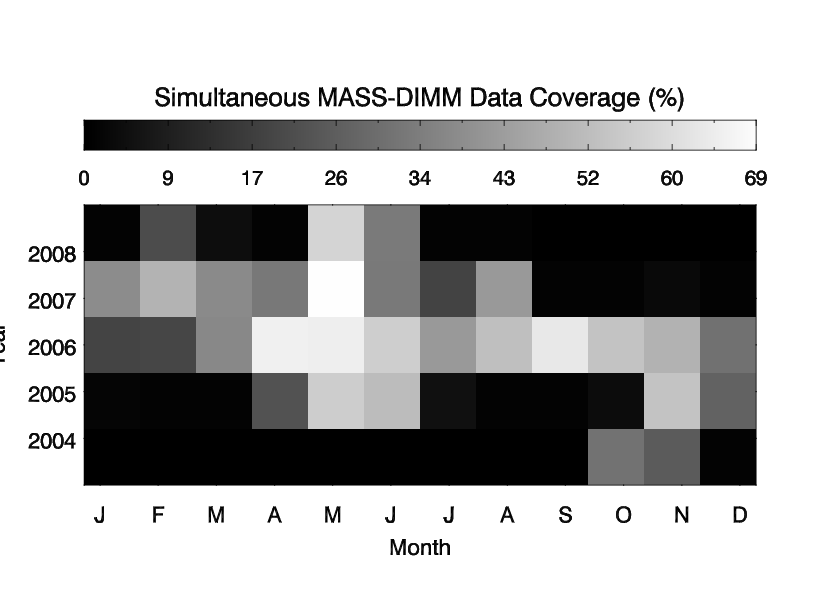
Seasonal MASS – DIMM coverage in winter is 18.2 %, spring 44.6 %, summer 19.9 %, and autumn 22.3 %. Seasons have been defined at the beginning of the month: winter (January, February and March); spring (April, May and June); summer (July, August and September) and autumn (October, November and December).
In the monthly case we can see that the data coverage is worse in January (14.0 %), December (14.0 %) and July (15.5 %), while the best sampled months are May (61.5 %), June (42.8 %) and November (31.6 %).
4 Results
We have calculated the seeing from MASS, DIMM and simultaneous MASS – DIMM obtaining nightly, monthly, seasonal, annual and global statistics (first quartile, median and third quartile, via cumulative distributions). The behaviour of the measured seeing expressed as log() was verified to follow normal statistics, obtaining an expected correlation between seeing coverage percentage and deviations from a log-normal distribution. The seeing distribution is expected to be log-normal because is a random variable that ranges from 0 to infinity, and Fried & Mevers (1974) confirmed as a log-normally distributed random variable.


4.1 Nightly statistics
We have made a nightly analysis of all available data (800 nights of DIMM data, 620 nights of MASS data and 600 nights of simultaneous data, out of 1400 nights which corresponds to the total length of the campaign), which are either partially covered or fully covered nights. We found a great variety of both DIMM and MASS behaviours; nights with excellent seeing throughout the night; erratic seeing nights; degrading seeing in which there is a sudden burst of bad seeing; etc. In the following paragraphs we will discuss a couple of examples.

In Fig. 5 we present a night (2007 August 12) with good steady seeing. For both DIMM and MASS the seeing variations are well correlated. The median seeing measured by DIMM and MASS is 0.53 and 0.19 arcsec, respectively.
In Fig. 6 we present a night (2006 March 21) in which it is clear that there is a strong lack of correlation between the DIMM and MASS seeing. Only the DIMM seeing degraded during the night, while the MASS seeing remains steady with a median of 0.24 arcsec.

The median standard variation of the whole atmosphere seeing within a night is 0.19 arcsec (with first and third quartiles 0.12 and 0.29 arcsec, respectively).
4.2 Monthly statistics
| Year | ||||||||||||
|---|---|---|---|---|---|---|---|---|---|---|---|---|
| Month | 2004 | 2005 | 2006 | 2007 | 2008 | Total | ||||||
| DIMM | MASS | DIMM | MASS | DIMM | MASS | DIMM | MASS | DIMM | MASS | DIMM | MASS | |
| January | – | – | 1.47 | 0.82 | 0.75 | 0.36 | 1.10 | 0.47 | – | – | 1.01 | 0.44 |
| February | – | – | – | – | 1.07 | 0.52 | 0.98 | 0.41 | 0.86 | 0.34 | 0.99 | 0.41 |
| March | – | – | – | – | 1.08 | 0.33 | 0.82 | 0.39 | 0.96 | 0.50 | 0.92 | 0.37 |
| April | – | – | 0.98 | 0.40 | 0.83 | 0.37 | 0.92 | 0.45 | – | – | 0.88 | 0.40 |
| May | – | – | 0.77 | 0.28 | 0.64 | 0.30 | 0.76 | 0.30 | 0.89 | 0.43 | 0.75 | 0.32 |
| June | – | – | 0.84 | 0.30 | 0.74 | 0.41 | 0.73 | 0.39 | 0.65 | 0.33 | 0.75 | 0.36 |
| July | – | – | 0.94 | 0.59 | 0.72 | 0.46 | 0.58 | 0.30 | – | – | 0.68 | 0.41 |
| August | – | – | – | – | 0.64 | 0.35 | 0.61 | 0.27 | – | – | 0.63 | 0.31 |
| September | – | – | – | – | 0.62 | 0.31 | – | – | – | – | 0.62 | 0.31 |
| October | 1.08 | 0.46 | 0.85 | 0.33 | 0.75 | 0.38 | – | – | – | – | 0.83 | 0.40 |
| November | 0.97 | 0.41 | 0.83 | 0.42 | 0.83 | 0.40 | 0.89 | 0.52 | – | – | 0.85 | 0.41 |
| December | – | – | 0.78 | 0.38 | 0.82 | 0.38 | – | – | – | – | 0.80 | 0.38 |

| DIMM | MASS | Ground Layer | ||||||||
| Season | 1st | Median | 3rd | 1st | Median | 3rd | 1st | Median | 3rd | Coverage |
| quartile | quartile | quartile | quartile | quartile | quartile | % | ||||
| Winter | 0.67 | 0.97 | 1.38 | 0.26 | 0.40 | 0.64 | 0.51 | 0.73 | 1.11 | 18.2 |
| Spring | 0.61 | 0.78 | 1.07 | 0.23 | 0.35 | 0.54 | 0.46 | 0.59 | 0.81 | 44.6 |
| Summer | 0.54 | 0.64 | 0.79 | 0.24 | 0.33 | 0.48 | 0.38 | 0.46 | 0.56 | 19.9 |
| Autumn | 0.64 | 0.83 | 1.16 | 0.28 | 0.40 | 0.58 | 0.46 | 0.63 | 0.92 | 22.3 |
| Year | ||||||||||
| 2004 | 0.72 | 1.04 | 1.51 | 0.31 | 0.44 | 0.65 | 0.56 | 0.81 | 1.27 | 18.2 |
| 2005 | 0.65 | 0.82 | 1.13 | 0.24 | 0.36 | 0.54 | 0.49 | 0.65 | 0.89 | 17.7 |
| 2006 | 0.58 | 0.74 | 1.02 | 0.25 | 0.37 | 0.55 | 0.42 | 0.54 | 0.76 | 45.3 |
| 2007 | 0.60 | 0.80 | 1.17 | 0.24 | 0.37 | 0.58 | 0.46 | 0.60 | 0.87 | 26.4 |
| 2008 | 0.61 | 0.82 | 1.11 | 0.26 | 0.38 | 0.57 | 0.45 | 0.62 | 0.86 | 14.1 |
In Table 5 we present detailed monthly statistics for DIMM and MASS data for the whole campaign.
Apart from the worst median seeing value obtained in 2005 January, which happens to be the month with the poorest coverage (0.4 %, c.f. Table 4), DIMM seeing values vary from 0.6 to 1.1 arcsec and MASS seeing values vary from 0.3 to 0.4 arcsec. An example of monthly statistics is shown in the right panels of Figs. 7 and 8 containing the seeing Cumulative Distribution Functions (CDF) for the same months previously mentioned. For DIMM we obtain a median seeing of 0.62 and 0.61 arcsec, respectively; while for MASS we get 0.31 and 0.27 arcsec, respectively.
4.3 Seasonal statistics
We show in Fig. 9 the seeing seasonal behaviour. For each season we plot the DIMM and MASS median seeing values for the corresponding months. The DIMM seeing displays a pronounced seasonal variability and there seems to be a slight correlation between the DIMM and MASS variations. It is clear that the worst whole atmosphere seeing occurs in winter, although at the end of the season there is a tendency towards a better seeing. This tendency continues until the middle part of summer when the best seeing is achieved, worsening progressively towards autumn.
In the upper part of Table 6 we present the seasonal statistics for the entire observing run. As mentioned above the worst whole atmosphere seeing occurs in winter (0.97 arcsec) and the best in summer (0.64 arcsec).
Differences in seasonal MASS are smaller indicating that most of the large DIMM seeing variations are due to the turbulence occurring near the ground (see Sect. 4.5).


4.4 Annual statistics
We present in Figs. 10 and 11 the DIMM and MASS seeing measurements for the years 2006 and 2007 which are the best sampled years in terms of seasonal coverage.
| Year | ||||||
|---|---|---|---|---|---|---|
| Month | 2004 | 2005 | 2006 | 2007 | 2008 | Total |
| January | – | 0.97 | 0.60 | 0.82 | – | 0.76 |
| February | – | – | 0.77 | 0.76 | 0.72 | 0.75 |
| March | – | – | 0.89 | 0.61 | 0.67 | 0.69 |
| April | – | 0.78 | 0.64 | 0.65 | – | 0.66 |
| May | – | 0.65 | 0.50 | 0.58 | 0.65 | 0.58 |
| June | – | 0.68 | 0.53 | 0.53 | 0.49 | 0.57 |
| July | – | 0.64 | 0.45 | 0.42 | – | 0.45 |
| August | – | – | 0.46 | 0.48 | – | 0.47 |
| September | – | – | 0.47 | – | – | 0.47 |
| October | 0.81 | 0.72 | 0.56 | – | – | 0.63 |
| November | 0.80 | 0.61 | 0.62 | 0.61 | – | 0.64 |
| December | – | 0.58 | 0.62 | – | – | 0.60 |
In both figures we can see a clear seasonal variation of the DIMM seeing. Whereas the MASS values tend to remain more stable throughout the year.
The lower part of Table 6 presents the yearly DIMM and MASS statistics. It is interesting to note that the best whole atmosphere seeing occurs for 2006 (0.74 arcsec) which is the best sampled year.
4.5 Ground layer statistics
We calculated the Ground layer (GL) seeing (from 7 – 500 m) which is defined as the difference between the DIMM and MASS seeing. As we note from equation 1 the contributions of the different layers to the seeing must be summed as the 5/3 power, which yields
| (2) |
In the data acquisition process it might occur that . These occurrences correspond to what Tokovinin (2007) defined as “over-shoots”. We identified that the total number of these occurrences corresponds to . We have decided to reject these data noting that the amount of rejected data is rather small and therefore overall statistics of the GL seeing are not affected.
In the GL section of Table 6 we present the seasonal and yearly results for the GL seeing values. While in Table 7 we show the monthly variation of the GL seeing for the entire observing run. We note that the best GL seeing is during July, August and September months with a value 0.46 arcsec.
Again, the GL behaviour is similar to the DIMM seeing: best in summer, worst in winter. This is due to the fact that the MASS values are always nearly constant showing that the high-altitude turbulence at SPM is small. Therefore, the main contribution to the whole atmosphere seeing at SPM comes from a strong GL.
4.6 Global statistics and hourly trend
In the left panel of Fig. 12 we show the CDF for the DIMM, MASS, and derived GL seeing for all simultaneous data. Table 8 shows the overall seeing results.
Skidmore et al. (2009) argue that the DIMM seeing at SPM rises during the second half of the night (see their Fig. 4). We decided to explore the seeing behaviour and look for a possible degradation along the night. In Fig. 13 we have plotted the number of data as a function of the hour at which they were taken. It is clear that before 4 UT hours and after 11 UT hours the number of measurements taken was substantially smaller than within 4 to 11 UT. This justifies the calculation of an overall CDF in this restricted range presented on the right panel of Fig. 12. The second line of Table 8 shows the overall results only for the same interval. As it is clear, the resulting statistics does not significantly change when using the restricted time interval.
In Fig. 14 we plot the DIMM and MASS hourly results integrated over the whole campaign. The seeing seems to be worse at the beginning and at the end of the night, however the number of data (N) which supports this assertion is rather small and it is clear from the figure that these data correspond to the longest nights of the year (i.e. winter nights where seeing is usually worse). The points on the plot have error bars corresponding to .
We have made a weighted fifth grade polynomial fit to the points. It is clear that in the interval delimited by the dot-dot lines (corresponding to the shortest night of the year) the fit is essentially linear and horizontal, which might indicate that the seeing remains constant throughout the night. We know that in giving the data points an error bar equal to those points within the 4 to 11 UT interval, where N is sufficiently large, have a determinant influence on the results of the fit. However, it is correct to do it this way since we have shown that the statistical results in the 4 to 11 UT interval are the same as those for the whole interval (see Table 8).


In order to explore with precision the seeing behaviour at the beginning and the end of the night we analyse the data in a different manner: integrating with respect to the astronomical dusk and to the astronomical dawn, calculated for each night of the year. We do this since the beginning and the end of the night occur at a different time (UT) throughout the year.
We include Figs. 15 and 16 which show the median seeing versus hours after astronomical dusk and before astronomical dawn.
Performing a linear fit to the DIMM points contained within the length of the shortest night we find it to be essentially flat with slopes for Fig. 15 and for Fig. 16.
The MASS points do not seem to show any significant tendency in either case with slopes of and .
We, therefore, conclude that the seeing at SPM does not statistically change either shortly after dusk or towards the last few hours of the night, in contrast with the results reported by Skidmore et al. (2009), and in good agreement with the findings of Echevarría et al. (1998) and Sánchez et al. (2003) where no clear tendency was found.
| DIMM | MASS | Ground Layer | |||||||
|---|---|---|---|---|---|---|---|---|---|
| Data | 1st | Median | 3rd | 1st | Median | 3rd | 1st | Median | 3rd |
| quartile | quartile | quartile | quartile | quartile | quartile | ||||
| All | 0.60 | 0.78 | 1.11 | 0.25 | 0.37 | 0.56 | 0.45 | 0.59 | 0.84 |
| 4–11 UT | 0.60 | 0.78 | 1.10 | 0.24 | 0.37 | 0.56 | 0.45 | 0.58 | 0.83 |
4.7 Comparison with previous results
Our seasonal results (see Sect. 4.3) may be compared with the findings of Echevarría et al. (1998) with the STT and CM monitors and by Michel et al. (2003b) with a DIMM monitor. The former found a summer median of 0.58 arcsec while the latter found a median of 0.55 arcsec, compared with 0.64 arcsec obtained here. Although, we find higher values in all seasons in this paper, summer is still shown to be the best season in all works. We point out that the coverage percentage in summer, autumn and winter, presented in this paper are particularly low (). Still the median value for spring is much higher than previous works; 0.60 arcsec in Echevarría et al. (1998) and 0.61 arcsec in Michel et al. (2003b) and 0.78 (this paper). The results for autumn are 0.68, 0.63 and 0.83 arcsec respectively, while for winter are 0.69, 0.77 and 0.97 arcsec respectively. Thus, the results are consistent, if not in the absolute values, in the fact that summer yields the best values, while winter is the worst season. The mean values for all three campaigns yield 0.79, 0.68, 0.61 and 0.70 arcsec for winter, spring, summer and autumn respectively, while the overall median average is 0.70 arcsec. This value is higher than the median seeing in the first two campaigns and lower than the results in this work (see Sect. 4.6). The differences show the skewness produced by uneven coverage during the year in all three campaigns.
Our global seeing results are in good agreement with those of Skidmore et al. (2009). The slight differences found could be due to a larger temporal coverage in our data set, from 2004 Oct. to 2008 Aug.
Comparing the results in this work (Table 8) with those of previous studies (Table 1 and Sect. 4.3) reveals that the whole atmosphere seeing () is larger than most of the values reported before. This could be due to a slight degradation in seeing in recent years.
Based on the results for Paranal and La Silla (Sarazin et al., 2008)11 1 Sarazin M., 2010, http://www.eso.org/gen-fac/pubs/astclim/paranal/seeing/singstory.html we suggest that the apparent seeing degradation found at SPM might be correlated with climate change. We have consulted the Climatic Data Base of the Northwest Mexico (http://peac-bc.cicese.mx/datosclim) which contains weather data for a number of stations near the SPM observatory site for the years 1981 to 2008. For this time period, we found that the temperature tends to increase 0.05 Celsius per year while the water precipitation tends to decrease 5 mm per year. These variations clearly point to a climate change which might produce local effects. Whether the seeing degradation is due to these effects is yet to be established. However, a full study of the dependence of the seeing value with the SPM climate change is beyond the scope of this paper.
From a statistical point of view we found that the seeing at SPM does not suffer any degradation towards dawn, in contrast with the results reported by Skidmore et al. (2009). However, the consistent increase of seeing values towards the end of the night might suggest, as Skidmore et al. (2009) states, that seeing degrades towards dawn. To establish this it would be necessary to collect a large number of observations towards dawn so that this result may be established with a sufficient degree of statistical significance.
Carrasco et al. (2012) made a study of SPM solar radiation (cloud coverage) using the TMT data for the same period presented in this paper. They state that SPM skies are clear in spring, relatively cloudy in summer and fairly clear in winter. It is interesting to notice that there appears to be a correlation between the cloud cover during day time and the nightly value of the seeing, in the sense that cloudy days have better seeing at night and viceversa. This might indicate that the processes that occur when the cloud cover is dissipated contribute to smaller amounts of atmospheric turbulence. This is an interesting point which merits further study that is beyond the scope of this work.

5 Summary and Conclusions
In this work we have used the data obtained by the TMT Site Testing Project for the SPM site in the north-west of Mexico. The data consist in DIMM and MASS measurements taken over a period of nearly five years (2004 October – 2008 August, 1400 nights). A variety of previous studies have measured the seeing at SPM. The obtained median seeing varies from 0.50 to 0.79 arcsec; although these measurements have been taken in different epochs and with disparate instruments. The coverage of each observing run is also limited.

For the analysis presented in this paper, we have made a detailed coverage study obtaining percentages of total observed time per night with respect to total night length. This is the first time that this approach is presented in the seeing astronomical literature. The total coverage for DIMM, MASS and simultaneous data is 40.2 %, 27.9 %, and 26.4 % respectively. This means that, of the 1400 available nights, the DIMM data were obtained in an equivalent of 563 “fully observed” nights (nights with a 100 % time coverage), whereas for the MASS this corresponds to 391 nights, while for the simultaneous data it corresponds to 370 nights.
We calculated nightly, monthly, seasonal, annual and global statistics of the seeing from MASS, DIMM and simultaneous MASS – DIMM observations. The simultaneous MASS – DIMM results indicate that the best seeing is obtained for 2006 September: 0.62 (DIMM), 0.31 (MASS) arcsec and 2007 August: 0.61 (DIMM), 0.27 (MASS) arcsec. These months correspond to our definition of the summer season in which the calculated seeing is 0.64, 0.33 and 0.46 arcsec, median values for DIMM, MASS and ground-layer respectively. Making the summer the best seeing season at SPM. It is worth noting that the seeing obtained for 2006 – 0.74 (DIMM), 0.37 (MASS) and 0.54 arcsec (GL) – is the best yearly seeing of the whole campaign which also corresponds to the best sampled year. For the GL seeing the best month is July with a value of 0.45 arcsec. The overall results yield a median seeing of 0.78 (DIMM), 0.37 (MASS) and 0.59 arcsec (GL). Comparing with previous works we found that our whole atmosphere seeing values are slightly larger than most of the values reported before, perhaps this is due to a degradation of seeing with time, which might be caused by climate effects. The hourly analysis clearly showed that there is no statistically significant tendency of seeing degradation towards dawn, in contrast with that reported by Skidmore (2009).

These results show that SPM is a competitive astronomical site, in which it would be worth performing a continuous astroclimate evaluation.
Acknowledgments
This paper is based on data kindly available to the public at http://sitedata.tmt.org/ and obtained by the TMT Site Testing Project. We acknowledge the TMT team and the technical and administrative staff of the OAN – SPM for their dedication and efforts in this campaign.
We thank the referee J. Osborn, as well as an anonymous referee, for their careful reading of the manuscript which resulted in significant improvements to this work.
Partial support from DGAPA (Universidad Nacional Autónoma de México) PAPIIT projects IN109809, IN122409 and IT104311-2 is gratefully acknowledged.
References
- Alvarez & López (1982) Alvarez M., López E., 1982, in Simposio de Historia de la Astronomía en México, edited by M. A. M. Corral, 311
- Alvarez & Maisterrena (1977) Alvarez M., Maisterrena Y., 1977, Rev. Mex. AA, 2, 43
- Alvarez et al. (2007) Alvarez M., Michel R., Reyes-Coca S., Troncoso-Gaytán R., 2007, Rev. Mex. AA Conf. Series, 31, 113
- Araiza Quijano & Cruz-González (2011) Araiza Quijano M. R., Cruz-González I., 2011, Rev. Mex. AA, 47, 409
- Avila et al. (2006) Avila R., Carrasco E., Ibañez F., Vernin J., Prieur J.-L., Cruz D. X., 2006, PASP, 118, 503
- Avila & Cuevas (2009) Avila R., Cuevas S., 2009, Optics Express, 17, 10926
- Avila et al. (2004) Avila R., Masciadri E., Vernin J., Sánchez L. J., 2004, PASP, 116, 682
- Avila et al. (2011) Avila R., Sánchez L. J., Cruz-González I., Castaño V. M., Carrasco E., 2011, Rev. Mex. AA, 47, 75
- Avila et al. (2007) Avila R., Sánchez L. J., Ibañez F., et al., 2007, Rev. Mex. AA Conf. Series, 31, 71
- Avila et al. (1998) Avila R., Vernin J., Cuevas S., 1998, PASP, 110, 1106
- Bohigas & Núñez (2010) Bohigas J., Núñez J. M., 2010, Rev. Mex. AA, 46, 89
- Bohigas et al. (2008) Bohigas J., Nuñez J. M., Guillén P. F., et al., 2008, Rev. Mex. AA, 44, 231
- Carrasco et al. (2005) Carrasco E., Avila R., Carramiñana A., 2005, PASP, 117, 104
- Carrasco et al. (2012) Carrasco E., Carramiñana A., Sánchez L. J., Avila R., Cruz-González I., 2012, MNRAS, 420, 1273
- Carrasco & Sarazin (2003) Carrasco E., Sarazin M., 2003, Rev. Mex. AA Conf. Series, 19, 103
- Conan et al. (2002) Conan R., Avila R., Sánchez L. J., et al., 2002, A&A, 396, 723
- Cruz-González et al. (2003) Cruz-González I., Avila R., Tapia M., eds., 2003, San Pedro Mártir : Astronomical Site Evaluation, vol. 19
- Cruz-González et al. (2004) Cruz-González I., Avila R., Tapia M., et al., 2004, in SPIE Conf. Series, edited by A. L. Ardeberg & T. Andersen, vol. 5382, 634
- Echevarría (2003) Echevarría J., 2003, Rev. Mex. AA Conf. Series, 19, 41
- Echevarría et al. (1998) Echevarría J., Tapia M., Costero R., et al., 1998, Rev. Mex. AA, 34, 47
- Els et al. (2008) Els S. G., Schöck M., Seguel J., et al., 2008, Appl. Opt., 47, 2610
- Els et al. (2009) Els S. G., Travouillon T., Schöck M., et al., 2009, PASP, 121, 527
- Fried & Mevers (1974) Fried D. L., Mevers G. E., 1974, Appl. Opt., 13, 2620
- Hiriart (2003) Hiriart D., 2003, Rev. Mex. AA Conf. Series, 19, 90
- Hiriart et al. (2001) Hiriart D., Ochoa J. L., García B., 2001, Rev. Mex. AA, 37, 213
- Kornilov et al. (2007) Kornilov V., Tokovinin A., Shatsky N., Voziakova O., Potanin S., Safonov B., 2007, MNRAS, 382, 1268
- Masciadri et al. (2002) Masciadri E., Avila R., Sánchez L. J., 2002, A&A, 382, 378
- Masciadri et al. (2004) Masciadri E., Avila R., Sánchez L. J., 2004, Rev. Mex. AA, 40, 3
- Masciadri et al. (2003) Masciadri E., Avila R., Sánchez L. J., et al., 2003, Rev. Mex. AA Conf. Series, 19, 63
- Masciadri & Garfias (2001) Masciadri E., Garfias T., 2001, A&A, 366, 708
- Mendoza (1971) Mendoza E. E., 1971, Bol. Obs. Ton. Tacub., 6, 95
- Mendoza (1973) Mendoza E. E., 1973, Mercury, 2, 9
- Mendoza et al. (1972) Mendoza E. E., Luna J., Gómez T., 1972, Bol. Obs. Ton. Tacub., 6, 215
- Michel et al. (2003a) Michel R., Echevarría J., Costero R., Harris O., 2003a, Rev. Mex. AA Conf. Series, 19, 37
- Michel et al. (2003b) Michel R., Echevarría J., Costero R., Harris O., Magallón J., Escalante K., 2003b, Rev. Mex. AA, 39, 291
- Michel et al. (2003c) Michel R., Hiriart D., Chapela A., 2003c, Rev. Mex. AA Conf. Series, 19, 99
- Otárola et al. (2009) Otárola A., Hiriart D., Pérez-León J. E., 2009, Rev. Mex. AA, 45, 161
- Parrao & Schuster (2003) Parrao L., Schuster W. J., 2003, Rev. Mex. AA Conf. Series, 19, 81
- Riddle et al. (2006) Riddle R. L., Schöck M., Skidmore W., 2006, in Society of Photo-Optical Instrumentation Engineers (SPIE) Conference Series, vol. 6267
- Roddier (1981) Roddier F., 1981, Progress in Optics. Volume 19. Amsterdam, North-Holland Publishing Co., 1981, p. 281-376., 19, 281
- Sánchez et al. (2007) Sánchez L. J., Avila R., Agabi A., et al., 2007, Rev. Mex. AA Conf. Series, 31, 93
- Sánchez et al. (2003) Sánchez L. J., Cruz D. X., Avila R., et al., 2003, Rev. Mex. AA Conf. Series, 19, 23
- Sarazin et al. (2008) Sarazin M., Melnick J., Navarrete J., Lombardi G., 2008, The Messenger, 132, 11
- Sarazin & Roddier (1990) Sarazin M., Roddier F., 1990, A&A, 227, 294
- Schöck et al. (2010) Schöck M., Els S., Otárola A., Riddle R., Skidmore W., Travouillon T., 2010, in Society of Photo-Optical Instrumentation Engineers (SPIE) Conference Series, vol. 7736
- Schöck et al. (2009) Schöck M., Els S., Riddle R., et al., 2009, PASP, 121, 384
- Schuster & Parrao (2001) Schuster W. J., Parrao L., 2001, Rev. Mex. AA, 37, 187
- Skidmore et al. (2009) Skidmore W., Els S., Travouillon T., et al., 2009, PASP, 121, 1151
- Sohn (2007) Sohn E., 2007, Rev. Mex. AA Conf. Series, 31, 122
- Tapia (1992) Tapia M., 1992, Rev. Mex. AA, 24, 179
- Tapia (2003) Tapia M., 2003, Rev. Mex. AA Conf. Series, 19, 75
- Tapia et al. (2007a) Tapia M., Cruz-González I., Avila R., 2007a, Rev. Mex. AA Conf. Series, 28, 9
- Tapia et al. (2007b) Tapia M., Cruz-González I., Hiriart D., Richer M., 2007b, Rev. Mex. AA Conf. Series, 31, 47
- Tokovinin (2007) Tokovinin A., 2007, Rev. Mex. AA Conf. Series, 31, 61
- Tokovinin & Kornilov (2007) Tokovinin A., Kornilov V., 2007, MNRAS, 381, 1179
- Tokovinin et al. (2003) Tokovinin A., Kornilov V., Shatsky N., Voziakova O., 2003, MNRAS, 343, 891
- Tokovinin et al. (2005) Tokovinin A., Vernin J., Ziad A., Chun M., 2005, PASP, 117, 395
- Vogiatzis & Hiriart (2004) Vogiatzis K., Hiriart D., 2004, Rev. Mex. AA, 40, 81
- Walker (1971) Walker M. F., 1971, PASP, 83, 401
- Walker (1984) Walker M. F., 1984, in ESO Conf. and Workshop Proceedings, edited by A. Ardeberg & L. Woltjer, vol. 18, 3
- Wang et al. (2007) Wang L., Schöck M., Chanan G., et al., 2007, Appl. Opt., 46, 6460
- Wehinger (2007) Wehinger P., 2007, Rev. Mex. AA Conf. Series, 28, 1