跳到论文正文
W Papers独立论文阅读器 arXiv:1206.3138 论文正文 计算阅读时间 · 0%
引用这篇论文根据当前论文元数据生成,正式投稿前建议核对。


License: arXiv.org perpetual non-exclusive license
arXiv:1206.3138v1 [cs.IT] 14 Jun 2012

On Modulo-Sum Computation over an
Erasure Multiple Access Channel

Ashish Khisti    Brett Hern    Krishna Narayanan ††thanks: Ashish Khisti is with the University of Toronto, Toronto, ON, Canada email: akhisti@comm.utoronto.ca. Brett Hern and Krishna Narayanan are with Texas A&M University, College Station Texas. Email: {krn@tamu.edu, hernbrem@neo.tamu.edu}. Ashish Khisti’s work was supported by a Discovery Research Grant from National Science Engineering Research Council (NSERC), Canada and Helwett-Packard Innovation Research Proposal (HP-IRP) Award. Brett Hern and Krishna Narayanan were supported by the National Science Foundation under Grants CCF 0729210 and 0830696. Part of this work will be presented at the 2012 International Symposium on Information Theory (Boston, MA).
Abstract

We study computation of a modulo-sum of two binary source sequences over a two-user erasure multiple access channel. The channel is modeled as a binary-input, erasure multiple access channel, which can be in one of three states - either the channel output is a modulo-sum of the two input symbols, or the channel output equals the input symbol on the first link and an erasure on the second link, or vice versa. The associated state sequence is independent and identically distributed. We develop a new upper bound on the sum-rate by revealing only part of the state sequence to the transmitters. Our coding scheme is based on the compute and forward and the decode and forward techniques. When a (strictly) causal feedback of the channel state is available to the encoders, we show that the modulo-sum capacity is increased. Extensions to the case of lossy reconstruction of the modulo-sum and to channels involving additional states are also treated briefly.

Index Terms: 
Network Information Theory, Modulo-Sum Computation, Multiple Access Channels, Erasure Channels, Compute and Forward.

I Introduction

In many emerging applications in networked systems, it is sufficient for intermediate nodes to compute a function of the source messages. For example in a two-way relay channel, the two users need to mutually exchange messages using a central relay node. It is natural that the relay node only computes a modulo-sum of the messages. In other applications, the destination node may only be interested in some pre-determined function of the observations made by remote terminals. For example, in a temperature monitoring system, the fusion centre may only be interested in computing an average of the observations made by each of the sensor nodes.

Korner and Marton [1] introduce a multi-terminal source coding problem where the destination terminal is required to compute a modulo-sum of two binary sources. Each source is revealed to one encoder and the source sequences need to be compressed such that the destination can recover the modulo-two sum of the two binary source sequences. The authors establish the optimality of a scheme that uses identical linear codebooks for compressing the two source sequences. There has been a significant interest in both source and channel coding techniques for in-network function computation in recent times; see e.g., [2, 3, 4, 5, 6, 7, 8, 9, 10, 11, 12, 13, 14, 15, 16].

We study the computation of a modulo-sum of two messages over a multiple access channel, introduced in  [6, 7]. These works consider the Gaussian multiple access channel (MAC) and observe that for a wide range of signal-to-noise ratio (SNR), one can achieve higher rates using lattice codes instead of an i.i.d. random code ensemble. Because of its additive nature, the Gaussian MAC channel is well suited for computing the modulo sum of two messages using lattice codes. A simple upper bound, obtained by revealing one of the messages to the destination, suffices to establish the near-optimality of lattice-based schemes for a wide range of channel parameters. Similar schemes can also be developed for computation of a modulo-sum over the binary multiple-access channel.

In the present paper we study a MAC channel model that does not appear naturally matched for computing the modulo-sum function. Our model is an erasure multiple access channel with binary inputs. With a certain probability, the destination observes a modulo-sum of the two transmitted bits whereas with a certain probability the destination observes only one of the two bits and an erasure symbol associated with the other transmitted bit. We establish upper and lower bounds on the modulo sum capacity of such a channel model. The upper bound is tighter than the simple upper bound obtained by revealing one of the messages to the destination. The lower bound is based on compute-and-forward and decode-and-forward schemes used in earlier works. It can be achieved by using identical linear codebooks at the two senders. We also briefly consider the case when there is strictly causal feedback of the state sequence available from the destination (using e.g., ARQ) and show that the capacity can be increased compared to the case without such feedback.

Erasure channel models are suitable when one considers error-control coding in the upper layers of the protocol stack. A system could be designed such that when both the transmitting nodes are active, the physical layer computes the modulo sum of the information bits and passes it to the upper layer. Due to back-off mechanisms a transmitting node may not be active in each slot. This leads to erasures on the respective links as considered in this paper.

II Problem Statement

We study a multiple access channel with two transmitters and one receiver. The channel input symbols are denoted by 𝘹{{\mathssf{x}}} and 𝘺{\mathssf{y}} respectively and are binary valued. The channel output is denoted by 𝘻{\mathssf{z}} and is also binary valued. The channel transition probability is controlled by a state variable 𝘴∈{0,1,2}{\mathssf{s}}\in\{0,1,2\}. In particular we have:

𝘻={𝘹⊕𝘺,𝘴=0,𝘹,𝘴=1,𝘺,𝘴=2.\displaystyle{\mathssf{z}}=\begin{cases}{{\mathssf{x}}}\oplus{\mathssf{y}},&{\mathssf{s}}=0,\\ {{\mathssf{x}}},&{\mathssf{s}}=1,\\ {\mathssf{y}},&{\mathssf{s}}=2.\end{cases} (1)

We assume that the receiver is revealed the pair (𝘻,𝘴)({\mathssf{z}},{\mathssf{s}}). We assume that Pr⁡(𝘴=1)=Pr⁡(𝘴=2)=ε\Pr({\mathssf{s}}=1)=\Pr({\mathssf{s}}=2)=\varepsilon and Pr⁡(𝘴=0)=1−2​ε\Pr({\mathssf{s}}=0)=1-2\varepsilon where ε\varepsilon satisfies 0≤ε≤1/20\leq\varepsilon\leq 1/2. The channel is memoryless i.e., Pr⁡(𝘴n=sn)=∏i=1nPr⁡(𝘴i=si)\Pr({\mathssf{s}}^{n}=s^{n})=\prod_{i=1}^{n}\Pr({\mathssf{s}}_{i}=s_{i}).

A code of length nn is defined as follows. Sender ii observes a message 𝘸i{\mathssf{w}}_{i} uniformly and independently distributed over the set [1,…,2n​R][1,\ldots,2^{nR}]. For sake of convenience we will represent message 𝘸i{\mathssf{w}}_{i} as a sequence bin​Rb_{i}^{nR} consisting of n​RnR independent and equiprobable bits. We define 𝘶=𝘸1⊕𝘸2{{\mathssf{u}}={\mathssf{w}}_{1}\oplus{\mathssf{w}}_{2}} as the exclusive-or of b1n​R⊕b2n​Rb_{1}^{nR}\oplus b_{2}^{nR}.

The messages are mapped into codewords 𝘹n=fn​(𝘸1){{\mathssf{x}}}^{n}=f_{n}({\mathssf{w}}_{1}) and 𝘺n=gn​(𝘸2){\mathssf{y}}^{n}=g_{n}({\mathssf{w}}_{2}) respectively and the decoder is required to produce 𝘶^=hn​(𝘻n,𝘴n){\hat{{\mathssf{u}}}=h_{n}({\mathssf{z}}^{n},{\mathssf{s}}^{n})}. An error is declared if {𝘶≠𝘶^}\{{\mathssf{u}}\neq\hat{{\mathssf{u}}}\}.

A rate RR is achievable if there is a sequence of encoders and decoders such that the error probability goes to zero as nn approaches infinity. The largest achievable rate is defined as the modulo-sum capacity.

III Main Results

We state the main results in this section.

III-A Lower Bound

We propose the following lower bound on the modulo-sum capacity.

Proposition 1.

The modulo-sum capacity is lower bounded by the following expression:

C≥R−=max⁡{1−2​ε,12}.C\geq R^{-}=\max\left\{1-2\varepsilon,\frac{1}{2}\right\}. (2)

The lower bound of R=1−2​ε{R=1-2\varepsilon} is attained using a compute-and-forward technique [7] where identical linear codebooks are used by the two transmitters. The lower bound R=1/2R=1/2 can be attained in several ways. Perhaps the simplest way is to transmit 𝘸1{\mathssf{w}}_{1} and 𝘸2{\mathssf{w}}_{2} to the destination using independent multiple-access channel codebooks[17]. We call this scheme decode-and-forward. Interestingly if we use identical codebooks at the two transmitters [11] for decode-and-forward, the rate R=min⁡(1/2,2​ε)R=\min(1/2,2\varepsilon) is achieved. As we will show, a variant of the compute-and-forward scheme also achieves R=1/4R=1/4, when ε>1/4\varepsilon>1/4.

III-B Upper Bound

We provide the following upper bound on the modulo-sum capacity.

Refer to caption
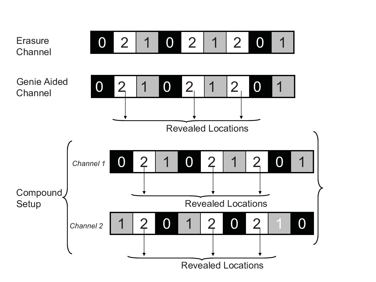
Fig. 1: Main Steps in the Upper Bound (for OPENε=1/3)\varepsilon=1/3). The uppermost figure illustrates the erasure MAC model. Each square corresponds to one channel use. The black squares correspond to 𝘴i=0,{\mathssf{s}}_{i}=0, i.e., 𝘻i=𝘹i⊕𝘺i{\mathssf{z}}_{i}={{\mathssf{x}}}_{i}\oplus{\mathssf{y}}_{i}, the shaded grey squares correspond to 𝘴i=1,{\mathssf{s}}_{i}=1, i.e., 𝘻i=𝘹i{\mathssf{z}}_{i}={{\mathssf{x}}}_{i} and the white squares correspond to 𝘴i=2{\mathssf{s}}_{i}=2 i.e., 𝘻i=𝘺i{\mathssf{z}}_{i}={\mathssf{y}}_{i}. Our upper bound reveals the location of 𝘴i=2{\mathssf{s}}_{i}=2 to both the transmitters non-causally. Since the transmitters are not aware of the location of the grey and black squares, any code for this genie-aided channel must also be decodable when the black and grey squares are interchanged. This compound setup results in a tighter upper bound than the usual cut-set bound.
Theorem 1.

The modulo-sum capacity is upper bounded by the following expression:

C≤R+=(1−3​ε)++(2−ε)3C\leq R^{+}=\frac{(1-3\varepsilon)^{+}+(2-\varepsilon)}{3} (3)

where (⋅)+(\cdot)^{+} equals zero if the argument inside is negative.

The proposed upper bound is tighter than a genie-aided bound where one of the messages, say 𝘸1{\mathssf{w}}_{1}, is revealed to the decoder. We provide the key-steps in the upper bound derivation below.

III-B1 Revealing Side Information to the Transmitters

Our key step is to reveal part of the state sequence to the encoders. In particular define the sets 𝒜={i:𝘴i=1}{\mathcal{A}}=\{i:{\mathssf{s}}_{i}=1\}, ℬ={i:𝘴i=2}{\mathcal{B}}=\{i:{\mathssf{s}}_{i}=2\} and 𝒞={i:𝘴i=0}{\mathcal{C}}=\{i:{\mathssf{s}}_{i}=0\}. We illustrate the technique when |𝒜|=|ℬ|=|𝒞|=n3|{\mathcal{A}}|=|{\mathcal{B}}|=|{\mathcal{C}}|=\frac{n}{3}, which roughly corresponds to the case when ε=1/3\varepsilon=1/3. We will use the notation 𝘻𝒞n{\mathssf{z}}_{{\mathcal{C}}}^{n} to denote the projection of 𝘻n{\mathssf{z}}^{n} onto the indices i∈𝒞i\in{\mathcal{C}} etc.

In our upper bound, we first reveal the knowledge of ℬ{\mathcal{B}} to the two encoders non-causally. However the encoders are not aware of the sets 𝒜{\mathcal{A}} and 𝒞{\mathcal{C}}. Note from (1) that 𝘻ℬn=𝘺ℬn{\mathssf{z}}_{{\mathcal{B}}}^{n}={\mathssf{y}}_{{\mathcal{B}}}^{n}, 𝘻𝒜n=𝘹𝒜n{\mathssf{z}}_{{\mathcal{A}}}^{n}={{\mathssf{x}}}_{{\mathcal{A}}}^{n} and 𝘻𝒞n=𝘹𝒞n⊕𝘺𝒞n{\mathssf{z}}^{n}_{\mathcal{C}}={{\mathssf{x}}}^{n}_{\mathcal{C}}\oplus{\mathssf{y}}^{n}_{\mathcal{C}}.

III-B2 Independence of Input Signals from 𝘸1⊕𝘸2{\mathssf{w}}_{1}\oplus{\mathssf{w}}_{2}

Observe that 𝘺ℬn{\mathssf{y}}_{{\mathcal{B}}}^{n} is sub-sequence transmitted by user 2 and hence independent of 𝘶=𝘸1⊕𝘸2{\mathssf{u}}={\mathssf{w}}_{1}\oplus{\mathssf{w}}_{2}. Using this property we have:

n​R\displaystyle nR =H⁡(𝘶)\displaystyle=H({\mathssf{u}}) (4)
=H⁡(𝘶|𝘺ℬn)\displaystyle=H({\mathssf{u}}|{\mathssf{y}}_{\mathcal{B}}^{n}) (5)
=H⁡(𝘶|𝘺ℬn,𝘹𝒜n,𝘻𝒞n)+I⁡(𝘹𝒜n,𝘻𝒞n;𝘶|𝘺ℬn)\displaystyle=H({\mathssf{u}}|{\mathssf{y}}_{\mathcal{B}}^{n},{{\mathssf{x}}}_{\mathcal{A}}^{n},{\mathssf{z}}_{\mathcal{C}}^{n})+I({{\mathssf{x}}}_{\mathcal{A}}^{n},{\mathssf{z}}_{\mathcal{C}}^{n};{\mathssf{u}}|{\mathssf{y}}_{{\mathcal{B}}}^{n}) (6)
≤n(1−ε)−H(𝘹𝒜n,𝘻𝒞n|𝘺ℬn,𝘶)+n⋅on(1),\displaystyle\leq n(1-\varepsilon)-H({{\mathssf{x}}}_{\mathcal{A}}^{n},{\mathssf{z}}_{{\mathcal{C}}}^{n}|{\mathssf{y}}_{{\mathcal{B}}}^{n},{\mathssf{u}})+n\cdot o_{n}(1), (7)

where we use Fano’s inequality in 1n​H​(𝘶|𝘹𝒜n,𝘺ℬn,𝘻𝒞n)≤on​(1){\frac{1}{n}H({\mathssf{u}}|{{\mathssf{x}}}_{\mathcal{A}}^{n},{\mathssf{y}}_{\mathcal{B}}^{n},{\mathssf{z}}_{\mathcal{C}}^{n})\leq o_{n}(1)} and on​(1)o_{n}(1) denotes a vanishing function in nn.

III-B3 Compound MAC Channel

Observe that the same coding scheme must also work when the positions of sets 𝒜{\mathcal{A}} and 𝒞{\mathcal{C}} are interchanged. This results in

nR≤n(1−ε)−H(𝘹𝒞n,𝘻𝒜n|𝘺ℬn,𝘶)+n⋅on(1).\displaystyle nR\leq n(1-\varepsilon)-H({{\mathssf{x}}}_{\mathcal{C}}^{n},{\mathssf{z}}_{{\mathcal{A}}}^{n}|{\mathssf{y}}_{{\mathcal{B}}}^{n},{\mathssf{u}})+n\cdot o_{n}(1). (8)

Combining (7) and (8) and ignoring the on​(1)o_{n}(1) term, we obtain the following:

nR≤n(1−ε)−max(H(𝘹𝒜n,𝘻𝒞n|𝘺ℬn,𝘶),H(𝘹𝒞n,𝘻𝒜n|𝘺ℬn,𝘶))\displaystyle nR\leq n(1-\varepsilon)-\max\bigg(H({{\mathssf{x}}}_{\mathcal{A}}^{n},{\mathssf{z}}_{{\mathcal{C}}}^{n}|{\mathssf{y}}_{{\mathcal{B}}}^{n},{\mathssf{u}}),H({{\mathssf{x}}}_{\mathcal{C}}^{n},{\mathssf{z}}_{{\mathcal{A}}}^{n}|{\mathssf{y}}_{{\mathcal{B}}}^{n},{\mathssf{u}})\bigg) (9)
≤n(1−ε)−12(H(𝘹𝒜n,𝘻𝒞n|𝘺ℬn,𝘶)+H(𝘹𝒞n,𝘻𝒜n|𝘺ℬn,𝘶))\displaystyle\leq n(1-\varepsilon)-\frac{1}{2}\bigg(H({{\mathssf{x}}}_{\mathcal{A}}^{n},{\mathssf{z}}_{{\mathcal{C}}}^{n}|{\mathssf{y}}_{{\mathcal{B}}}^{n},{\mathssf{u}})\!+\!H({{\mathssf{x}}}_{\mathcal{C}}^{n},{\mathssf{z}}_{{\mathcal{A}}}^{n}|{\mathssf{y}}_{{\mathcal{B}}}^{n},{\mathssf{u}})\bigg) (10)
≤n(1−ε)−12H(𝘹𝒜n,𝘻𝒞n,𝘹𝒞n,𝘻𝒜n|𝘺ℬn,𝘶)\displaystyle\leq n(1-\varepsilon)-\frac{1}{2}H({{\mathssf{x}}}_{\mathcal{A}}^{n},{\mathssf{z}}_{{\mathcal{C}}}^{n},{{\mathssf{x}}}_{\mathcal{C}}^{n},{\mathssf{z}}_{{\mathcal{A}}}^{n}|{\mathssf{y}}_{{\mathcal{B}}}^{n},{\mathssf{u}}) (11)
=n(1−ε)−12H(𝘹𝒜n,𝘺𝒞n,𝘹𝒞n,𝘺𝒜n|𝘺ℬn,𝘶)\displaystyle=n(1-\varepsilon)-\frac{1}{2}H({{\mathssf{x}}}_{\mathcal{A}}^{n},{\mathssf{y}}_{{\mathcal{C}}}^{n},{{\mathssf{x}}}_{\mathcal{C}}^{n},{\mathssf{y}}_{{\mathcal{A}}}^{n}|{\mathssf{y}}_{{\mathcal{B}}}^{n},{\mathssf{u}}) (12)
≤n(1−ε)−12H(𝘺𝒜n,𝘺𝒞n|𝘺ℬn,𝘶)\displaystyle\leq n(1-\varepsilon)-\frac{1}{2}H({\mathssf{y}}_{{\mathcal{A}}}^{n},{\mathssf{y}}_{{\mathcal{C}}}^{n}|{\mathssf{y}}_{{\mathcal{B}}}^{n},{\mathssf{u}}) (13)
≤n⁡(1−ε)−12​H​(𝘺𝒜n,𝘺𝒞n|𝘺ℬn)\displaystyle\leq n(1-\varepsilon)-\frac{1}{2}H({\mathssf{y}}_{{\mathcal{A}}}^{n},{\mathssf{y}}_{{\mathcal{C}}}^{n}|{\mathssf{y}}_{{\mathcal{B}}}^{n}) (14)

where (14) follows from the fact that the transmit sequence by user 22, 𝘺n{\mathssf{y}}^{n} is independent of 𝘸1{\mathssf{w}}_{1} and hence 𝘸1⊕𝘸2{\mathssf{w}}_{1}\oplus{\mathssf{w}}_{2}. Eq. (14) suggests that for the rate to be high (𝘺𝒜n,𝘺𝒞n)({\mathssf{y}}_{{\mathcal{A}}}^{n},{\mathssf{y}}_{{\mathcal{C}}}^{n}) and 𝘺ℬn{\mathssf{y}}_{{\mathcal{B}}}^{n} must be strongly correlated. However as we show below, such a constraint can only reduce the upper bound obtained by revealing one of the messages to the destination.

III-B4 Penalty from Repetition Coding

Suppose that the sequence 𝘹n{{\mathssf{x}}}^{n} is completely revealed to the destination. The receiver only needs to compute 𝘸2{\mathssf{w}}_{2} and hence we have:

n​R\displaystyle nR ≤H⁡(𝘺n)=H⁡(𝘺𝒜n,𝘺𝒞n|𝘺ℬn)+H⁡(𝘺ℬn)\displaystyle\leq H({\mathssf{y}}^{n})=H({\mathssf{y}}_{\mathcal{A}}^{n},{\mathssf{y}}_{\mathcal{C}}^{n}|{\mathssf{y}}_{\mathcal{B}}^{n})+H({\mathssf{y}}_{{\mathcal{B}}}^{n}) (15)

Eliminating the joint entropy term between (14) and (15) we get

32​n​R\displaystyle\frac{3}{2}nR ≤12​H​(𝘺ℬn)+n⁡(1−ε)\displaystyle\leq\frac{1}{2}H({\mathssf{y}}_{{\mathcal{B}}}^{n})+n(1-\varepsilon) (16)

By using the simple upper bound H⁡(𝘺ℬn)≤|ℬ|=n​εH({\mathssf{y}}_{\mathcal{B}}^{n})\leq|{\mathcal{B}}|=n\varepsilon we get R≤2−ε3R\leq\frac{2-\varepsilon}{3} which agrees with (3) for ε=1/3\varepsilon=1/3.

III-C Causal State Feedback

Consider the case when the encoders are revealed the state sequences in a strictly causal manner. The encoding functions at time ii can depend on the state sequence up to time i−1i-1 i.e. 𝘹i=fi​(𝘸1,𝘴1i−1){{\mathssf{x}}}_{i}=f_{i}({\mathssf{w}}_{1},{\mathssf{s}}_{1}^{i-1}) and 𝘺i=gi​(𝘸2,𝘴1i−1){\mathssf{y}}_{i}=g_{i}({\mathssf{w}}_{2},{\mathssf{s}}_{1}^{i-1}).

Proposition 2.

The modulo-sum capacity the multiple access channel with strictly causal state feedback is lower and upper bounded by RFB−≤C≤RFB+R_{\mathrm{FB}}^{-}\leq C\leq R_{\mathrm{FB}}^{+}, where

RFB−\displaystyle R_{\mathrm{FB}}^{-} =11+2​ε.\displaystyle=\frac{1}{1+2\varepsilon}. (17)
RFB+\displaystyle R_{\mathrm{FB}}^{+} =1−ε\displaystyle=1-\varepsilon (18)

The lower bound is achieved by a two-phase protocol where the users transmit uncoded bits in the first phase and use a multiple-access code in the second phase. The upper bound is the genie-aided bound where one of the messages is revealed to the destination. The problem reduces to communicating the other message, say 𝘸2{\mathssf{w}}_{2} to the destination. Feedback in such a case is well known to not increase the point-to-point capacity.

III-D Numerical Comparisons

Refer to caption
Fig. 2: Comparison of upper and lower bounds for the Erasure-MAC channel with and without feedback.

Fig. 2 provides a numerical computation of the upper and lower bounds for the Erasure MAC channel both with and without feedback. The upper-most dotted curve corresponds to RFB+=1−εR^{+}_{\mathrm{FB}}=1-\varepsilon and is the upper bound on the capacity with feedback. The lowermost curve, marked with backward arrows, is the lower bound achieved by either the decode and forward or the compute and forward schemes. The other solid curve is our new upper bound on the capacity without feedback (c.f. Theorem 1). The fourth curve is the lower bound with feedback in Prop. 2. Interestingly we see that it lies above the upper bound for certain values of ε\varepsilon, thus establishing that feedback helps in computation over the erasure multiple access channel.

III-E Lossy Reconstruction

While the focus of this paper is on lossless recovery, our ideas can be also extended to lossy recovery. We illustrate this with one example. As before we consider the case when the two transmitters observe i.i.d. equiprobable binary sequences 𝘣1k{\mathssf{b}}_{1}^{k} and 𝘣2k{\mathssf{b}}_{2}^{k} respectively. The receiver is interested in the modulo-sum 𝘶k=𝘣1k⊕𝘣2k{\mathssf{u}}^{k}={\mathssf{b}}_{1}^{k}\oplus{\mathssf{b}}_{2}^{k}. However it suffices to output any sequence 𝘶^k\hat{{\mathssf{u}}}^{k} that satisfies the distortion constraint

E⁡[1k​∑i=1kρ⁡(𝘶i,𝘶^i)]≤D\displaystyle E\left[\frac{1}{k}\sum_{i=1}^{k}\rho({\mathssf{u}}_{i},\hat{{\mathssf{u}}}_{i})\right]\leq D (19)

where ρ⁡(⋅,⋅)\rho(\cdot,\cdot) is the associated distortion measure. In this paper we select the erasure distortion measure i.e.,

ρ⁡(𝘶,𝘶^)={0,𝘶^=𝘶1,𝘶^=⋆∞, otherwise\displaystyle\rho({\mathssf{u}},\hat{{\mathssf{u}}})=\begin{cases}0,&\hat{{\mathssf{u}}}={\mathssf{u}}\\ 1,&\hat{{\mathssf{u}}}=\star\\ \infty,&\text{ otherwise}\end{cases} (20)

We assume a bandwidth expansion factor of β\beta. Thus the number of channel uses is n=k​βn=k\beta and the transmitters generate 𝘹in=fk​(𝘣ik){{\mathssf{x}}}_{i}^{n}=f_{k}({\mathssf{b}}_{i}^{k}) for i=1,2i=1,2 and the receiver outputs 𝘶^k=gk​(𝘻n,𝘴n)\hat{{\mathssf{u}}}^{k}=g_{k}({\mathssf{z}}^{n},{\mathssf{s}}^{n}). A distortion DD is achievable if there exist a sequence of encoding and decoding functions that satisfy (19) as k→∞k\rightarrow\infty. We develop bounds on the achievable distortion.

Theorem 2.

An achievable distortion for modulo-sum reconstruction of equiprobable and independent binary sources over the erasure multiple access channel satisfies Douter≤D≤DinnerD_{\mathrm{outer}}\leq D\leq D_{\mathrm{inner}} where

Dinner\displaystyle D_{\mathrm{inner}} =(1−β​R−)+\displaystyle=(1-\beta R^{-})^{+} (21)
Douter\displaystyle D_{\mathrm{outer}} =(1−β​R+)+\displaystyle=\left(1-\beta R^{+}\right)^{+} (22)

where R−R^{-} and R+R^{+} are the lower and upper bounds on the modulo-sum capacity stated in (2) and (3) respectively and the function (v)+(v)^{+} equals zero if v<0v<0 and equals vv otherwise.

In particular, examining the expression for DinnerD_{\mathrm{inner}} it can be shown that uncoded transmission is sub-optimal even when β=1\beta=1 i.e., there is no bandwidth mis-match. If the two users select 𝘹in=𝘴in{{\mathssf{x}}}_{i}^{n}={\mathssf{s}}_{i}^{n} for i=1,2i=1,2 then the destination must declare an erasure whenever 𝘴i≠0{\mathssf{s}}_{i}\neq 0. It is easy to see that the average distortion for this technique equals 2​ε2\varepsilon. In contrast the expression (21) equals min⁡(2​ε,12)\min(2\varepsilon,\frac{1}{2}) when β=1\beta=1. This is a strict improvement for ε∈(14,12)\varepsilon\in\left(\frac{1}{4},\frac{1}{2}\right).

III-F Extended Multiple Access Channel

We consider an extension of the model in (1) where when there are two additional states — either the decoder observes both (𝘹,𝘺)({{\mathssf{x}}},{\mathssf{y}}) or it observes an erasure. In particular we have that, 𝘴∈{0,1,2,3,4},{\mathssf{s}}\in\{0,1,2,3,4\}, where

𝘻={𝘹⊕𝘺,𝘴=0,𝘹,𝘴=1,𝘺,𝘴=2,(𝘹,𝘺),𝘴=3,⋆,𝘴=4.\displaystyle{\mathssf{z}}=\begin{cases}{{\mathssf{x}}}\oplus{\mathssf{y}},&{\mathssf{s}}=0,\\ {{\mathssf{x}}},&{\mathssf{s}}=1,\\ {\mathssf{y}},&{\mathssf{s}}=2,\\ ({{\mathssf{x}}},{\mathssf{y}}),&{\mathssf{s}}=3,\\ \star,&{\mathssf{s}}=4.\end{cases} (23)

Our upper and lower bounds can be naturally extended to the extended multiple access channel (23). For simplicity we only focus on the lossless case. Let Pr⁡(𝘴=1)=Pr⁡(𝘴=2)=δ⋅ε\Pr({\mathssf{s}}=1)=\Pr({\mathssf{s}}=2)=\delta\cdot\varepsilon, Pr⁡(𝘴=0)=δ⁡(1−2​ε)\Pr({\mathssf{s}}=0)=\delta(1-2\varepsilon), Pr⁡(𝘴=3)=γ\Pr({\mathssf{s}}=3)=\gamma and Pr⁡(𝘴=4)=1−γ−δ\Pr({\mathssf{s}}=4)=1-\gamma-\delta.

Proposition 3.

The modulo-sum capacity of the extended multiple access channel in (23) satisfies R−≤C≤R+R^{-}\leq C\leq R^{+}, where:

R−\displaystyle R^{-} =γ+δ⋅max⁡(12,(1−2​ε))\displaystyle=\gamma+\delta\cdot\max\left(\frac{1}{2},(1-2\varepsilon)\right) (24)
R+\displaystyle R^{+} =γ+δ⁡(2−ε+(1−3​ε)+3)\displaystyle=\gamma+\delta\left(\frac{2-\varepsilon+(1-3\varepsilon)^{+}}{3}\right) (25)

We observe that the lower and upper bounds for the extended model reduce to the corresponding bounds for the simplified model when γ=0\gamma=0 and δ=1\delta=1.

IV Lower Bound: Proof of Prop. 1

We separately establish the achievability of R=1−2​εR=1-2\varepsilon and R=1/2R=1/2.

IV-A Compute and Forward Scheme

We use identical linear codebooks at the two transmitters in the compute and forward scheme to achieve R=1−2​ε{R=1-2\varepsilon}. Recall that the messages 𝐰1{\mathbf{w}}_{1} and 𝐰2{\mathbf{w}}_{2} are assumed to be binary valued sequences of length n​RnR bits i.e., we take

𝐛iT=[bi​1,…,bi​K]{\mathbf{b}}_{i}^{T}=\left[b_{i1},\ldots,b_{iK}\right] (26)

where K=n​RK=nR denote the number of information bits in the message. Let GG be a matrix of dimensions K×nK\times n, and let each entry in GG be sampled independently from an equiprobable Bernoulli distribution. It is useful to express

𝐆=[𝐠1,…,𝐠n]{\mathbf{G}}=\left[{\mathbf{g}}_{1},\ldots,{\mathbf{g}}_{n}\right] (27)

where each 𝐠i∈{0,1}K{\mathbf{g}}_{i}\in\{0,1\}^{K} is a length KK binary valued column vector. The transmitted sequence 𝐱T=[x1,…,xK]{\mathbf{x}}^{T}=[x_{1},\ldots,x_{K}] at receiver 11 is expressed as:

𝐱T\displaystyle{\mathbf{x}}^{T} =𝐛1T⋅G\displaystyle={\mathbf{b}}_{1}^{T}\cdot G (28)
=[𝐛1T​𝐠1,…,𝐛1T​𝐠n]\displaystyle=[{\mathbf{b}}_{1}^{T}{\mathbf{g}}_{1},\ldots,{\mathbf{b}}_{1}^{T}{\mathbf{g}}_{n}] (29)

The transmitted sequence 𝐲T{\mathbf{y}}^{T} at user 22 is defined in a similar manner.

The receiver is interested in computing

𝐮T=𝐛1T⊕𝐛2T=[b11⊕b21,…,b1​K⊕b2​K].\displaystyle{\mathbf{u}}^{T}={\mathbf{b}}_{1}^{T}\oplus{\mathbf{b}}_{2}^{T}=\left[b_{11}\oplus b_{21},\ldots,b_{1K}\oplus b_{2K}\right]. (30)

Given our specific encoder, the received symbol can be expressed as:

𝘻i={(𝐛1T⊕𝐛2T)​𝐠i,𝘴i=0,𝐛1T​𝐠i,𝘴i=1,𝐛2T​𝐠i,𝘴i=2.\displaystyle{\mathssf{z}}_{i}=\begin{cases}({\mathbf{b}}_{1}^{T}\oplus{\mathbf{b}}_{2}^{T}){\mathbf{g}}_{i},&{\mathssf{s}}_{i}=0,\\ {\mathbf{b}}_{1}^{T}{\mathbf{g}}_{i},&{\mathssf{s}}_{i}=1,\\ {\mathbf{b}}_{2}^{T}{\mathbf{g}}_{i},&{\mathssf{s}}_{i}=2.\end{cases} (31)

Our proposed decoder only uses the output of the channel when 𝘴i=0{\mathssf{s}}_{i}=0 and declares erasures if 𝘴i≠0{\mathssf{s}}_{i}\neq 0. Let G^0=G|𝘴i=0\hat{G}_{0}=G_{|{\mathssf{s}}_{i}=0} be collection of column vectors in GG when 𝘴i=0{\mathssf{s}}_{i}=0. We use the following lemma regarding G^0\hat{G}_{0}:

Lemma 1.

For every δ>0\delta>0, there exists a function on,δ​(1)o_{n,\delta}(1) that goes to zero as n→∞n\rightarrow\infty, such that following holds:

Pr⁡(rank⁡(G^0)≥min⁡(K,n⁡(1−2​ε−δ)))≥1−on,δ​(1).\displaystyle\Pr\left(\mathrm{rank}(\hat{G}_{0})\geq\min(K,n(1-2\varepsilon-\delta))\right)\geq 1-o_{n,\delta}(1). (32)

The proof of Lemma 1 is obtained by showing that, with high probability, each randomly selected column of G^0\hat{G}_{0} is in a general position. We omit the proof. Clearly the receiver can uniquely recover (𝐛1T⊕𝐛2T)({\mathbf{b}}_{1}^{T}\oplus{\mathbf{b}}_{2}^{T}) from

𝐳0T=(𝐛1T⊕𝐛2T)⋅G^0\displaystyle{\mathbf{z}}_{0}^{T}=({\mathbf{b}}_{1}^{T}\oplus{\mathbf{b}}_{2}^{T})\cdot\hat{G}_{0} (33)

if G^0\hat{G}_{0} has full row-rank, which holds if R≤1−2​ε−δR\leq 1-2\varepsilon-\delta. Since δ>0\delta>0 is arbitrary this establishes our first lower bound.

IV-B Achievability of R=1/2R=1/2: Decode and Forward Approach

The rate R=1/2R=1/2 is achieved by transmitting both 𝘸1{\mathssf{w}}_{1} and 𝘸2{\mathssf{w}}_{2} to the destination instead of taking advantage of the fact that the destination only requires 𝘸1⊕𝘸2{\mathssf{w}}_{1}\oplus{\mathssf{w}}_{2}. The multiple access capacity region is given by the convex hull of rate pairs (R1,R2)(R_{1},R_{2}) that satisfy:

R1\displaystyle R_{1} ≤I⁡(𝘹;𝘻,𝘴|𝘺)\displaystyle\leq I({{\mathssf{x}}};{\mathssf{z}},{\mathssf{s}}|{\mathssf{y}}) (34)
R2\displaystyle R_{2} ≤I⁡(𝘺;𝘻,𝘴|𝘹)\displaystyle\leq I({\mathssf{y}};{\mathssf{z}},{\mathssf{s}}|{{\mathssf{x}}}) (35)
R1+R2\displaystyle R_{1}+R_{2} ≤I⁡(𝘹,𝘺,𝘻,𝘴)\displaystyle\leq I({{\mathssf{x}}},{\mathssf{y}};{\mathssf{z}},{\mathssf{s}}) (36)

Taking 𝘹{{\mathssf{x}}} and 𝘺{\mathssf{y}} to be independent equiprobable binary symbols we get that MAC Capacity region contains R1≤1−εR_{1}\leq 1-\varepsilon, R2≤1−εR_{2}\leq 1-\varepsilon and R1+R2≤1R_{1}+R_{2}\leq 1. Since ε<1/2\varepsilon<1/2 the rate pair R1=R2=12R_{1}=R_{2}=\frac{1}{2} is achievable. Thus each user can transmit 𝘸i{\mathssf{w}}_{i} at a rate of R=1/2R=1/2 to the destination. The destination then computes 𝘸1⊕𝘸2{\mathssf{w}}_{1}\oplus{\mathssf{w}}_{2}.

Remark 1.

The rate R=1/2R=1/2 can be achieved using a decode and forward scheme even when the two transmitters use identical codebooks. As established in [11], in addition to (34)-(36), an additional constraint

R≤I⁡(𝘹,𝘺;𝘻,𝘴|𝘹⊕𝘺)=2​εR\leq I({{\mathssf{x}}},{\mathssf{y}};{\mathssf{z}},{\mathssf{s}}|{{\mathssf{x}}}\oplus{\mathssf{y}})=2\varepsilon

must be satisfied when identical codebooks are used. Thus the achievable rate now reduces to R=min⁡(1/2,2​ε)R=\min(1/2,2\varepsilon). Note that with with identical codebooks, the rate R=1/2R=1/2 is achievable for ε>1/4\varepsilon>1/4, the region in which decode and forward dominates compute and forward discussed before.

IV-C Achieving R=1/2R=1/2 with Compute and Forward

The rate R=1/2R=1/2 can also be achieved using identical linear codes if the receiver does not ignore the output when 𝘴i≠0{\mathssf{s}}_{i}\neq 0. Let Let G^0=G|𝘴i=0\hat{G}_{0}=G_{|{\mathssf{s}}_{i}=0}, G^1=G|𝘴i=1\hat{G}_{1}=G_{|{\mathssf{s}}_{i}=1} and G^2=G|𝘴i=2\hat{G}_{2}=G_{|{\mathssf{s}}_{i}=2} be the projections of GG onto the indices where 𝘴i=0{\mathssf{s}}_{i}=0, 𝘴i=1{\mathssf{s}}_{i}=1 and 𝘴i=2{\mathssf{s}}_{i}=2 respectively. Following (31), we let 𝐳𝒞T=(𝐛1T+𝐛2T)​G^0{\mathbf{z}}_{\mathcal{C}}^{T}=({\mathbf{b}}_{1}^{T}+{\mathbf{b}}_{2}^{T})\hat{G}_{0}, 𝐳𝒜T=𝐛1T​G^1{\mathbf{z}}_{\mathcal{A}}^{T}={\mathbf{b}}_{1}^{T}\hat{G}_{1} and 𝐳ℬT=𝐛2T​G^2{\mathbf{z}}_{\mathcal{B}}^{T}={\mathbf{b}}_{2}^{T}\hat{G}_{2}. Furthermore along the lines of Lemma 1, it follows that for any δ>0\delta>0, with a probability that exceeds 1−on,δ​(1)1-o_{n,\delta}(1), we have that

dim⁡(col​-​space​(G^1)∪col​-​space​(G^2))\displaystyle\mathrm{dim}\left(\mathrm{col\text{-}space}({\hat{G}_{1}})\cup\mathrm{col\text{-}space}({\hat{G}_{2}})\right) ≤n⋅min⁡(2​ε+δ,R)\displaystyle\leq n\cdot\min(2\varepsilon+\delta,R) (37)

and since the columns of G^i{\hat{G}_{i}} are independently sampled, it follows that,

dim⁡(col​-​space​(G^i))\displaystyle\mathrm{dim}\left(\mathrm{col\text{-}space}({\hat{G}_{i}})\right) ≥n⋅min(ε−δ2,R),i=1,2.\displaystyle\geq n\cdot\min(\varepsilon-\frac{\delta}{2},R),\quad i=1,2. (38)

Thus using the relation

dim⁡(col​-​space​(G^1)∩col​-​space​(G^2))=dim⁡(col​-​space​(G^1))\displaystyle\mathrm{dim}\left(\mathrm{col\text{-}space}({\hat{G}_{1}})\cap\mathrm{col\text{-}space}({\hat{G}_{2}})\right)\!\!=\mathrm{dim}\left(\mathrm{col\text{-}space}({\hat{G}_{1}})\right)
+dim⁡(col​-​space​(G^2))−dim⁡(col​-​space​(G^1)∪col​-​space​(G^2))\displaystyle\!\!+\!\!\mathrm{dim}\left(\mathrm{col\text{-}space}({\hat{G}_{2}})\right)\!\!-\!\!\mathrm{dim}\left(\mathrm{col\text{-}space}({\hat{G}_{1}})\cup\mathrm{col\text{-}space}({\hat{G}_{2}})\right) (39)

it follows that with a probability that exceeds 1−on,δ​(1)1-o_{n,\delta}(1), we have that

dim⁡(col​-​space​(G^1)∩col​-​space​(G^2))\displaystyle\mathrm{dim}\left(\mathrm{col\text{-}space}({\hat{G}_{1}})\cap\mathrm{col\text{-}space}({\hat{G}_{2}})\right) ≥n⋅d12\displaystyle\geq n\cdot d_{12}
=Δn​(2​ε−R−δ)+\displaystyle\stackrel{{\scriptstyle\Delta}}{{=}}n\left(2\varepsilon-R-\delta\right)^{+} (40)

Thus one can find a matrices MiM_{i} such that

G^1​M1=G^2​M2=A\hat{G}_{1}M_{1}=\hat{G}_{2}M_{2}=A (41)

where AA is a full-matrix of dimension n×d12n\times d_{12}. The receiver first computes

(𝐳𝒜T⊕𝐳ℬT)​M\displaystyle({\mathbf{z}}_{\mathcal{A}}^{T}\oplus{\mathbf{z}}_{\mathcal{B}}^{T})M =(𝐛1T⊕𝐛2T)⋅A\displaystyle=({\mathbf{b}}_{1}^{T}\oplus{\mathbf{b}}_{2}^{T})\cdot A (42)

and then needs to compute 𝐛1⊕𝐛2{\mathbf{b}}_{1}\oplus{\mathbf{b}}_{2} from (𝐛1⊕𝐛2)T​[G^0​A]({\mathbf{b}}_{1}\oplus{\mathbf{b}}_{2})^{T}[\hat{G}_{0}~~A]. Since the entries in G^0\hat{G}_{0} and AA are independent the rank of [G^0​A][\hat{G}_{0}~~A] is, with high probability at-least n⁡(d12+1−2​ε−δ)n(d_{12}+1-2\varepsilon-\delta). From (40) we can show that R=max⁡(12,1−2​ε)R=\max(\frac{1}{2},1-2\varepsilon) is achievable.

V Upper Bound: Proof of Theorem 1

We begin with some notation. For a given sequence sns^{n} 𝒜⁡(sn)={i:si=1}{\mathcal{A}}(s^{n})=\{i:s_{i}=1\} and ℬ⁡(sn)={i:si=2}{\mathcal{B}}(s^{n})=\{i:s_{i}=2\}. Let 𝒞⁡(sn)={i:si=0}{\mathcal{C}}(s^{n})=\{i:s_{i}=0\}. Define 𝘹𝒜⁡(sn)n{{\mathssf{x}}}^{n}_{{\mathcal{A}}(s^{n})} to be the projection of the sequence 𝘹n{{\mathssf{x}}}^{n} on the indices where si=1s_{i}=1 and use a similar notation for other indices.

Since the receiver decodes 𝘶=𝘸1⊕𝘸2{\mathssf{u}}={\mathssf{w}}_{1}\oplus{\mathssf{w}}_{2} from its output, from Fano’s inequality, we have that

1n​H​(𝘶|𝘴n,𝘻n)≤δn\displaystyle\frac{1}{n}H\left({\mathssf{u}}~|~{\mathssf{s}}^{n},{\mathssf{z}}^{n}\right)\leq\delta_{n} (43)

for some sequence δn\delta_{n} that goes to zero as n→∞n\rightarrow\infty.

Now consider

n​R\displaystyle nR =H⁡(𝘶)\displaystyle=H({\mathssf{u}}) (44)
=H⁡(𝘶|𝘴n)\displaystyle=H({\mathssf{u}}|{\mathssf{s}}^{n}) (45)
=H⁡(𝘶|𝘴n,𝘺ℬ⁡(𝘴n)n)\displaystyle=H({\mathssf{u}}|{\mathssf{s}}^{n},{\mathssf{y}}^{n}_{{\mathcal{B}}({\mathssf{s}}^{n})}) (46)
=nδn+I(𝘶;𝘹𝒜⁡(𝘴n)n,𝘻𝒞⁡(𝘴n)n|𝘴n,𝘺ℬ⁡(𝘴n)n)\displaystyle=n\delta_{n}+I({\mathssf{u}};{{\mathssf{x}}}_{{\mathcal{A}}({\mathssf{s}}^{n})}^{n},{\mathssf{z}}^{n}_{{\mathcal{C}}({\mathssf{s}}^{n})}|{\mathssf{s}}^{n},{\mathssf{y}}^{n}_{{\mathcal{B}}({\mathssf{s}}^{n})}) (47)
=nδn+H(𝘹𝒜⁡(𝘴n)n,𝘻𝒞⁡(𝘴n)n|𝘴n,𝘺ℬ⁡(𝘴n)n)\displaystyle=n\delta_{n}+H({{\mathssf{x}}}_{{\mathcal{A}}({\mathssf{s}}^{n})}^{n},{\mathssf{z}}^{n}_{{\mathcal{C}}({\mathssf{s}}^{n})}|{\mathssf{s}}^{n},{\mathssf{y}}^{n}_{{\mathcal{B}}({\mathssf{s}}^{n})})
−H(𝘹𝒜⁡(𝘴n)n,𝘻𝒞⁡(𝘴n)n|𝘴n,𝘺ℬ⁡(𝘴n)n,𝘶)\displaystyle\qquad-H({{\mathssf{x}}}_{{\mathcal{A}}({\mathssf{s}}^{n})}^{n},{\mathssf{z}}^{n}_{{\mathcal{C}}({\mathssf{s}}^{n})}|{\mathssf{s}}^{n},{\mathssf{y}}^{n}_{{\mathcal{B}}({\mathssf{s}}^{n})},{\mathssf{u}}) (48)

where (45) follows from the fact that the message 𝘶{\mathssf{u}} is independent of the sequence 𝘴n{\mathssf{s}}^{n}. Eq. (46) follows from the fact that 𝘶=𝘸1⊕𝘸2{\mathssf{u}}={\mathssf{w}}_{1}\oplus{\mathssf{w}}_{2} is independent of 𝘸2{\mathssf{w}}_{2} and hence also independent of 𝘺n{\mathssf{y}}^{n}. Eq. (47) follows from the chain rule of mutual information and the application of Fano’s inequality.

We upper bound the first entropy term in (48) as follows.

H(𝘹𝒜⁡(𝘴n)n,𝘻𝒞⁡(𝘴n)n|𝘴n,𝘺ℬ⁡(𝘴n)n)≤H(𝘹𝒜⁡(𝘴n)n,𝘻𝒞⁡(𝘴n)n|𝘴n),\displaystyle H({{\mathssf{x}}}_{{\mathcal{A}}({\mathssf{s}}^{n})}^{n},{\mathssf{z}}^{n}_{{\mathcal{C}}({\mathssf{s}}^{n})}|{\mathssf{s}}^{n},{\mathssf{y}}^{n}_{{\mathcal{B}}({\mathssf{s}}^{n})})\leq H({{\mathssf{x}}}_{{\mathcal{A}}({\mathssf{s}}^{n})}^{n},{\mathssf{z}}^{n}_{{\mathcal{C}}({\mathssf{s}}^{n})}|{\mathssf{s}}^{n}), (49)
≤∑sn∈𝒮nPr⁡(𝘴n=sn)​(|𝒜⁡(sn)|+|𝒞⁡(sn)|)\displaystyle\leq\sum_{s^{n}\in{\mathcal{S}}^{n}}\Pr({\mathssf{s}}^{n}=s^{n})\left(|{\mathcal{A}}(s^{n})|+|{\mathcal{C}}(s^{n})|\right) (50)
=n⁡(1−ε)+n​δn\displaystyle=n(1-\varepsilon)+n\delta_{n} (51)

where (49) follows from the fact that conditioning reduces entropy. Eq. (50) follows from the fact that both 𝘹n{{\mathssf{x}}}^{n} and 𝘻n{\mathssf{z}}^{n} are binary sequences. Eq. (51) follows from the fact that 𝘴n{\mathssf{s}}^{n} is sampled i.i.d. from a distribution with Pr⁡(𝘴=0)=1−2​ε\Pr({\mathssf{s}}=0)=1-2\varepsilon and Pr⁡(𝘴=1)=Pr⁡(𝘴=2)=ε\Pr({\mathssf{s}}=1)=\Pr({\mathssf{s}}=2)=\varepsilon.

Substituting (51) into (48) we have:

n​R\displaystyle nR ≤n(1−ε)+nδn−H(𝘹𝒜⁡(𝘴n)n,𝘻𝒞⁡(𝘴n)n|𝘴n,𝘺ℬ⁡(𝘴n)n,𝘶)\displaystyle\leq n(1-\varepsilon)+n\delta_{n}-H({{\mathssf{x}}}_{{\mathcal{A}}({\mathssf{s}}^{n})}^{n},{\mathssf{z}}^{n}_{{\mathcal{C}}({\mathssf{s}}^{n})}|{\mathssf{s}}^{n},{\mathssf{y}}^{n}_{{\mathcal{B}}({\mathssf{s}}^{n})},{\mathssf{u}}) (52)

We now separately consider the cases when either 0≤ε<130\leq\varepsilon<\frac{1}{3} and when 13<ε≤12\frac{1}{3}<\varepsilon\leq\frac{1}{2}

V-A Case: 13<ε≤12\frac{1}{3}<\varepsilon\leq\frac{1}{2}

Let 𝒯n⊂𝒮n{\mathcal{T}}_{n}\subset{\mathcal{S}}^{n} be the set of all sequences such that

|𝒜⁡(sn)|>|𝒞⁡(sn)|.|{\mathcal{A}}(s^{n})|>|{\mathcal{C}}(s^{n})|.

By the weak law of large numbers we have that Pr⁡(𝘴n∈𝒯n)≥1−δn\Pr({\mathssf{s}}^{n}\in{\mathcal{T}}_{n})\geq 1-\delta_{n} and Pr⁡(𝘴n∈𝒯n)≤δn\Pr({\mathssf{s}}^{n}\in{\mathcal{T}}_{n})\leq\delta_{n} for some sequence δn\delta_{n} that approaches zero as n→∞n\rightarrow\infty.

For each sn∈𝒯ns^{n}\in{\mathcal{T}}_{n} we define a permutation function as follows. Let 𝒜1​(sn){\mathcal{A}}_{1}(s^{n}) denotes the first |𝒞⁡(sn)||{\mathcal{C}}(s^{n})| indices of sns^{n} where si=1s_{i}=1 and 𝒜2​(sn){\mathcal{A}}_{2}(s^{n}) denotes the remaining indices. Thus 𝒜⁡(sn)=𝒜1​(sn)∪𝒜2​(sn){\mathcal{A}}(s^{n})={\mathcal{A}}_{1}(s^{n})\cup{\mathcal{A}}_{2}(s^{n}) and every element in 𝒜1​(sn){\mathcal{A}}_{1}(s^{n}) is smaller than every element of 𝒜2​(sn){\mathcal{A}}_{2}(s^{n}). The permutation function π⁡(sn)\pi(s^{n}) is chosen such that 𝒞⁡(π⁡(sn))=𝒜1​(sn){\mathcal{C}}(\pi(s^{n}))={\mathcal{A}}_{1}(s^{n}) and 𝒜1​(π⁡(sn))=𝒞⁡(sn){\mathcal{A}}_{1}(\pi(s^{n}))={\mathcal{C}}(s^{n}). Furthermore 𝒜2​(π⁡(sn))=𝒜2​(sn){\mathcal{A}}_{2}(\pi(s^{n}))={\mathcal{A}}_{2}(s^{n}) and ℬ⁡(π⁡(sn))=ℬ⁡(sn){\mathcal{B}}(\pi(s^{n}))={\mathcal{B}}(s^{n}). Note that |𝒜⁡(sn)|=|𝒜⁡(π⁡(sn))||{\mathcal{A}}(s^{n})|=|{\mathcal{A}}(\pi(s^{n}))|, |ℬ⁡(sn)|=|ℬ⁡(π⁡(sn))||{\mathcal{B}}(s^{n})|=|{\mathcal{B}}(\pi(s^{n}))| and |𝒞⁡(sn)|=|𝒞⁡(π⁡(sn))||{\mathcal{C}}(s^{n})|=|{\mathcal{C}}(\pi(s^{n}))| holds. Furthermore since the probability of each sequence only depends on its type, we have Pr⁡(𝘴n=sn)=Pr⁡(𝘴n=π⁡(sn))\Pr({\mathssf{s}}^{n}=s^{n})=\Pr({\mathssf{s}}^{n}=\pi(s^{n})) for each sn∈𝒯ns^{n}\in{\mathcal{T}}_{n}.

Observe that for each 𝘴n=sn∈𝒯n{\mathssf{s}}^{n}=s^{n}\in{\mathcal{T}}_{n} we have that,

H(𝘹𝒜⁡(sn)n,𝘻𝒞⁡(sn)n|𝘺ℬ⁡(sn)n,𝘶,𝘴n)\displaystyle\!\!H({{\mathssf{x}}}_{{\mathcal{A}}(s^{n})}^{n},{\mathssf{z}}^{n}_{{\mathcal{C}}(s^{n})}|{\mathssf{y}}^{n}_{{\mathcal{B}}(s^{n})},\!{\mathssf{u}},{\mathssf{s}}^{n})
+H(𝘹𝒜⁡(π⁡(sn))n,𝘻𝒞⁡(π⁡(sn))n|𝘺ℬ⁡(π⁡(sn))n,𝘶,𝘴n)\displaystyle\qquad+\!\!H({{\mathssf{x}}}_{{\mathcal{A}}(\pi(s^{n}))}^{n},{\mathssf{z}}^{n}_{{\mathcal{C}}(\pi(s^{n}))}|{\mathssf{y}}^{n}_{{\mathcal{B}}(\pi(s^{n}))},\!{\mathssf{u}},{\mathssf{s}}^{n}) (53)
=H(𝘹𝒜1​(sn)n,𝘹𝒜2​(sn)n,𝘻𝒞⁡(sn)n|𝘺ℬ⁡(sn)n,𝘶,𝘴n)\displaystyle=H({{\mathssf{x}}}_{{\mathcal{A}}_{1}(s^{n})}^{n},{{\mathssf{x}}}_{{\mathcal{A}}_{2}(s^{n})}^{n},{\mathssf{z}}^{n}_{{\mathcal{C}}(s^{n})}|{\mathssf{y}}^{n}_{{\mathcal{B}}(s^{n})},\!{\mathssf{u}},{\mathssf{s}}^{n})\!\!
+H(𝘹𝒜1​(π⁡(sn))n,𝘹𝒜2​(π⁡(sn))n,𝘻𝒞⁡(π⁡(sn))n|𝘺ℬ⁡(π⁡(sn))n,𝘶,𝘴n)\displaystyle\qquad+H({{\mathssf{x}}}_{{\mathcal{A}}_{1}(\pi(s^{n}))}^{n},{{\mathssf{x}}}_{{\mathcal{A}}_{2}(\pi(s^{n}))}^{n},{\mathssf{z}}^{n}_{{\mathcal{C}}(\pi(s^{n}))}|{\mathssf{y}}^{n}_{{\mathcal{B}}(\pi(s^{n}))},\!{\mathssf{u}},{\mathssf{s}}^{n}) (54)
=H(𝘹𝒜1​(sn)n,𝘹𝒜2​(sn)n,𝘻𝒞⁡(sn)n|𝘺ℬ⁡(sn)n,𝘶,𝘴n)\displaystyle=H({{\mathssf{x}}}_{{\mathcal{A}}_{1}(s^{n})}^{n},{{\mathssf{x}}}_{{\mathcal{A}}_{2}(s^{n})}^{n},{\mathssf{z}}^{n}_{{\mathcal{C}}(s^{n})}|{\mathssf{y}}^{n}_{{\mathcal{B}}(s^{n})},\!{\mathssf{u}},{\mathssf{s}}^{n})\!\!
+H(𝘹𝒞⁡(sn)n,𝘹𝒜2​(sn)n,𝘻𝒜1​(sn)n|𝘺ℬ⁡(sn)n,𝘶,𝘴n)\displaystyle\qquad+H({{\mathssf{x}}}_{{\mathcal{C}}(s^{n})}^{n},{{\mathssf{x}}}_{{\mathcal{A}}_{2}(s^{n})}^{n},{\mathssf{z}}^{n}_{{\mathcal{A}}_{1}(s^{n})}|{\mathssf{y}}^{n}_{{\mathcal{B}}(s^{n})},\!{\mathssf{u}},{\mathssf{s}}^{n}) (55)
≥H(𝘹𝒜1​(sn)n,𝘹𝒜2​(sn)n,𝘻𝒞⁡(sn)n,𝘹𝒞⁡(sn)n,𝘻𝒜1​(sn)n|𝘺ℬ⁡(sn)n𝘶,𝘴n)\displaystyle\geq H({{\mathssf{x}}}_{{\mathcal{A}}_{1}(s^{n})}^{n},{{\mathssf{x}}}_{{\mathcal{A}}_{2}(s^{n})}^{n},{\mathssf{z}}^{n}_{{\mathcal{C}}(s^{n})},{{\mathssf{x}}}_{{\mathcal{C}}(s^{n})}^{n},{\mathssf{z}}^{n}_{{\mathcal{A}}_{1}(s^{n})}|{\mathssf{y}}^{n}_{{\mathcal{B}}(s^{n})}\!{\mathssf{u}},{\mathssf{s}}^{n}) (56)
≥H(𝘺𝒜1​(sn)n,𝘺𝒞⁡(sn)n|𝘺ℬ⁡(sn)n,𝘴n)\displaystyle\geq H({\mathssf{y}}_{{\mathcal{A}}_{1}(s^{n})}^{n},{\mathssf{y}}_{{\mathcal{C}}(s^{n})}^{n}|{\mathssf{y}}_{{\mathcal{B}}(s^{n})}^{n},{\mathssf{s}}^{n}) (57)

where (55) follows from the construction of the permutation function π⁡(⋅)\pi(\cdot). Eq. (56) follows from the chain rule of the entropy function and the fact that conditioning reduces entropy. Eq. (57) follows from the fact that 𝘻n=𝘹n⊕𝘺n{\mathssf{z}}^{n}={{\mathssf{x}}}^{n}\oplus{\mathssf{y}}^{n} and the fact that (𝘴n,𝘺n)({\mathssf{s}}^{n},{\mathssf{y}}^{n}) is independent of (𝘸1⊕𝘸2)({\mathssf{w}}_{1}\oplus{\mathssf{w}}_{2}).

Now using (52) and the fact that 𝒯n⊂𝒮n{\mathcal{T}}_{n}\subset{\mathcal{S}}^{n} we have

n​R\displaystyle nR ≤n⁡(1−ε)+n​δn\displaystyle\leq n(1-\varepsilon)+n\delta_{n}
−∑sn∈𝒯nH(𝘹𝒜⁡(sn)n,𝘻𝒞⁡(sn)n|𝘺ℬ⁡(sn)n,𝘶,𝘴n=sn)Pr(𝘴n=sn).\displaystyle\qquad-\sum_{s^{n}\in{\mathcal{T}}_{n}}H({{\mathssf{x}}}_{{\mathcal{A}}(s^{n})}^{n},{\mathssf{z}}^{n}_{{\mathcal{C}}(s^{n})}|{\mathssf{y}}^{n}_{{\mathcal{B}}(s^{n})},{\mathssf{u}},{\mathssf{s}}^{n}=s^{n})\Pr({\mathssf{s}}^{n}=s^{n}). (58)

Similarly applying (52) to the permuted sequence π⁡(𝘴n)\pi({\mathssf{s}}^{n}) we have

n​R≤n⁡(1−ε)+n​δn−\displaystyle nR\leq n(1-\varepsilon)+n\delta_{n}-
∑sn∈𝒯nH(𝘹𝒜⁡(π⁡(sn))n,𝘻𝒞⁡(π⁡(sn))n|𝘺ℬ⁡(π⁡(sn))n,𝘶,𝘴n=sn)Pr(𝘴n=sn).\displaystyle\sum_{s^{n}\in{\mathcal{T}}_{n}}H({{\mathssf{x}}}_{{\mathcal{A}}(\pi(s^{n}))}^{n},{\mathssf{z}}^{n}_{{\mathcal{C}}(\pi(s^{n}))}|{\mathssf{y}}^{n}_{{\mathcal{B}}(\pi(s^{n}))},{\mathssf{u}},{\mathssf{s}}^{n}=s^{n})\Pr({\mathssf{s}}^{n}=s^{n}). (59)

Combining (58) and (59) we have that

n​R≤n⁡(1−ε)+n​δn\displaystyle nR\leq n(1-\varepsilon)+n\delta_{n}
−12∑sn∈𝒯n{H(𝘹𝒜⁡(π⁡(sn))n,𝘻𝒞⁡(π⁡(sn))n|𝘺ℬ⁡(π⁡(sn))n,𝘶,𝘴n=sn)\displaystyle-\frac{1}{2}\sum_{s^{n}\in{\mathcal{T}}_{n}}\bigg\{H({{\mathssf{x}}}_{{\mathcal{A}}(\pi(s^{n}))}^{n},{\mathssf{z}}^{n}_{{\mathcal{C}}(\pi(s^{n}))}|{\mathssf{y}}^{n}_{{\mathcal{B}}(\pi(s^{n}))},{\mathssf{u}},{\mathssf{s}}^{n}=s^{n})
+H(𝘹𝒜⁡(sn)n,𝘻𝒞⁡(sn)n|𝘺ℬ⁡(sn)n,𝘶,𝘴n=sn)}Pr(𝘴n=sn)\displaystyle+H({{\mathssf{x}}}_{{\mathcal{A}}(s^{n})}^{n},{\mathssf{z}}^{n}_{{\mathcal{C}}(s^{n})}|{\mathssf{y}}^{n}_{{\mathcal{B}}(s^{n})},{\mathssf{u}},{\mathssf{s}}^{n}=s^{n})\bigg\}\Pr({\mathssf{s}}^{n}=s^{n}) (60)
≤n⁡(1−ε)+n​δn−\displaystyle\leq n(1-\varepsilon)+n\delta_{n}-
12∑sn∈𝒯nH(𝘺𝒜1​(sn)n,𝘺𝒞⁡(sn)n|𝘺ℬ⁡(sn)n,𝘴n=sn)Pr(𝘴n=sn)\displaystyle\frac{1}{2}\sum_{s^{n}\in{\mathcal{T}}_{n}}H({\mathssf{y}}_{{\mathcal{A}}_{1}(s^{n})}^{n},{\mathssf{y}}_{{\mathcal{C}}(s^{n})}^{n}|{\mathssf{y}}_{{\mathcal{B}}(s^{n})}^{n},{\mathssf{s}}^{n}=s^{n})\Pr({\mathssf{s}}^{n}=s^{n}) (61)

where the last relation follows from (57). Now observe that:

∑sn∈𝒯ncH(𝘺𝒜1​(sn)n,𝘺𝒞⁡(sn)n|𝘺ℬ⁡(sn)n,𝘴n=sn)Pr(𝘴n=sn)\displaystyle\sum_{s^{n}\in{\mathcal{T}}_{n}^{c}}H({\mathssf{y}}_{{\mathcal{A}}_{1}(s^{n})}^{n},{\mathssf{y}}_{{\mathcal{C}}(s^{n})}^{n}|{\mathssf{y}}_{{\mathcal{B}}(s^{n})}^{n},{\mathssf{s}}^{n}=s^{n})\Pr({\mathssf{s}}^{n}=s^{n}) (62)
≤∑sn∈𝒯ncn​Pr⁡(𝘴n=sn)≤n​δn\displaystyle\leq\sum_{s^{n}\in{\mathcal{T}}_{n}^{c}}n\Pr({\mathssf{s}}^{n}=s^{n})\leq n\delta_{n} (63)

where the second step follows from the fact that the sequence 𝘺n{\mathssf{y}}^{n} is binary valued and the last step follows from the fact that Pr⁡(𝘴n∈𝒯n)≥1−δn\Pr({\mathssf{s}}^{n}\in{\mathcal{T}}_{n})\geq 1-\delta_{n} holds. Now observe that

∑sn∈𝒯nH(𝘺𝒜1​(sn)n,𝘺𝒞⁡(sn)n|𝘺ℬ⁡(sn)n,𝘴n=sn)Pr(𝘴n=sn)\displaystyle\sum_{s^{n}\in{\mathcal{T}}_{n}}H({\mathssf{y}}_{{\mathcal{A}}_{1}(s^{n})}^{n},{\mathssf{y}}_{{\mathcal{C}}(s^{n})}^{n}|{\mathssf{y}}_{{\mathcal{B}}(s^{n})}^{n},{\mathssf{s}}^{n}=s^{n})\Pr({\mathssf{s}}^{n}=s^{n}) (64)
=∑sn∈𝒮nH(𝘺𝒜1​(sn)n,𝘺𝒞⁡(sn)n|𝘺ℬ⁡(sn)n,𝘴n=sn)Pr(𝘴n=sn)\displaystyle=\sum_{s^{n}\in{\mathcal{S}}_{n}}H({\mathssf{y}}_{{\mathcal{A}}_{1}(s^{n})}^{n},{\mathssf{y}}_{{\mathcal{C}}(s^{n})}^{n}|{\mathssf{y}}_{{\mathcal{B}}(s^{n})}^{n},{\mathssf{s}}^{n}=s^{n})\Pr({\mathssf{s}}^{n}=s^{n})
−∑sn∈𝒯ncH(𝘺𝒜1​(sn)n,𝘺𝒞⁡(sn)n|𝘺ℬ⁡(sn)n,𝘴n=sn)Pr(𝘴n=sn)\displaystyle-\sum_{s^{n}\in{\mathcal{T}}_{n}^{c}}H({\mathssf{y}}_{{\mathcal{A}}_{1}(s^{n})}^{n},{\mathssf{y}}_{{\mathcal{C}}(s^{n})}^{n}|{\mathssf{y}}_{{\mathcal{B}}(s^{n})}^{n},{\mathssf{s}}^{n}=s^{n})\Pr({\mathssf{s}}^{n}=s^{n}) (65)
≥H(𝘺𝒜1​(𝘴n)n,𝘺𝒞⁡(𝘴n)n|𝘺ℬ⁡(𝘴n)n,𝘴n)−nδn.\displaystyle\geq H({\mathssf{y}}^{n}_{{\mathcal{A}}_{1}({\mathssf{s}}^{n})},{\mathssf{y}}^{n}_{{\mathcal{C}}({\mathssf{s}}^{n})}|{\mathssf{y}}^{n}_{{\mathcal{B}}({\mathssf{s}}^{n})},{\mathssf{s}}^{n})-n\delta_{n}. (66)

Substituting into (61) we arrive at:

n​R\displaystyle nR ≤n(1−ε)+2nδn−12H(𝘺𝒜1​(𝘴n)n,𝘺𝒞⁡(𝘴n)n|𝘺ℬ⁡(𝘴n)n,𝘴n)\displaystyle\leq n(1-\varepsilon)+2n\delta_{n}-\frac{1}{2}H({\mathssf{y}}^{n}_{{\mathcal{A}}_{1}({\mathssf{s}}^{n})},{\mathssf{y}}^{n}_{{\mathcal{C}}({\mathssf{s}}^{n})}|{\mathssf{y}}^{n}_{{\mathcal{B}}({\mathssf{s}}^{n})},{\mathssf{s}}^{n}) (67)
≤n⁡(1−ε)+2​n​δn−12​H​(𝘺𝒞⁡(𝘴n)n|𝘺ℬ⁡(𝘴n)n,𝘴n).\displaystyle\leq n(1-\varepsilon)+2n\delta_{n}-\frac{1}{2}H({\mathssf{y}}^{n}_{{\mathcal{C}}({\mathssf{s}}^{n})}|{\mathssf{y}}^{n}_{{\mathcal{B}}({\mathssf{s}}^{n})},{\mathssf{s}}^{n}). (68)

Also since the decoder is able to compute 𝘸1⊕𝘸2{\mathssf{w}}_{1}\oplus{\mathssf{w}}_{2} from (𝘻n,𝘴n)({\mathssf{z}}^{n},{\mathssf{s}}^{n}), we have:

n​R\displaystyle nR =H⁡(𝘸2⊕𝘸1)\displaystyle=H({\mathssf{w}}_{2}\oplus{\mathssf{w}}_{1}) (69)
=H⁡(𝘸2|𝘸1)\displaystyle=H({\mathssf{w}}_{2}|{\mathssf{w}}_{1}) (70)
=H⁡(𝘸2|𝘸1,𝘴n)\displaystyle=H({\mathssf{w}}_{2}|{\mathssf{w}}_{1},{\mathssf{s}}^{n}) (71)
=H⁡(𝘸2|𝘸1,𝘴n,𝘹𝒜⁡(𝘴n)n,𝘹𝒞⁡(𝘴n)n)\displaystyle=H\left({\mathssf{w}}_{2}|{\mathssf{w}}_{1},{\mathssf{s}}^{n},{{\mathssf{x}}}^{n}_{{\mathcal{A}}({\mathssf{s}}^{n})},{{\mathssf{x}}}^{n}_{{\mathcal{C}}({\mathssf{s}}^{n})}\right) (72)
=H⁡(𝘸2|𝘸1,𝘴n,𝘹𝒜⁡(𝘴n)n,𝘹𝒞⁡(𝘴n)n,𝘺ℬ⁡(𝘴n)n,𝘺𝒞⁡(𝘴n)n)\displaystyle=H\left({\mathssf{w}}_{2}|{\mathssf{w}}_{1},{\mathssf{s}}^{n},{{\mathssf{x}}}^{n}_{{\mathcal{A}}({\mathssf{s}}^{n})},{{\mathssf{x}}}^{n}_{{\mathcal{C}}({\mathssf{s}}^{n})},{\mathssf{y}}_{{\mathcal{B}}({\mathssf{s}}^{n})}^{n},{\mathssf{y}}_{{\mathcal{C}}({\mathssf{s}}^{n})}^{n}\right)
+I(𝘸2;𝘺ℬ⁡(𝘴n)n,𝘺𝒞⁡(𝘴n)n|𝘸1,𝘴n,𝘹𝒜⁡(𝘴n)n,𝘹𝒞⁡(𝘴n)n)\displaystyle\qquad+I({\mathssf{w}}_{2};{\mathssf{y}}_{{\mathcal{B}}({\mathssf{s}}^{n})}^{n},{\mathssf{y}}_{{\mathcal{C}}({\mathssf{s}}^{n})}^{n}|{\mathssf{w}}_{1},{\mathssf{s}}^{n},{{\mathssf{x}}}^{n}_{{\mathcal{A}}({\mathssf{s}}^{n})},{{\mathssf{x}}}^{n}_{{\mathcal{C}}({\mathssf{s}}^{n})}) (73)
≤n​δn+H⁡(𝘺ℬ⁡(𝘴n)n,𝘺𝒞⁡(𝘴n)n|𝘴n)\displaystyle\leq n\delta_{n}+H({\mathssf{y}}_{{\mathcal{B}}({\mathssf{s}}^{n})}^{n},{\mathssf{y}}_{{\mathcal{C}}({\mathssf{s}}^{n})}^{n}|{\mathssf{s}}^{n}) (74)
=n​δn+H⁡(𝘺𝒞⁡(𝘴n)n|𝘴n,𝘺ℬ⁡(𝘴n)n)+H⁡(𝘺ℬ⁡(𝘴n)n|𝘴n)\displaystyle=n\delta_{n}+H({\mathssf{y}}_{{\mathcal{C}}({\mathssf{s}}^{n})}^{n}|{\mathssf{s}}^{n},{\mathssf{y}}_{{\mathcal{B}}({\mathssf{s}}^{n})}^{n})+H({\mathssf{y}}_{{\mathcal{B}}({\mathssf{s}}^{n})}^{n}|{\mathssf{s}}^{n}) (75)

where (70) follows from the fact that 𝘸1{\mathssf{w}}_{1} and 𝘸2{\mathssf{w}}_{2} are independent. Eq. (71) follows from the fact that the state sequence is independent of (𝘸1,𝘸2)({\mathssf{w}}_{1},{\mathssf{w}}_{2}).Eq. (72) follows from the fact that from construction, (𝘹𝒜⁡(𝘴n)n,𝘹𝒞⁡(𝘴n)n)({{\mathssf{x}}}_{{\mathcal{A}}({\mathssf{s}}^{n})}^{n},{{\mathssf{x}}}_{{\mathcal{C}}({\mathssf{s}}^{n})}^{n}) consists entirely of symbols transmitted by user 11 and hence is independent of 𝘸2{\mathssf{w}}_{2}. Finally, Eq. (74) follows by applying Fano’s inequality since 𝘸1⊕𝘸2{\mathssf{w}}_{1}\oplus{\mathssf{w}}_{2} can be decoded from (𝘻n,𝘴n)({\mathssf{z}}^{n},{\mathssf{s}}^{n}). Combining (68) and (75) we have that

32​R\displaystyle\frac{3}{2}R ≤(1−ε)+52​δn+12​E​[12​n​|ℬ⁡(𝘴n)|]\displaystyle\leq(1-\varepsilon)+\frac{5}{2}\delta_{n}+\frac{1}{2}E\left[\frac{1}{2n}|{\mathcal{B}}({\mathssf{s}}^{n})|\right] (76)
=1−12​ε+52​δn.\displaystyle=1-\frac{1}{2}\varepsilon+\frac{5}{2}\delta_{n}. (77)

Since δn\delta_{n} vanishes to zero as n→∞n\rightarrow\infty we recover R≤2−ε3R\leq\frac{2-\varepsilon}{3} as required.

V-B Case: 0≤ε<130\leq\varepsilon<\frac{1}{3}

We let 𝒯n⊆𝒮n{\mathcal{T}}_{n}\subseteq{\mathcal{S}}^{n} to be the set of all sequences such that |𝒞⁡(sn)|>|𝒜⁡(sn)||{\mathcal{C}}(s^{n})|>|{\mathcal{A}}(s^{n})|. From the weak law of large numbers we have that Pr⁡(𝘴n∈𝒯n)≥1−δn\Pr({\mathssf{s}}^{n}\in{\mathcal{T}}_{n})\geq 1-\delta_{n} and Pr⁡(𝘴n∉𝒯n)≤δn\Pr({\mathssf{s}}^{n}\notin{\mathcal{T}}_{n})\leq\delta_{n}, for some sequence δn\delta_{n} that goes to zero as n→∞n\rightarrow\infty.

Split the set 𝒞⁡(sn){\mathcal{C}}(s^{n}) as a union of two sets i.e., 𝒞⁡(sn)=𝒞1​(sn)∪𝒞2​(sn){\mathcal{C}}(s^{n})={\mathcal{C}}_{1}(s^{n})\cup{\mathcal{C}}_{2}(s^{n}). Let 𝒞1​(sn){\mathcal{C}}_{1}(s^{n}) be the first |𝒜⁡(sn)||{\mathcal{A}}(s^{n})| elements of 𝒞⁡(sn){\mathcal{C}}(s^{n}) i.e., |𝒞1​(sn)|=|𝒜⁡(sn)||{\mathcal{C}}_{1}(s^{n})|=|{\mathcal{A}}(s^{n})| and each index in 𝒞1​(sn){\mathcal{C}}_{1}(s^{n}) be smaller than each index in 𝒞2​(sn){\mathcal{C}}_{2}(s^{n}). We let π⁡(sn)\pi(s^{n}) be a permutation function such that 𝒞1​(sn)=𝒜⁡(π⁡(sn)){\mathcal{C}}_{1}(s^{n})={\mathcal{A}}(\pi(s^{n})) and 𝒜⁡(sn)=𝒞1​(π⁡(sn)){\mathcal{A}}(s^{n})={\mathcal{C}}_{1}(\pi(s^{n})). Let 𝒞2​(sn)=𝒞2​(π⁡(sn)){\mathcal{C}}_{2}(s^{n})={\mathcal{C}}_{2}(\pi(s^{n})) and ℬ⁡(sn)=ℬ⁡(π⁡(sn)){\mathcal{B}}(s^{n})={\mathcal{B}}(\pi(s^{n})).

Following the the sequence of steps similar to (57) we have that for each 𝘴n∈𝒯n{\mathssf{s}}^{n}\in{\mathcal{T}}_{n},

H(𝘹𝒜⁡(sn)n,𝘻𝒞⁡(sn)n|𝘺ℬ⁡(sn)n,𝘶,𝘴n)\displaystyle\!\!H({{\mathssf{x}}}_{{\mathcal{A}}(s^{n})}^{n},{\mathssf{z}}^{n}_{{\mathcal{C}}(s^{n})}|{\mathssf{y}}^{n}_{{\mathcal{B}}(s^{n})},\!{\mathssf{u}},{\mathssf{s}}^{n})
+H(𝘹𝒜⁡(π⁡(sn))n,𝘻𝒞⁡(π⁡(sn))n|𝘺ℬ⁡(π⁡(sn))n,𝘶,𝘴n)\displaystyle+\!\!H({{\mathssf{x}}}_{{\mathcal{A}}(\pi(s^{n}))}^{n},{\mathssf{z}}^{n}_{{\mathcal{C}}(\pi(s^{n}))}|{\mathssf{y}}^{n}_{{\mathcal{B}}(\pi(s^{n}))},\!{\mathssf{u}},{\mathssf{s}}^{n}) (78)
=H(𝘹𝒜⁡(sn)n,𝘻𝒞1​(sn)n,𝘻𝒞2​(sn)n|𝘺ℬ⁡(sn)n,𝘶,𝘴n)\displaystyle=H({{\mathssf{x}}}_{{\mathcal{A}}(s^{n})}^{n},{\mathssf{z}}^{n}_{{\mathcal{C}}_{1}(s^{n})},{\mathssf{z}}^{n}_{{\mathcal{C}}_{2}(s^{n})}|{\mathssf{y}}^{n}_{{\mathcal{B}}(s^{n})},\!{\mathssf{u}},{\mathssf{s}}^{n})
+H(𝘹𝒞1​(sn)n,𝘻𝒜⁡(sn)n,𝘻𝒞2​(sn)n|𝘺ℬ⁡(sn)n,𝘶,𝘴n)\displaystyle\qquad+\!\!H({{\mathssf{x}}}_{{\mathcal{C}}_{1}(s^{n})}^{n},{\mathssf{z}}^{n}_{{\mathcal{A}}(s^{n})},{\mathssf{z}}^{n}_{{\mathcal{C}}_{2}(s^{n})}|{\mathssf{y}}^{n}_{{\mathcal{B}}(s^{n})},\!{\mathssf{u}},{\mathssf{s}}^{n}) (79)
≥H(𝘹𝒜⁡(sn)n,𝘻𝒞1​(sn)n,𝘻𝒞2​(sn)n,𝘹𝒞1​(sn)n,𝘻𝒜⁡(sn)n|𝘺ℬ⁡(sn)n,𝘶,𝘴n)\displaystyle\geq H({{\mathssf{x}}}_{{\mathcal{A}}(s^{n})}^{n},{\mathssf{z}}^{n}_{{\mathcal{C}}_{1}(s^{n})},{\mathssf{z}}^{n}_{{\mathcal{C}}_{2}(s^{n})},{{\mathssf{x}}}_{{\mathcal{C}}_{1}(s^{n})}^{n},{\mathssf{z}}^{n}_{{\mathcal{A}}(s^{n})}|{\mathssf{y}}^{n}_{{\mathcal{B}}(s^{n})},\!{\mathssf{u}},{\mathssf{s}}^{n}) (80)
=H(𝘹𝒜⁡(sn)n,𝘹𝒞1​(sn)n,𝘻𝒞2​(sn)n,𝘺𝒜⁡(sn)n,𝘺𝒞1​(sn)n|𝘺ℬ⁡(sn)n,𝘶,𝘴n)\displaystyle=H({{\mathssf{x}}}_{{\mathcal{A}}(s^{n})}^{n},{{\mathssf{x}}}^{n}_{{\mathcal{C}}_{1}(s^{n})},{\mathssf{z}}^{n}_{{\mathcal{C}}_{2}(s^{n})},{\mathssf{y}}^{n}_{{\mathcal{A}}(s^{n})},{\mathssf{y}}_{{\mathcal{C}}_{1}(s^{n})}^{n}|{\mathssf{y}}^{n}_{{\mathcal{B}}(s^{n})},\!{\mathssf{u}},{\mathssf{s}}^{n}) (81)
≥H(𝘺𝒞1​(sn)n,𝘺𝒜⁡(sn)n|𝘺ℬ⁡(sn)n,𝘶,𝘴n)\displaystyle\geq H({\mathssf{y}}^{n}_{{\mathcal{C}}_{1}(s^{n})},{\mathssf{y}}^{n}_{{\mathcal{A}}(s^{n})}|{\mathssf{y}}_{{\mathcal{B}}(s^{n})}^{n},{\mathssf{u}},{\mathssf{s}}^{n}) (82)
=H(𝘺𝒞1​(sn)n,𝘺𝒜⁡(sn)n|𝘺ℬ⁡(sn)n,𝘴n)\displaystyle=H\left({\mathssf{y}}^{n}_{{\mathcal{C}}_{1}(s^{n})},{\mathssf{y}}^{n}_{{\mathcal{A}}(s^{n})}|{\mathssf{y}}_{{\mathcal{B}}(s^{n})}^{n},{\mathssf{s}}^{n}\right) (83)

where (79) follows from the construction of the permutation function π⁡(⋅)\pi(\cdot) and the fact that 𝒞⁡(sn)=𝒞1​(sn)∪𝒞2​(sn){\mathcal{C}}(s^{n})={\mathcal{C}}_{1}(s^{n})\cup{\mathcal{C}}_{2}(s^{n}). Eq. (80) follows from the chain rule of entropy and the fact that conditioning reduces entropy. Eq. (81) follows from the fact that 𝘻n=𝘹n⊕𝘺n{\mathssf{z}}^{n}={{\mathssf{x}}}^{n}\oplus{\mathssf{y}}^{n}. Eq. (83) follows from the fact that 𝘶=𝘸1⊕𝘸2{\mathssf{u}}={\mathssf{w}}_{1}\oplus{\mathssf{w}}_{2} is independent of 𝘸2{\mathssf{w}}_{2} and hence 𝘺n{\mathssf{y}}^{n}. Following the sequence of steps similar to (68) we have that:

n​R\displaystyle nR ≤n(1−ε)+2nδn−12H(𝘺𝒜⁡(𝘴n)n,𝘺𝒞1​(𝘴n)n|𝘺ℬ⁡(𝘴n)n,𝘴n)\displaystyle\leq n(1-\varepsilon)+2n\delta_{n}-\frac{1}{2}H({\mathssf{y}}^{n}_{{\mathcal{A}}({\mathssf{s}}^{n})},{\mathssf{y}}^{n}_{{\mathcal{C}}_{1}({\mathssf{s}}^{n})}|{\mathssf{y}}^{n}_{{\mathcal{B}}({\mathssf{s}}^{n})},{\mathssf{s}}^{n}) (84)
≤n⁡(1−ε)+2​n​δn−12​H​(𝘺𝒞1​(𝘴n)n|𝘺ℬ⁡(𝘴n)n,𝘴n).\displaystyle\leq n(1-\varepsilon)+2n\delta_{n}-\frac{1}{2}H({\mathssf{y}}^{n}_{{\mathcal{C}}_{1}({\mathssf{s}}^{n})}|{\mathssf{y}}^{n}_{{\mathcal{B}}({\mathssf{s}}^{n})},{\mathssf{s}}^{n}). (85)

Following the sequence of steps leading to (75) we have

n​R\displaystyle nR ≤n​δn+H⁡(𝘺𝒞1​(𝘴n)n|𝘴n,𝘺ℬ⁡(𝘴n)n)+H⁡(𝘺ℬ⁡(𝘴n)n,𝘺𝒞2​(𝘴n)n|𝘴n).\displaystyle\leq n\delta_{n}+H({\mathssf{y}}_{{\mathcal{C}}_{1}({\mathssf{s}}^{n})}^{n}|{\mathssf{s}}^{n},{\mathssf{y}}_{{\mathcal{B}}({\mathssf{s}}^{n})}^{n})+H({\mathssf{y}}_{{\mathcal{B}}({\mathssf{s}}^{n})}^{n},{\mathssf{y}}_{{\mathcal{C}}_{2}({\mathssf{s}}^{n})}^{n}|{\mathssf{s}}^{n}). (86)

Combining (86) and (85) we have

32​n​R\displaystyle\frac{3}{2}nR ≤52​n​δn+n⁡(1−ε)+12​H​(𝘺ℬ⁡(𝘴n)n,𝘺𝒞2​(𝘴n)n|𝘴n)\displaystyle\leq\frac{5}{2}n\delta_{n}+n(1-\varepsilon)+\frac{1}{2}H({\mathssf{y}}_{{\mathcal{B}}({\mathssf{s}}^{n})}^{n},{\mathssf{y}}_{{\mathcal{C}}_{2}({\mathssf{s}}^{n})}^{n}|{\mathssf{s}}^{n}) (87)
≤52​n​δn+n⁡(1−ε)+12​E​[|ℬ⁡(𝘴n)|+|𝒞2​(𝘴n)|]\displaystyle\leq\frac{5}{2}n\delta_{n}+n(1-\varepsilon)+\frac{1}{2}E[|{\mathcal{B}}({\mathssf{s}}^{n})|+|{\mathcal{C}}_{2}({\mathssf{s}}^{n})|] (88)
≤52​n​δn+n⁡(1−ε)+n2​(1−2​ε).\displaystyle\leq\frac{5}{2}n\delta_{n}+n(1-\varepsilon)+\frac{n}{2}(1-2\varepsilon). (89)

Since δn\delta_{n} vanishes to zero, as n→∞n\rightarrow\infty, R≤3−4​ε3R\leq\frac{3-4\varepsilon}{3} holds, which completes the proof.

Thus we have established Theorem 1 for 0≤ε<1/30\leq\varepsilon<1/3 and 1/3<ε≤1/21/3<\varepsilon\leq 1/2. For ε=1/3\varepsilon=1/3 the upper bound follows by observing that the capacity is monotonically decreasing in ε\varepsilon and the upper and lower limits to the upper bound function at ε=1/3\varepsilon=1/3 both equal 5/95/9.

VI Coding Technique with Feedback

We provide a sketch of the achievable rate with feedback stated in Prop. 2. We use a two phase protocol. In the first phase encoders 11 and 22 transmit b1​ib_{1i} and b2​ib_{2i} respectively for i=1,2​…,ni=1,2\ldots,n. For those indices where 𝘴i=0{\mathssf{s}}_{i}=0 the receiver obtains b1​i⊕b2​ib_{1i}\oplus b_{2i}. Among the remaining indices users 11 and 22 construct w^1={b1​j}j:𝘴j=2\hat{w}_{1}=\{b_{1j}\}_{j:{\mathssf{s}}_{j}=2} and w^2={b2​j}j:𝘴j=1\hat{w}_{2}=\{b_{2j}\}_{j:{\mathssf{s}}_{j}=1}. In the second phase, the messages w^1​j\hat{w}_{1j} and w^2​j\hat{w}_{2j} are transmitted to the destination using a multiple access channel code. By computing the capacity region of the associated multiple access channel (c.f. (34)-(36)), it can be verified that the number of channel uses in this phase is ≈2​n​ε\approx 2n\varepsilon. Thus the total rate is ≈nn+2​n​ε=11+2​ε\approx\frac{n}{n+2n\varepsilon}=\frac{1}{1+2\varepsilon} as required.

The upper bound is obtained by revealing one of the messages, say 𝘸1{\mathssf{w}}_{1}, to the destination. Thus only 𝘸2{\mathssf{w}}_{2} needs to be communicated to the receiver. For such a point-to-point problem, it is well known that feedback does not increase the capacity of C=1−εC=1-\varepsilon. Thus R+=1−εR^{+}=1-\varepsilon is an upper bound even when feedback is available to the transmitters.

VII Lossy Reconstruction

We establish the bounds stated in Theorem 2. For the achievability scheme, both the users only encode first k1≤kk_{1}\leq k source symbols. The encoding functions at the two users are selected in order to communicate the modulo-sum 𝘶k1=𝘣1k1⊕𝘣2k1{\mathssf{u}}^{k_{1}}={\mathssf{b}}_{1}^{k_{1}}\oplus{\mathssf{b}}_{2}^{k_{1}} in a lossless manner. Thus user 11 generates 𝘹n=f1​(𝘣1k){{\mathssf{x}}}^{n}=f_{1}({\mathssf{b}}_{1}^{k}) and user 22 generates 𝘺n=f2​(𝘣2k){\mathssf{y}}^{n}=f_{2}({\mathssf{b}}_{2}^{k}) where the encoding functions are selected according to either the compute-and-forward or decode-and-forward schemes discussed previously. It follows that the decoder can recover 𝘶k1{\mathssf{u}}^{k_{1}} with high probability if k1≤n​R−k_{1}\leq nR^{-} where R−=max⁡{12,1−2​ε}R^{-}=\max\{\frac{1}{2},1-2\varepsilon\} is our best achievable rate. The decoder declares an erasure for all indices j∈[k1+1,k]j\in[k_{1}+1,k]. The associated distortion per symbol satisfies

Dinner\displaystyle D_{\mathrm{inner}} =(k−k1)+k\displaystyle=\frac{(k-k_{1})^{+}}{k} (90)
=(1−β​R−)+.\displaystyle=\left(1-\beta R^{-}\right)^{+}. (91)

as required. For establishing an outer bound on the achievable distortion we note that applying rate-distortion theorem to the erasure distortion metric and i.i.d. equiprobable binary sources, we have [17] that R⁡(D)=1−DR(D)=1-D. Furthermore from the definition of the rate-distortion function note that if DD is an achievable distortion metric then:

k​R​(D)\displaystyle kR(D) ≤I⁡(𝘶k,𝘶^k)\displaystyle\leq I({\mathssf{u}}^{k};\hat{{\mathssf{u}}}^{k}) (92)
≤I⁡(𝘶k,𝘻n,𝘴n)\displaystyle\leq I({\mathssf{u}}^{k};{\mathssf{z}}^{n},{\mathssf{s}}^{n}) (93)
=I⁡(𝘶k;𝘻n|𝘴n)\displaystyle=I({\mathssf{u}}^{k};{\mathssf{z}}^{n}|{\mathssf{s}}^{n}) (94)
=I⁡(𝘶k;𝘹𝒜⁡(𝘴n)n,𝘺ℬ⁡(𝘴n)n,𝘻𝒞⁡(𝘴n)n|𝘴n)\displaystyle=I({\mathssf{u}}^{k};{{\mathssf{x}}}_{{\mathcal{A}}({\mathssf{s}}^{n})}^{n},{\mathssf{y}}_{{\mathcal{B}}({\mathssf{s}}^{n})}^{n},{\mathssf{z}}_{{\mathcal{C}}({\mathssf{s}}^{n})}^{n}|{\mathssf{s}}^{n}) (95)
=I(𝘶k;𝘹𝒜⁡(𝘴n)n,𝘻𝒞⁡(𝘴n)n|𝘴n,𝘺ℬ⁡(𝘴n)n)\displaystyle=I({\mathssf{u}}^{k};{{\mathssf{x}}}_{{\mathcal{A}}({\mathssf{s}}^{n})}^{n},{\mathssf{z}}_{{\mathcal{C}}({\mathssf{s}}^{n})}^{n}|{\mathssf{s}}^{n},{\mathssf{y}}_{{\mathcal{B}}({\mathssf{s}}^{n})}^{n}) (96)
≤n​R+\displaystyle\leq nR^{+} (97)

where (93) follows from the data processing theorem and (94) follows from the fact that the source sequences are independent of the state of the channel, (95) follows from the structure of the channel where the sets 𝒜⁡(𝘴n){\mathcal{A}}({\mathssf{s}}^{n}), ℬ⁡(𝘴n){\mathcal{B}}({\mathssf{s}}^{n}) and 𝒞⁡(𝘴n){\mathcal{C}}({\mathssf{s}}^{n}) are defined in the beginning of Section V and (96) follows from the fact that 𝘺ℬ⁡(𝘴n)n{\mathssf{y}}_{{\mathcal{B}}({\mathssf{s}}^{n})}^{n} is a subsequence of the codeword 𝘺n{\mathssf{y}}^{n} transmitted by user 22 which is independent of 𝘴1k{\mathssf{s}}_{1}^{k} and hence 𝘶k=𝘴1k⊕𝘴2k{\mathssf{u}}^{k}={\mathssf{s}}_{1}^{k}\oplus{\mathssf{s}}_{2}^{k}, since the sequences are i.i.d. and equiprobable. Applying the same steps as in our upper bound (c.f. (47)) we have that

R+=(1−3​ε)++2−ε3\displaystyle R^{+}=\frac{(1-3\varepsilon)^{+}+2-\varepsilon}{3} (98)

Thus we have that

Douter≥(1−β​R+)+\displaystyle D_{\mathrm{outer}}\geq(1-\beta R^{+})^{+} (99)

where R+R^{+} is defined via (98).

VIII Extended Multiple Access Channel: Proof of Prop. 3

In this section we establish the upper and lower bounds stated in Prop. 3. Recall that for the extended model the channel output 𝘻{\mathssf{z}} can take one of five possible values: Pr⁡(𝘻=𝘹)=Pr⁡(𝘻=𝘺)=δ⋅ε\Pr({\mathssf{z}}={{\mathssf{x}}})=\Pr({\mathssf{z}}={\mathssf{y}})=\delta\cdot\varepsilon, Pr⁡(𝘻=𝘹⊕𝘺)=δ⁡(1−2​ε)\Pr({\mathssf{z}}={{\mathssf{x}}}\oplus{\mathssf{y}})=\delta(1-2\varepsilon), Pr⁡(𝘻=(𝘹,𝘺))=γ\Pr({\mathssf{z}}=({{\mathssf{x}}},{\mathssf{y}}))=\gamma and Pr(𝘻=⋆)=1−δ−γ\Pr({\mathssf{z}}=\star)=1-\delta-\gamma.

VIII-A Proof of Lower Bound (24)

We first show that R−=12​δ+γR^{-}=\frac{1}{2}\delta+\gamma is achievable by communicating two independent messages to the receiver each at rate R−R^{-}. Recall that any achievable rate pair (R1,R2)(R_{1},R_{2}) of the multiple-access channel can be computed via

R1\displaystyle R_{1} ≤I(𝘹;𝘻|𝘺,𝘴),\displaystyle\leq I({{\mathssf{x}}};{\mathssf{z}}|{\mathssf{y}},{\mathssf{s}}), (100)
R2\displaystyle R_{2} ≤I(𝘺;𝘻|𝘹,𝘴)\displaystyle\leq I({\mathssf{y}};{\mathssf{z}}|{{\mathssf{x}}},{\mathssf{s}}) (101)
R1+R2\displaystyle R_{1}+R_{2} ≤I⁡(𝘹,𝘺;𝘻|𝘴)\displaystyle\leq I({{\mathssf{x}}},{\mathssf{y}};{\mathssf{z}}|{\mathssf{s}}) (102)

Evaluating for the equi-probable input distribution we have that

R1\displaystyle R_{1} ≤δ⁡(1−ε)+γ\displaystyle\leq\delta(1-\varepsilon)+\gamma (103)
R2\displaystyle R_{2} ≤δ⁡(1−ε)+γ\displaystyle\leq\delta(1-\varepsilon)+\gamma (104)
R1+R2\displaystyle R_{1}+R_{2} ≤δ+2​γ\displaystyle\leq\delta+2\gamma (105)

Since ε≤1/2\varepsilon\leq 1/2 it follows that R1=R2=12​δ+γR_{1}=R_{2}=\frac{1}{2}\delta+\gamma is an achievable rate-pair. This establishes that R−=12​δ+γ{R^{-}=\frac{1}{2}\delta+\gamma} is achievable.

When identical linear codebooks are used for decode and forward, following [11] we require an additional constraint on the rate:

R≤I⁡(𝘹,𝘺;𝘻,𝘴|𝘹⊕𝘺)=γ+2​δ​ε\displaystyle R\leq I({{\mathssf{x}}},{\mathssf{y}};{\mathssf{z}},{\mathssf{s}}|{{\mathssf{x}}}\oplus{\mathssf{y}})=\gamma+2\delta\varepsilon

and hence the achievable rate reduces to R=γ+δ​min⁡(2​ε,12)R=\gamma+\delta\min(2\varepsilon,\frac{1}{2}). As the decode-and-forward scheme only dominates for ε>1/4\varepsilon>1/4, there is no penalty from the additional rate constraint involved from using identical codebooks.

To establish that R−=γ+δ⁡(1−2​ε)R^{-}=\gamma+\delta(1-2\varepsilon) is also achievable, we use identical linear codebooks at the two transmitters. In particular transmitter 11 computes 𝐱T=𝐛1T​G{\mathbf{x}}^{T}={\mathbf{b}}_{1}^{T}G and transmitter 22 computes 𝐲T=𝐛2T​G{\mathbf{y}}^{T}={\mathbf{b}}_{2}^{T}G where the entries of G∈𝔽2n​R×nG\in{\mathbb{F}}_{2}^{nR\times n} are sampled i.i.d. from an equiprobable Bernoulli distribution. The receiver only keeps the output symbols corresponding to 𝘴=0{\mathssf{s}}=0 and 𝘴=4{\mathssf{s}}=4. When 𝘴=4{\mathssf{s}}=4 it computes 𝘻=𝘹⊕𝘺{\mathssf{z}}={{\mathssf{x}}}\oplus{\mathssf{y}} from the received pair (𝘹,𝘺)({{\mathssf{x}}},{\mathssf{y}}). Thus the total fraction of non-erasures at the receiver is γ+δ⁡(1−2​ε)\gamma+\delta(1-2\varepsilon). It can then be shown, as in Prop. 1 that R=γ+δ⁡(1−2​ε)R=\gamma+\delta(1-2\varepsilon) is achievable.

VIII-B Proof of Upper Bound (25)

Our upper bound analysis closely follows the proof of Theorem 1. We only illustrate the main points of difference due to the addition of the two extra state values. Following the steps leading to (48), we can show that

n​R\displaystyle nR ≤non(1)+H(𝘹𝒜⁡(𝘴n)n,𝘻𝒞⁡(𝘴n)n,𝘹𝒟⁡(𝘴n)n|𝘴n,𝘺ℬ⁡(𝘴n)n,𝘺𝒟⁡(𝘴n)n)\displaystyle\leq no_{n}(1)+H({{\mathssf{x}}}_{{\mathcal{A}}({\mathssf{s}}^{n})}^{n},{\mathssf{z}}^{n}_{{\mathcal{C}}({\mathssf{s}}^{n})},{{\mathssf{x}}}_{{\mathcal{D}}({\mathssf{s}}^{n})}^{n}|{\mathssf{s}}^{n},{\mathssf{y}}^{n}_{{\mathcal{B}}({\mathssf{s}}^{n})},{\mathssf{y}}_{{\mathcal{D}}({\mathssf{s}}^{n})}^{n})
−H(𝘹𝒜⁡(𝘴n)n,𝘻𝒞⁡(𝘴n)n,𝘹𝒟⁡(𝘴n)n|𝘴n,𝘺ℬ⁡(𝘴n)n,𝘶,𝘺𝒟⁡(𝘴n)n).\displaystyle\qquad-H({{\mathssf{x}}}_{{\mathcal{A}}({\mathssf{s}}^{n})}^{n},{\mathssf{z}}^{n}_{{\mathcal{C}}({\mathssf{s}}^{n})},{{\mathssf{x}}}_{{\mathcal{D}}({\mathssf{s}}^{n})}^{n}|{\mathssf{s}}^{n},{\mathssf{y}}^{n}_{{\mathcal{B}}({\mathssf{s}}^{n})},{\mathssf{u}},{\mathssf{y}}_{{\mathcal{D}}({\mathssf{s}}^{n})}^{n}). (106)

where the sets 𝒜,{\mathcal{A}}, ℬ{\mathcal{B}} and 𝒞{\mathcal{C}} are as defined in Section V and let 𝒟⁡(sn)={i:si=3}{\mathcal{D}}(s^{n})=\{i:s_{i}=3\} and ℰ⁡(sn)={i:si=4}{\mathcal{E}}(s^{n})=\{i:s_{i}=4\}.

Through standard arguments we have

H(𝘹𝒜⁡(𝘴n)n,𝘻𝒞⁡(𝘴n)n,𝘹𝒟⁡(𝘴n)n|𝘴n,𝘺ℬ⁡(𝘴n)n,𝘺𝒟⁡(𝘴n)n)\displaystyle H({{\mathssf{x}}}_{{\mathcal{A}}({\mathssf{s}}^{n})}^{n},{\mathssf{z}}^{n}_{{\mathcal{C}}({\mathssf{s}}^{n})},{{\mathssf{x}}}_{{\mathcal{D}}({\mathssf{s}}^{n})}^{n}|{\mathssf{s}}^{n},{\mathssf{y}}^{n}_{{\mathcal{B}}({\mathssf{s}}^{n})},{\mathssf{y}}_{{\mathcal{D}}({\mathssf{s}}^{n})}^{n}) (107)
≤E⁡[|𝒜⁡(𝘴n)|+|𝒞⁡(𝘴n)|+|𝒟⁡(𝘴n)|]=n​δ​(1−ε)+n​γ.\displaystyle\leq E\left[|{\mathcal{A}}({\mathssf{s}}^{n})|+|{\mathcal{C}}({\mathssf{s}}^{n})|+|{\mathcal{D}}({\mathssf{s}}^{n})|\right]=n\delta(1-\varepsilon)+n\gamma. (108)

From (106), dropping the on​(1)o_{n}(1) terms to keep the expressions compact, we have

n​R\displaystyle nR ≤n​δ​(1−ε)+n​γ−\displaystyle\leq n\delta(1-\varepsilon)+n\gamma-
H(𝘹𝒜⁡(𝘴n)n,𝘻𝒞⁡(𝘴n)n,𝘹𝒟⁡(𝘴n)n|𝘴n,𝘺ℬ⁡(𝘴n)n,𝘶,𝘺𝒟⁡(𝘴n)n).\displaystyle H({{\mathssf{x}}}_{{\mathcal{A}}({\mathssf{s}}^{n})}^{n},{\mathssf{z}}^{n}_{{\mathcal{C}}({\mathssf{s}}^{n})},{{\mathssf{x}}}_{{\mathcal{D}}({\mathssf{s}}^{n})}^{n}|{\mathssf{s}}^{n},{\mathssf{y}}^{n}_{{\mathcal{B}}({\mathssf{s}}^{n})},{\mathssf{u}},{\mathssf{y}}_{{\mathcal{D}}({\mathssf{s}}^{n})}^{n}). (109)

We assume that 0≤ε<1/30\leq\varepsilon<1/3 and let 𝒯n{\mathcal{T}}_{n} denote all sequences sns^{n} such that |𝒞⁡(sn)|>|𝒜⁡(sn)||{\mathcal{C}}(s^{n})|>|{\mathcal{A}}(s^{n})|. As before let 𝒞⁡(sn)=𝒞1​(sn)∪𝒞2​(sn){\mathcal{C}}(s^{n})={\mathcal{C}}_{1}(s^{n})\cup{\mathcal{C}}_{2}(s^{n}) where 𝒞1​(sn){\mathcal{C}}_{1}(s^{n}) denotes the first |𝒜⁡(sn)||{\mathcal{A}}(s^{n})| elements of 𝒞⁡(sn){\mathcal{C}}(s^{n}). From the weak law of large numbers Pr⁡(𝘴n∈𝒯n)≥1−on​(1)\Pr({\mathssf{s}}^{n}\in{\mathcal{T}}_{n})\geq 1-o_{n}(1) holds.

Let π⁡(sn)\pi(s^{n}) denote a permutation of sns^{n} such that 𝒞1​(π⁡(sn))=𝒜⁡(sn){\mathcal{C}}_{1}(\pi(s^{n}))={\mathcal{A}}(s^{n}) and 𝒜⁡(π⁡(sn))=𝒞1​(sn){\mathcal{A}}(\pi(s^{n}))={\mathcal{C}}_{1}(s^{n}). Furthermore let ℬ⁡(π⁡(sn))=ℬ⁡(sn){\mathcal{B}}(\pi(s^{n}))={\mathcal{B}}(s^{n}) and 𝒞2​(π⁡(sn))=𝒞2​(sn){\mathcal{C}}_{2}(\pi(s^{n}))={\mathcal{C}}_{2}(s^{n}) be satisfied. Also the sets 𝒟{\mathcal{D}} and ℰ{\mathcal{E}} are invariant under this permutation mapping. Applying (109) to the sequence π⁡(sn)\pi(s^{n}) we have that

n​R\displaystyle nR ≤n​δ​(1−ε)+n​γ−\displaystyle\leq n\delta(1-\varepsilon)+n\gamma-
H(𝘹𝒜⁡(π⁡(𝘴n))n,𝘻𝒞⁡(π⁡(𝘴n))n,𝘹𝒟⁡(π⁡(𝘴n))n|𝘴n,𝘺ℬ⁡(𝘴n)n,𝘶,𝘺𝒟⁡(𝘴n)n).\displaystyle H({{\mathssf{x}}}_{{\mathcal{A}}(\pi({\mathssf{s}}^{n}))}^{n},{\mathssf{z}}^{n}_{{\mathcal{C}}(\pi({\mathssf{s}}^{n}))},{{\mathssf{x}}}_{{\mathcal{D}}(\pi({\mathssf{s}}^{n}))}^{n}|{\mathssf{s}}^{n},{\mathssf{y}}^{n}_{{\mathcal{B}}({\mathssf{s}}^{n})},{\mathssf{u}},{\mathssf{y}}_{{\mathcal{D}}({\mathssf{s}}^{n})}^{n}). (110)

By following the steps leading to (83) we can show that

H(𝘹𝒜⁡(𝘴n)n,𝘻𝒞⁡(𝘴n)n,𝘹𝒟⁡(𝘴n)n|𝘴n,𝘺ℬ⁡(𝘴n)n,𝘺𝒟⁡(𝘴n)n,𝘶)+\displaystyle H({{\mathssf{x}}}_{{\mathcal{A}}({\mathssf{s}}^{n})}^{n},{\mathssf{z}}^{n}_{{\mathcal{C}}({\mathssf{s}}^{n})},{{\mathssf{x}}}_{{\mathcal{D}}({\mathssf{s}}^{n})}^{n}|{\mathssf{s}}^{n},{\mathssf{y}}^{n}_{{\mathcal{B}}({\mathssf{s}}^{n})},{\mathssf{y}}_{{\mathcal{D}}({\mathssf{s}}^{n})}^{n},{\mathssf{u}})+
H(𝘹𝒜⁡(π⁡(𝘴n))n,𝘻𝒞⁡(π⁡(𝘴n))n,𝘹𝒟⁡(π⁡(𝘴n))n|𝘴n,𝘺ℬ⁡(𝘴n)n,𝘶,𝘺𝒟⁡(𝘴n)n)\displaystyle H({{\mathssf{x}}}_{{\mathcal{A}}(\pi({\mathssf{s}}^{n}))}^{n},{\mathssf{z}}^{n}_{{\mathcal{C}}(\pi({\mathssf{s}}^{n}))},{{\mathssf{x}}}_{{\mathcal{D}}(\pi({\mathssf{s}}^{n}))}^{n}|{\mathssf{s}}^{n},{\mathssf{y}}^{n}_{{\mathcal{B}}({\mathssf{s}}^{n})},{\mathssf{u}},{\mathssf{y}}_{{\mathcal{D}}({\mathssf{s}}^{n})}^{n}) (111)
≥H(𝘺𝒜⁡(𝘴n)n,𝘺𝒞1​(𝘴n)n|𝘴n,𝘺ℬ⁡(𝘴n)n,𝘶,𝘺𝒟⁡(𝘴n)n).\displaystyle\geq H({\mathssf{y}}^{n}_{{\mathcal{A}}({\mathssf{s}}^{n})},{\mathssf{y}}_{{\mathcal{C}}_{1}({\mathssf{s}}^{n})}^{n}|{\mathssf{s}}^{n},{\mathssf{y}}^{n}_{{\mathcal{B}}({\mathssf{s}}^{n})},{\mathssf{u}},{\mathssf{y}}_{{\mathcal{D}}({\mathssf{s}}^{n})}^{n}). (112)

It follows from (109), (110) and (112) that

n​R\displaystyle nR ≤n​δ​(1−ε)+n​γ−H⁡(𝘺𝒞1​(𝘴n)n|𝘴n,𝘺ℬ⁡(𝘴n)n,𝘺𝒟⁡(𝘴n)n).\displaystyle\leq n\delta(1-\varepsilon)+n\gamma-H({\mathssf{y}}_{{\mathcal{C}}_{1}({\mathssf{s}}^{n})}^{n}|{\mathssf{s}}^{n},{\mathssf{y}}^{n}_{{\mathcal{B}}({\mathssf{s}}^{n})},{\mathssf{y}}_{{\mathcal{D}}({\mathssf{s}}^{n})}^{n}). (113)

Furthermore if 𝘹n{{\mathssf{x}}}^{n} is revealed to the decoder, it follows that the decoder must decode 𝘸2{\mathssf{w}}_{2}. Thus

n​R≤H⁡(𝘺ℬ⁡(𝘴n)n,𝘺𝒞⁡(𝘴n)n,𝘺𝒟⁡(𝘴n)n|𝘴n)\displaystyle nR\leq H({\mathssf{y}}_{{\mathcal{B}}({\mathssf{s}}^{n})}^{n},{\mathssf{y}}_{{\mathcal{C}}({\mathssf{s}}^{n})}^{n},{\mathssf{y}}_{{\mathcal{D}}({\mathssf{s}}^{n})}^{n}|{\mathssf{s}}^{n}) (114)
=H⁡(𝘺ℬ⁡(𝘴n)n,𝘺𝒟⁡(𝘴n)n,𝘺𝒞2​(𝘴n)n|𝘴n)+H⁡(𝘺𝒞1​(𝘴n)n|𝘴n,𝘺ℬ⁡(𝘴n)n,𝘺𝒟⁡(𝘴n)n)\displaystyle\!\!=\!\!H({\mathssf{y}}_{{\mathcal{B}}({\mathssf{s}}^{n})}^{n},{\mathssf{y}}_{{\mathcal{D}}({\mathssf{s}}^{n})}^{n},{\mathssf{y}}^{n}_{{\mathcal{C}}_{2}({\mathssf{s}}^{n})}|{\mathssf{s}}^{n})+H({\mathssf{y}}^{n}_{{\mathcal{C}}_{1}({\mathssf{s}}^{n})}|{\mathssf{s}}^{n},{\mathssf{y}}_{{\mathcal{B}}({\mathssf{s}}^{n})}^{n},{\mathssf{y}}_{{\mathcal{D}}({\mathssf{s}}^{n})}^{n}) (115)
≤n⁡(γ+δ​ε)+n⁡(1−3​ε)​δ+H⁡(𝘺𝒞1​(𝘴n)n|𝘴n,𝘺ℬ⁡(𝘴n)n,𝘺𝒟⁡(𝘴n)n).\displaystyle\leq n(\gamma+\delta\varepsilon)+n(1-3\varepsilon)\delta+H({\mathssf{y}}^{n}_{{\mathcal{C}}_{1}({\mathssf{s}}^{n})}|{\mathssf{s}}^{n},{\mathssf{y}}_{{\mathcal{B}}({\mathssf{s}}^{n})}^{n},{\mathssf{y}}_{{\mathcal{D}}({\mathssf{s}}^{n})}^{n}). (116)

Combining (113) and (116) to eliminate the entropy term we have that

32​n​R\displaystyle\frac{3}{2}nR ≤32​n​γ+n​δ​(1−12​ε)+n2​(1−3​ε)​δ,\displaystyle\leq\frac{3}{2}n\gamma+n\delta(1-\frac{1}{2}\varepsilon)+\frac{n}{2}(1-3\varepsilon)\delta, (117)

which results in

R≤γ+δ⁡(2−ε+(1−3​ε)3)\displaystyle R\leq\gamma+\delta\left(\frac{2-\varepsilon+(1-3\varepsilon)}{3}\right) (118)

for ε<1/3\varepsilon<1/3. For ε>1/3\varepsilon>1/3, one can similarly establish that

R≤γ+δ⁡(2−ε3),\displaystyle R\leq\gamma+\delta\left(\frac{2-\varepsilon}{3}\right), (119)

which completes the upper bound analysis.

IX Conclusions

We study computation of the modulo-sum of two messages over a multiple access channel with erasures. Unlike the Gaussian channel model, this model does not have a suitable structure to directly compute the modulo sum. Our main result is an upper bounding technique that converts the setup to a compound multiple-access channel and results in a tighter upper bound than the usual cut-set bound. Using this bound we establish that a simple ARQ type feedback can increase the modulo-sum capacity for our channel. We also consider the case when a lossy reproduction of the modulo-sum is required and observe that uncoded transmission is sub-optimal even when there is no bandwidth mismatch.

While function-computation over Gaussian networks has recently received a significant attention, the problem is far less understood when we consider other relevant channel models. We hope that techniques developed in this paper are useful in other related problems in this emerging area.

References

  • [1] J. Korner and K. Marton, “How to encode the modulo-two sum of binary sources (corresp.),” IEEE Trans. Inform. Theory, vol. 25, pp. 219–221, 1979.
  • [2] H. Yamamoto, “Wyner-ziv theory for a general function of the correlated sources.” IEEE Trans. Inform. Theory, vol. 28, pp. 803–807, 1982.
  • [3] H. Feng, M. Effros, and S. Savari, “Functional source coding for networks with receiver side information,” in Proc. Allerton Conf. Commun., Contr., Computing, Montecillo, Illinois, 2004.
  • [4] V. Doshi, D. Shah, M. Medard, and S. Jaggi, “Distributed functional compression through graph coloring,” in Proc. Data Compression Conf., 2007.
  • [5] D. Krithivasan and S. Pradhan, “Lattices for distributed source coding: Jointly gaussian sources and reconstruction of a linear function,” IEEE Trans. Inform. Theory, vol. 55, pp. 5628–5651, Dec. 2009.
  • [6] M. P. Wilson, K. Narayanan, H. Pfister, and A. Sprintson, “Joint physical layer coding and network coding for bi-directional relaying,” IEEE Trans. Inform. Theory, vol. 56, pp. 5641–5654, Nov. 2010.
  • [7] B. Nazer and M. Gastpar, “Computation over multiple-access channels,” IEEE Trans. Inform. Theory, vol. 53, pp. 3498–3516, Oct. 2007.
  • [8] ——, “Compute-and-forward: Harnessing interference through structured codes,” IEEE Trans. Inform. Theory, vol. 57, pp. 6453–6486, Oct. 2011.
  • [9] A. Sahebi and S. Pradhan, “On the capacity of abelian group codes over discrete memoryless channels,” in Proc. Int. Symp. Inform. Theory, 2011.
  • [10] R. Zamir, “Anti-structure problems,” submitted, http://arxiv.org/abs/1109.0414, 2011.
  • [11] B. Hern and K. Narayanan, “Multilevel coding schemes for compute-and-forward,” in Proc. Int. Symp. Inform. Theory, St. Petersburg, Russia, 2011, pp. 1713–1717.
  • [12] S. Agrawal and S. Vishwanath, “On the secrecy rate of interference networks using structured codes,” in Proc. Int. Symp. Inform. Theory, Soul, Korea, 2009.
  • [13] X. He and A. Yener, “Providing secrecy with structured codes: Tools and applications to two-user Gaussian channels,” Submitted to IEEE Trans. Inform. Theory, 2009.
  • [14] T. Oechtering, E. Jorswieck, R. Wyrembelski, and H. Boche, “On the optimal transmit strategy for the MIMO bidirectional broadcast channel,” vol. 57, pp. 3817–3826, Dec. 2009.
  • [15] J. Zhang, U. Erez, M. Gastpar, and B. Nazer, “MIMO compute-and-forward,” in Proc. Int. Symp. Inform. Theory, Soul, Korea, 2009.
  • [16] T. Philosof, R. Zamir, U. Erez, and A. Khisti, “Lattice strategies for the dirty multiple-access channel,” IEEE Trans. Inform. Theory, vol. 57, pp. 5006–5035, Aug. 2011.
  • [17] T. M. Cover and J. A. Thomas, Elements of Information Theory. John Wiley and Sons, 1991.