跳到论文正文
W Papers独立论文阅读器 arXiv:1206.3065 论文正文 计算阅读时间 · 0%
引用这篇论文根据当前论文元数据生成,正式投稿前建议核对。


License: CC BY 3.0
arXiv:1206.3065v1 [math.OC] 14 Jun 2012

Stability analysis and controller design for a linear system with Duhem hysteresis nonlinearity

Ruiyue Ouyang    Bayu Jayawardhana ††thanks: B. Jayawardhana and Ruiyue Ouyang are with the Dept. Discrete Technology and Production Automation, University of Groningen, Groningen 9747AG, The Netherlands e-mail: bayujw@ieee.org, r.ouyang@rug.nl
Abstract

In this paper, we investigate the stability of a feedback interconnection between a linear system and a Duhem hysteresis operator, where the linear system and the Duhem hysteresis operator satisfy either the counter-clockwise (CCW) or clockwise (CW) input-output dynamics. More precisely, we present sufficient conditions for the stability of the interconnected system that depend on the CW or CCW properties of the linear system and the Duhem operator. Based on these results we introduce a control design methodology for stabilizing a linear plant with a hysteretic actuator or sensor without requiring precise information on the hysteresis operator.

I Introduction

Hysteresis is a common phenomenon that is present in diverse systems, such as piezo-actuator, ferromagnetic material and mechanical systems. For describing hysteresis phenomena, several hysteresis models have been proposed in the literature, see, for example, [4, 18, 16]. These include backlash model [27] which is used to describe gear trains, Preisach model for modeling the ferromagnetic systems and elastic-plastic model which is used to study mechanical friction [4, 18]. From the perspective of input-output behavior, the hysteresis phenomena can exhibit counterclockwise (CCW) input-output (I/O) dynamics [1], clockwise (CW) I/O dynamics [20], or even more complex I/O map (such as, butterfly map [3]). For example, backlash model generates CCW hysteresis loops, elastic-plastic model generates CW hysteresis loops and Preisach model can generate CCW, CW or butterfly hysteresis loops depending on the weight of the hysterons which are used in the Preisach model.

The CCW and CW I/O dynamics of a system can also be related to certain dissipation inequalities [1, 23, 26]. Denoting A​CAC as the class of absolutely continuous functions, we show in [11] that for a class of Duhem hysteresis operator Φ:A​C​(ℝ+)×ℝ→A​C​(ℝ+)\Phi:AC({\mathbb{R}}_{+})\times{\mathbb{R}}\rightarrow AC({\mathbb{R}}_{+}), we have that for every uΦ∈A​C​(ℝ+)u_{\Phi}\in AC({\mathbb{R}}_{+}) there exists a function H↺:ℝ2→ℝ+H_{\circlearrowleft}:{\mathbb{R}}^{2}\rightarrow{\mathbb{R}}_{+} which satisfies

d​​H↺​(yΦ​(t),uΦ​(t))d​​t≤y˙Φ​(t)​uΦ​(t)\frac{{\rm d}\hbox{\hskip 0.5pt}H_{\circlearrowleft}(y_{\Phi}(t),u_{\Phi}(t))}{{\rm d}\hbox{\hskip 0.5pt}t}\leq\dot{y}_{\Phi}(t)u_{\Phi}(t) (1)

for almost every tt, where yΦ=Φ⁡(uΦ,yΦ0)y_{\Phi}=\Phi(u_{\Phi},y_{\Phi_{0}}) and yΦ0∈ℝy_{\Phi_{0}}\in{\mathbb{R}} is the initial condition. The inequality (1) characterizes the CCW I/O property of the operator Φ\Phi. We will discuss this property in detail in Section II. Here, we use the symbol ↺\circlearrowleft in H↺H_{\circlearrowleft} to indicate the counterclockwise behavior of Φ\Phi.

As a dual result to [11], in [24] we give sufficient conditions on the Duhem hysteresis operator such that it exhibits CW input-output dynamics. In particular for a class of Duhem operator Φ\Phi, we construct a function H↻:ℝ2→ℝ+H_{\circlearrowright}:{\mathbb{R}}^{2}\rightarrow{\mathbb{R}}_{+} which satisfies

d​​H↻​(yΦ​(t),uΦ​(t))d​​t≤u˙Φ​(t)​yΦ​(t)\frac{{\rm d}\hbox{\hskip 0.5pt}H_{\circlearrowright}(y_{\Phi}(t),u_{\Phi}(t))}{{\rm d}\hbox{\hskip 0.5pt}t}\leq\dot{u}_{\Phi}(t)y_{\Phi}(t) (2)

for almost every tt. Correspondingly, the symbol ↻\circlearrowright in H↻H_{\circlearrowright} indicates the clockwise behavior of Φ\Phi.

Refer to caption
Figure 1: Feedback interconnection between a linear plant 𝐏\mathbf{P} and a Duhem operator 𝚽{\bf\Phi}.

In this paper, we exploit our knowledge on H↺H_{\circlearrowleft} and H↻H_{\circlearrowright} to study the stability of an interconnected system as shown in Figure 1, where 𝐏\mathbf{P} is a linear system and 𝚽{\bf\Phi} is the hysteresis operator. We consider four cases of interconnections where the plant 𝐏\mathbf{P} and the hysteresis operator 𝚽{\bf\Phi} can assume either CCW or CW I/O dynamics. These four cases are summarized in Table I

Table I: Four Possible cases of interconnection
Φ P CCW CW
CCW ⓐ ⓑ
CW ⓒ ⓓ

In Theorem IV.1 of this paper, the interconnection case ⓐ\textcircled{a} in Table I is considered, where both the linear system 𝐏\mathbf{P} and the hysteresis operator 𝚽{\bf\Phi} have CCW I/O dynamics. In particular, we give sufficient conditions on 𝐏\mathbf{P} which are dependent on the underlying anhysteresis function of 𝚽{\bf\Phi} that ensure the stability of the closed-loop system with a positive-feedback interconnection. This result is motivated by recent results on the positive-feedback interconnection of negative imaginary system [23] and of CCW systems [26]. A motivating example for the interconnection case ⓐ\textcircled{a} is the piezo-actuated stages which are commonly used in the high-precision positioning mechanisms, see, for example [15]. The piezo-actuated stage contains two parts: a piezo-actuator and a positioning mechanism, which can be described by

𝐏:m​x¨+b​x˙+k​x=Fpiezo,V=c​x,𝚽:Fpiezo=Φ⁡(V),}\left.\begin{array}[]{rr}\mathbf{P}:&\begin{array}[]{rl}m\ddot{x}+b\dot{x}+kx&=F_{{\rm piezo}},\\ V&=cx,\end{array}\\[14.22636pt] {\bf\Phi}:&F_{{\rm piezo}}=\Phi(V),\end{array}\right\} (3)

where mm is the mass, bb is the damping constant, kk is the spring constant, cc is the proportional gain, VV is the input voltage of the piezo-actuator, FpiezoF_{{\rm piezo}} denotes the force generated by the piezo-actuator and xx denotes the displacement of the stage. The piezoelectric actuator has been shown to have CCW hysteresis loops from the input voltage to the output generated force (see, for example [7]). It can be checked that the linear mass-damper-spring system 𝐏\mathbf{P} is also CCW from FpiezoF_{{\rm piezo}} to xx or, equivalently, 𝐏\mathbf{P} is a negative-imaginary system [23].

In Theorem IV.3, we consider the interconnection case ⓑ\textcircled{b} in Table I, where the linear system 𝐏\mathbf{P} has CW I/O dynamics and the hysteresis operator 𝚽{\bf\Phi} has CCW I/O dynamics. In this case Theorem IV.3 provides sufficient conditions on 𝐏\mathbf{P} which are independent of 𝚽{\bf\Phi} such that the closed-loop system with a negative feedback interconnection is stable. An example for this case is the active vibration mechanism using piezo-actuator, which has been used for vibration control in mechanical structures [13]. The mechanism can be described by

𝐏:m​x¨+b​x˙+k​x=Fpiezo,V=−c​x¨,𝚽:Fpiezo=Φ⁡(V).}\left.\begin{array}[]{rr}\mathbf{P}:&\begin{array}[]{rl}m\ddot{x}+b\dot{x}+kx&=F_{{\rm piezo}},\\ V&=-c\ddot{x},\end{array}\\[14.22636pt] {\bf\Phi}:&F_{{\rm piezo}}=\Phi(V).\end{array}\right\} (4)

As described before, the piezoelectric actuator has CCW I/O dynamics and it can be checked that the mass-damper-spring system 𝐏\mathbf{P} is CW from FpiezoF_{{\rm piezo}} to x¨\ddot{x}.

Theorem V.1 deals with the interconnection case ⓒ\textcircled{c}, where 𝐏\mathbf{P} has CCW I/O dynamics and 𝚽{\bf\Phi} has CW I/O dynamics. A motivating example for this case is the mechanical systems with friction [21], which is given by

𝐏:m​x¨+k​x=−Ffriction,𝚽:Ffriction=Φ⁡(x),}\left.\begin{array}[]{rrl}\mathbf{P}:&m\ddot{x}+kx&=-F_{{\rm friction}},\\[14.22636pt] {\bf\Phi}:&F_{{\rm friction}}&=\Phi(x),\end{array}\right\} (5)

where FfrictionF_{{\rm friction}} is the friction force. As discussed in [21], the friction force has CW I/O dynamics where the input is the displacement. On the other hand, the mechanical system is CCW from the friction force −Ffriction-F_{{\rm friction}} to the displacement xx.

As a completion to the Table I, we present the analysis of the interconnection case ⓓ\textcircled{d} in Theorem V.3. Based on these results, we present in Section VI a control design methodology for a linear plant with a hysteretic actuator/sensor 𝚽{\bf\Phi} and we provide two numerical examples in Section VII.

II preliminaries

In this section we give the definitions of the CCW and CW dynamics based on the work by Angeli [1] and Padthe [20]. Figure 2 illustrates the CCW and CW input-output dynamics of a (nonlinear) operator G:u↦G⁡(u)=:yG:u\mapsto G(u)=:y. We denote A​C​(ℝ+,ℝn)AC({\mathbb{R}}_{+},{\mathbb{R}}^{n}) the space of absolutely continuous function f:ℝ+→ℝnf:{\mathbb{R}}_{+}\rightarrow{\mathbb{R}}^{n}.

Refer to caption
Refer to caption
Figure 2: A graphical illustration of counter-clockwise (CCW) and clockwise (CW) I/O dynamics of an operator G:u⟼yG:u\longmapsto y. (a)(a) CCW I/O dynamics; (b)(b) CW I/O dynamics.

II-A Counterclockwise dynamics

Definition II.1

[1, 20] A (nonlinear) map G:A​C​(ℝ+,ℝm)→A​C​(ℝ+,ℝm)G:AC({\mathbb{R}}_{+},{\mathbb{R}}^{m})\rightarrow AC({\mathbb{R}}_{+},{\mathbb{R}}^{m}) is counterclockwise (CCW) if for every u∈A​C​(ℝ+,ℝm)u\in AC({\mathbb{R}}_{+},{\mathbb{R}}^{m}) with the corresponding output map y:=G​uy:=Gu, the following inequality holds

lim infT→∞∫0T⟨y˙​(t),u⁡(t)⟩​𝑑t>−∞.\liminf_{T\rightarrow\infty}\int^{T}_{0}{\langle\dot{y}(t),u(t)\rangle dt>-\infty}. (6)

For an operator GG, inequality (6) holds if there exists a function V:ℝ2→ℝ+V:{\mathbb{R}}^{2}\rightarrow{\mathbb{R}}_{+} such that for every input signal uu, the inequality

d​​V​(y⁡(t),u⁡(t))d​​t≤⟨y˙​(t),u⁡(t)⟩,\frac{{\rm d}\hbox{\hskip 0.5pt}V(y(t),u(t))}{{\rm d}\hbox{\hskip 0.5pt}t}\leq\langle\dot{y}(t),u(t)\rangle, (7)

holds for almost every tt where the output signal y:=G​uy:=Gu.

Definition II.2

A (nonlinear) map G:A​C​(ℝ+,ℝm)→A​C​(ℝ+,ℝm)G:AC({\mathbb{R}}_{+},{\mathbb{R}}^{m})\rightarrow AC({\mathbb{R}}_{+},{\mathbb{R}}^{m}) is strictly counterclockwise (S-CCW) (see also [1]), if for every input u∈A​C​(ℝ+,ℝm)u\in AC({\mathbb{R}}_{+},{\mathbb{R}}^{m}), there exists a constant ε>0\varepsilon>0 such that the inequality

lim infT→∞∫0T⟨y˙​(t),u⁡(t)⟩−ε​‖y˙​(t)‖2​𝑑​t>−∞,\liminf_{T\rightarrow\infty}\int^{T}_{0}{\langle\dot{y}(t),\ u(t)\rangle-\varepsilon\|\dot{y}(t)\|^{2}{\rm d}\hbox{\hskip 0.5pt}t>-\infty}, (8)

holds where y:=G​uy:=Gu.

Note that for systems described by the state space representation as follows:

Σ:x˙=f⁡(x,u),x⁡(0)=x0y=h⁡(x),}\Sigma:\left.\begin{array}[]{rl}\dot{x}&=f(x,u),\qquad x(0)=x_{0}\\ y&=h(x),\end{array}\right\} (9)

where x⁡(t)∈ℝnx(t)\in{\mathbb{R}}^{n} is the state, u⁡(t)∈ℝmu(t)\in{\mathbb{R}}^{m} is the input, y⁡(t)∈ℝmy(t)\in{\mathbb{R}}^{m} is the output and ff, hh are sufficiently smooth functions, the following lemma provides sufficient conditions for Σ\Sigma to be CCW (and S-CCW).

Lemma II.3

Consider the state space system Σ\Sigma as in (9). If there exists V:ℝn→ℝ+V:{\mathbb{R}}^{n}\rightarrow{\mathbb{R}}_{+} and ε≥0\varepsilon\geq 0, such that

∂V⁡(x)∂x​f​(x,u)≤⟨∂h⁡(x)∂x​f​(x,u),u⟩−ε​‖∂h⁡(x)∂x​f​(x,u)‖2,\frac{\partial V(x)}{\partial x}f(x,u)\leq\left\langle\frac{\partial h(x)}{\partial x}f(x,u),u\right\rangle-\varepsilon\left\|\frac{\partial h(x)}{\partial x}f(x,u)\right\|^{2},

holds for all x∈ℝnx\in{\mathbb{R}}^{n} and u∈ℝmu\in{\mathbb{R}}^{m}, then Σ\Sigma is CCW. Moreover if ε>0\varepsilon>0, it is S-CCW.

II-B Clockwise dynamics

Dual to the concept of counterclockwise I/O dynamics, the notion of clockwise I/O dynamics can be defined as follows.

Definition II.4

[20] A (nonlinear) map G:A​C​(ℝ+,ℝm)→A​C​(ℝ+,ℝm)G:AC({\mathbb{R}}_{+},{\mathbb{R}}^{m})\rightarrow AC({\mathbb{R}}_{+},{\mathbb{R}}^{m}) is clockwise (CW) if for every input u∈A​C​(ℝ+,ℝm)u\in AC({\mathbb{R}}_{+},{\mathbb{R}}^{m}) with the corresponding output map y:=G​uy:=Gu, the following inequality holds:

lim infT→∞∫0Ty​(t)T​u˙​(t)​𝑑​t>−∞.\liminf_{T\rightarrow\infty}\int^{T}_{0}{y(t)^{T}\dot{u}(t){\rm d}\hbox{\hskip 0.5pt}t>-\infty}. (10)

For a nonlinear operator GG, inequality (10) holds if there exists a function V:ℝ2→ℝ+V:{\mathbb{R}}^{2}\rightarrow{\mathbb{R}}_{+} such that for every input signal u∈A​C​(ℝ+,ℝm)u\in AC({\mathbb{R}}_{+},{\mathbb{R}}^{m}), the inequality

d​​V​(y⁡(t),u⁡(t))d​​t≤⟨y⁡(t),u˙​(t)⟩,\frac{{\rm d}\hbox{\hskip 0.5pt}V(y(t),u(t))}{{\rm d}\hbox{\hskip 0.5pt}t}\leq\langle y(t),\dot{u}(t)\rangle, (11)

holds for a.e. tt where the output signal y:=G​uy:=Gu.

Lemma II.5

Consider the state space system Σ\Sigma as in (9). If there exist α,V:ℝm+n→ℝ+\alpha,V:{\mathbb{R}}^{m+n}\rightarrow{\mathbb{R}}_{+}, such that VV is positive definite and proper, and

[∂V⁡(w,x)∂w∂V⁡(w,x)∂x]​[qf⁡(x,w)]≤⟨h⁡(x),w⟩−α⁡(w,x),\left[\begin{array}[]{cc}\frac{\partial V(w,x)}{\partial w}&\frac{\partial V(w,x)}{\partial x}\end{array}\right]\left[\begin{array}[]{c}q\\ f(x,w)\end{array}\right]\leq\langle h(x),w\rangle-\alpha(w,x), (12)

holds for all x∈ℝnx\in{\mathbb{R}}^{n}, w∈ℝmw\in{\mathbb{R}}^{m} and q∈ℝmq\in{\mathbb{R}}^{m}, then Σ\Sigma is CW.

Proof: Define the extended state space system (9) as follows

w˙=q,x˙=f⁡(x,w),y=h⁡(x).\left.\begin{array}[]{rl}\dot{w}&=q,\\ \dot{x}&=f(x,w),\\ y&=h(x).\end{array}\right. (13)

Note that ww defines the input in (9). It follows from (12) and (13) that

V˙\displaystyle\dot{V} ≤⟨h⁡(x),q⟩−α⁡(x,w),\displaystyle\leq\langle h(x),q\rangle-\alpha(x,w),
=⟨y,w˙⟩−α⁡(x,w),\displaystyle=\langle y,\dot{w}\rangle-\alpha(x,w),

which completes our proof by taking w=uw=u. □\Box

III Duhem Hysteresis operator

The Duhem operator Φ:A​C​(ℝ+)×ℝ→A​C​(ℝ+),(uΦ,yΦ0)↦Φ⁡(uΦ,yΦ0)=:yΦ\Phi:AC({\mathbb{R}}_{+})\times\mathbb{R}\to AC({\mathbb{R}}_{+}),(u_{\Phi},y_{\Phi_{0}})\mapsto\Phi(u_{\Phi},y_{\Phi_{0}})=:y_{\Phi} is described by

y˙Φ​(t)=f1​(yΦ​(t),uΦ​(t))​u˙Φ+​(t)+f2​(yΦ​(t),uΦ​(t))​u˙Φ−​(t),yΦ​(0)=yΦ0,\dot{y}_{\Phi}(t)=f_{1}(y_{\Phi}(t),u_{\Phi}(t))\dot{u}_{\Phi+}(t)+f_{2}(y_{\Phi}(t),u_{\Phi}(t))\dot{u}_{\Phi-}(t),\ y_{\Phi}(0)=y_{\Phi_{0}}, (14)

where u˙Φ+​(t):=max⁡{0,u˙Φ​(t)}\dot{u}_{\Phi+}(t):=\max\{0,\dot{u}_{\Phi}(t)\}, u˙Φ−​(t):=min⁡{0,u˙Φ​(t)}\dot{u}_{\Phi-}(t):=\min\{0,\dot{u}_{\Phi}(t)\} and f1:ℝ2→ℝf_{1}:\mathbb{R}^{2}\to\mathbb{R}, f2:ℝ2→ℝf_{2}:\mathbb{R}^{2}\to\mathbb{R} are C1C^{1}. We refer to [18, 19, 28] for standard properties of the Duhem operator, such as causality, monotonicity and rate-independency.

The existence of solutions to (14) has been reviewed in [18]. In particular, if for every v∈ℝv\in{\mathbb{R}}, the functions f1f_{1} and f2f_{2} satisfy

(γ1−γ2)​[f1​(γ1,v)−f1​(γ2,v)]\displaystyle(\gamma_{1}-\gamma_{2})[f_{1}(\gamma_{1},v)-f_{1}(\gamma_{2},v)] ≤λ1​(v)​(γ1−γ2)2,\displaystyle\leq\lambda_{1}(v)(\gamma_{1}-\gamma_{2})^{2}, (15)
(γ1−γ2)​[f2​(γ1,v)−f2​(γ2,v)]\displaystyle(\gamma_{1}-\gamma_{2})[f_{2}(\gamma_{1},v)-f_{2}(\gamma_{2},v)] ≥−λ2​(v)​(γ1−γ2)2,\displaystyle\geq-\lambda_{2}(v)(\gamma_{1}-\gamma_{2})^{2},

for all γ1\gamma_{1}, γ2∈ℝ\gamma_{2}\in{\mathbb{R}}, where λ1\lambda_{1} and λ2\lambda_{2} are nonnegative, then (14) has a unique global solution and Φ\Phi maps A​C​(ℝ+)×ℝ→A​C​(ℝ+)AC({\mathbb{R}}_{+})\times{\mathbb{R}}\rightarrow AC({\mathbb{R}}_{+}).

III-A Duhem operator with CCW characterization

To show the CCW properties of the Duhem operator, we review our previous results in [11]. In [11], we define a function H↺:ℝ2→ℝ+H_{\circlearrowleft}:\mathbb{R}^{2}\to{\mathbb{R}}_{+} for the Duhem operator Φ\Phi such that (1) holds (under certain conditions on f1f_{1} and f2f_{2}). Before we can define the function H↺H_{\circlearrowleft} for Φ\Phi, we need to define three functions which depend on f1f_{1} and f2f_{2}.

Firstly, we define a traversing function ωΦ\omega_{\Phi} which describes the possible trajectory of Φ\Phi when a monotone increasing uΦu_{\Phi} and a monotone decreasing uΦu_{\Phi} is applied to Φ\Phi from an initial condition.

For every pair (yΦ0,uΦ0)∈ℝ2(y_{\Phi_{0}},u_{\Phi_{0}})\in{\mathbb{R}}^{2}, let ωΦ,1​(⋅,yΦ0,uΦ0):[uΦ0,∞)→ℝ\omega_{\Phi,1}(\cdot,y_{\Phi_{0}},u_{\Phi_{0}}):[u_{\Phi_{0}},\infty)\to{\mathbb{R}} be the solution of

z⁡(v)−yΦ0=∫uΦ0vf1​(z⁡(σ),σ)​𝑑​σ,∀v∈[uΦ0,∞),z(v)-y_{\Phi_{0}}=\int^{v}_{u_{\Phi_{0}}}{f_{1}(z(\sigma),\sigma)\ {\rm d}\hbox{\hskip 0.5pt}\sigma},\quad\forall v\in[u_{\Phi_{0}},\infty),

and let ωΦ,2(⋅,yΦ0,uΦ0):(−∞,uΦ0]→ℝ\omega_{\Phi,2}(\cdot,y_{\Phi_{0}},u_{\Phi_{0}}):(-\infty,u_{\Phi_{0}}]\to{\mathbb{R}} be the solution of

z(v)−yΦ0=∫uΦ0vf2(z(σ),σ)dσ,∀v∈(−∞,uΦ0].z(v)-y_{\Phi_{0}}=\int_{u_{\Phi_{0}}}^{v}{f_{2}(z(\sigma),\sigma)\ {\rm d}\hbox{\hskip 0.5pt}\sigma},\quad\forall v\in(-\infty,u_{\Phi_{0}}].

Using the above definitions, for every pair (yΦ0,uΦ0)∈ℝ2(y_{\Phi_{0}},u_{\Phi_{0}})\in{\mathbb{R}}^{2}, the traversing function ωΦ​(⋅,yΦ0,uΦ0):ℝ→ℝ\omega_{\Phi}(\cdot,y_{\Phi_{0}},u_{\Phi_{0}}):{\mathbb{R}}\to{\mathbb{R}} is defined by the concatenation of ωΦ,2​(⋅,yΦ0,uΦ0)\omega_{\Phi,2}(\cdot,y_{\Phi_{0}},u_{\Phi_{0}}) and ωΦ,1​(⋅,yΦ0,uΦ0)\omega_{\Phi,1}(\cdot,y_{\Phi_{0}},u_{\Phi_{0}}):

ωΦ​(v,yΦ0,uΦ0)={ωΦ,2​(v,yΦ0,uΦ0)∀v∈(−∞,uΦ0)ωΦ,1​(v,yΦ0,uΦ0)∀v∈[uΦ0,∞).\omega_{\Phi}(v,y_{\Phi_{0}},u_{\Phi_{0}})=\left\{\begin{array}[]{ll}\omega_{\Phi,2}(v,y_{\Phi_{0}},u_{\Phi_{0}})&\forall v\in(-\infty,u_{\Phi_{0}})\\ \omega_{\Phi,1}(v,y_{\Phi_{0}},u_{\Phi_{0}})&\forall v\in[u_{\Phi_{0}},\infty).\end{array}\right. (16)

Again, we remark that the curve ωΦ​(⋅,yΦ0,uΦ0)\omega_{\Phi}(\cdot,y_{\Phi_{0}},u_{\Phi_{0}}) is the (unique) hysteresis curve where the curve defined in (−∞,uΦ0](-\infty,u_{\Phi_{0}}] is obtained by applying a monotone decreasing uΦ∈A​C​(ℝ+,ℝm)u_{\Phi}\in AC({\mathbb{R}}_{+},{\mathbb{R}}^{m}) to Φ⁡(uΦ,yΦ0)\Phi(u_{\Phi},y_{\Phi_{0}}) with uΦ​(0)=uΦ0u_{\Phi}(0)=u_{\Phi_{0}} and limt→∞uΦ​(t)=−∞\lim_{t\to\infty}u_{\Phi}(t)=-\infty and, similarly, the curve defined in [uΦ0,∞)[u_{\Phi_{0}},\infty) is produced by introducing a monotone increasing uΦ∈A​C​(ℝ+,ℝm)u_{\Phi}\in AC({\mathbb{R}}_{+},{\mathbb{R}}^{m}) to Φ⁡(uΦ,yΦ0)\Phi(u_{\Phi},y_{\Phi_{0}}) with uΦ​(0)=uΦ0u_{\Phi}(0)=u_{\Phi_{0}} and limt→∞uΦ​(t)=∞\lim_{t\to\infty}u_{\Phi}(t)=\infty.

The second function we need to define is the anhysteresis function fa​nf_{an}, which represents the curve where f1​(fa​n​(v),v)=f2​(fa​n​(v),v)f_{1}(f_{an}(v),v)=f_{2}(f_{an}(v),v).

Another function that is needed for defining H↺H_{\circlearrowleft} is the intersecting function between the anhysteresis function fa​nf_{an} and the function ωΦ\omega_{\Phi} as defined above. The function Ω:ℝ2→ℝ\Omega:{\mathbb{R}}^{2}\rightarrow{\mathbb{R}} is the CCW intersecting function if ωΦ​(Ω⁡(γ,v),γ,v)=fa​n​(Ω⁡(γ,v))\omega_{\Phi}(\Omega(\gamma,v),\gamma,v)=f_{an}(\Omega(\gamma,v)) for all (γ,v)∈ℝ2(\gamma,v)\in{\mathbb{R}}^{2} and Ω⁡(γ,v)≥v\Omega(\gamma,v)\geq v whenever γ≥fa​n​(v)\gamma\geq f_{an}(v) and Ω⁡(γ,v)<v\Omega(\gamma,v)<v otherwise. For simplicity, we assume that Ω\Omega is differentiable. In [11, Lemma 3.1] sufficient conditions on f1f_{1} and f2f_{2} which guarantee the existence of such Ω\Omega are fa​nf_{an} be monotone increasing and

f1​(γ,v)<d​​fa​n​(v)d​​v−ϵ\displaystyle f_{1}(\gamma,v)<\frac{{\rm d}\hbox{\hskip 0.5pt}f_{an}(v)}{{\rm d}\hbox{\hskip 0.5pt}v}-\epsilon whenever γ>fa​n​(v)\displaystyle\gamma>f_{an}(v)\ (17)
f2​(γ,v)<d​​fa​n​(v)d​​v−ϵ\displaystyle f_{2}(\gamma,v)<\frac{{\rm d}\hbox{\hskip 0.5pt}f_{an}(v)}{{\rm d}\hbox{\hskip 0.5pt}v}-\epsilon whenever γ<fa​n​(v)\displaystyle\gamma<f_{an}(v)\ (18)

hold with ϵ>0\epsilon>0.

Theorem III.1

Consider the Duhem hysteresis operator Φ\Phi defined in (14) with C1C^{1} functions f1,f2:ℝ2→ℝ+f_{1},f_{2}:{\mathbb{R}}^{2}\to{\mathbb{R}}_{+}. Let fa​nf_{an} be the corresponding anhysteresis function which is monotone increasing and satisfies (17) and (18). Denote by Ω\Omega the corresponding CCW intersecting function. Suppose that for all (γ,v)(\gamma,v) in ℝ2{\mathbb{R}}^{2}, f1​(γ,v)≥f2​(γ,v)f_{1}(\gamma,v)\geq f_{2}(\gamma,v) whenever γ≤fa​n​(v)\gamma\leq f_{an}(v) and f1​(γ,v)<f2​(γ,v)f_{1}(\gamma,v)<f_{2}(\gamma,v) otherwise. Then Φ\Phi is CCW with the function H↺:ℝ2→ℝ+H_{\circlearrowleft}:{\mathbb{R}}^{2}\rightarrow{\mathbb{R}}_{+} be given by

H↺​(γ,v)=γ​v−∫0vωΦ​(σ,γ,v)​𝑑​σ+∫0Ω⁡(γ,v)ωΦ​(σ,γ,v)−fa​n​(σ)​𝑑​σ.H_{\circlearrowleft}(\gamma,v)=\gamma v-\int_{0}^{v}{\omega_{\Phi}(\sigma,\gamma,v)\ {\rm d}\hbox{\hskip 0.5pt}\sigma}+\int_{0}^{\Omega(\gamma,v)}{\omega_{\Phi}(\sigma,\gamma,v)-f_{an}(\sigma)\ {\rm d}\hbox{\hskip 0.5pt}\sigma}. (19)

Proof: The proof follows from Lemma 3.1 and Theorem 3.3 in [11]. In particular, it is shown in [11] that

d​​H↺​(yΦ​(t),uΦ​(t))d​​t≤⟨y˙Φ​(t),uΦ​(t)⟩,\frac{{\rm d}\hbox{\hskip 0.5pt}H_{\circlearrowleft}(y_{\Phi}(t),u_{\Phi}(t))}{{\rm d}\hbox{\hskip 0.5pt}t}\leq\langle\dot{y}_{\Phi}(t),u_{\Phi}(t)\rangle, (20)

where yΦ:=Φ⁡(uΦ,yΦ0)y_{\Phi}:=\Phi(u_{\Phi},y_{\Phi_{0}}) and H↺H_{\circlearrowleft} is non-negative. By integrating (20) from 00 to TT we have

H↺​(yΦ​(T),uΦ​(T))−H↺​(yΦ​(0),uΦ​(0))=∫0Ty˙Φ​(τ)​uΦ​(τ)​𝑑​τ.H_{\circlearrowleft}\big(y_{\Phi}(T),u_{\Phi}(T)\big)-H_{\circlearrowleft}\big(y_{\Phi}(0),u_{\Phi}(0)\big)\\ =\int_{0}^{T}{\dot{y}_{\Phi}(\tau)u_{\Phi}(\tau){\rm d}\hbox{\hskip 0.5pt}\tau}.

Since H↺H_{\circlearrowleft} is nonnegative then

∫0Ty˙Φ​(τ)​uΦ​(τ)​𝑑​τ≥−H↺​(yΦ​(0),uΦ​(0))>−∞.\int_{0}^{T}{\dot{y}_{\Phi}(\tau)u_{\Phi}(\tau){\rm d}\hbox{\hskip 0.5pt}\tau}\geq-H_{\circlearrowleft}(y_{\Phi}(0),u_{\Phi}(0))>-\infty.

□\Box

An example of the CCW hysteresis phenomenon is the magnetic hysteresis in ferromagnetic material, which has CCW behavior from the input (an applied electrical field) to the output (the magnetization). The magnetic hysteresis can be modeled by the Coleman-Hodgdon model [5] given by

y˙Φ​(t)=Cα​|u˙Φ​(t)|​[f⁡(uΦ​(t))−yΦ​(t)]+u˙Φ​(t)​g​(uΦ​(t)),\dot{y}_{\Phi}(t)=C_{\alpha}|\dot{u}_{\Phi}(t)|[f(u_{\Phi}(t))-y_{\Phi}(t)]+\dot{u}_{\Phi}(t)g(u_{\Phi}(t)), (21)

where CαC_{\alpha} is a positive constant, f:ℝ→ℝf:{\mathbb{R}}\rightarrow{\mathbb{R}} is a monotone increasing C1C^{1} function, such that f⁡(0)=0f(0)=0 and gg is locally Lipschitz. The Coleman-Hodgdon model in (21) can be rewritten into the form of (14) where:

f1​(yΦ,uΦ)=Cα​[f⁡(uΦ)−yΦ]+g⁡(uΦ),f2​(yΦ,uΦ)=−Cα​[f⁡(uΦ)−yΦ]+g⁡(uΦ)f_{1}(y_{\Phi},u_{\Phi})=C_{\alpha}[f(u_{\Phi})-y_{\Phi}]+g(u_{\Phi}),\ f_{2}(y_{\Phi},u_{\Phi})=-C_{\alpha}[f(u_{\Phi})-y_{\Phi}]+g(u_{\Phi}) (22)

In this case, it has the same structure as in (14) with fa​n=ff_{an}=f. Figure 3 shows the behaviour of the Coleman-Hodgdon model using the functions ff and gg given by

f⁡(uΦ)=b​uΦ,g⁡(uΦ)=a,f(u_{\Phi})=bu_{\Phi},\quad g(u_{\Phi})=a, (23)

where b>0b>0 and a>0a>0. It can be easily checked that for every uΦ​(t)∈ℝu_{\Phi}(t)\in{\mathbb{R}}, f1f_{1} and f2f_{2} satisfy (15), i.e., for every uΦ∈A​C​(ℝ+)u_{\Phi}\in AC({\mathbb{R}}_{+}) and for every yΦ​(0)∈ℝy_{\Phi}(0)\in{\mathbb{R}}, the solution of (22) exists for all t∈ℝ+t\in{\mathbb{R}}_{+}.

Refer to caption
Refer to caption
Figure 3: Behaviour of the Coleman-Hodgdon model using ff and gg as in (23) with b=5×10⁻³b=5\times 10^{-3}, Cα=1×10⁻²C_{\alpha}=1\times 10^{-2}, a=2.5×10⁻³a=2.5\times 10^{-3} and yΦ0=0y_{\Phi_{0}}=0.

Calculating the curve ωΦ\omega_{\Phi}, we have

ωΦ​(σ,yΦ​(t),uΦ​(t))={bσ+a−bCα+(yΦ(t)−buΦ(t)+b−aCα)𝑒−Cα​(σ−uΦ)σ∈[uΦ(t),∞),bσ+b−aCα+(yΦ(t)−buΦ(t)+a−bCα)𝑒Cα​(σ−uΦ)σ∈(−∞,uΦ(t)].\omega_{\Phi}(\sigma,y_{\Phi}(t),u_{\Phi}(t))=\left\{\begin{array}[]{ll}b\sigma+\frac{a-b}{C_{\alpha}}+(y_{\Phi}(t)-bu_{\Phi}(t)+\frac{b-a}{C_{\alpha}})\mathop{e}^{-C_{\alpha}(\sigma-u_{\Phi})}\ \ \sigma\in[u_{\Phi}(t),\ \infty),\\ b\sigma+\frac{b-a}{C_{\alpha}}+(y_{\Phi}(t)-bu_{\Phi}(t)+\frac{a-b}{C_{\alpha}})\mathop{e}^{C_{\alpha}(\sigma-u_{\Phi})}\ \ \sigma\in(-\infty,\ u_{\Phi}(t)].\end{array}\right. (24)

The CCW intersecting function Ω⁡(yΦ​(t),uΦ​(t))\Omega(y_{\Phi}(t),u_{\Phi}(t)) is given by

Ω⁡(yΦ​(t),uΦ​(t))={uΦ​(t)−1Cα​ln​[b−aCαyΦ​(t)−b​uΦ​(t)+b−aCα]​yΦ​(t)≥fa​n​(uΦ​(t)),uΦ​(t)+1Cα​ln​[a−bCαyΦ​(t)−b​uΦ​(t)+a−bCα]​yΦ​(t)<fa​n​(uΦ​(t)).\Omega(y_{\Phi}(t),u_{\Phi}(t))=\left\{\begin{array}[]{ll}u_{\Phi}(t)-\frac{1}{C_{\alpha}}{\rm ln}\left[\frac{\frac{b-a}{C_{\alpha}}}{y_{\Phi}(t)-bu_{\Phi}(t)+\frac{b-a}{C_{\alpha}}}\right]\ y_{\Phi}(t)\geq f_{an}(u_{\Phi}(t)),\\ u_{\Phi}(t)+\frac{1}{C_{\alpha}}{\rm ln}\left[\frac{\frac{a-b}{C_{\alpha}}}{y_{\Phi}(t)-bu_{\Phi}(t)+\frac{a-b}{C_{\alpha}}}\right]\ y_{\Phi}(t)<f_{an}(u_{\Phi}(t)).\end{array}\right. (25)

Since f1f_{1} and f2f_{2} satisfy the hypotheses in Theorem III.1, Φ\Phi is CCW. Denoting uΦ∗​(t)=Ω⁡(yΦ​(t),uΦ​(t))u_{\Phi}^{*}(t)=\Omega(y_{\Phi}(t),u_{\Phi}(t)), we can compute explicitly H↺H_{\circlearrowleft} in (19) as follows

H↺​(yΦ​(t),uΦ​(t))={uΦ​(t)​yΦ​(t)−12​b​uΦ​(t)2+a−bCα​(uΦ∗​(t)−uΦ​(t))+1Cα(yΦ(t)−buΦ(t)+b−aCα)(1−𝑒Cα​(uΦ​(t)−uΦ∗​(t)))yΦ(t)≥fa​n(uΦ(t)),uΦ​(t)​yΦ​(t)−12​b​uΦ​(t)2+b−aCα​(uΦ∗​(t)−uΦ​(t))+1Cα(yΦ(t)−buΦ(t)+a−bCα)(𝑒Cα​(uΦ∗​(t)−uΦ​(t))−1)yΦ(t)≤fa​n(uΦ(t)).H_{\circlearrowleft}(y_{\Phi}(t),u_{\Phi}(t))\\ =\left\{\begin{array}[]{ll}u_{\Phi}(t)y_{\Phi}(t)-\frac{1}{2}bu_{\Phi}(t)^{2}+\frac{a-b}{C_{\alpha}}(u_{\Phi}^{*}(t)-u_{\Phi}(t))\\ +\frac{1}{C_{\alpha}}(y_{\Phi}(t)-bu_{\Phi}(t)+\frac{b-a}{C_{\alpha}})(1-\mathop{e}^{C_{\alpha}(u_{\Phi}(t)-u_{\Phi}^{*}(t))})\quad y_{\Phi}(t)\geq f_{an}(u_{\Phi}(t)),\\ u_{\Phi}(t)y_{\Phi}(t)-\frac{1}{2}bu_{\Phi}(t)^{2}+\frac{b-a}{C_{\alpha}}(u_{\Phi}^{*}(t)-u_{\Phi}(t))\\ +\frac{1}{C_{\alpha}}(y_{\Phi}(t)-bu_{\Phi}(t)+\frac{a-b}{C_{\alpha}})(\mathop{e}^{C_{\alpha}(u_{\Phi}^{*}(t)-u_{\Phi}(t))}-1)\quad y_{\Phi}(t)\leq f_{an}(u_{\Phi}(t)).\end{array}\right. (26)

The graphical interpretation of H↺H_{\circlearrowleft} is shown in Figure 4, where the value of H↺H_{\circlearrowleft} at a given time tt is given by the area in grey.

Refer to caption
Figure 4: Graphical interpretation of the function H↺​(yΦ​(t),uΦ​(t))H_{\circlearrowleft}(y_{\Phi}(t),u_{\Phi}(t)) of the Coleman-Hodgdon model using ff and gg as in (23) with b=5×10⁻³b=5\times 10^{-3}, Cα=1×10⁻²C_{\alpha}=1\times 10^{-2}, a=2.5×10⁻³a=2.5\times 10^{-3} and yΦ0=0y_{\Phi_{0}}=0.
Proposition III.2

Consider the Duhem operator Φ\Phi satisfying the hypotheses in Theorem III.1. Suppose that fa​n​(0)=0f_{an}(0)=0. Then the function H↺​(⋅,v)H_{\circlearrowleft}(\cdot,v) (where H↺H_{\circlearrowleft} is as in (19)) is radially unbounded for every vv.

Proof: Let us consider v>0v>0. To show the properness of H↺​(⋅,v)H_{\circlearrowleft}(\cdot,v), let us first consider the case where γ≥fa​n​(v)\gamma\geq f_{an}(v). In this case, we rewrite the function H↺H_{\circlearrowleft}, as follows

H↺​(γ,v)=∫0vγ−fa​n​(σ)​𝑑​σ+∫vΩ⁡(γ,v)ωΦ​(σ,γ,v)−fa​n​(σ)​𝑑​σH_{\circlearrowleft}(\gamma,v)=\int_{0}^{v}{\gamma-f_{an}(\sigma){\rm d}\hbox{\hskip 0.5pt}\sigma}+\int_{v}^{\Omega(\gamma,v)}{\omega_{\Phi}(\sigma,\gamma,v)-f_{an}(\sigma){\rm d}\hbox{\hskip 0.5pt}\sigma}

Due to the property of the CCW intersecting function Ω\Omega, γ≥fa​n​(v)\gamma\geq f_{an}(v) implies that Ω⁡(γ,v)≥v\Omega(\gamma,v)\geq v. Hence the last term on the RHS of the above equation is non-negative, i.e., ∫vΩ⁡(γ,v)ωΦ​(σ,γ,v)−fa​n​(σ)​𝑑​σ≥0\int_{v}^{\Omega(\gamma,v)}{\omega_{\Phi}(\sigma,\gamma,v)-f_{an}(\sigma){\rm d}\hbox{\hskip 0.5pt}\sigma}\geq 0. Then,

H↺​(γ,v)≥∫0vγ−fa​n​(σ)​𝑑​σ≥∫0vγ−fa​n​(v)​𝑑​σ=(γ−c)​v,H_{\circlearrowleft}(\gamma,v)\geq\int_{0}^{v}{\gamma-f_{an}(\sigma){\rm d}\hbox{\hskip 0.5pt}\sigma}\geq\int_{0}^{v}{\gamma-f_{an}(v){\rm d}\hbox{\hskip 0.5pt}\sigma}=(\gamma-c)v, (27)

where c:=fa​n​(v)c:=f_{an}(v). Equation (27) indicates that for every v>0v>0, H↺​(γ,v)→∞H_{\circlearrowleft}(\gamma,v)\rightarrow\infty as γ→∞\gamma\rightarrow\infty.

To evaluate the other limit when γ→−∞\gamma\rightarrow-\infty, let us consider the case when γ<0\gamma<0. Note that in this case γ<fa​n​(v)\gamma<f_{an}(v) due to the monotonicity assumption on fa​nf_{an} and fa​n​(0)=0f_{an}(0)=0. Rewriting H↺H_{\circlearrowleft}, we have

H↺​(γ,v)\displaystyle H_{\circlearrowleft}(\gamma,v) =∫0Ω⁡(γ,v)γ−fa​n​(σ)​𝑑​σ+∫Ω⁡(γ,v)vγ−ωΦ​(σ,γ,v)​𝑑​σ\displaystyle=\int_{0}^{\Omega(\gamma,v)}{\gamma-f_{an}(\sigma){\rm d}\hbox{\hskip 0.5pt}\sigma}+\int_{\Omega(\gamma,v)}^{v}{\gamma-\omega_{\Phi}(\sigma,\gamma,v){\rm d}\hbox{\hskip 0.5pt}\sigma}
≥∫0Ω⁡(γ,v)γ−fa​n​(σ)​𝑑​σ=∫Ω⁡(γ,v)0fa​n​(σ)−γ​𝑑​σ.\displaystyle\geq\int_{0}^{\Omega(\gamma,v)}{\gamma-f_{an}(\sigma){\rm d}\hbox{\hskip 0.5pt}\sigma}=\int^{0}_{\Omega(\gamma,v)}{f_{an}(\sigma)-\gamma{\rm d}\hbox{\hskip 0.5pt}\sigma}.

The last inequality is obtained due to the property of the CCW intersecting function Ω\Omega, where Ω⁡(γ,v)<v\Omega(\gamma,v)<v whenever γ<fa​n​(v)\gamma<f_{an}(v). Since ωΦ\omega_{\Phi} is monotone and non-decreasing (due to the positivity of f1f_{1} and f2f_{2}) and using the fact that fa​nf_{an} is monotone increasing and fa​n​(0)=0f_{an}(0)=0, it can be checked that γ<0\gamma<0 implies that Ω⁡(γ,v)<0\Omega(\gamma,v)<0.

Now let us fix γ¯\bar{\gamma} such that 0>γ¯>γ0>\bar{\gamma}>\gamma. Using the fact that ωΦ​(σ,γ¯,v)≥ωΦ​(σ,γ,v)\omega_{\Phi}(\sigma,\bar{\gamma},v)\geq\omega_{\Phi}(\sigma,\gamma,v) for all σ<v\sigma<v and using monotonicity of fa​nf_{an}, it follows that 0>Ω¯>Ω⁡(γ,v)0>\bar{\Omega}>\Omega(\gamma,v) where the constant Ω¯:=Ω⁡(γ¯,v)\bar{\Omega}:=\Omega(\bar{\gamma},v). Thus

H↺​(γ,v)\displaystyle H_{\circlearrowleft}(\gamma,v) ≥∫Ω⁡(γ,v)0fa​n​(σ)−γ​𝑑​σ\displaystyle\geq\int^{0}_{\Omega(\gamma,v)}{f_{an}(\sigma)-\gamma{\rm d}\hbox{\hskip 0.5pt}\sigma}
=∫Ω⁡(γ,v)Ω¯fa​n​(σ)−γ​𝑑​σ+∫Ω¯0fa​n​(σ)−γ​𝑑​σ\displaystyle=\int_{\Omega(\gamma,v)}^{\bar{\Omega}}{f_{an}(\sigma)-\gamma{\rm d}\hbox{\hskip 0.5pt}\sigma}+\int^{0}_{\bar{\Omega}}{f_{an}(\sigma)-\gamma{\rm d}\hbox{\hskip 0.5pt}\sigma}
≥∫Ω¯0fa​n​(σ)−γ​𝑑​σ≥∫Ω¯0fa​n​(Ω¯)−γ​𝑑​σ\displaystyle\geq\int^{0}_{\bar{\Omega}}{f_{an}(\sigma)-\gamma{\rm d}\hbox{\hskip 0.5pt}\sigma}\geq\int^{0}_{\bar{\Omega}}{f_{an}(\bar{\Omega})-\gamma{\rm d}\hbox{\hskip 0.5pt}\sigma}
=(γ−fa​n​(Ω¯))​Ω¯.\displaystyle=(\gamma-f_{an}(\bar{\Omega}))\bar{\Omega}.

The last equality shows that as γ→−∞\gamma\rightarrow-\infty, H↺→∞H_{\circlearrowleft}\rightarrow\infty since Ω¯<0\bar{\Omega}<0. Therefore, we can conclude that for the case v>0v>0, the function H↺​(⋅,v)H_{\circlearrowleft}(\cdot,v) is radially unbounded.

Using similar arguments we can get the same conclusion for the case when v≤0v\leq 0. □\Box

III-B Duhem operator with CW characterization

The CW property of the Duhem operator has been discussed in our previous results in [24], where we also constructed a function H↻:ℝ2→ℝ+H_{\circlearrowright}:{\mathbb{R}}^{2}\rightarrow{\mathbb{R}}_{+} for the Duhem operator such that (2) holds. Following a similar procedure as before, the construction of the function H↻H_{\circlearrowright} requires three functions: the traversing function ωΦ\omega_{\Phi}, the anhysteresis function fa​nf_{an} and the intersecting function Λ\Lambda. The definitions of the functions ωΦ\omega_{\Phi} and fa​nf_{an} are the same as those given in Section III-A. However the CW intersecting function Λ\Lambda has a different definition than that of the function Ω\Omega.

The function Λ:ℝ2→ℝ\Lambda:{\mathbb{R}}^{2}\to{\mathbb{R}} is a CW intersecting function if ωΦ​(Λ⁡(γ,v),γ,v)=fa​n​(Λ⁡(γ,v))\omega_{\Phi}(\Lambda(\gamma,v),\gamma,v)=f_{an}(\Lambda(\gamma,v)) for all (γ,v)∈ℝ2(\gamma,v)\in{\mathbb{R}}^{2} and Λ⁡(γ,v)≤v\Lambda(\gamma,v)\leq v whenever γ≥fa​n​(v)\gamma\geq f_{an}(v) and Λ⁡(γ,v)>v\Lambda(\gamma,v)>v otherwise. Here we assume Λ\Lambda is differentiable. In [24, Lemma 1] sufficient conditions on f1f_{1} and f2f_{2} which ensure that such Λ\Lambda exists are fa​nf_{an} be monotone increasing and

f1​(γ,v)>d​​fa​n​(v)d​​v+ϵ\displaystyle f_{1}(\gamma,v)>\frac{{\rm d}\hbox{\hskip 0.5pt}f_{an}(v)}{{\rm d}\hbox{\hskip 0.5pt}v}+\epsilon whenever γ>fa​n​(v)\displaystyle\gamma>f_{an}(v)\ (28)
f2​(γ,v)>d​​fa​n​(v)d​​v+ϵ\displaystyle f_{2}(\gamma,v)>\frac{{\rm d}\hbox{\hskip 0.5pt}f_{an}(v)}{{\rm d}\hbox{\hskip 0.5pt}v}+\epsilon whenever γ<fa​n​(v)\displaystyle\gamma<f_{an}(v)\ (29)

hold with ϵ>0\epsilon>0.

We recall our main results in [24] in the following theorem, which gives the sufficient conditions on Φ\Phi such that it is CW.

Theorem III.3

[24, Theorem 11] Consider the Duhem hysteresis operator Φ\Phi defined in (14) with C1C^{1} functions f1,f2:ℝ2→ℝ+f_{1},f_{2}:{\mathbb{R}}^{2}\to{\mathbb{R}}_{+}. Let fa​nf_{an} be the corresponding anhysteresis function which satisfies (28) and (29). Denote by Λ\Lambda the corresponding CW intersecting function. Suppose that for all (γ,v)(\gamma,v) in ℝ2{\mathbb{R}}^{2}, f1​(γ,v)≥f2​(γ,v)f_{1}(\gamma,v)\geq f_{2}(\gamma,v) whenever γ≤fa​n​(v)\gamma\leq f_{an}(v) and f1​(γ,v)<f2​(γ,v)f_{1}(\gamma,v)<f_{2}(\gamma,v) otherwise. Let the anhysteresis function fa​nf_{an} satisfies fa​n​(0)=0f_{an}(0)=0. Then Φ\Phi is CW with the storage function H↻:ℝ2→ℝ+H_{\circlearrowright}:{\mathbb{R}}^{2}\rightarrow{\mathbb{R}}_{+} be given by

H↻​(γ,v)=∫0Λ⁡(γ,v)fa​n​(σ)​𝑑​σ−∫vΛ⁡(γ,v)ωΦ​(σ,γ,v)​𝑑​σ,H_{\circlearrowright}(\gamma,v)=\int_{0}^{\Lambda(\gamma,v)}{f_{an}(\sigma){\rm d}\hbox{\hskip 0.5pt}\sigma}-\int_{v}^{\Lambda(\gamma,v)}{\omega_{\Phi}(\sigma,\gamma,v){\rm d}\hbox{\hskip 0.5pt}\sigma}, (30)

The proof is similar to that of Theorem III.1 where we use also the result in [24, Theorem 11] which shows that H↻H_{\circlearrowright} satisfies (2).

An example of the CW hysteresis phenomenon is the friction-induced hysteresis in mechanical system, which has CW behavior from the input (i.e., the relative displacement) to the output (i.e., the friction force). One of the standard model to describe friction-induced hysteresis is the Dahl model [6, 21], which is given by

y˙Φ​(t)=ρ​|1−yΦ​(t)Fc​sgn​(u˙Φ​(t))|r​sgn​(1−yΦ​(t)Fc​sgn​(u˙Φ​(t)))​u˙Φ​(t),\dot{y}_{\Phi}(t)=\rho\left|1-\frac{y_{\Phi}(t)}{F_{c}}\textrm{sgn}(\dot{u}_{\Phi}(t))\right|^{r}\\ \textrm{sgn}\left(1-\frac{y_{\Phi}(t)}{F_{c}}\textrm{sgn}(\dot{u}_{\Phi}(t))\right)\dot{u}_{\Phi}(t), (31)

where yΦy_{\Phi} denotes the friction force, uΦu_{\Phi} denotes the relative displacement, Fc>0F_{c}>0 denotes the Coulomb friction force, ρ>0\rho>0 denotes the rest stiffness and r≥0r\geq 0 is a parameter that determines the shape of the hysteresis loops.

The Dahl model can be described by the Duhem hysteresis operator (14) with

f1​(yΦ,uΦ)=ρ​|1−yΦFc|r​sgn​(1−yΦFc),f2​(yΦ,uΦ)=ρ​|1+yΦFc|r​sgn​(1+yΦFc).f_{1}(y_{\Phi},u_{\Phi})=\rho\left|1-\frac{y_{\Phi}}{F_{c}}\right|^{r}\textrm{sgn}\left(1-\frac{y_{\Phi}}{F_{c}}\right),\ f_{2}(y_{\Phi},u_{\Phi})=\rho\left|1+\frac{y_{\Phi}}{F_{c}}\right|^{r}\textrm{sgn}\left(1+\frac{y_{\Phi}}{F_{c}}\right). (32)

In Figure 5, we illustrate the behavior of the Dahl model where Fc=0.75F_{c}=0.75, ρ=1.5\rho=1.5 and r=1r=1.

Refer to caption
Refer to caption
Figure 5: The input-output dynamics of the Dahl model with Fc=0.75F_{c}=0.75, ρ=1.5\rho=1.5 and r=1r=1.

It is immediate to check that f1f_{1} and f2f_{2} satisfy the hypotheses in (15), which means that for all uΦ∈A​C​(ℝ+)u_{\Phi}\in AC({\mathbb{R}}_{+}) and yΦ​(0)∈ℝy_{\Phi}(0)\in{\mathbb{R}} the solution of (31) exists for all t∈ℝ+t\in{\mathbb{R}}_{+}. The anhysteresis function of the Dahl model is fa​n​(uΦ​(t))=0f_{an}(u_{\Phi}(t))=0.

Calculating the curve ωΦ\omega_{\Phi}, we have

ωΦ​(σ,yΦ​(t),uΦ​(t))={Fc+(yΦ(t)−Fc)𝑒ρFc​(uΦ​(t)−σ)σ∈[uΦ(t),∞),−Fc+(yΦ(t)+Fc)𝑒ρFc​(σ−uΦ​(t))σ∈(−∞,uΦ(t)].\omega_{\Phi}(\sigma,y_{\Phi}(t),u_{\Phi}(t))=\left\{\begin{array}[]{ll}F_{c}+(y_{\Phi}(t)-F_{c})\mathop{e}^{\frac{\rho}{F_{c}}(u_{\Phi}(t)-\sigma)}\quad\sigma\in[u_{\Phi}(t),\ \infty),\\ -F_{c}+(y_{\Phi}(t)+F_{c})\mathop{e}^{\frac{\rho}{F_{c}}(\sigma-u_{\Phi}(t))}\quad\sigma\in(-\infty,\ u_{\Phi}(t)].\end{array}\right. (33)

The CW intersecting function Λ⁡(yΦ​(t),uΦ​(t))\Lambda(y_{\Phi}(t),u_{\Phi}(t)) is given by

Λ⁡(yΦ​(t),uΦ​(t))={uΦ​(t)+Fcρ​ln​FcyΦ​(t)+FcyΦ​(t)≥0,uΦ​(t)−Fcρ​ln​−FcyΦ​(t)−FcyΦ​(t)<0,\Lambda(y_{\Phi}(t),u_{\Phi}(t))=\left\{\begin{array}[]{ll}u_{\Phi}(t)+\frac{F_{c}}{\rho}{\rm ln}{\frac{F_{c}}{y_{\Phi}(t)+F_{c}}}\quad y_{\Phi}(t)\geq 0,\\ u_{\Phi}(t)-\frac{F_{c}}{\rho}{\rm ln}{\frac{-F_{c}}{y_{\Phi}(t)-F_{c}}}\quad y_{\Phi}(t)<0,\end{array}\right. (34)
Refer to caption
Figure 6: Graphical interpretation of the function H↻​(yΦ​(t),uΦ​(t))H_{\circlearrowright}(y_{\Phi}(t),u_{\Phi}(t)) of the Dahl model using f1f_{1} and f2f_{2} as in (32) with σ=1\sigma=1, Fc=0.5F_{c}=0.5 and yΦ0=0y_{\Phi_{0}}=0.

Denoting uΦ∗​(t)=Λ⁡(yΦ​(t),uΦ​(t))u_{\Phi}^{*}(t)=\Lambda(y_{\Phi}(t),u_{\Phi}(t)), we can compute explicitly the function H↻H_{\circlearrowright} in (30) as follows

H↻​(yΦ​(t),uΦ​(t))={−Fc(uΦ(t)−uΦ∗(t))+Fcρ(yΦ(t)+Fc)(1−𝑒ρFc​(uΦ∗​(t)−uΦ​(t)))yΦ(t)≥0,Fc(uΦ(t)−uΦ∗(t))+Fcρ(yΦ(t)−Fc)(𝑒ρFc​(uΦ​(t)−uΦ∗​(t))−1)yΦ(t)<0.H_{\circlearrowright}(y_{\Phi}(t),u_{\Phi}(t))=\left\{\begin{array}[]{ll}-F_{c}(u_{\Phi}(t)-u_{\Phi}^{*}(t))+\frac{F_{c}}{\rho}(y_{\Phi}(t)+F_{c})(1-\mathop{e}^{\frac{\rho}{F_{c}}(u_{\Phi}^{*}(t)-u_{\Phi}(t))})\quad y_{\Phi}(t)\geq 0,\\ F_{c}(u_{\Phi}(t)-u_{\Phi}^{*}(t))+\frac{F_{c}}{\rho}(y_{\Phi}(t)-F_{c})(\mathop{e}^{\frac{\rho}{F_{c}}(u_{\Phi}(t)-u_{\Phi}^{*}(t))}-1)\quad y_{\Phi}(t)<0.\end{array}\right.

The graphical interpretation of H↻H_{\circlearrowright} is shown in Figure 6, where the value of H↻H_{\circlearrowright} at a given time tt is given by the area in grey.

Proposition III.4

Consider a Duhem operator Φ\Phi satisfying the hypotheses in Theorem III.3. Suppose that fa​nf_{an} is monotone increasing and fa​n​(0)=0f_{an}(0)=0. Then the function H↻​(⋅,v)H_{\circlearrowright}(\cdot,v) (where H↻H_{\circlearrowright} is as in (30)) is radially unbounded for every vv.

Proof: To show the properness of H↻​(⋅,v)H_{\circlearrowright}(\cdot,v) for any given vv, we first consider the case γ≥fa​n​(v)\gamma\geq f_{an}(v). Since the Duhem operator Φ\Phi satisfies the hypotheses in Theorem III.3, the function H↻H_{\circlearrowright} is nonnegative. Thus, using (30) and since Λ⁡(fa​n​(v),v)=v\Lambda(f_{an}(v),v)=v we have

H↻​(γ,v)\displaystyle H_{\circlearrowright}(\gamma,v) ≥H↻​(γ,v)−H↻​(fa​n​(v),v)\displaystyle\geq H_{\circlearrowright}(\gamma,v)-H_{\circlearrowright}(f_{an}(v),v)
=∫Λ​(fa​n​(v),v)Λ⁡(γ,v)fa​n​(σ)​𝑑​σ−∫vΛ⁡(γ,v)ωΦ​(σ,γ,v)​𝑑​σ+∫vΛ​(fa​n​(v),v)ωΦ​(σ,γ,v)​𝑑​σ\displaystyle=\int_{\Lambda(f_{an}(v),v)}^{\Lambda(\gamma,v)}{f_{an}(\sigma){\rm d}\hbox{\hskip 0.5pt}\sigma}-\int_{v}^{\Lambda(\gamma,v)}{\omega_{\Phi}(\sigma,\gamma,v){\rm d}\hbox{\hskip 0.5pt}\sigma}+\int_{v}^{\Lambda(f_{an}(v),v)}{\omega_{\Phi}(\sigma,\gamma,v){\rm d}\hbox{\hskip 0.5pt}\sigma}
=∫vΛ⁡(γ,v)fa​n​(σ)−ωΦ​(σ,γ,v)​𝑑​σ.\displaystyle=\int_{v}^{\Lambda(\gamma,v)}{f_{an}(\sigma)-\omega_{\Phi}(\sigma,\gamma,v){\rm d}\hbox{\hskip 0.5pt}\sigma}.

By the definition of the CW intersecting function Λ\Lambda, γ≥fa​n​(v)\gamma\geq f_{an}(v) implies that Λ⁡(γ,v)<v\Lambda(\gamma,v)<v. Using the monotonicity of ωΦ\omega_{\Phi}, ωΦ​(σ,γ,v)≤γ\omega_{\Phi}(\sigma,\gamma,v)\leq\gamma for all σ<v\sigma<v, and thus, it follows from the above inequality that

H↻​(γ,v)\displaystyle H_{\circlearrowright}(\gamma,v) ≥∫vΛ⁡(γ,v)fa​n​(σ)−ωΦ​(σ,γ,v)​𝑑​σ\displaystyle\geq\int_{v}^{\Lambda(\gamma,v)}{f_{an}(\sigma)-\omega_{\Phi}(\sigma,\gamma,v){\rm d}\hbox{\hskip 0.5pt}\sigma}
≥∫vΛ⁡(γ,v)fa​n​(σ)−γ​𝑑​σ,\displaystyle\geq\int_{v}^{\Lambda(\gamma,v)}{f_{an}(\sigma)-\gamma{\rm d}\hbox{\hskip 0.5pt}\sigma},

Now let us fix γ¯\bar{\gamma} s.t. fa​n​(v)<γ¯<γf_{an}(v)<\bar{\gamma}<\gamma. Since ωΦ​(σ,γ¯,v)<ωΦ​(σ,γ,v)\omega_{\Phi}(\sigma,\bar{\gamma},v)<\omega_{\Phi}(\sigma,\gamma,v) for all σ<v\sigma<v and using the monotonicity of fa​nf_{an}, we have that Λ⁡(γ,v)<Λ¯\Lambda(\gamma,v)<\bar{\Lambda}, where Λ¯=Λ⁡(γ¯,v)\bar{\Lambda}=\Lambda(\bar{\gamma},v). Therefore,

H↻​(γ,v)\displaystyle H_{\circlearrowright}(\gamma,v) ≥∫vΛ⁡(γ,v)fa​n​(σ)−γ​𝑑​σ≥∫vΛ¯fa​n​(σ)−γ​𝑑​σ\displaystyle\geq\int_{v}^{\Lambda(\gamma,v)}{f_{an}(\sigma)-\gamma{\rm d}\hbox{\hskip 0.5pt}\sigma}\geq\int_{v}^{\bar{\Lambda}}{f_{an}(\sigma)-\gamma{\rm d}\hbox{\hskip 0.5pt}\sigma}
≥∫vΛ¯fa​n​(v)−γ​𝑑​σ=(γ−c)​(v−Λ¯)>0\displaystyle\geq\int_{v}^{\bar{\Lambda}}{f_{an}(v)-\gamma{\rm d}\hbox{\hskip 0.5pt}\sigma}=(\gamma-c)(v-\bar{\Lambda})>0

where c:=fa​n​(v)c:=f_{an}(v) and Λ¯=Λ⁡(γ¯,v)\bar{\Lambda}=\Lambda(\bar{\gamma},v) for any given vv. Hence, it implies that for every vv, H↻​(γ,v)→∞H_{\circlearrowright}(\gamma,v)\rightarrow\infty as γ→∞\gamma\rightarrow\infty.

We can apply similar arguments to show that for every vv, H↻​(γ,v)→∞H_{\circlearrowright}(\gamma,v)\rightarrow\infty as γ→−∞\gamma\rightarrow-\infty by evaluating the case when γ<fa​n​(v)\gamma<f_{an}(v). □\Box

IV Linear system with CCW Duhem hysteresis

In this section we analyze the stability of a feedback interconnection of a linear system and a CCW Duhem hysteresis operator. The stability of the closed-loop system is analyzed by exploiting the CCW or CW properties of each subsystem.

Theorem IV.1

Consider a positive feedback interconnection of a minimal single-input single-output linear system and a Duhem operator Φ\Phi as shown in Figure 1 satisfying the hypotheses in Theorem III.1 as follows

𝐏:x˙=A​x+B​u,y=C​x,𝚽:y˙Φ=f1​(yΦ​(t),uΦ​(t))​u˙Φ+​(t)+f2​(yΦ​(t),uΦ​(t))​u˙Φ−​(t),u=yΦ,uΦ=y,}\left.\begin{array}[]{rl}\mathbf{P}:&\begin{array}[]{rl}\dot{x}&=Ax+Bu,\\ y&=Cx,\end{array}\\ {\bf\Phi}:&\dot{y}_{\Phi}=f_{1}(y_{\Phi}(t),u_{\Phi}(t))\dot{u}_{\Phi+}(t)+f_{2}(y_{\Phi}(t),u_{\Phi}(t))\dot{u}_{\Phi-}(t),\\ &u=y_{\Phi},\ u_{\Phi}=y,\end{array}\right\} (35)

where A∈ℝn×nA\in{\mathbb{R}}^{n\times n}, B∈ℝn×1B\in{\mathbb{R}}^{n\times 1} and C∈ℝ1×nC\in{\mathbb{R}}^{1\times n}. Let ε:=(C​B)−1\varepsilon:=(CB)^{-1} where we assume that C​B>0CB>0. Suppose that there exist ξ>0\xi>0 and Q=QT>0Q=Q^{T}>0 such that

12​(AT​Q+Q​A)+ε​AT​CT​C​A\displaystyle\frac{1}{2}(A^{T}Q+QA)+\varepsilon A^{T}C^{T}CA ≤0,\displaystyle\leq 0, (36)
Q​B+AT​CT\displaystyle QB+A^{T}C^{T} =0,\displaystyle=0, (37)
Q−ξ​CT​C\displaystyle Q-\xi C^{T}C >0,\displaystyle>0, (38)

hold and the anhysteresis function fa​nf_{an} satisfies (fa​n​(v)−ξ​v)​v≤0(f_{an}(v)-\xi v)v\leq 0 for all v∈ℝv\in{\mathbb{R}} (i.e. fa​nf_{an} belongs to the sector [0,ξ][0,\xi]). Then for every initial condition (x​(0),yΦ​(0))(x(0),y_{\Phi}(0)), the state trajectory of the closed-loop system (35) is bounded and converges to the largest invariant set in {(x,yΦ)|C​A​x+C​B​yΦ=0}\{(x,y_{\Phi})|CAx+CBy_{\Phi}=0\}.

Proof: Using V⁡(x)=12​xT​Q​xV(x)=\frac{1}{2}x^{T}Qx and (36) and (37), it can be checked that

V˙\displaystyle\dot{V} =12​xT​(AT​Q+Q​A)​x+xT​Q​B​u\displaystyle=\frac{1}{2}x^{T}(A^{T}Q+QA)x+x^{T}QBu
≤−ε​xT​AT​CT​C​A​x−xT​AT​CT​u\displaystyle\leq-\varepsilon x^{T}A^{T}C^{T}CAx-x^{T}A^{T}C^{T}u
=(uT​BT​CT+xT​AT​CT)​u−ε​(C​A​x+C​B​u)T​(C​A​x+C​B​u)\displaystyle=(u^{T}B^{T}C^{T}+x^{T}A^{T}C^{T})u-\varepsilon(CAx+CBu)^{T}(CAx+CBu)
=⟨y˙,u⟩−ε​y˙2.\displaystyle=\langle\dot{y},u\rangle-\varepsilon\dot{y}^{2}.

It follows from Lemma II.3 that the linear system is S-CCW.

By the assumptions of the theorem, the Duhem operator Φ\Phi is also CCW with the storage function H↺:ℝ2→ℝ+H_{\circlearrowleft}:{\mathbb{R}}^{2}\rightarrow{\mathbb{R}}_{+} as given in (19).

Now let Hc​l​(x,yΦ)=V⁡(x)+H↺​(yΦ,C​x)−C​x​yΦH_{cl}(x,y_{\Phi})=V(x)+H_{\circlearrowleft}(y_{\Phi},Cx)-Cxy_{\Phi} be the Lyapunov function of the interconnected system (35). We show first that Hc​lH_{cl} is lower bounded. Substituting the representation of VV and H↺H_{\circlearrowleft}, we have

Hc​l\displaystyle H_{cl} =12​xT​Q​x+z​C​x−∫0C​xωΦ​(σ,yΦ,C​x)​𝑑​σ+∫0Ω⁡(yΦ,C​x)ωΦ​(σ,yΦ,C​x)​𝑑​σ\displaystyle=\frac{1}{2}x^{T}Qx+zCx-\int_{0}^{Cx}{\omega_{\Phi}(\sigma,y_{\Phi},Cx)\ {\rm d}\hbox{\hskip 0.5pt}\sigma}+\int_{0}^{\Omega(y_{\Phi},Cx)}{\omega_{\Phi}(\sigma,y_{\Phi},Cx){\rm d}\hbox{\hskip 0.5pt}\sigma}
−∫0Ω⁡(yΦ,C​x)fa​n(σ)dσ−CxyΦ\displaystyle-\int_{0}^{\Omega(y_{\Phi},Cx)}{f_{an}(\sigma){\rm d}\hbox{\hskip 0.5pt}\sigma}-Cxy_{\Phi}
=12​xT​Q​x−∫0C​xfa​n​(σ)​𝑑​σ+∫C​xΩ⁡(yΦ,C​x)ωΦ​(σ,yΦ,C​x)−fa​n​(σ)​𝑑​σ\displaystyle=\frac{1}{2}x^{T}Qx-\int_{0}^{Cx}{f_{an}(\sigma){\rm d}\hbox{\hskip 0.5pt}\sigma}+\int_{Cx}^{\Omega(y_{\Phi},Cx)}{\omega_{\Phi}(\sigma,y_{\Phi},Cx)-f_{an}(\sigma){\rm d}\hbox{\hskip 0.5pt}\sigma}
≥12​xT​Q​x−∫0C​x(fa​n​(σ)−ξ​σ)​𝑑​σ−∫0C​xξ​σ​𝑑​σ+∫C​xΩ⁡(yΦ,C​x)ωΦ​(σ,yΦ,C​x)−fa​n​(σ)​𝑑​σ\displaystyle\geq\frac{1}{2}x^{T}Qx-\int_{0}^{Cx}{(f_{an}(\sigma)-\xi\sigma){\rm d}\hbox{\hskip 0.5pt}\sigma}-\int_{0}^{Cx}{\xi\sigma{\rm d}\hbox{\hskip 0.5pt}\sigma}+\int_{Cx}^{\Omega(y_{\Phi},Cx)}{\omega_{\Phi}(\sigma,y_{\Phi},Cx)-f_{an}(\sigma){\rm d}\hbox{\hskip 0.5pt}\sigma}
≥12​xT​(Q−ξ​CT​C)​x+∫C​xΩ⁡(yΦ,C​x)ωΦ​(σ,yΦ,C​x)−fa​n​(σ)​𝑑​σ.\displaystyle\geq\frac{1}{2}x^{T}(Q-\xi C^{T}C)x+\int_{Cx}^{\Omega(y_{\Phi},Cx)}{\omega_{\Phi}(\sigma,y_{\Phi},Cx)-f_{an}(\sigma){\rm d}\hbox{\hskip 0.5pt}\sigma}. (39)

where the last inequality is due to the sector condition on fa​nf_{an}. In the following, we will prove that the last term on the RHS of (39) is lower bounded. Notice that since f1≥0f_{1}\geq 0, f2≥0f_{2}\geq 0, (17) and (18) imply that d​​fa​n​(v)d​​v>ϵ\frac{{\rm d}\hbox{\hskip 0.5pt}f_{an}(v)}{{\rm d}\hbox{\hskip 0.5pt}v}>\epsilon for some ϵ>0\epsilon>0. Hence fa​nf_{an} is strictly increasing and invertible.

Consider the case when yΦ≥fa​n​(C​x)y_{\Phi}\geq f_{an}(Cx) which implies also that Ω⁡(yΦ,C​x)≥fa​n−1​(yΦ)≥C​x\Omega(y_{\Phi},Cx)\geq f_{an}^{-1}(y_{\Phi})\geq Cx by the definition of Ω\Omega. Using the monotonicity of ωΦ\omega_{\Phi} we have

∫C​xΩ⁡(yΦ,C​x)ωΦ​(σ,yΦ,C​x)−fa​n​(σ)​𝑑​σ≥∫C​xΩ⁡(yΦ,C​x)yΦ−fa​n​(σ)​𝑑​σ≥∫C​xfa​n−1​(yΦ)yΦ−fa​n​(σ)​𝑑​σ.\int_{Cx}^{\Omega(y_{\Phi},Cx)}{\omega_{\Phi}(\sigma,y_{\Phi},Cx)-f_{an}(\sigma){\rm d}\hbox{\hskip 0.5pt}\sigma}\geq\int_{Cx}^{\Omega(y_{\Phi},Cx)}{y_{\Phi}-f_{an}(\sigma){\rm d}\hbox{\hskip 0.5pt}\sigma}\geq\int_{Cx}^{f_{an}^{-1}(y_{\Phi})}{y_{\Phi}-f_{an}(\sigma){\rm d}\hbox{\hskip 0.5pt}\sigma}.

Define V⁡(yΦ,C​x):=∫C​xfa​n−1​(yΦ)yΦ−fa​n​(σ)​𝑑​σV(y_{\Phi},Cx):=\int_{Cx}^{f_{an}^{-1}(y_{\Phi})}{y_{\Phi}-f_{an}(\sigma){\rm d}\hbox{\hskip 0.5pt}\sigma} and let c:=yΦ−fa​n​(C​x)2+fa​n​(C​x)c:=\frac{y_{\Phi}-f_{an}(Cx)}{2}+f_{an}(Cx). It follows that fa​n−1​(yΦ)≥fa​n−1​(c)f_{an}^{-1}(y_{\Phi})\geq f_{an}^{-1}(c) and fa​n​(σ)≤cf_{an}(\sigma)\leq c for all σ∈[C​x,fa​n−1​(c)]\sigma\in[Cx,f_{an}^{-1}(c)]. Therefore

V⁡(yΦ,C​x)\displaystyle V(y_{\Phi},Cx) ≥∫C​xfa​n−1​(c)yΦ−fa​n​(σ)​𝑑​σ≥∫C​xfa​n−1​(c)yΦ−c​𝑑​σ\displaystyle\geq\int_{Cx}^{f_{an}^{-1}(c)}{y_{\Phi}-f_{an}(\sigma){\rm d}\hbox{\hskip 0.5pt}\sigma}\geq\int_{Cx}^{f_{an}^{-1}(c)}{y_{\Phi}-c\ {\rm d}\hbox{\hskip 0.5pt}\sigma}
=12​(yΦ−fa​n​(C​x))​(fa​n−1​(c)−C​x)≥0.\displaystyle=\frac{1}{2}(y_{\Phi}-f_{an}(Cx))(f_{an}^{-1}(c)-Cx)\geq 0.

Thus, ∫C​xΩ⁡(yΦ,C​x)yΦ−fa​n​(σ)​𝑑​σ\int_{Cx}^{\Omega(y_{\Phi},Cx)}{y_{\Phi}-f_{an}(\sigma){\rm d}\hbox{\hskip 0.5pt}\sigma} is lower bounded by V⁡(yΦ,C​x)V(y_{\Phi},Cx) which is positive definite (it is equal to zero only if yΦ=fa​n​(C​x)y_{\Phi}=f_{an}(Cx)) and V⁡(yΦ,C​x)→∞V(y_{\Phi},Cx)\rightarrow\infty as yΦ→∞y_{\Phi}\rightarrow\infty.

When yΦ<fa​n​(C​x)y_{\Phi}<f_{an}(Cx), we can obtain the same result where ∫C​xΩ⁡(yΦ,C​x)yΦ−fa​n​(σ)​𝑑​σ\int_{Cx}^{\Omega(y_{\Phi},Cx)}{y_{\Phi}-f_{an}(\sigma){\rm d}\hbox{\hskip 0.5pt}\sigma} is lower bounded by V⁡(yΦ,C​x)V(y_{\Phi},Cx) which is positive definite and V⁡(yΦ,C​x)→∞V(y_{\Phi},Cx)\rightarrow\infty as yΦ→−∞y_{\Phi}\rightarrow-\infty.

Therefore, using (39), we have

Hc​l≥12​xT​(Q−ξ​CT​C)​x+V⁡(yΦ,C​x),H_{cl}\geq\frac{1}{2}x^{T}(Q-\xi C^{T}C)x+V(y_{\Phi},Cx),

which is radially unbounded.

Now computing the time derivative of Hc​lH_{cl}, we obtain

H˙c​l=V˙+H˙↺−C​x˙​yΦ−C​x​y˙Φ≤−ε​y˙2.\dot{H}_{cl}=\dot{V}+\dot{H}_{\circlearrowleft}-C\dot{x}y_{\Phi}-Cx\dot{y}_{\Phi}\leq-\varepsilon\dot{y}^{2}.

This inequality together with the radially unboundedness of Hc​lH_{cl} imply that the trajectory (x,yΦ)(x,y_{\Phi}) is bounded. Using the Lasalle’s invariance principle, we conclude that the trajectory (x,yΦ)(x,y_{\Phi}) of (35) converges to the largest invariant set contained in M:={(x,yΦ)∈ℝn×ℝ|C​A​x+C​B​yΦ=0}M:=\{(x,y_{\Phi})\in{\mathbb{R}}^{n}\times{\mathbb{R}}|CAx+CBy_{\Phi}=0\}.

□\Box

We illustrate Theorem IV.1 in the following simple example.

Example IV.2

Consider

𝐏:x˙=−x+u,y=x,𝚽:y˙Φ=f1​(yΦ​(t),uΦ​(t))​u˙Φ+​(t)+f2​(yΦ​(t),uΦ​(t))​u˙Φ−​(t),u=yΦ,uΦ=y,\begin{array}[]{rl}\mathbf{P}:&\dot{x}=-x+u,\ y=x,\\ {\bf\Phi}:&\dot{y}_{\Phi}=f_{1}(y_{\Phi}(t),u_{\Phi}(t))\dot{u}_{\Phi+}(t)+f_{2}(y_{\Phi}(t),u_{\Phi}(t))\dot{u}_{\Phi-}(t),\\ &u=y_{\Phi},\ u_{\Phi}=y,\end{array}

where x⁡(t)∈ℝx(t)\in\mathbb{R} and the functions f1f_{1}, f2f_{2} satisfy the hypotheses in Theorem III.1. Using Q=1Q=1, it can be checked that (36) −- (38) hold. Using Hc​lH_{cl} as in the proof of Theorem IV.1, let us define Hc​l​(x,yΦ)=12​x2+H↺​(yΦ,y)−y​yΦH_{cl}(x,y_{\Phi})=\frac{1}{2}x^{2}+H_{\circlearrowleft}(y_{\Phi},y)-yy_{\Phi} and a routine computation shows that

H˙c​l\displaystyle\dot{H}_{cl} ≤y˙​yΦ+Φ⁡(y)⏞˙​y−y˙​yΦ−y​y˙Φ−y˙2\displaystyle\leq\dot{y}y_{\Phi}+\dot{\overbrace{\Phi(y)}}y-\dot{y}y_{\Phi}-y\dot{y}_{\Phi}-\dot{y}^{2}
=−(−x+yΦ)2.\displaystyle=-(-x+y_{\Phi})^{2}.

Note that Q=1Q=1, C=1C=1, so that (53) holds for ξ<1\xi<1. This means that the result in Theorem IV.1 holds if the anhysteresis function fa​nf_{an} satisfies (fa​n​(v)−ξ​v)​v≤0(f_{an}(v)-\xi v)v\leq 0, for all v∈ℝv\in{\mathbb{R}} and ξ<1\xi<1. In other words, fa​nf_{an} should belong to the sector [0,ξ][0,\xi] for the stability of the closed-loop system.

△\hfill\triangle

The result in Theorem IV.1 deals with a positive feedback interconnection of a linear system and a Duhem hysteresis operator. This is motivated by the study of an interconnection between counterclockwise systems as studied in [1] for the general case and in [23] for the linear case. In the following result, we consider the other case where a negative feedback is used instead.

Theorem IV.3

Consider a negative feedback interconnection of a minimal single-input single-output linear system and a Duhem operator Φ\Phi as shown in Figure 1 satisfying the hypotheses in Theorem III.1 as follows

𝐏:x˙=A​x+B​u,y=C​x+D​u,𝚽:y˙Φ=f1​(yΦ​(t),uΦ​(t))​u˙Φ+​(t)+f2​(yΦ​(t),uΦ​(t))​u˙Φ−​(t),u=−yΦ,uΦ=y,}\left.\begin{array}[]{rl}\mathbf{P}:&\begin{array}[]{rl}\dot{x}&=Ax+Bu,\\ y&=Cx+Du,\end{array}\\ {\bf\Phi}:&\dot{y}_{\Phi}=f_{1}(y_{\Phi}(t),u_{\Phi}(t))\dot{u}_{\Phi+}(t)+f_{2}(y_{\Phi}(t),u_{\Phi}(t))\dot{u}_{\Phi-}(t),\\ &u=-y_{\Phi},\ u_{\Phi}=y,\end{array}\right\} (40)

where A∈ℝn×nA\in{\mathbb{R}}^{n\times n}, B∈ℝn×1B\in{\mathbb{R}}^{n\times 1}, C∈ℝ1×nC\in{\mathbb{R}}^{1\times n} and D∈ℝD\in{\mathbb{R}}. Assume that there exist P=PT>0P=P^{T}>0, LL and δ>0\delta>0 such that the following linear matrix inequalities (LMI)

P⁡[10n×1]=[DCT],P\left[\begin{smallmatrix}1\\ 0^{n\times 1}\end{smallmatrix}\right]=\left[\begin{smallmatrix}D\\ C^{T}\end{smallmatrix}\right],\\ (41)
12​(P⁡[00n×nBA]+[0BT0n×nAT]​P)+δ​LT​L≤0,\frac{1}{2}\left(P\left[\begin{smallmatrix}0&0^{n\times n}\\ B&A\end{smallmatrix}\right]+\left[\begin{smallmatrix}0&B^{T}\\ 0^{n\times n}&A^{T}\end{smallmatrix}\right]P\right)+\delta L^{T}L\leq 0, (42)

hold. Then for every initial condition (x​(0),yΦ​(0))(x(0),y_{\Phi}(0)), the state trajectory of the closed-loop system (40) is bounded and converges to the largest invariant set in {(x,yΦ)|L⁡[−yΦx]=0}\{(x,y_{\Phi})|L\left[\begin{smallmatrix}-y_{\Phi}\\ x\end{smallmatrix}\right]=0\}.

Proof: By the assumptions of the theorem, the Duhem operator Φ\Phi is CCW with the function H↺:ℝ2→ℝ+H_{\circlearrowleft}:{\mathbb{R}}^{2}\rightarrow{\mathbb{R}}_{+} as given in (19).

Define the extended state space of the linear system in (40) by

𝐏e​x​t:w˙=q,x˙=A​x+B​w,y=C​x+D​w,}\left.\begin{array}[]{rl}\mathbf{P}_{ext}:&\begin{array}[]{rl}\dot{w}&=q,\\ \dot{x}&=Ax+Bw,\\ y&=Cx+Dw,\end{array}\end{array}\right\} (43)

where w=uw=u.

Using V=12​[w​xT]T​P​[wx]V=\frac{1}{2}[w\ x^{T}]^{T}P\left[\begin{array}[]{c}w\\ x\end{array}\right], a routine computation shows that

V˙=12​[wxT]​([0BT0n×nAT]​P+P​[00n×nBA])​[wx]+[wxT]​P​[10n×1]​q.\dot{V}=\frac{1}{2}[\begin{array}[]{cc}w&x^{T}\end{array}]\left(\left[\begin{array}[]{cc}0&B^{T}\\ 0^{n\times n}&A^{T}\end{array}\right]P\right.+P\left.\left[\begin{array}[]{cc}0&0^{n\times n}\\ B&A\end{array}\right]\right)\left[\begin{array}[]{c}w\\ x\end{array}\right]+[\begin{array}[]{cc}w&x^{T}\end{array}]P\left[\begin{array}[]{c}1\\ 0^{n\times 1}\end{array}\right]q.

Using (41) and (42),

V˙≤⟨y,q⟩−δ​‖L⁡[−yΦx]‖2.\dot{V}\leq\langle y,q\rangle-\delta\left\|L\left[\begin{array}[]{c}-y_{\Phi}\\ x\end{array}\right]\right\|^{2}. (44)

This inequality (44) with q=u˙q=\dot{u} (by the relation in (43)) implies that the linear system defined in (40) is CW.

Now take Hc​l​(x,yΦ)=H↺​(yΦ,C​x−D​yΦ)+V⁡(x,yΦ)H_{cl}(x,y_{\Phi})=H_{\circlearrowleft}(y_{\Phi},Cx-Dy_{\Phi})+V(x,y_{\Phi}) as the Lyapunov function of the interconnected system (40), where Hc​lH_{cl} is radially unbounded by the non-negativity of H↺H_{\circlearrowleft} and the properness of VV. It is straightforward to see that

H˙c​l\displaystyle\dot{H}_{cl} =H˙↺+V˙,\displaystyle=\dot{H}_{\circlearrowleft}+\dot{V},
≤⟨y,u˙⟩+⟨y˙Φ,uΦ⟩−δ​‖L⁡[−yΦx]‖2,\displaystyle\leq\langle y,\dot{u}\rangle+\langle\dot{y}_{\Phi},u_{\Phi}\rangle-\delta\left\|L\left[\begin{array}[]{c}-y_{\Phi}\\ x\end{array}\right]\right\|^{2},
=−δ​‖L⁡[−yΦx]‖2,\displaystyle=-\delta\left\|L\left[\begin{array}[]{c}-y_{\Phi}\\ x\end{array}\right]\right\|^{2},

where the last equation is due to the interconnection conditions u=−yΦu=-y_{\Phi} and y=uΦy=u_{\Phi}. It follows from (IV) and from the radial unboundedness (or properness) of Hc​lH_{cl}, the signals xx and yΦy_{\Phi} are bounded.

Based on the Lasalle’s invariance principle [17], the semiflow (x,yΦ)(x,y_{\Phi}) of (40) converges to the largest invariant set contained in M:={(x,yΦ)∈ℝn×ℝ|L⁡[−yΦx]=0}M:=\{(x,y_{\Phi})\in{\mathbb{R}}^{n}\times{\mathbb{R}}|L\left[\begin{smallmatrix}-y_{\Phi}\\ x\end{smallmatrix}\right]=0\}. □\Box

To illustrate Theorem IV.3, let us consider the following simple example.

Example IV.4

Let

𝐏:x˙=−3​x+u,y=−2​x+u,𝚽:y˙Φ=f1​(yΦ​(t),uΦ​(t))​u˙Φ+​(t)+f2​(yΦ​(t),uΦ​(t))​u˙Φ−​(t),u=−yΦ,uΦ=y,\begin{array}[]{rl}\mathbf{P}:&\begin{array}[]{rl}\dot{x}&=-3x+u,\\ y&=-2x+u,\end{array}\\ {\bf\Phi}:&\dot{y}_{\Phi}=f_{1}(y_{\Phi}(t),u_{\Phi}(t))\dot{u}_{\Phi+}(t)+f_{2}(y_{\Phi}(t),u_{\Phi}(t))\dot{u}_{\Phi-}(t),\\ &u=-y_{\Phi},\ u_{\Phi}=y,\end{array}

where x⁡(t)∈ℝx(t)\in\mathbb{R} and the functions f1f_{1}, f2f_{2} satisfy the hypotheses in Theorem III.1. By using P=[1−2−26]P=\left[\begin{smallmatrix}1&-2\\ -2&6\end{smallmatrix}\right], it can be checked that (41) −- (42) hold. Following the same construction as in the proof of Theorem IV.3, we define Hc​l​(x,yΦ)=12​xT​P​x+H↺​(−yΦ,−2​x+yΦ)H_{cl}(x,y_{\Phi})=\frac{1}{2}x^{T}Px+H_{\circlearrowleft}(-y_{\Phi},-2x+y_{\Phi}) and a routine computation shows that

H˙c​l\displaystyle\dot{H}_{cl} ≤−2​(−3​x+yΦ)2+y​y˙Φ−Φ⁡(y)⏞˙​y\displaystyle\leq-2(-3x+y_{\Phi})^{2}+y\dot{y}_{\Phi}-\dot{\overbrace{\Phi(y)}}y
=−2​(−3​x+yΦ)2.\displaystyle=-2(-3x+y_{\Phi})^{2}.

Thus, we can conclude that (x,yΦ)(x,y_{\Phi}) converges to the invariant set where x=13​yΦx=\frac{1}{3}y_{\Phi}.

△\hfill\triangle

V Linear system with CW Duhem hysteresis

Dual to the result that we present in the previous section, the feedback interconnection of a linear system and a CW Duhem hysteresis is considered in this section.

Theorem V.1

Consider a negative feedback interconnection of a minimal single-input single-output linear system and a Duhem operator Φ\Phi as shown in Figure 1 satisfying the hypotheses in Theorem III.3 as follows

𝐏:x˙=A​x+B​u,y=C​x,𝚽:y˙Φ=f1​(yΦ​(t),uΦ​(t))​u˙Φ+​(t)+f2​(yΦ​(t),uΦ​(t))​u˙Φ−​(t),u=−yΦ,uΦ=y,}\left.\begin{array}[]{rl}\mathbf{P}:&\begin{array}[]{rl}\dot{x}&=Ax+Bu,\\ y&=Cx,\end{array}\\ {\bf\Phi}:&\dot{y}_{\Phi}=f_{1}(y_{\Phi}(t),u_{\Phi}(t))\dot{u}_{\Phi+}(t)+f_{2}(y_{\Phi}(t),u_{\Phi}(t))\dot{u}_{\Phi-}(t),\\ &u=-y_{\Phi},\ u_{\Phi}=y,\end{array}\right\} (49)

where A∈ℝn×nA\in{\mathbb{R}}^{n\times n}, B∈ℝn×1B\in{\mathbb{R}}^{n\times 1} and C∈ℝ1×nC\in{\mathbb{R}}^{1\times n}. Let ε:=(C​B)−1\varepsilon:=(CB)^{-1} where we assume C​B>0CB>0 and assume that there exist Q=QT>0Q=Q^{T}>0 such that

12​(AT​Q+Q​A)+ε​AT​CT​C​A\displaystyle\frac{1}{2}(A^{T}Q+QA)+\varepsilon A^{T}C^{T}CA ≤0,\displaystyle\leq 0, (50)
Q​B+AT​CT\displaystyle QB+A^{T}C^{T} =0,\displaystyle=0, (51)

hold. Then for every initial condition (x​(0),yΦ​(0))(x(0),y_{\Phi}(0)), the state trajectory of the closed-loop system (49) is bounded and converges to the largest invariant set in {(x,yΦ)|C​A​x−C​B​yΦ=0}\{(x,y_{\Phi})|CAx-CBy_{\Phi}=0\}.

Proof: Let V⁡(x)=12​xT​Q​xV(x)=\frac{1}{2}x^{T}Qx, and using (50)−-(51), it can be checked that

V˙\displaystyle\dot{V} =12​xT​(AT​Q+Q​A)​x+xT​Q​B​u\displaystyle=\frac{1}{2}x^{T}(A^{T}Q+QA)x+x^{T}QBu
≤⟨y˙,u⟩−ε​y˙2.\displaystyle\leq\langle\dot{y},u\rangle-\varepsilon\dot{y}^{2}.

It follows from Lemma II.3 that the linear system is S-CCW.

By the assumptions of the theorem, the Duhem operator Φ\Phi is CW with the function H↻:ℝ2→ℝ+H_{\circlearrowright}:{\mathbb{R}}^{2}\rightarrow{\mathbb{R}}_{+} as given in (30).

Now let Hc​l​(x,yΦ)=V⁡(x)+H↻​(yΦ,C​x)H_{cl}(x,y_{\Phi})=V(x)+H_{\circlearrowright}(y_{\Phi},Cx) as the Lyapunov function of the system (49). According to Proposition III.4, H↻​(yΦ,C​x)H_{\circlearrowright}(y_{\Phi},Cx) is radially unbounded for every xx, which implies that Hc​l​(x,yΦ)H_{cl}(x,y_{\Phi}) is radially unbounded.

Computing the time derivative of Hc​lH_{cl}, we obtain

H˙c​l=V˙+H˙↺≤−ε​y˙2.\dot{H}_{cl}=\dot{V}+\dot{H}_{\circlearrowleft}\leq-\varepsilon\dot{y}^{2}.

This inequality together with the radially unboundedness of Hc​lH_{cl} imply that the trajectory (x,yΦ)(x,y_{\Phi}) is bounded. Using the Lasalle’s invariance principle, we conclude that the trajectory (x,yΦ)(x,y_{\Phi}) of (49) converges to the largest invariant set contained in M:={(x,yΦ)∈ℝn×ℝ|C​A​x−C​B​yΦ=0}M:=\{(x,y_{\Phi})\in{\mathbb{R}}^{n}\times{\mathbb{R}}|CAx-CBy_{\Phi}=0\}.

□\Box
To illustrate Theorem V.1 we could use the same linear system as given in the Example IV.2.

Example V.2
𝐏:x˙=−x+u,y=x,𝚽:y˙Φ=f1​(yΦ​(t),uΦ​(t))​u˙Φ+​(t)+f2​(yΦ​(t),uΦ​(t))​u˙Φ−​(t),u=−yΦ,uΦ=y,\begin{array}[]{rl}\mathbf{P}:&\dot{x}=-x+u,\ y=x,\\ {\bf\Phi}:&\dot{y}_{\Phi}=f_{1}(y_{\Phi}(t),u_{\Phi}(t))\dot{u}_{\Phi+}(t)+f_{2}(y_{\Phi}(t),u_{\Phi}(t))\dot{u}_{\Phi-}(t),\\ &u=-y_{\Phi},\ u_{\Phi}=y,\end{array}

where x⁡(t)∈ℝx(t)\in\mathbb{R} and the functions f1f_{1}, f2f_{2} satisfy the hypotheses in Theorem III.3. Using Q=1Q=1, it can be checked that (50) and (51) hold. Define Hc​l​(x,yΦ)=12​x2+H↻​(yΦ,y)H_{cl}(x,y_{\Phi})=\frac{1}{2}x^{2}+H_{\circlearrowright}(y_{\Phi},y), a routine computation shows that

H˙c​l\displaystyle\dot{H}_{cl} ≤y˙​yΦ−y˙​yΦ−y˙2\displaystyle\leq\dot{y}y_{\Phi}-\dot{y}y_{\Phi}-\dot{y}^{2}
=−(−x+yΦ)2,\displaystyle=-(-x+y_{\Phi})^{2},

which implies that (x,yΦ)(x,y_{\Phi}) converges to the invariant set where x=yΦx=y_{\Phi}.

△\hfill\triangle

Theorem V.3

Consider a positive feedback interconnection of a minimal single-input single-output linear system and a Duhem operator Φ\Phi as shown in Figure 1 satisfying the hypotheses in Theorem III.3 as follows

𝐏:x˙=A​x+B​u,y=C​x+D​u,𝚽:y˙Φ=f1​(yΦ​(t),uΦ​(t))​u˙Φ+​(t)+f2​(yΦ​(t),uΦ​(t))​u˙Φ−​(t),u=yΦ,uΦ=y,}\left.\begin{array}[]{rl}\mathbf{P}:&\begin{array}[]{rl}\dot{x}&=Ax+Bu,\\ y&=Cx+Du,\end{array}\\ {\bf\Phi}:&\dot{y}_{\Phi}=f_{1}(y_{\Phi}(t),u_{\Phi}(t))\dot{u}_{\Phi+}(t)+f_{2}(y_{\Phi}(t),u_{\Phi}(t))\dot{u}_{\Phi-}(t),\\ &u=y_{\Phi},\ u_{\Phi}=y,\end{array}\right\} (52)

where A∈ℝn×nA\in{\mathbb{R}}^{n\times n}, B∈ℝn×1B\in{\mathbb{R}}^{n\times 1}, C∈ℝ1×nC\in{\mathbb{R}}^{1\times n} and D∈ℝD\in{\mathbb{R}}. Assume that there exist PP, LL, δ\delta and η>0\eta>0 such that P=PT>η⁡[D2D​CCT​DCT​C]≥0P=P^{T}>\eta\left[\begin{smallmatrix}D^{2}&DC\\ C^{T}D&C^{T}C\end{smallmatrix}\right]\geq 0 and the following linear matrix inequalities (LMI)

P⁡[10n×1]=[DCT],P\left[\begin{smallmatrix}1\\ 0^{n\times 1}\end{smallmatrix}\right]=\left[\begin{smallmatrix}D\\ C^{T}\end{smallmatrix}\right],\\ (53)
12​(P⁡[00n×nBA]+[0BT0n×nAT]​P)+δ​LT​L≤0,\frac{1}{2}\left(P\left[\begin{smallmatrix}0&0^{n\times n}\\ B&A\end{smallmatrix}\right]+\left[\begin{smallmatrix}0&B^{T}\\ 0^{n\times n}&A^{T}\end{smallmatrix}\right]P\right)+\delta L^{T}L\leq 0, (54)

hold. Assume further that f1​(γ,v)≤η2f_{1}(\gamma,v)\leq\frac{\eta}{2} and f2​(γ,v)≤η2f_{2}(\gamma,v)\leq\frac{\eta}{2} for all (γ,v)∈ℝ2(\gamma,v)\in{\mathbb{R}}^{2}. Then for every initial condition (x​(0),yΦ​(0))(x(0),y_{\Phi}(0)), the state trajectory of the closed-loop system (52) is bounded and converges to the largest invariant set in {(x,yΦ)|L⁡[yΦx]=0}\{(x,y_{\Phi})|L\left[\begin{smallmatrix}y_{\Phi}\\ x\end{smallmatrix}\right]=0\}.

Proof: Define an extended system 𝐏e​x​t\mathbf{P}_{ext} as in (43) and let V​(w,x)=12​[wxT]​P​[wx]V(w,x)=\frac{1}{2}\left[\begin{smallmatrix}w&\ x^{T}\end{smallmatrix}\right]P\left[\begin{smallmatrix}w\\ x\end{smallmatrix}\right]. Using (53), (54) and (43), we have

V˙≤⟨y,u˙⟩−δ​‖L⁡[yΦx]‖2.\dot{V}\leq\langle y,\dot{u}\rangle-\delta\left\|L\left[\begin{array}[]{c}y_{\Phi}\\ x\end{array}\right]\right\|^{2}. (55)

Equation (55) indicates that the linear system is CW.

Next we take Hc​l​(x,yΦ)=H↻​(yΦ,y)+V⁡(yΦ,x)−y​yΦH_{cl}(x,y_{\Phi})=H_{\circlearrowright}(y_{\Phi},y)+V(y_{\Phi},x)-yy_{\Phi} as the Lyapunov function of the interconnected system. We will show first that Hc​lH_{cl} is lower bounded. Using the definition of VV as above and H↻H_{\circlearrowright} as in (30), we have

Hc​l=12​[wxT]​P​[wx]+∫0Λ⁡(yΦ,uΦ)fa​n​(σ)−ωΦ​(σ,yΦ,uΦ)​𝑑​σ+∫0uΦωΦ​(σ,yΦ,uΦ)​𝑑​σ−uΦ​yΦ.H_{cl}=\frac{1}{2}\left[\begin{matrix}w&\ x^{T}\end{matrix}\right]P\left[\begin{matrix}w\\ x\end{matrix}\right]+\int^{\Lambda(y_{\Phi},u_{\Phi})}_{0}{f_{an}(\sigma)-\omega_{\Phi}(\sigma,y_{\Phi},u_{\Phi}){\rm d}\hbox{\hskip 0.5pt}\sigma}+\int^{u_{\Phi}}_{0}{\omega_{\Phi}(\sigma,y_{\Phi},u_{\Phi}){\rm d}\hbox{\hskip 0.5pt}\sigma}-u_{\Phi}y_{\Phi}.

Since uΦ=yu_{\Phi}=y (by the interconnection), uΦ2=[wxT]​[D2D​CCT​DCT​C]​[wx]u_{\Phi}^{2}=\left[\begin{smallmatrix}w&\ x^{T}\end{smallmatrix}\right]\left[\begin{smallmatrix}D^{2}&DC\\ C^{T}D&C^{T}C\end{smallmatrix}\right]\left[\begin{smallmatrix}w\\ x\end{smallmatrix}\right]. By the assumption on PP, there exists η,ε>0\eta,\varepsilon>0 such that P−η⁡[D2D​CCT​DCT​C]>ε​IP-\eta\left[\begin{smallmatrix}D^{2}&DC\\ C^{T}D&C^{T}C\end{smallmatrix}\right]>\varepsilon I. Then

Hc​l\displaystyle H_{cl} =12​[wxT]​(P−η⁡[D2D​CCT​DCT​C])​[wx]+η2​uΦ2+∫0Λ⁡(yΦ,uΦ)fa​n​(σ)−ωΦ​(σ,yΦ,uΦ)​𝑑​σ\displaystyle=\frac{1}{2}\left[\begin{matrix}w&\ x^{T}\end{matrix}\right]\left(P-\eta\left[\begin{matrix}D^{2}&DC\\ C^{T}D&C^{T}C\end{matrix}\right]\right)\left[\begin{matrix}w\\ x\end{matrix}\right]+\frac{\eta}{2}u_{\Phi}^{2}+\int^{\Lambda(y_{\Phi},u_{\Phi})}_{0}{f_{an}(\sigma)-\omega_{\Phi}(\sigma,y_{\Phi},u_{\Phi}){\rm d}\hbox{\hskip 0.5pt}\sigma}
+∫0uΦωΦ(σ,yΦ,uΦ)dσ−uΦyΦ\displaystyle+\int^{u_{\Phi}}_{0}{\omega_{\Phi}(\sigma,y_{\Phi},u_{\Phi}){\rm d}\hbox{\hskip 0.5pt}\sigma}-u_{\Phi}y_{\Phi}
≥ε2​‖[wx]‖2+∫0Λ⁡(yΦ,uΦ)fa​n​(σ)−ωΦ​(σ,yΦ,uΦ)​𝑑​σ+∫0uΦ(ωΦ​(σ,yΦ,uΦ)−yΦ+η2​uΦ)​𝑑​σ\displaystyle\geq\frac{\varepsilon}{2}\left\|\left[\begin{matrix}w\\ x\end{matrix}\right]\right\|^{2}+\int^{\Lambda(y_{\Phi},u_{\Phi})}_{0}{f_{an}(\sigma)-\omega_{\Phi}(\sigma,y_{\Phi},u_{\Phi}){\rm d}\hbox{\hskip 0.5pt}\sigma}+\int^{u_{\Phi}}_{0}{\left(\omega_{\Phi}(\sigma,y_{\Phi},u_{\Phi})-y_{\Phi}+\frac{\eta}{2}u_{\Phi}\right){\rm d}\hbox{\hskip 0.5pt}\sigma} (56)

It can be checked that the second term of (56) is nonnegative. Indeed, it follows from the property of the CW intersecting function Λ\Lambda that if Λ⁡(yΦ,uΦ)≥0\Lambda(y_{\Phi},u_{\Phi})\geq 0 we have that fa​n​(σ)≥ωΦ​(σ,yΦ,uΦ)f_{an}(\sigma)\geq\omega_{\Phi}(\sigma,y_{\Phi},u_{\Phi}) for all σ∈[0,Λ⁡(yΦ,uΦ)]\sigma\in[0,\Lambda(y_{\Phi},u_{\Phi})] and if Λ⁡(yΦ,uΦ)<0\Lambda(y_{\Phi},u_{\Phi})<0 then fa​n​(σ)≤ωΦ​(σ,yΦ,uΦ)f_{an}(\sigma)\leq\omega_{\Phi}(\sigma,y_{\Phi},u_{\Phi}) for all σ∈[Λ⁡(yΦ,uΦ),0]\sigma\in[\Lambda(y_{\Phi},u_{\Phi}),0].

To check whether the last term of (56) is lower bounded, we use the definition of ωΦ\omega_{\Phi} given in the Section III-A. Consider the case uΦ≥0u_{\Phi}\geq 0. Using the definition of ωΦ\omega_{\Phi} in (16), the last term of (56) can be written by

∫0uΦ(ωΦ​(σ,yΦ,uΦ)−yΦ+η2​uΦ)​𝑑​σ\displaystyle\int^{u_{\Phi}}_{0}{\left(\omega_{\Phi}(\sigma,y_{\Phi},u_{\Phi})-y_{\Phi}+\frac{\eta}{2}u_{\Phi}\right){\rm d}\hbox{\hskip 0.5pt}\sigma}
=∫0uΦ(yΦ+∫uΦσf2​(ωΦ​(s,yΦ,uΦ),s)​𝑑​s)​𝑑​σ+∫0uΦη2​uΦ−yΦ​𝑑​σ\displaystyle\ =\int^{u_{\Phi}}_{0}{\left(y_{\Phi}+\int^{\sigma}_{u_{\Phi}}{f_{2}(\omega_{\Phi}(s,y_{\Phi},u_{\Phi}),s){\rm d}\hbox{\hskip 0.5pt}s}\right){\rm d}\hbox{\hskip 0.5pt}\sigma}+\int_{0}^{u_{\Phi}}{\frac{\eta}{2}u_{\Phi}-y_{\Phi}{\rm d}\hbox{\hskip 0.5pt}\sigma}
=∫0uΦ∫σuΦη2−f2​(ωΦ​(s,yΦ,uΦ),s)​𝑑​s​𝑑​σ+η4​uΦ2≥0,\displaystyle\ =\int^{u_{\Phi}}_{0}{\int^{u_{\Phi}}_{\sigma}{\frac{\eta}{2}-f_{2}(\omega_{\Phi}(s,y_{\Phi},u_{\Phi}),s){\rm d}\hbox{\hskip 0.5pt}s}{\rm d}\hbox{\hskip 0.5pt}\sigma}+\frac{\eta}{4}u_{\Phi}^{2}\geq 0,

where the last inequality is due to fact that f2​(γ,v)≤η2f_{2}(\gamma,v)\leq\frac{\eta}{2} for all (γ,v)∈ℝ2(\gamma,v)\in{\mathbb{R}}^{2}. In a similar way, we can obtain the non-negativity of ∫0uΦ(ωΦ​(σ,yΦ,uΦ)−yΦ+η2​uΦ)​𝑑​σ\int^{u_{\Phi}}_{0}{(\omega_{\Phi}(\sigma,y_{\Phi},u_{\Phi})-y_{\Phi}+\frac{\eta}{2}u_{\Phi}){\rm d}\hbox{\hskip 0.5pt}\sigma} for the case uΦ<0u_{\Phi}<0. Therefore, (56) implies that Hc​lH_{cl} is lower bounded and radially unbounded.

It can be computed that

H˙c​l=V˙+H˙↻−y˙​yΦ−y​y˙Φ≤−δ​‖L⁡[yΦx]‖2.\dot{H}_{cl}=\dot{V}+\dot{H}_{\circlearrowright}-\dot{y}y_{\Phi}-y\dot{y}_{\Phi}\leq-\delta\left\|L\left[\begin{matrix}y_{\Phi}\\ x\end{matrix}\right]\right\|^{2}. (57)

Hence, by the radially unboundedness of Hc​lH_{cl}, (57) implies that (x,yΦ)(x,y_{\Phi}) is bounded. Using the Lasalle’s invariance principle, we can conclude that the trajectory (x,yΦ)(x,y_{\Phi}) of (52) converges to the largest invariant set contained in M:={(x,yΦ)∈ℝn×ℝ|L⁡[yΦx]=0}M:=\{(x,y_{\Phi})\in{\mathbb{R}}^{n}\times{\mathbb{R}}|L\left[\begin{smallmatrix}y_{\Phi}\\ x\end{smallmatrix}\right]=0\}. □\Box

To illustrate Theorem V.3, let us consider the Example IV.4, where we replace the negative feedback interconnection by a positive one.

Example V.4
𝐏:x˙=−3​x+yΦ,y=−2​x+yΦ,𝚽:y˙Φ=f1​(yΦ​(t),uΦ​(t))​u˙Φ+​(t)+f2​(yΦ​(t),uΦ​(t))​u˙Φ−​(t)u=yΦ,uΦ=y,\begin{array}[]{rl}\mathbf{P}:&\begin{array}[]{rl}\dot{x}&=-3x+y_{\Phi},\\ y&=-2x+y_{\Phi},\end{array}\\ {\bf\Phi}:&\dot{y}_{\Phi}=f_{1}(y_{\Phi}(t),u_{\Phi}(t))\dot{u}_{\Phi+}(t)+f_{2}(y_{\Phi}(t),u_{\Phi}(t))\dot{u}_{\Phi-}(t)\\ &u=y_{\Phi},\ u_{\Phi}=y,\end{array}

where x⁡(t)∈ℝx(t)\in\mathbb{R} and the functions f1f_{1}, f2f_{2} satisfy the hypotheses in Theorem III.3. By using P=[1−2−26]P=\left[\begin{smallmatrix}1&-2\\ -2&6\end{smallmatrix}\right], the conditions in (53) and (54) hold with L=[1−3]L=\left[\begin{smallmatrix}1&-3\end{smallmatrix}\right] and δ=2\delta=2. Also P=PT>12​[1−2−24]P=P^{T}>\frac{1}{2}\left[\begin{smallmatrix}1&-2\\ -2&4\end{smallmatrix}\right], i.e., η=12\eta=\frac{1}{2}. Using Hc​l​(x,yΦ)=12​[yΦxT]​P​[yΦx]+H↻​(yΦ,−2​x+yΦ)−y​yΦH_{cl}(x,y_{\Phi})=\frac{1}{2}\left[\begin{smallmatrix}y_{\Phi}&x^{T}\end{smallmatrix}\right]P\left[\begin{smallmatrix}y_{\Phi}\\ x\end{smallmatrix}\right]+H_{\circlearrowright}(y_{\Phi},-2x+y_{\Phi})-yy_{\Phi}, routine computation shows that

H˙c​l≤−2​(−3​x+yΦ)2.\dot{H}_{cl}\leq-2(-3x+y_{\Phi})^{2}.

Hence, if f1​(γ,v)≤14f_{1}(\gamma,v)\leq\frac{1}{4} and f2​(γ,v)≤14f_{2}(\gamma,v)\leq\frac{1}{4} for all (γ,v)∈ℝ2(\gamma,v)\in{\mathbb{R}}^{2}, then (x,yΦ)(x,y_{\Phi}) converges to the invariant set where x=−13​yΦx=-\frac{1}{3}y_{\Phi} following Theorem V.3.

△\hfill\triangle

Refer to caption
Refer to caption
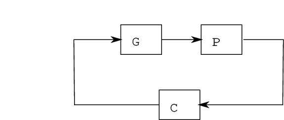
Figure 7: Feedback interconnection of a linear plant 𝐆\mathbf{G}, controller 𝐂\mathbf{C} and hysteresis operator 𝚽{\bf\Phi}. (a) An interconnection example where the plant 𝐆\mathbf{G} is driven by a hysteretic actuator 𝚽\mathbf{\Phi}; (b) An interconnection example where the dynamics of 𝐆\mathbf{G} is measured by a hysteretic sensor 𝚽\mathbf{\Phi}.

VI Controller design

The stability analysis given in the previous sections can be used to design a controller for a linear plant with hysteretic sensor/actuator. Consider the closed-loop system as shown in Figure 7, where 𝐆\mathbf{G} and 𝐂\mathbf{C} are the linear plant and controller, respectively, and they are given by

𝐆:{x˙G=AG​xG+BG​uG,yG=CG​xG+DG​uG,​𝐂:{x˙C=AC​xC+BC​uC,yC=CC​xC+DC​uC.\mathbf{G}:\left\{\begin{array}[]{rl}\dot{x}_{G}&=A_{G}x_{G}+B_{G}u_{G},\\ y_{G}&=C_{G}x_{G}+D_{G}u_{G},\end{array}\right.\ \mathbf{C}:\left\{\begin{array}[]{rl}\dot{x}_{C}&=A_{C}x_{C}+B_{C}u_{C},\\ y_{C}&=C_{C}x_{C}+D_{C}u_{C}.\end{array}\right. (58)

Thus depending on the location of the hysteretic element, the cascaded linear systems can be compactly written into

x˙=A​x+B​uy=C​x+D​u,\left.\begin{array}[]{rl}\dot{x}&=Ax+Bu\\ y&=Cx+Du,\end{array}\right. (59)

where x=[xGxC]x=\left[\begin{smallmatrix}x_{G}\\ x_{C}\end{smallmatrix}\right] and for the case of hysteretic actuator as shown in Figure 7(a), A=[AG0BC​CGAC]A=\left[\begin{smallmatrix}A_{G}&0\\ B_{C}C_{G}&A_{C}\end{smallmatrix}\right], B=[BGBC​DG]B=\left[\begin{smallmatrix}B_{G}\\ B_{C}D_{G}\end{smallmatrix}\right], C=[DC​CGCC]C=\left[\begin{smallmatrix}D_{C}C_{G}&C_{C}\end{smallmatrix}\right], D=DC​DGD=D_{C}D_{G}, or for the case of hysteretic sensor as shown in Figure 7(b), A=[AGBG​CC0AC]A=\left[\begin{smallmatrix}A_{G}&B_{G}C_{C}\\ 0&A_{C}\end{smallmatrix}\right], B=[BG​DCBC]B=\left[\begin{smallmatrix}B_{G}D_{C}\\ B_{C}\end{smallmatrix}\right], C=[CGDG​CC]C=\left[\begin{smallmatrix}C_{G}&D_{G}C_{C}\end{smallmatrix}\right], D=DG​DCD=D_{G}D_{C}. The controller design can then be carried out as follows.

  • •

    Control design algorithm for the case of CCW Φ\Phi:

    1. 1.

      Determine the anhysteresis function fa​nf_{an} of the Duhem operator Φ\Phi and possibly, the desired LL.

    2. 2.

      Find 𝐂\mathbf{C} such that either (36)-(38) or (41)-(42) holds.

    3. 3.

      If (36)-(38) is solvable, then 𝐂\mathbf{C} stabilizes the closed-loop system with a negative feedback interconnection; otherwise

    4. 4.

      If (41)-(42) is solvable, then 𝐂\mathbf{C} stabilizes the closed-loop system with a positive feedback interconnection.

  • •

    Control design algorithm for the case of CW Φ\Phi:

    1. 1.

      Determine the functions f1f_{1} and f2f_{2} of the Duhem operator Φ\Phi and possibly, the desired LL.

    2. 2.

      Find 𝐂\mathbf{C} such that either (50)-(51) or (53)-(54) holds.

    3. 3.

      If (50)-(51) is solvable, then 𝐂\mathbf{C} stabilizes the closed-loop system with a negative feedback interconnection; otherwise

    4. 4.

      If (53)-(54) is solvable, then 𝐂\mathbf{C} stabilizes the closed-loop system with a positive feedback interconnection.

Putting (59) into the setting of our main results in Theorem IV.3, IV.1, V.1 and V.3, the invariant set is contained in M:={(xG,xC,yΦ)|N⁡[xGxCyΦ]=0}M:=\{(x_{G},x_{C},y_{\Phi})|N\left[\begin{smallmatrix}x_{G}\\ x_{C}\\ y_{\Phi}\end{smallmatrix}\right]=0\} where the matrix NN can also become a design parameter for determining 𝐂\mathbf{C}.

VII Numerical examples

Refer to caption
Figure 8: Mass-damper-spring system connected with a hysteretic actuator

As an example, we consider a mass-damper-spring system with a hysteretic actuator denoted by Φ\Phi, as shown in Figure 8, where mm is the mass, bb is the damping constant, kk is the spring constant and xx denotes the displacement of the mass. Let m=1m=1, b=2b=2 and k=1k=1, then the mass-damper-spring system is given by

x˙\displaystyle\dot{x} =(01−1−2)​x+(01)​u,\displaystyle=\left(\begin{array}[]{cc}0&1\\ -1&-2\\ \end{array}\right)x+\left(\begin{array}[]{c}0\\ 1\\ \end{array}\right)u,
y\displaystyle y =(10)​x+u.\displaystyle=\left(\begin{array}[]{cc}1&0\\ \end{array}\right)x+u.

VII-A CCW hysteretic actuator

Let us first consider the case when the hysteretic actuator has CCW I/O dynamics, such as piezo-actuators [15]. Assume that the actuator is represented by the Duhem operator (14) where

f1​(γ,v)=−γ+0.475​v+0.3,f2​(γ,v)=γ−0.475​v+0.3,∀(γ,v)∈ℝ2.f_{1}(\gamma,v)=-\gamma+0.475v+0.3,\ f_{2}(\gamma,v)=\gamma-0.475v+0.3,\ \forall(\gamma,v)\in{\mathbb{R}}^{2}. (65)

It can be verified that fa​n​(v)=0.475​vf_{an}(v)=0.475v and the functions f1f_{1} and f2f_{2} satisfy the hypotheses given in Theorem III.1.

With Ac=[01−2−4]A_{c}=\left[\begin{smallmatrix}0&1\\ -2&-4\end{smallmatrix}\right], Bc=[01]B_{c}=\left[\begin{smallmatrix}0\\ 1\end{smallmatrix}\right], Cc=[−1.5−2]C_{c}=\left[\begin{smallmatrix}-1.5&-2\end{smallmatrix}\right] and Dc=1D_{c}=1, conditions (41)-(42) are solvable with P=[110−1.5−217.745.51−8.74−15.8605.517.4−5.51−14.36−1.5−8.74−5.5110.2417.86−2−15.86−14.3617.8638.36]P=\left[\begin{smallmatrix}1&1&0&-1.5&-2\\ 1&7.74&5.51&-8.74&-15.86\\ 0&5.51&7.4&-5.51&-14.36\\ -1.5&-8.74&-5.51&10.24&17.86\\ -2&-15.86&-14.36&17.86&38.36\end{smallmatrix}\right] and L=[0 0 1/4 0 0]L=[0\ 0\ 1/4\ 0\ 0]. Hence the controller 𝐂\mathbf{C} can stabilize the closed-loop system with negative feedback interconnection. In this case, N=[0 1/4 0 0 0]N=[0\ 1/4\ 0\ 0\ 0]. According to Theorem IV.3, the velocity of the mass-damper-spring system converges to zero and the position of the mass-damper-spring system converges to a constant. The closed-loop system is simulated in Matlab/Simulink with the initial condition x⁡(0)=[−10 5]Tx(0)=[-10\ 5]^{T} and the results are shown in Figure 9(a).

On the other hand, since we have fa​n​(v)=0.475​vf_{an}(v)=0.475v, then by taking Ac=[01−2−4]A_{c}=\left[\begin{smallmatrix}0&1\\ -2&-4\end{smallmatrix}\right], Bc=[01]B_{c}=\left[\begin{smallmatrix}0\\ 1\end{smallmatrix}\right], Cc=[11]C_{c}=\left[\begin{smallmatrix}1&1\end{smallmatrix}\right] and Dc=0D_{c}=0, it can be checked that (36)-(37) holds with ξ=0.5\xi=0.5 and Q=[61−6−214−1−4−6−173−2−437]Q=\left[\begin{smallmatrix}6&1&-6&-2\\ 1&4&-1&-4\\ -6&-1&7&3\\ -2&-4&3&7\end{smallmatrix}\right]. In this case N=[10−2−31]N=\left[\begin{smallmatrix}1&0&-2&-3&1\end{smallmatrix}\right]. Moreover, fa​nf_{an} belongs to the sector [0,0.5][0,0.5]. Similar to the previous case, it follows from Theorem IV.1 that the velocity of the mass-damper-spring system converges to zero and the position of the mass-damper-spring system converges to a constant. The simulation results is shown in Figure 9(b).

Refer to caption
Refer to caption
Figure 9: Simulation results of the numerical example with CCW hysteretic actuator. (a) The negative feedback interconnection case with the initial condition x⁡(0)=[−10 5]Tx(0)=[-10\ 5]^{T}; (b) The positive feedback interconnection case with the initial condition x⁡(0)=[−10 10]Tx(0)=[-10\ 10]^{T}.

VII-B CW hysteretic actuator

For the case of a CW hysteretic actuator, see for example the magnetorheological (MR) damper used in the structure control [25], the mass-damper-spring system is given by (VII). Assume that the actuator is represented by the Duhem operator (14) where

f1​(γ,v)=0.25​(1−γ),f2​(γ,v)=0.25​(1+γ),∀(γ,v)∈ℝ2.f_{1}(\gamma,v)=0.25(1-\gamma),\ f_{2}(\gamma,v)=0.25(1+\gamma),\ \forall(\gamma,v)\in{\mathbb{R}}^{2}. (66)

The anhysteresis function for this Duhem operator is fa​n=0f_{an}=0. It can be shown that f1≤0.25f_{1}\leq 0.25 and f2≤0.25f_{2}\leq 0.25 for all v∈ℝv\in{\mathbb{R}}. In addition f1f_{1} and f2f_{2} satisfy the hypotheses in Theorem III.3, hence the Duhem operator with (66) is CW.

With Ac=[01−2−4]A_{c}=\left[\begin{smallmatrix}0&1\\ -2&-4\end{smallmatrix}\right], Bc=[01]B_{c}=\left[\begin{smallmatrix}0\\ 1\end{smallmatrix}\right], Cc=[11]C_{c}=\left[\begin{smallmatrix}1&1\end{smallmatrix}\right] and Dc=0D_{c}=0, the conditions (50)-(51) are solvable with P=[51−5−213−1−3−5−163−2−336]P=\left[\begin{smallmatrix}5&1&-5&-2\\ 1&3&-1&-3\\ -5&-1&6&3\\ -2&-3&3&6\end{smallmatrix}\right]. Hence the controller 𝐂\mathbf{C} can stabilize the closed-loop system with negative feedback interconnection. In this case, N=[1 0−2−3 1]N=[1\ 0\ -2\ -3\ 1]. According to Theorem V.1, the velocity of the mass-damper-spring system converges to zero and the position of the mass-damper-spring system converges to a constant. The simulation results are shown in Figure 10(a) with the initial condition x⁡(0)=[10 5]Tx(0)=[10\ 5]^{T}.

Since we have f1≤0.25f_{1}\leq 0.25 and f2≤0.25f_{2}\leq 0.25 for all v∈ℝv\in{\mathbb{R}}, by taking Ac=[01−2−3]A_{c}=\left[\begin{smallmatrix}0&1\\ -2&-3\end{smallmatrix}\right], Bc=[01]B_{c}=\left[\begin{smallmatrix}0\\ 1\end{smallmatrix}\right], Cc=[−3−1]C_{c}=\left[\begin{smallmatrix}-3&-1\end{smallmatrix}\right] and Dc=2D_{c}=2, it can be checked that (53)-(54) holds with δ=1\delta=1, η=0.5\eta=0.5, L=[01/4000]L=\left[\begin{smallmatrix}0&1/4&0&0&0\end{smallmatrix}\right] and P=[220−3−1230.8615.83−32.86−26.9015.8338.26−15.83−51.4−3−32.86−15.8335.8627.9−1−26.9−51.427.974.54]P=\left[\begin{smallmatrix}2&2&0&-3&-1\\ 2&30.86&15.83&-32.86&-26.9\\ 0&15.83&38.26&-15.83&-51.4\\ -3&-32.86&-15.83&35.86&27.9\\ -1&-26.9&-51.4&27.9&74.54\end{smallmatrix}\right]. It follows from Theorem V.3 that the velocity of the mass-damper-spring system converges to zero and the position of the mass-damper-spring system converges to a constant. The simulation results is shown in Figure 10(b).

Refer to caption
Refer to caption
Figure 10: Simulation results of the numerical example with CW hysteretic actuator. (a) The negative feedback interconnection case with the initial condition x⁡(0)=[10 5]Tx(0)=[10\ 5]^{T}; (b) The positive feedback interconnection case with the initial condition x⁡(0)=[10−5]Tx(0)=[10\ -5]^{T}.

VIII Conclusions

It has been shown in this paper that the stability analysis of a linear system with hysteresis nonlinearity is accommodated by exploiting the I/O property of the corresponding hysteresis operator. Furthermore, the stability analysis enables a straightforward control design methodology for a plant with hysteresis nonlinearity without having to know precisely the parameters of the hysteresis operator. It offers a different paradigm in the design of controller for such systems where we do not need to define an inverse hysteresis operator which is commonly used in practice. The dissipativity approach which is used in this paper can be extended directly to nonlinear plants with hysteresis nonlinearity. One possible class of nonlinear plants which can be treated with our approach is the CCW systems as studied by Angeli [1] and by van der Schaft [26].

References

  • [1] D. Angeli, “Systems with Counterclockwise Input-Output Dynamics”, IEEE Transactions on Automatic Control, vol. 51, no. 7, pp. 1130-1143, 2006.
  • [2] D. Angeli, “Multistability in Systems with Counter-clockwise Input-Ouput Dynamics”, IEEE Transactions on Automatic Control, vol. 52, no. 4, pp. 596-609, 2007.
  • [3] G. Bertotti & I. D. Mayergoyz, The Science of Hysteresis: Mathematical Modeling and Applications, Academic Press, San Diego, 2006.
  • [4] M. Brokate & J. Sprekels, Hysteresis and Phase Transitions, Springer Verlag, New York, 1996.
  • [5] Bernard. D. Coleman, Marion. L. Hodgdon, “A Constitutive Relation for Rate-independent Hysteresis in Ferromagnetically Soft Materials”, International Journal of Engineering Science, vol. 24, no. 6, pp. 897-919, 1986.
  • [6] P. Dahl, “Solid Friction Damping of Mechanical Vibrations”, AIAA J., vol. 14, no. 2, pp. 1675-1682, 1976.
  • [7] D. Damjanovic, Hysteresis in Piezoelectric and Ferroelectric Materials, The Science of Hysteresis, I. Mayergoyz and G. Bertotti (editors), vol. 3, 2005.
  • [8] R.B. Gorbet, K.A. Morris, “Generalized Dissipation in Hysteretic Systems”, Proc. IEEE Conf. Dec. Contr., Tampa, 1998.
  • [9] B. Jayawardhana, V. Andrieu, “Sufficient Conditions for Dissipativity on Duhem Hysteresis Model”, Proc. IEEE Conf. Dec. Contr., Shanghai, 2009.
  • [10] B. Jayawardhana, Ruiyue Ouyang, V. Andrieu, “Dissipativity of General Duhem Hysteresis Models”, Proc. IEEE Conf. Dec. Contr., Orlando, 2011.
  • [11] B. Jayawardhana, Ruiyue Ouyang, V. Andrieu, “Stability of Systems with Duhem Hysteresis Operator: Dissipativity Approach”, Automatica, To appear.
  • [12] D. C. Jiles, D. L. Atherton, “Theory of Ferromagnetic Hysteresis”, Journal of Magnetism and Magnetic Material, vol. 61, no. 1-2, pp. 48-6, 1986.
  • [13] T. Kamada, T. Fujita, T. Hatayama, T. Arikabe, N. Murai, S. Aizawa and K. Tohyama, “Active Vibration Control of Frame Structures with Smart Structures using Piezoelectric Actuators”, Journal of Smart Material and Structures, vol. 6, no. 4, pp. 448-456, 1997.
  • [14] H.K. Khalil. Nonlinear Systems, 3rd edition, Prentice-Hall, Upper Saddle River, NJ, 2002.
  • [15] C. J. Lin, S. R. Yang, “Precise Positioning of Piezo-actuated Stages using Hysteresis-observer based Control”, Mechatronics, vol. 16, no. 7, pp. 417-426, 2006.
  • [16] H. Logemann & E.P. Ryan, “Systems with Hysteresis in the Feedback Loop: Existence, Regularity and Asymptotic Behaviour of Solutions”, ESAIM Control, Optimiz. & Calculus of Variations, vol. 9, pp. 169-196, 2003.
  • [17] H. Logemann, E. P. Ryan, “Asymptotic Behaviour of Nonlinear Systems”, American Mathematical Monthly, vol. 111, no. 10, pp. 864-889, 2004.
  • [18] J. W. Macki, P. Nistri, P. Zecca, “Mathematical Models for Hysteresis”, SIAM Review, vol. 35, no. 1, pp. 94–123, 1993.
  • [19] J. Oh, D. S. Bernstein, “Semilinear Duhem Model for Rate-independent and Rate-dependent Hysteresis”, IEEE Trans. Automat. Contr., vol. 50, no. 5, pp. 631–645, 2005.
  • [20] A. K. Padthe, J. Oh and D. S. Bernstein, “Counterclockwise Dynamics of a Rate-independent Semilinear Duhem Model”, Proc. IEEE Conf. Dec. Contr., Seville, 2005.
  • [21] A. K. Padthe, B. Drincic, J. Oh, D. D. Rizos, S. D. Fassois and D. S. Bernstein, “Duhem modeling of Friction-Induced Hysteresis”, IEEE Control System Magazine, vol. 28, no. 5, pp. 90-107, 2008.
  • [22] T. Pare, A. Hassabi and J. J. How, “A KYP Lemma and Invariance Principle for Systems with Multiple Hysteresis Non-linearities”, Int. J. Contr.,vol. 74, no. 11, pp. 1140-1157, 2001.
  • [23] I. R. Petersen and A. Lanzon, “Feedback Control of Negative-imaginary System”, IEEE Control System Magazine, vol. 30, no. 5, pp. 54-72, 2010.
  • [24] R. Ouyang, V. Andrieu, Bayu Jayawardhana, “On the Characterization of the Duhem Hysteresis Operator with Clockwise Input-Output Dynamics”, submitted, http://arxiv.org/abs/1201.2035.
  • [25] C. Sakai, H. Ohmori, A. Sano “Modeling of MR Damper with Hysteresis for Adaptive Vibration Control”, Proc. IEEE Conf. Dec. Contr., Maui, 2003.
  • [26] A.J. van der Schaft, “Positive Feedback Interconnection of Hamiltonian Systems”, Proc. IEEE Conf. Dec. Contr., Orlando, 2011.
  • [27] S. Tarbouriech, I. Queinnec, C. Prieur, “Stability Analysis and Stabilization of Systems with Backlash in the Feedback Loop”, IEEE Transactions on Automatic Control, submitted.
  • [28] A. Visintin, Differential Models of Hysteresis, Springer-Verlag, New York, 1994.
  • [29] J. C. Willems, “Dissipative Dynamical Systems. Part I: General Theory. Part II: Linear Systems with Quadratic Supply Rates”, Arch. Rat. Mech. Anal., vol. 45, no. 5, pp. 321-393, 1972.