CERN-OPEN-2012-015
LHeC-Note-2012-002 GEN
Geneva, June 13, 2012
![[Uncaptioned image]](1206.2913v2/AN_cernlogo.png)
A Large Hadron Electron Collider
at CERN
Report on the Physics and Design
Concepts for Machine and Detector
LHeC Study Group
![[Uncaptioned image]](1206.2913v2/satkand.png)
The Kandinsky painting, “Circles in a circle” (1923), is taken from a talk on gluon saturation and black hole duality as presented at the first CERN-ECFA-NuPECC Workshop on the LHeC held at Divonne near to CERN in September 2008 [1]. We thank the Philadelphia Museum of Art, USA, for the permission to reproduce it here.
Kreise im Kreis, 923 (R.702), Vassily Kandinsky
Oil on canvas, 38 7/8 x 37 5/8 inches (98.7 x 95.6 cm)
Philadelphia Museum of Art: The Louise and Walter Arensberg Collection, 1950
©ADAGP, Paris and DACS, London 2012.
Abstract
The physics programme and the design are described of a new collider for particle and nuclear physics, the Large Hadron Electron Collider (LHeC), in which a newly built electron beam of GeV, to possibly GeV, energy collides with the intense hadron beams of the LHC. Compared to the first collider, HERA, the kinematic range covered is extended by a factor of twenty in the negative four-momentum squared, , and in the inverse Bjorken , while with the design luminosity of cm-2s-1 the LHeC is projected to exceed the integrated HERA luminosity by two orders of magnitude. The physics programme is devoted to an exploration of the energy frontier, complementing the LHC and its discovery potential for physics beyond the Standard Model with high precision deep inelastic scattering measurements. These are designed to investigate a variety of fundamental questions in strong and electroweak interactions. The LHeC thus continues the path of deep inelastic scattering (DIS) into unknown areas of physics and kinematics. The physics programme also includes electron-deuteron and electron-ion scattering in a range extended by four orders of magnitude as compared to previous lepton-nucleus DIS experiments for novel investigations of neutron’s and nuclear structure, the initial conditions of Quark-Gluon Plasma formation and further quantum chromodynamic phenomena. The LHeC may be realised either as a ring-ring or as a linac-ring collider. Optics and beam dynamics studies are presented for both versions, along with technical design considerations on the interaction region, magnets including new dipole prototypes, cryogenics, RF, and further components. A design study is also presented of a detector suitable to perform high precision DIS measurements in a wide range of acceptance using state-of-the art detector technology, which is modular and of limited size enabling its fast installation. The detector includes tagging devices for electron, photon, proton and neutron detection near to the beam pipe. Civil engineering and installation studies are presented for the accelerator and the detector. The LHeC can be built within a decade and thus be operated while the LHC runs in its high-luminosity phase. It so represents a major opportunity for progress in particle physics exploiting the investment made in the LHC.
LHeC Study Group
J.L.Abelleira Fernandez16,23, C.Adolphsen57, A.N.Akay03, H.Aksakal39, J.L.Albacete52, S.Alekhin17,54, P.Allport24, V.Andreev34, R.B.Appleby14,30, E.Arikan39, N.Armesto53,a, G.Azuelos33,64, M.Bai37, D.Barber14,17,24, J.Bartels18, O.Behnke17, J.Behr17, A.S.Belyaev15,56, I.Ben-Zvi37, N.Bernard25, S.Bertolucci16, S.Bettoni16, S.Biswal41, J.Blümlein17, H.Böttcher17, A.Bogacz36, C.Bracco16, G.Brandt44, H.Braun65, S.Brodsky57,b, O.Brüning16, E.Bulyak12, A.Buniatyan17, H.Burkhardt16, I.T.Cakir02, O.Cakir01, R.Calaga16, V.Cetinkaya01, E.Ciapala16, R.Ciftci01, A.K.Ciftci01, B.A.Cole38, J.C.Collins48, O.Dadoun42, J.Dainton24, A.De.Roeck16, D.d’Enterria16, A.Dudarev16, A.Eide60, R.Enberg63, E.Eroglu62, K.J.Eskola21, L.Favart08, M.Fitterer16, S.Forte32, A.Gaddi16, P.Gambino59, H.García Morales16, T.Gehrmann69, P.Gladkikh12, C.Glasman28, R.Godbole35, B.Goddard16, T.Greenshaw24, A.Guffanti13, V.Guzey19,36, C.Gwenlan44, T.Han50, Y.Hao37, F.Haug16, W.Herr16, A.Hervé27, B.J.Holzer16, M.Ishitsuka58, M.Jacquet42, B.Jeanneret16, J.M.Jimenez16, J.M.Jowett16, H.Jung17, H.Karadeniz02, D.Kayran37, A.Kilic62, K.Kimura58, M.Klein24, U.Klein24, T.Kluge24, F.Kocak62, M.Korostelev24, A.Kosmicki16, P.Kostka17, H.Kowalski17, G.Kramer18, D.Kuchler16, M.Kuze58, T.Lappi21,c, P.Laycock24, E.Levichev40, S.Levonian17, V.N.Litvinenko37, A.Lombardi16, J.Maeda58, C.Marquet16, S.J.Maxfield24, B.Mellado27, K.H.Mess16, A.Milanese16, S.Moch17, I.I.Morozov40, Y.Muttoni16, S.Myers16, S.Nandi55, Z.Nergiz39, P.R.Newman06, T.Omori61, J.Osborne16, E.Paoloni49, Y.Papaphilippou16, C.Pascaud42, H.Paukkunen53, E.Perez16, T.Pieloni23, E.Pilicer62, B.Pire45, R.Placakyte17, A.Polini07, V.Ptitsyn37, Y.Pupkov40, V.Radescu17, S.Raychaudhuri35, L.Rinolfi16, R.Rohini35, J.Rojo16,31, S.Russenschuck16, M.Sahin03, C.A.Salgado53,a, K.Sampei58, R.Sassot09, E.Sauvan04, U.Schneekloth17, T.Schörner-Sadenius17, D.Schulte16, A.Senol22, A.Seryi44, P.Sievers16, A.N.Skrinsky40, W.Smith27, H.Spiesberger29, A.M.Stasto48,d, M.Strikman48, M.Sullivan57, S.Sultansoy03,e, Y.P.Sun57, B.Surrow11, L.Szymanowski66,f, P.Taels05, I.Tapan62, A.T.Tasci22, E.Tassi10, H.Ten.Kate16, J.Terron28, H.Thiesen16, L.Thompson14,30, K.Tokushuku61, R.Tomás García16, D.Tommasini16, D.Trbojevic37, N.Tsoupas37, J.Tuckmantel16, S.Turkoz01, T.N.Trinh47, K.Tywoniuk26, G.Unel20, J.Urakawa61, P.VanMechelen05, A.Variola52, R.Veness16, A.Vivoli16, P.Vobly40, J.Wagner66, R.Wallny68, S.Wallon43,46,f, G.Watt16, C.Weiss36, U.A.Wiedemann16, U.Wienands57, F.Willeke37, B.-W.Xiao48, V.Yakimenko37, A.F.Zarnecki67, Z.Zhang42, F.Zimmermann16, R.Zlebcik51, F.Zomer42
01 Ankara University, Turkey
02 SANAEM Ankara, Turkey
03 TOBB University of Economics and Technology, Ankara, Turkey
04 LAPP, Annecy, France
05 University of Antwerp, Belgium
06 University of Birmingham, UK
07 INFN Bologna, Italy
08 IIHE, Université Libre de Bruxelles, Belgium, supported by the FNRS
09 University of Buenos Aires, Argentina
10 INFN Gruppo Collegato di Cosenza and Universita della Calabria, Italy
11 Massachusetts Institute of Technology, Cambridge, USA
12 Charkow National University, Ukraine
13 University of Copenhagen, Denmark
14 Cockcroft Institute, Daresbury, UK
15 Rutherford Appleton Laboratory, Didcot, UK
16 CERN, Geneva, Switzerland
17 DESY, Hamburg and Zeuthen, Germany
18 University of Hamburg, Germany
19 Hampton University, USA
20 University of California, Irvine, USA
21 University of Jyväskylä, Finland
22 Kastamonu University, Turkey
23 EPFL, Lausanne, Switzerland
24 University of Liverpool, UK
25 University of California, Los Angeles, USA
26 Lund University, Sweden
27 University of Wisconsin-Madison, USA
28 Universidad Autónoma de Madrid, Spain
29 University of Mainz, Germany
30 The University of Manchester, UK
31 INFN Milano, Italy
32 University of Milano, Italy
33 University of Montréal, Canada
34 LPI Moscow, Russia
35 Tata Institute, Mumbai, India
36 Jefferson Lab, Newport News, VA 23606, USA
37 Brookhaven National Laboratory, New York, USA
38 Columbia University, New York, USA
39 Nigde University, Turkey
40 Budker Institute of Nuclear Physics SB RAS, Novosibirsk, 630090 Russia
41 Orissa University, India
42 LAL, Orsay, France
43 Laboratoire de Physique Théorique, Université Paris XI, Orsay, France
44 University of Oxford, UK
45 CPHT, École Polytechnique, CNRS, 91128 Palaiseau, France
46 UPMC University of Paris 06, Faculté de Physique, Paris, France
47 LPNHE University of Paris 06 and 07, CNRS/IN2P3, 75252 Paris, France
48 Pennsylvania State University, USA
49 University of Pisa, Italy
50 University of Pittsburgh, USA
51 Charles University, Praha, Czech Republic
52 IPhT Saclay, France
53 University of Santiago de Compostela, Spain
54 Serpukhov Institute, Russia
55 University of Siegen, Germany
56 University of Southampton, UK
57 SLAC National Accelerator Laboratory, Stanford, USA
58 Tokyo Institute of Technology, Japan
59 University of Torino and INFN Torino, Italy
60 NTNU, Trondheim, Norway
61 KEK, Tsukuba, Japan
62 Uludag University, Turkey
63 Uppsala University, Sweden
64 TRIUMF, Vancouver, Canada
65 Paul Scherrer Institute, Villigen, Switzerland
66 National Center for Nuclear Research (NCBJ), Warsaw, Poland
67 University of Warsaw, Poland
68 ETH Zurich, Switzerland
69 University of Zurich, Switzerland
a supported by European Research Council grant HotLHC ERC-2011-StG-279579 and
MiCinn of Spain grants FPA2008-01177, FPA2009-06867-E and Consolider-Ingenio 2010 CPAN CSD2007-00042,
Xunta de Galicia grant PGIDIT10PXIB206017PR, and FEDER.
b supported by the U.S. Department of Energy,contract DE–AC02–76SF00515.
c supported by the Academy of Finland, project no. 141555.
d supported by the Sloan Foundation,
DOE OJI grant No. DE - SC0002145 and
Polish NCN grant DEC-2011/01/B/ST2/03915.
e supported by the Turkish Atomic Energy Authority (TAEK).
f supported by the P2IO consortium.
Foreword
The traditions of CERN on deep inelastic lepton-hadron scattering date back to the discovery of weak neutral currents by the Gargamelle collaboration and, subsequently, the exploration of the valence and sea-quark contents of the nucleon, tests of Quantum Chromodynamics and electroweak phenomena and the observation of unexpected effects in the behaviour of quarks in protons and nuclei, made in a series of neutrino and muon scattering experiments. Following HERA, the first electron-proton collider built at DESY, with the LHeC there is an opportunity for energy frontier deep inelastic scattering to return to CERN in order to enrich the physics which has been made accessible by the Large Hadron Collider. Using a novel high energy electron beam scattered off LHC protons and also ions, the LHeC would represent the cleanest high resolution microscope in the world, based on new principles which deserve to be developed. The design report, available herewith, covering concepts of the accelerator and detector, together with an evaluation of the physics potential, had been initiated by the CERN Science Policy Committee and been worked out by an international study group, supported by CERN, the European Committee for Future Accelerators, ECFA, and the Nuclear Physics European Collaboration Committee, NuPECC.
The report describes a challenging new opportunity for European and
global particle physics. Looking forward to the further development of
the LHeC project, CERN with international partners is now evaluating
ways of cooperation towards technical designs of the highest energy
electron linac, with power recovery, and of a new detector which
would enable ultra-precise, large acceptance deep inelastic scattering
measurements. By the time the LHC will provide its first luminous
results at the design beam energy, in around 2015, a possible upgrade
of the LHC as is proposed here may advance. For now, CERN has to thank
the scientists and engineers involved, the members of the Scientific
Advisory Committee, of ECFA and NuPECC and especially the many expert
referees which in the final phase of this study helped in scrutinising
the LHeC design.
Sergio Bertolucci (Director of Research and Computing of CERN)
Preface
Preparations for new, big machines take time. The idea of an electron-proton () collider in the LEP-LHC tunnel was discussed as early as 1984 [2], at the first LHC workshop at Lausanne. This was the time when the first ever built collider, HERA, was approved by the German government. HERA was a machine of about GeV electron beam energy and nearly TeV proton beam energy, a combination of a warm dipole electron ring with a superconducting dipole proton ring, in a km circumference tunnel. The machine started operation years after its approval. It reached luminosities of cm-2s-1 in its first phase of operation which were increased by about a factor of in the subsequent, upgraded configuration. HERA never attempted to collide electrons with deuterons nor with ions.
The realisation of HERA at DESY had followed a number of attempts to realise interactions in collider mode, mainly driven by the unforgettable Bjoern Wiik: since the late 1960s, he and his colleagues had considered such machines and proposed to probe the proton’s structure more deeply with an collider at DORIS [3], later at PETRA (PROPER) [4] and subsequently at the SPS at CERN (CHEEP) [5]. Further collider studies were made for PEP [6], TRISTAN [7] and also the Tevatron (CHEER) [8].
In 1990, at a workshop at Aachen, the combination of LEP with the LHC was discussed, with studies [9, 10, 11] on the luminosity, interaction region, a detector and the physics as seen with the knowledge of that time, before HERA. Following a request of the CERN Science Policy Committee (SPC), a brief study of the ring-ring collider in the LEP tunnel was performed [12] leading to an estimated luminosity of about cm-2s-1.
At the end of the eighties it had been anticipated that there was a possible end to the increase of the energy of colliders in the ring-ring configuration, because of the synchrotron radiation losses of an electron ring accelerator. The classic SLAC fixed target experiment had already used a mile linac. For linac-ring collider configurations, two design sketches considering electron beam energies up to a few hundred GeV were published, in 1988 [13] and in 1990 [14]. As part of the TESLA linear collider proposal, an option (THERA) was studied [15] to collide electrons of a few hundred GeV energy with protons and ions from HERA. Later, in 2003, the possibility was evaluated to combine LHC protons with CLIC electrons [16]. It was yet realised, that the bunch structures of the LHC and CLIC were not compliant with the need for high luminosities.
In September 2007, the SPC again asked whether one could realise an collider at CERN. Some of us had written a paper [17] in the year before, that had shown in detail, for the first time, that a luminosity of cm-2s-1 was achievable. This appeared possible in a ring-ring configuration based on the “ultimate” LHC beam, with protons in bunches ns apart. Thanks to the small beam-beam tune-shift, it was found to be feasible to simultaneously operate in the LHC and in the new machine, which in 2005 was termed the Large Hadron Electron Collider (LHeC) [18]. Thus it appeared possible to realise an collider that was complementary to the LHC, just as HERA was to the Tevatron. The integrated luminosity was projected to be O(100) fb-1, a factor of a hundred more than HERA had collected over its lifetime of 15 years.
It was clear that with a centre-of-mass energy of about TeV an exciting programme of deep inelastic scattering (DIS) measurements at the energy-frontier was in reach. This would comprise searches and analyses for physics beyond the Standard Model, novel measurements in QCD and electroweak physics to unprecedented precision, as well as DIS physics at such low Bjorken , that all the known laws of parton and gluon interactions would have to be modified to account for non-linear parton interaction effects. It had also been realised that the kinematic region, in terms of negative four-momentum-transfer squared, , and , accessed in lepton-nucleus interactions could be extended by orders of magnitude using the ion beams of the LHC. A salient theme of the LHeC therefore is the precise mapping of the gluon field, over six orders of magnitude in Bjorken , in protons, neutrons and nuclei, with unprecedented sensitivity.
In the autumn of 2007, (r)ECFA and CERN invited us to work out the LHeC concept to a degree, which would allow one to understand its physics programme, evaluate the accelerator options and their technical realisation. The detector design should be affordable and capable of realising a high precision, large acceptance experimental programme of deep inelastic scattering at the energy frontier. The electron beam energy range was set to be between about GeV. The wall plug power consumed for the electron beam was limited to MW.
For the installation of the LHC it had been decided to remove LEP from the tunnel and to re-use the injector chain. To realise an collider based on the LHC, a new electron accelerator has to be built. The following report details two solutions for the chosen default electron beam energy of GeV. One option is to build and install a new ring, with modern magnet technology, on top of the LHC, using a new GeV injector. Alternatively, one can build a “linac”, actually two GeV superconducting linacs in a racetrack configuration. By employing energy recovery techniques, this configuration could provide the equivalent of about GW available power and reach cm-2s-1 luminosity. The LHeC linac would be of about the same length as the one used for the discovery of quarks at SLAC [19, 20], but capable of probing parton interactions with a exceeding that of the 1969 machine by a factor of nearly .
It was agreed early on to devote a few years to the report, also because none of the people involved could work anything near to full time for this endeavour. Three workshops were held in 2008-2010, that annually assembled about a hundred experts on theory, experiment and accelerator to develop the LHeC design concepts. The project was presented annually to ECFA and in 2008 to ICFA, see [21]. In view of the unique electron-ion scattering programme of the LHeC, the design effort became also supported by NuPECC, and the LHeC is now part of the NuPECC roadmap for European nuclear physics as released in 2010 [22]. Following an intermediate report to the Science Policy Committee of CERN, in July 2010, the SPC considered the LHeC “an option for a future project at CERN”.
In August 2011, a first complete draft of this conceptual design report was handed to more than twenty experts on various aspects of the physics and technology of the LHeC, which CERN had invited to referee the project and scrutinise its motivation and its design. The report has been completed following often close interactions with the referees and due consideration of their observations.
The LHeC by its nature is an upgrade of the LHC. It substantially enriches the physics harvest related to the gigantic investment in the LHC. Whatever the outcome of the searches at the LHC for physics beyond the Standard Model turns out to be, an collider operating at the energy frontier is guaranteed to deepen the understanding of TeV scale physics and thus will support the development of the theory of elementary particles and their interactions.
The LHeC needs the LHC proton and ion beams to be operational and so the design is made for synchronous and operation, as well as and , including deuterons. Should the LHC eventually be upgraded to even higher beam energy, beyond TeV per beam [23], or a new proton collider be built, it would open an even higher energy reach for also. There certainly is a future for deep inelastic scattering at the energy frontier. It is herewith envisaged to begin with the LS3 shutdown of the LHC, in the early twenties, likely leading into further decades. As Frank Wilczek put it, “one of the joys of our subject is the continuing of our culture that bridges continents and generations” [24].
Our science is driven by curiosity, by theoretical
expectations, sometimes too great, but also by experiment
and technology, and the authors of this study therefore hope that the LHeC
may be given the chance to contribute to the common
efforts of our community for a deeper understanding of nature.
Max Klein (Chair of the LHeC Steering Committee)
The present document is a detailed presentation of the physics, the accelerator options and a detector design comprising the LHeC project. It has been developed under the auspices and with support of CERN, ECFA and NuPECC, between 2008 and now. The paper is organised as follows:
, the introduction, summarises cornerstones of deep inelastic scattering and the main considerations for the design of the LHeC are summarised. The emphasis is on adding a GeV energy electron beam to the existing proton and ion beams of the LHC, in a manner which foresees the simultaneous and operation for the realisation of a luminous DIS programme while minimising the interference with the LHC.
presents selected subjects, with related simulation studies and theoretical considerations, in order to sketch the physics programme of the LHeC. These subjects are grouped into three main, though related areas: high precision QCD and electroweak physics, the physics of high parton densities at low Bjorken x, in protons and in nuclei, and finally the potential for searches for phenomena beyond the standard model and its relation to the LHC. It has rarely been possible, fortunately, to accurately predict nor to fully simulate the physics of a new machine at much enlarged energies. Equally, the subjects here presented are not supposed to cover the complete field as it is known today. However, for a new laboratory of particle physics as the LHeC represents, a broad view must be taken to what it most likely comprises.
is devoted to the accelerator design, with studies presenting the ring-ring and linac-ring concepts, optics etc. and in a third section the various technical systems which often are common to both accelerator options. The emphasis here is on an understanding of the main challenges and characteristics of both options and not on discussing their relative merits. The accelerator part is concluded with separate sections on the civil engineering and a tentative time schedule for the realisation of the LHeC within about the next ten years.
presents the design considerations for a detector with its challenging central part and further systems to tag forward nucleons and backward scattered electrons and photons, including a study for a high precision measurement of the lepton beam polarisation. The salient feature of the detector baseline design is its silicon tracker surrounded by an electromagnetic liquid argon calorimeter inside a superconducting coil which uses a tile hadron calorimeter for the flux return. The detector part concludes with a first study of the installation of the apparatus, with premounting on the surface, lowering and integration underground.
contains a summary of the main results and considerations of this report with the intention of providing a brief overview on the LHeC design and possible prospect. This design study has been organised jointly by a steering group and convenors for the various physics, accelerator and detector parts. It was accompanied by a scientific advisory committee. A first draft was handed to more than 20 referees, which were nominated by the CERN directorate for a detailed evaluation of the design and a corresponding update. The composition of these groups is listed below the summary of the paper. Various members of the advisory committee have made direct scientific contributions to the LHeC design as presented here. They therefore also appear among the authors of this study which are representing a group of nearly physicists and engineers from institutes.
While this report is being published, the first luminous results from the LHC have become available, and HERA publishes its final papers. The interest in a TeV energy scale DIS collider of high luminosity has grown. The LHeC development will continue with a view to come to a technical design within a few years.
Part I Introduction
Chapter 1 Lepton-Hadron Scattering
1.1 Development and contributions
It is almost exactly 100 years since the birth of the scattering experiment as a means of revealing the structure of matter. Geiger and Marsden’s experiment [25] and its interpretation by Rutherford [26] set the scene for a century of ever-deeper and more precise resolution of the constituents of the atom, the nucleus and the nucleon. Lepton-hadron scattering has played a crucial role in this exploration over the past 55 years. The finite radius of the proton of about fm was first established through elastic electron-proton scattering experiments [27]. Later, through deep inelastic electron proton scattering at Stanford [20, 19], proton structure was understood in terms of quarks, still the smallest known constituents of matter. With the discovery of Bjorken scaling of the proton structure function , its quark model interpretation, and the subsequent discovery of scaling violation in support of asymptotic freedom [28, 29], deep inelastic scattering (DIS) became a field of fundamental theoretical importance [30] to the understanding of the strong interaction. Precise measurements of the parton momentum distributions of the nucleon became a major testing ground for the selection and development of Quantum Chromodynamics (QCD) [31] as the appropriate theory of the strong interaction. Prior to these developments, the theory of strong interactions was of merely phenomenological nature, built around S matrix theory and general amplitude features and various concepts such as Regge, bootstrap or further models [32].
Quantum Chromodynamics is a Yang-Mills gauge theory, in which the interaction between confined quarks proceeds via coloured gluon exchange. With improved resolution, as provided by increased , quarks can be resolved as quarks radiating gluons, whilst gluons may split into quark-antiquark pairs or, due to the non-abelian nature of the underlying gauge field theory, into pairs of gluons [33, 34, 35]. The development of QCD calculations beyond leading order [36, 37] is one of the most remarkable recent achievements of particle physics theory supported by experiment. It leads to a consistent description of all perturbatively accessible hadron observables in DIS (and beyond), as has recently been established over the kinematic range accessible to HERA [38]. This includes the unexpected observation of deep inelastic diffractive scattering at HERA, where in a significant fraction of violent DIS interactions the proton remains intact, mediated by an exchange of vacuum quantum numbers which often is termed “Pomeron exchange”.
Despite previous successes, many fundamental areas of QCD have not been verified experimentally, with instantons [39] as only one example. Even the classic areas related to quarks and gluons have not been exploited as required due to limited precision, range and variation of initial conditions. Meanwhile the theory underlying DIS experiences further fundamental developments. Four-dimensional conformal field theory is seen to be related to superstring theory in the anti-de Sitter space in ten dimensions, which relates the supersymmetric pomeron to the graviton in this space [40]. The evolution of partons is expected to obey different laws than explored hitherto at HERA, as at small their interactions have to be damped for the occurrence of non-linear interactions and possibly the restoration of unitarity, see [41] for a review.
Particle physics in the past could profit very much from the complementarity of hadron-hadron, DIS and experiments. Key observations were made in all three areas, and the overlap in physics coverage was used to achieve confidence in new and precision results. This is sketched in Figure 1.1 for the experiments of the seventies and eighties, which resulted in the birth of the Standard Model. Fig. 1.2 illustrates this for the experiments of the nineties until now, when the Tevatron, HERA and the SLC/LEP machines determined the progress in the exploration of particle physics at the energy frontier accessed with colliders. The present report deals with the reasons and possibility to extend deep inelastic scattering experimentation into an unexplored range of energy for which the LHC at CERN provides a unique opportunity for the next decades ahead. Simultaneous LHC and LHeC operation would put the part of the TeV scale triangle, as shown in Figure 1.3, on a firm ground.
1.2 Open questions
For a project of the dimension of the LHeC one needs to understand which fundamental properties of nature it promises to deal with and which possibly specific questions it is expected to answer.
The Standard Model of particle physics contains a remarkable, but unexplained, symmetry between quarks and leptons [42], with three generations, in each of which two quarks and two leptons are embedded. It was pointed out long ago [43] that it appears somewhat artificial that the basic building blocks of matter share the electromagnetic and the weak interactions but differ in their sensitivity to the strong interaction. Many theories which unify the quark and lepton sectors, such as models based on the E6 gauge group [44], -parity violating (RPV) supersymmetry and left-right symmetric extensions of the Standard Model [45], predict new resonant states with both lepton and baryon numbers, usually referred to as leptoquarks (LQ). In the technicolour theory, leptoquarks are bound states of technifermions [46, 47]. Although some of the specific theories have not been supported by experiment, the search for leptoquarks has been a prime motivation for high energy scattering, especially DIS experiments. The present limits for leptoquark states from the LHC leave the possibility of new LQ states at around TeV mass open while the absence of large missing energy may be seen as being compliant with RPV SUSY states in which there is no lightest, stable supersymmetric particle. An LHeC, in combination with the existing LHC programme, can extend this search into a previously unexplored mass region, with the prospect of deciphering the leptoquark quantum numbers.
No analytic proof yet exists that QCD should exhibit the property of colour confinement, though it is reasonable to assume that it is a consequence of gluon dynamics, as reflected for example in popular hadronisation models [48] and Monte Carlo simulations on the lattice. Studying the behaviour of gluons under new extreme conditions and contrasting the conditions under which the proton stays intact with those in which it is destroyed may help to shed light on the precise mechanism at work.
The search for the Higgs boson, which explains the masses of the electroweak bosons, and for the origin of electroweak symmetry breaking is currently the central focus of particle physics and is expected to be principally resolved within the near future by the ATLAS and CMS experiments. If there indeed exists a Higgs particle at masses around GeV, the determination of its properties becomes an important issue. The LHeC, due to its clean initial state and the absence of pile-up at high luminosity, both in contrast to the LHC, has an interesting potential to accurately determine the Higgs particle coupling to and possibly further final states, and to also investigate the HWW vertex, which provides direct insight into the nature of electroweak symmetry breaking and the CP properties of the Higgs field.
The question of hadronic mass deserves similar exploration. The mass of baryons is almost entirely due to strong interaction field energy, generated through quark and gluon vacuum condensates via the self-interaction of gluons in a manner which is not yet well understood. It may be accessible through a more detailed exploration of QCD dynamics.
The salient theme of physics with the LHeC is the mapping of the gluon field. This is achieved with precision measurements of the evolution of structure functions over an unprecedented range of . It relates inclusive DIS with jets and heavy flavour, it also concerns the unexplored role of the gluon in nuclei and in deeply virtual Compton scattering. The gluon field is central to QCD but not directly measurable. It may exhibit spots of maximum density (hot spots) and it may also disappear (cold spots) as it does towards low and , and possibly at the scaling point near [49]. Knowing the gluon means understanding the origin of baryonic matter, the production of the Higgs boson and of other new particles and, not least important, understanding Quantum Chromodynamics.
The study of deep inelastic scattering is important for the investigation of the nature of the Pomeron and Odderon, which are Regge singularities of the -channel partial waves in the complex plane of the angular momentum . The Pomeron is responsible for a growth of total cross sections with energy. The Odderon describes the behaviour of the difference of the cross sections for particle-particle and particle-antiparticle scattering which obey the Pomeranchuck theorem. In perturbative QCD, the Pomeron and Odderon are the simplest colourless reggeons (families of glueballs) constructed from two and three reggeized gluons, respectively. Their wave functions satisfy the generalised BFKL equation. In the next-to-leading approximation the solution of the BFKL equation contains an infinite number of Pomerons and to verify this prediction of QCD one needs to increase the energy of colliding particles. In the N=4 supersymmetric generalisation of QCD, in the t’Hooft limit of large , the BFKL Pomeron is equivalent to the reggeized graviton living in the 10-dimensional anti-de-Sitter space. Therefore, the Pomeron interaction describing the screening corrections to the BFKL predictions, at least in this model, should be based on a general covariant effective theory being a generalisation of the Einstein-Hilbert action for general relativity. Thus, the investigation of high energy scattering could be interesting for the construction of a non-perturbative approach to QCD based on an effective string model in high dimensional spaces.
The strong coupling constant decreases as energy scales increase, in contrast to the energy dependence of the weak coupling and the fine structure constant. It appears possible in SUSY theories that the three constants approach a common value at energies of order GeV. The distinctions we make between the electromagnetic, weak and strong interactions may merely be a consequence of the low energy scale at which we live. The possible grand unification of the known interactions has been one of the major goals of modern particle physics theory and experiment. Progress in this area requires that , by far the most poorly constrained of the fundamental couplings, is determined much more accurately than is currently the case. The LHeC promises a factor of ten reduction in the uncertainty on based on a major renewal and extension of the experimental and the theoretical basis of the physics of deep inelastic scattering.
After quarks were discovered, a distinction was soon made between valence and sea quarks [50]. However, it was not until the high energy colliding beam configuration of HERA became available that the rich partonic structure of the proton was fully realised. Despite the resulting fast development of the knowledge of the parton distribution functions (PDFs) in the proton, there are still many outstanding important questions regarding the quark contents of the nucleon which the LHeC would address. These regard for example: i) the unresolved question of whether sea quarks and anti-quarks have the same momentum distributions; ii) the clarification of the role of heavy quarks in QCD, including the search for their intrinsic states [51], the precision measurement of the quark density or, owing to the huge reach in of the LHeC, the first exploration of top production in DIS and the transition of top from a heavy to a light quark, for ; iii) the partonic structure of the neutron, which is to be resolved over many orders of magnitude in , and the assumption of isospin symmetry, which relates the neutron down-quark distribution to the proton up-quark distribution. Modern fits of PDFs use quite a number of symmetry assumptions and exploit parameterisations which are to be questioned and overcome by a new basis for the PDF determinations which the LHeC uniquely provides as it constrains all quark distributions, , , , , , , , , , and likely and over an unprecedented range of and . The LHeC will put the whole of PDF related physics on new, much firmer ground, which also becomes crucial for searches for physics beyond the standard model, as these move to higher and higher masses at the LHC. It is also necessary for high precision tests of the electroweak theory, including the ultimate measurement of the mass of the boson [52] as a test for the validity of the SM, especially the relation to the masses of the top quark and the Higgs boson.
The structure of the neutron at low in the DIS region is experimentally unknown. With no data on the scattering of leptons from heavy ions with colliding beam kinematics, the knowledge of the modifications to nucleon parton densities when they are bound inside nuclei, rather than free, is also restricted to high values. This is reflected in a lack of detailed understanding of shadowing phenomena, particularly for the gluon density, and a corresponding lack of knowledge of the initial state of heavy ion collisions at LHC energies. The mechanism of shadowing at low can be tested for the first time via Gribov’s fundamental relation to diffraction and also via measurements with different light nuclei. Antishadowing at larger [53] may possibly be non-universal and flavour specific. Nuclear corrections at large may be dealt with in scattering at the LHeC by tagging the spectator nucleon and reconstructing its momentum well enough to account for the disturbing effects of Fermi motion. This promises to overcome the uncertainty from nuclear corrections which has been an obstacle for decades in the understanding of nucleon structure and represents a formidable experimental task, see e.g. [53] for a recent study. Parton distributions in nuclei, for , presently are based on HERA’s proton data convoluted with theoretical expectations. With the LHeC they will be determined down to below and largely flavour separated. It is unknown what will be found from an experimental point of view, and it is critical for the understanding of the quark gluon plasma.
There are various fundamental properties predicted in QCD which have never been resolved or even tested so far and which will become accessible with the LHeC. While ordinary quark distributions correspond to an incoherent sum of squared amplitudes, a new approach has been developed, which uses quark amplitudes and Generalised Parton Distributions (GPDs) to understand proton structure in a new, three-dimensional way [54, 55]. The understanding of GPDs is limited by the relative paucity of experimental data on exclusive DIS channels. The emission of partons is assumed in PDF fits to be governed by the linear DGLAP evolution equations, an approximation to a full solution to QCD, in which parton cascades are ordered in transverse momentum. There are good reasons to believe that the DGLAP approximation is insufficient to describe the evolution of low partons, possibly even within the range to which the LHC rapidity plateau corresponds at lower masses produced in Drell-Yan scattering. Inclusive DIS and jet data in an extended low kinematic regime are required to resolve this situation.
The rapid rise of the proton gluon density as decreases cannot continue indefinitely. At values within the reach of LHeC and scattering, a transition takes place from the currently known DIS regime in which the proton behaves as a dilute system to a new low domain in which parton densities are expected to saturate and the proton approaches a ’black disk’ limit [56]. This latter region represents a fundamentally new regime of strong interaction dynamics, for which a rich phenomenology has been developed, but where the detailed mechanisms and the full consequences are not yet known. Experimental data at sufficiently low with scales which are large enough to allow a partonic interpretation are required in order to test the models and fully understand the behaviour of partons at high densities. The so well known DGLAP evolution should fail and non-linear evolution equations will determine the parton distributions, for which various untested predictions exist.
The high precision and range of the LHeC DIS measurements provide many further opportunities for explorations of fundamental interest. With the initial state any new phenomenon singly produced can be investigated with particular sensitivity, for example if excited leptons exist. Variations of beam charge and polarisation allow the resolution of quantum numbers of new, so-called contact interactions of scales up to about TeV, and to novel precision measurements of the scale dependence of the weak mixing angle around the pole.
Despite its huge success in describing existing high energy data, the Standard Model is known to be incomplete, not only due to the absence of an experimentally established mechanism for electroweak symmetry breaking. As the exploitation of the TeV energy regime and the high luminosities of the LHC era develop further, a full understanding requires challenging the existing theory through new precision measurements, which are as broad in scope as possible, with initial states involving leptons as well as quarks and gluons. The LHeC will not just answer some of the currently outstanding questions but represents the opportunity to build a new laboratory for particle physics which owing to its specific configuration, its enlarged DIS energy range and unprecedented precision will accompany the LHC, and any possibly built pure lepton machines, in exploring the next layer of the high energy frontier of physics.
Chapter 2 Design Considerations
The following sections describe briefly which general considerations have determined the LHeC design as presented in this report. Major changes to the underlying assumptions would naturally require appropriate modifications to the design.
2.1 Deep Inelastic Scattering and Particle Physics
Deep inelastic scattering (DIS) experiments with charged leptons may be classified as low energy, medium and high energy experiments. The pioneering low energy DIS experiment, which discovered quarks, was performed at SLAC. Classic medium energy experiments were the BCDMS and the NMC experiments at CERN, while HERA, the first collider ever built, pushed the DIS energy reach to the Fermi scale. This allowed the field of deep inelastic scattering to develop as part of the energy frontier of particle physics, complementary to the Tevatron and LEP. In all three areas, the field of DIS is considering upgrade projects with the GeV upgrade at Jlab, the medium energy colliders at Jlab and/or BNL, possibly further fixed target neutrino experiments and the LHeC.
The LHeC provides the only realistic possibility for an energy frontier programme of experimentation in the coming decades. Thanks to the unprecedented high energy and intense LHC proton beams, there is a unique opportunity to complement the TeV scale machine with a TeV energy collider, in addition to a pure lepton collider in this energy range. It took about years for HERA, LEP and the Tevatron to be built, operated and analysed. The exploration of the tera energy scale is subject to similar time horizons.
2.2 Synchronous and operation
The LHeC by its nature is an upgrade to the LHC, which determines its site and also in a way its dimensions. A first main design consideration builds on the assumption that the LHC still runs in mode when an electron beam becomes operational. This has several implications:
- •
The construction of the LHeC has to be completed in about the next years, and it may operate for a similar time period.
- •
The design has to be adapted for synchronous and (and and ) operation, e.g. the magnets in the interaction region (IR) must steer three beams, while civil engineering and detector modularity requirements have to be compliant with the LHC operation and upgrade programme.
- •
The synchronous operation of and allows the collection of a high integrated luminosity, with the goal of a total of order fb-1, and makes the most efficient use of both the proton beams and the electron beam installation too.
It cannot realistically be assumed today that physics would commence only after the program has finished because several key LHC components have a limited lifetime, which is currently estimated to be about 20 years. Planning for an run after the program finishes therefore implies a significant risk of additional cost for the project due to a substantial consolidation effort in the LHC. The LHeC aims to accompany the proton and the ion physics programme of the LHC in its high luminosity phase, now assumed to begin in 2024.
2.3 Choice of electron beam energy
The centre of mass energy squared of an collider is given by the electron beam energy, , and the proton beam energy, , as . It determines the maximum negative four-momentum transfer squared, , between the electron and the proton, since with . Here is the fraction of four momentum of the proton carried by the struck parton while is the inelasticity of the scattering process, which in the laboratory frame is the relative energy transfer.
HERA operated with a proton beam energy of TeV and an electron (and positron) beam energy of GeV. With Sokolov-Ternov build-up times of about half an hour, the electron beam became polarised and mean polarisations of up to % were achieved. HERA did not accelerate any hadron beam other than protons. The LHeC has to surpass these parameters significantly for a unique and exciting programme to be pursued.
The LHeC can use a proton beam with energy up to TeV. For this design study, the electron beam energy is set to GeV. This implies that the gain in , or at fixed , as compared to HERA will be a factor of , or about in . The real gain in the range of and will be even larger as, with the superior LHeC luminosity, even the highest and values of very close to become accessible. The kinematic range of the LHeC as compared to HERA at low and at high is illustrated in Fig. 2.1.
The choice of a default GeV for this design report is dictated by physics and by practical considerations:
- •
New physics has been assumed to appear at the TeV energy scale. At the time of completion of this report, the LHC has excluded much of the sub-TeV physics beyond the Standard Model but leaves the possibility open of resonant lepton-parton states with masses of larger than about GeV, for which the LHeC would be a particularly suitable machine with a range of up to .
- •
High precision QCD and electroweak physics require a maximum range in and highest , respectively. The unification of electromagnetic and weak forces takes place at which is much exceeded with the LHeC energies. Part of the electroweak physics programme requires lepton beam polarisation, which in a ring configuration is difficult to achieve for higher energies than GeV as is demonstrated in this report.
- •
The discovery of gluon saturation requires to measure at typical values of small with , where is the mass of the proton. The choice of energies ensures this discovery at the LHeC in the DIS region, both in and in , if this phenomenon indeed exists.
- •
Energy losses by synchrotron radiation, , both in the ring and the return arcs for the linac, can be kept at reasonable levels, in terms of the power, , needed to achieve high luminosity, and the radius of the racetrack return arcs can be chosen such that the LHeC tunnel in the linac configuration is only of the LHC.
Thus it appears that GeV is an appropriate and affordable choice. and yet it is well possible that GeV may not be the final value of the electron beam energy, especially if the LHC would find non-SM physics just above the default energy range considered here. The design therefore also considers a dedicated high energy beam of GeV as an option, which as yet has not been worked out in comparable detail 11 1 Such a large would also fit better to a future HE LHC of TeV or, looking even further into the future, to a proton collider of TeV in a new km tunnel with stronger dipoles, as this would keep the beam energy asymmetry at a tolerable level..
2.4 Detector constraints
It is easily recognised, in Fig. 2.1, that the asymmetry of the electron and proton beam energies poses severe constraints on the detector design: i) the “whole” low and low physics programme requires to measure the electron, of energy , scattered in the backward direction between about and , and ii) the forward scattered final state, of energy comparable to , needs to be reconstructed down to very small angles in order to cover the high region in a range of not too extreme .
The current detector design considers an option to have split data taking phases, like HERA I and II, with different interaction region configurations, a high acceptance phase, covering , at reduced luminosity and a high luminosity phase, of acceptance limited to . In the course of the study, however, an optics was found for the high acceptance configuration with only a factor of two reduction in luminosity. It is likely, therefore, that the TDR will lead to a unification of these configurations and correspondingly weakened demands on the modularity of the inner detector region.
The joint and operation implies that at least one of the four IPs, currently occupied by experiments, will have to be made available for an LHeC detector 22 2 The four other principal possibilities are excluded because IP3 and IP7 have no cavern, IP6 houses the beam extraction (dump area) and IP4 is filled with RF equipment. It was decided to use for this report IP2 as site and to limit the study of bypasses, in the ring option, to IP1 and IP5. In the linac configuration, the racetrack tunnel is inside the LHC ring and tangential to IP2. Access to the linac seems then possible with shafts placed at CERN territory only, the Prevessin site. IP8, which houses LHCb, is close to the airport which makes the civil engineering and access impractical. It therefore has to be tentatively recognised that the LHeC is an option for housing a new, fifth experiment at the LHC, which would require to conclude the ALICE experiment in due time.
There has often been a discussion about the need for two detectors and ambitious detector push-pull concepts are discussed for the Linear Collider. For the LHeC this would imply a major overhead of cost and delay in construction time. The detector envisaged here will be challenging but also based on known technology. Truly independent reconstruction, simulation and analysis software teams using one common facility may lead to sufficient confidence when it comes to crucial and the most precise results.
2.5 Two electron beam options
It was shown a few years ago [17] that an electron beam in the LHC tunnel would allow to achieve an outstanding luminosity of about cm-2s-1 in interactions for both electrons and positrons. It is obvious, however, that while such a ring may be built without any major technical obstacle, installing it on top of the LHC magnet ring would be a non-trivial engineering and logistics task. Mostly for this reason it was decided to consider besides this “ring-ring (RR)” option also a “linac-ring (LR)” configuration, with a linear electron accelerator tangential to the LHC. For the comparison of RR and LR options, was kept the same at GeV. The ring could extend to somewhat higher energies, but only a Linac would allow GeV to be significantly exceeded. The potential for higher energy is not the only, and possibly not the dominant reason for considering a linac-ring collider. Other important benefits include the potential for higher electron current than assumed in the LHeC baseline design and thus higher luminosity, and a construction phase that can overlap with LHC running prior to the LS3 shutdown.
This report presents all major components and considerations for both the RR and the LR configuration. A choice between the two configurations is envisaged to be taken soon after the appearance of the CDR. It is important to consider that the RR configuration delivers high electron and also positron luminosity, with difficulties for high polarisation, while the LR configuration has a high potential for polarised electrons, but difficulties to deliver an intense positron beam, yet offering also a photon beam option. The electrical power required for a ring-ring collider at constant beam current increases with the fourth power of energy, while for a linac-ring collider the increase is roughly linear as long as the synchrotron radiation loss in the return arcs remains a small fraction of the total. For higher electron energies in the ring the polarisation greatly decreases, whereas for the linac solution the polarisation is independent of beam energy. A choice of one over the other option has to be based on physics but also technical, cost and further considerations, which is why considerable effort had been spent to develop both options to the required level of detail. No attempt is made in the present report to favour one over the other configuration. In the period of this design study both options came into a very fruitful interaction and occasional competition which stimulated both designs.
2.6 Luminosity and power
The relation of the luminosity, power and energy differs for the RR and LR configurations. As for HERA, the luminosity for matched beams is determined by the number of protons per bunch (), the normalised proton beam emittance (), the coordinates of the proton beam beta function values at the interaction point () and the electron beam current () as
| (2.1) |
with . The design luminosity assumes the so-called ultimate proton beam parameters for TeV with protons per bunch and m. It is interesting to note that already the first year of operating the LHC has indicated that smaller emittance values are in reach and the bunch intensities have exceeded , for ns spacing. Eq. 2.1 then corresponds to
| (2.2) |
where the electron beam current is given by
| (2.3) |
With m, see the optics section, one obtains a typical value of cm-2s-1 luminosity for GeV with MW of synchrotron-radiation power . The dependence of is shown in Fig. 2.2 (top) for the RR configuration. While with the matching requirement for each a separate evaluation would have to be done of the functions, it is evident that the RR option has a great potential to indeed achieve very high luminosities, even exceeding cm-2s-1 if was slightly lower or if was somewhat increased.
For this design report, the wall-plug power limit for the LHeC was set to MW. With a years running period at such a high luminosity and probably enlarged and the emittance smaller than assumed here, an integrated luminosity for the LHeC of fb-1 can be considered to be a realistic perspective in simultaneous operation with the LHC. That is necessary for exploiting the high , high mass and large boundaries. It implies that, unlike at HERA, the whole low physics program, with the exception of rare processes such as DVCS and subject to trigger acceptance considerations, may be pursued in a rather short period of time.
A linear electron beam colliding with a storage ring proton beam was considered quite some time ago [13]. Its luminosity, for head-on collisions, can be obtained from the following relation [14]
| (2.4) |
which is Eq. 2.1 if one sets . The luminosity scales as
| (2.5) |
where the electron beam current is given by
| (2.6) |
Here denotes the efficiency of the energy recovery process, defined in terms of beam power at the collision point with and without recovery. A pulsed linac without recovery is correspondingly lower, by about an order of magnitude, in luminosity compared to the RR configuration, even for a demanding value of m, which is introduced in the LR section. With energy recovery, however, and an assumed efficiency of % luminosities of similar value to the RR case are obtained, see Fig. 2.2. The energy recovery linac (ERL) operates the cavities in CW mode at moderate gradients of typically MV/m.
The recovery of energy requires two linacs which can be of opposite orientation as was originally considered [57]. In the racetrack geometry chosen here each linac, of km length, is passed three times and is used for acceleration, by GeV, and equally for deceleration for recovering power. This introduces synchrotron radiation losses as a parameter of concern also for the LR configuration. A short linac passage is required to compensate for these losses. With the design proposed here, the arcs have a bending radius of m, which leads to a LR accelerator of about km length, a bit larger than the SPS. The length is matched to of the LHC circumference. A straight, high energy, pulsed linac is also considered, which at GeV reaches a luminosity of about , the design value of the HERA upgrade phase. The possibility of having stages of ERL returns, which provide much higher luminosities also in this case, is briefly demonstrated in this report too.
Part II Physics
Chapter 3 Precision QCD and Electroweak Physics
This chapter elucidates the physics prospects which are related to high precision measurements with the LHeC to test and develop QCD and the electroweak theory. Section 3.1 presents inclusive deep inelastic scattering and consists of three parts: NC and CC cross sections and structure functions, the simulation of NC and CC data sets including estimates for the expected systematic uncertainties, and the simulation of LHeC precision measurements of the longitudinal structure function . The LHeC is the first DIS experiment which is able to completely unfold the quark contents of the nucleon. Section 3.2 introduces assumptions for the QCD fit, used for illustrating the expected gain in precision at the LHeC as compared to HERA, BCDMS and , electroweak data expected from the LHC. Results are then presented first for the determination of the valence quark and the strange quark distributions, which are also compared with the current information as contained in modern PDF determinations. A dedicated part is written for top quark physics at the LHeC as at very high , and production in DIS become a new subject of research. Sections 3.3 and 3.4 discuss in detail the expected precision measurements of the gluon distribution and of the strong coupling constant, respectively. Section 3.5 motivates the measurements with electron-deuteron scattering which extend current experimental knowledge on the structure of the neutron (and the deuteron) by nearly four orders of magnitude in and . Section 3.6 introduces the measurements of the charm and beauty densities. Owing to the much extended range, higher energy (cross section) and dedicated Silicon tracking, high precision measurements of the and densities will be provided for the development of the QCD theory of heavy quarks and for the description of new phenomena which may be expected to be related especially to the density, such as the production of the Higgs particle in MSSM SUSY. Section 3.7 illustrates the precision QCD tests that can be performed at the LHeC with jets in the final state. With the increased energy, new measurements of the total photoproduction cross section can be performed, as discussed in Section 3.8. The Chapter is concluded with the electroweak physics Section 3.9 which focuses on the precision measurements of the light quark weak NC couplings and on the scale dependence of the electroweak mixing angle, as can be determined from polarisation asymmetries in NC and the NC/CC cross section ratio.
3.1 Inclusive deep inelastic scattering
3.1.1 Cross sections and structure functions
The scattering amplitude for electron-proton scattering is a product of lepton and hadron currents times the propagator characteristic of the exchanged particle, a photon or in neutral current scattering, a in charged current scattering. The inclusive scattering cross section therefore is given by the product of two tensors,
| (3.1) |
where denotes the summation over , exchange and their interference for NC, and or for CC. The leptonic tensor is related to the coupling of the electron with the exchanged boson and contains the electromagnetic or the weak couplings, such as the vector and axial-vector electron- couplings, and , in the NC case. This leptonic part of the cross section can be calculated exactly in the standard electroweak theory. The hadronic tensor, however, describing the interaction of the exchanged boson with the proton, can only be reduced to a sum of structure functions, , and cannot be fully calculated. Conservation laws reduce the number of basic structure functions in unpolarised scattering to . In perturbative QCD the structure functions are related to parton distributions via coefficient functions
| (3.2) |
where sums the quark , anti-quark and gluon contributions and is the probability distribution of the parton of type to carry a fraction of the proton’s longitudinal momentum. The coefficient functions are exactly calculable but depend on the factorisation and renormalisation scales and . The parton distributions are not calculable and have to be determined by experiment. Their dependence obeys evolution equations. A general factorisation theorem, however, has proven the parton distributions to be universal, i.e. to be independent of the type of hard scattering process. This makes deep inelastic lepton-nucleon scattering a most fundamental process: the parton distributions in the proton are measured best with a lepton probe and may be used to predict hard scattering cross sections at, for example, the LHC. The parton distributions are derived from measurements of the structure functions in NC and CC scattering, as is discussed below.
3.1.2 Neutral current
The neutral current deep inelastic scattering cross section, at tree level, is given by a sum of generalised structure functions according to
| (3.3) | |||
| (3.4) |
where the electromagnetic coupling constant , the photon propagator and a helicity factor are absorbed in the definition of a reduced cross section , and . The functions and depend on the lepton beam charge and polarisation () and on the electroweak parameters as [58]
| (3.5) |
In the on-mass shell scheme the propagator function is given by the weak boson masses ()
| (3.6) |
with the weak mixing angle . In the hadronic tensor decomposition [59] the structure functions are well defined quantities. In the Quark Parton Model (QPM) the longitudinal structure function is zero [60] and the two other functions are given by the sums and differences of quark () and anti-quark () distributions as
| (3.7) |
where the sum extends over all up and down type quarks and denotes the electric charge of up- or down-type quarks. The vector and axial-vector weak couplings of the fermions () to the boson in the standard electroweak model are given by
| (3.8) |
where and denotes the left-handed weak isospin charges. Thus the vector coupling of the electron, for example, is very small, , since the weak mixing angle is roughly equal to 1/4.
At low and low the reduced NC cross section, Eq. 3.3, to a very good approximation is given by . At , makes a sizeable contribution to . In the DGLAP approximation of perturbative QCD, to lowest order, the longitudinal structure function is given by [61]
| (3.9) |
which at low is dominated by the gluon contribution. A measurement of requires a variation of the beam energy.
Two further structure functions can be accessed with cross section asymmetry measurements, in which the charge and/or the polarisation of the lepton beam are varied. A charge asymmetry measurement, with polarisation values of the beam, determines the following structure function combination
| (3.10) |
neglecting terms which can be easily obtained from Eq. 3.5. If data are taken with opposite polarisation and charge, the asymmetry represents a measurement of the difference of quark and anti-quark distributions in NC, see Eq. 3.7. In contrast to what is often stated, the charge asymmetry is a parity conserving quantity . Assuming symmetry between sea and antiquarks, it is a direct measure of the valence quarks, in . This function was measured for the first time in Carbon scattering by the BCDMS Collaboration [62] at large and for of about 50 GeV2. With the LHeC, for the first time, high precision measurements of in NC become possible as is demonstrated in Sect. 3.2.2. These will access the valence quarks at low for the first time in direct measurements.
A genuine polarisation asymmetry measurement, keeping the beam charge fixed, according to eqs. 3.3 and 3.5 determines a similar combination of and
| (3.11) |
neglecting again the term . The product is proportional to combinations of and thus provides a direct measure of parity violation at very small distances.
The structure function accesses a new combination of quark distributions and is measurable for the first time, and with high precision, at the LHeC, see Fig. 3.1, in which the result is shown of its possible measurement. The remarkable precision on illustrates the huge potential in precision and range which the LHeC brings. For the study of electroweak effects it is clearly desirable to have the maximum beam energy and polarisation available, as the comparison of the two results for different beam conditions but the same luminosity in Fig. 3.1 shows.
The polarisation asymmetry also permits a high precision measurement of the weak mixing angle at different values, complementing the precision measurements at made at LEP and the SLC, and extending to lower and much higher scales, see Sect. 3.9.3.
3.1.3 Charged current
The inclusive polarised charged current scattering cross section can be written as
| (3.12) |
The reduced charged current cross section, in analogy with the NC case given in Eq. 3.3, is a sum of structure function terms
| (3.13) |
In the on-mass shell scheme, the Fermi constant is defined, see for example [63], using the weak boson masses as
| (3.14) |
with as above. The higher order correction term can be approximated [64] as , and thus introduces a dependence of the DIS cross section on the mass of the top quark. The choice of above allows the CC cross section, Eq. 3.12, to be rewritten as
| (3.15) |
with
| (3.16) |
which is convenient for the consideration of NC/CC cross section ratios.
In the QPM (where ), the structure functions represent beam charge dependent sums and differences of quark and anti-quark distributions and are given by
| (3.17) |
Using these equations one finds
| (3.18) | |||
| (3.19) |
Combined with Equation 3.5, this approximately reduces to
| (3.20) |
showing that the NC and CC cross section measurements at the LHeC determine the complete set of quark-type distributions , , and , i.e. the sum of up-type, of down-type and of their anti-quark-type distributions. Below the quark mass threshold, these are related to the individual quark distributions as follows
| (3.21) |
Assuming symmetry between sea quarks and anti-quarks, the valence quark distributions result from
| (3.22) |
3.1.4 Cross section simulation and uncertainties
The LHeC greatly extends the kinematic range compared to HERA. The increase in negative momentum transfer squared is from a maximum of about at HERA to TeV2 at the LHeC, and in , e.g. for GeV2, from about to . The projected increase of integrated luminosity by a factor of allows to also extend the kinematic range at large , in charged currents, from practically about to . Due to the enlarged electron beam energy the range of high inelasticity should extend closer to . A reduced noise in the calorimeters may allow to reach lower values of than at HERA, also because the hadronic is determined as the sum over divided by twice the (LHeC enhanced) electron beam energy. Very recently it has been observed by H1 that the reconstruction of the hadronic final state with jets rather than the sum of all hadronic energy depositions allows better control of the low region, i.e. scattering close to the beam pipe. At the LHeC these jets are extremely energetic and it would be expected, subject to detailed simulation studies at a later stage of the project, that kinematic reconstruction for values of down to 0.001 or even below could be trusted.
While the extensions of kinematic coverage and improvements of statistical precision are impressive, an estimate of the impact of LHeC NC and CC cross section measurements on derived quantities such as structure functions and parton distributions also requires an estimate of the expected systematic measurement precision, as may be achieved with the detector described in Chapter 12. In the following the assumptions and simulation results are presented for the NC and the CC cross sections, which are subsequently used in QCD fits and other analyses throughout this report.
The systematic uncertainties of the DIS cross sections have a number of sources, which at HERA have broadly been classified as uncorrelated and correlated across bin boundaries. For the NC case, the uncorrelated sources, apart from data and Monte Carlo statistics, are a global efficiency uncertainty, due for example to tracking or electron identification errors, photoproduction background, calorimeter noise and radiative corrections. The correlated uncertainties result from imperfect energy scale and angle calibrations. In the classic kinematic reconstruction methods used here, and described in Sect. 11 the scattered electron energy and polar angle are used, complemented by the energy of the hadronic final state 11 1 Briefly, is best determined with the electron kinematics and is calculated from . At large the inelasticity is essentially measured with the electron energy . At low the relation is used, with the hadronic final state energy and angle , resulting in to good approximation. There have been various refined methods proposed to determine the DIS kinematics, such as the double angle method or the so-called sigma method. For the estimate of the cross section uncertainty behaviour as functions of and , however, the simplest method using at large and at low is transparent and accurate to better than a factor of two. In much of the phase space, moreover, it is rather the uncorrelated efficiency or further specific errors than the kinematic correlations, which dominate the cross section measurement precision.. The correlated errors are due to scale uncertainties of the electron energy and of the hadronic final state energy . There are also systematic errors due to an uncertainty of the measurement of the electron polar angle . The assumptions used in the simulation of pseudodata are summarised in Table 3.1.
| source of uncertainty | error on the source or cross section |
|---|---|
| scattered electron energy scale | 0.1 % |
| scattered electron polar angle | 0.1 mrad |
| hadronic energy scale | 0.5 % |
| calorimeter noise (only ) | 1-3 % |
| radiative corrections | 0.5% |
| photoproduction background (only ) | 1 % |
| global efficiency error | 0.7 % |
In the absence of a detailed detector simulation at this stage, the systematic NC cross uncertainties due to , and are calculated, following [65], from the derivatives of the NC cross section in the chosen bins taking into account the Jacobians where needed. The results have been compared, for the HERA kinematics, with the H1 MC simulation of systematic errors [66] and found to be in very good agreement for all three sources. The resulting error depends much on the kinematics. At low , for example, the systematic cross section error due to the uncertainty of rises because of while at high it is negligible. Low is the backward region, of large electron scattering angles with respect to the proton beam direction.
A particular challenge is the measurement at large because the cross section varies as , with , and thus the relative error is amplified as approaches . At high the hadronic final state is scattered into the forward detector region where the energy calibration becomes challenging. The calculated correlated NC cross section errors are illustrated in Figs. 3.2 and 3.3 for and GeV2, respectively. In the detector chapter these calculations have been taken to define approximate requirements on the scale calibrations in the different detector regions.
An example for the resulting cross section measurement is displayed in Fig. 3.4 for low and in Fig. 3.5 for large .
For the CC case, a similar simulation was done, albeit with less numeric effort. An illustration of the high precision and large range of the inclusive CC cross section measurements is presented in Fig. 3.6.
The systematic cross section error, based on the H1 experience, was set to % and for larger a term was added to allow the error to rise linearly to % at . For both NC and CC cross sections the statistical error is given by the number of events but limited to % from below. With these error assumptions a number of data sets was simulated, both for NC and CC, which is summarised in Table 3.2. The energies of these sets had been chosen prior to the final baseline energy choice. For the simulation of the measurement, described below, a separate set of beam energies is considered.
| Set | /GeV | /TeV | N | /fb-1 | /fb-1 | Pol |
|---|---|---|---|---|---|---|
| A | 20 | 7 | 7 | 1 | 1 | 0 |
| B | 50 | 7 | 7 | 50 | 50 | 0.4 |
| C | 50 | 7 | 7 | 1 | 1 | 0.4 |
| D | 100 | 7 | 7 | 5 | 10 | 0.9 |
| E | 150 | 7 | 7 | 3 | 6 | 0.9 |
| F | 50 | 3.5 | 7 | 1 | 1 | 0 |
| G | 50 | 2.7 | 7 | 0.1 | 0.1 | 0.4 |
| H | 50 | 1 | 7 | - | 1 | 0 |
3.1.5 Longitudinal structure function
The inclusive, deep inelastic electron-proton scattering cross section at low ,
| (3.23) |
is defined by two proton structure functions, and with , and . The two functions reflect the transverse and the longitudinal polarisation state of the virtual photon probing the proton structure, i.e. and , respectively. The positivity of the transverse and longitudinal cross sections requires . Since for most of the kinematic range the dependent factor is very small, there follows that causes in most of the kinematic range only a small correction to the reduced cross section, which is governed by , apart from the region of maximum . At small , the inelasticity is given as . Therefore, in order to extract , DIS has to be measured extremely precisely at small scattered lepton energies. Quite how small depends on how large is, with related experimental difficulties being how to trigger on these events and how to control the background from particle production at low energies. A variation of the beam energies is required to separate the two functions measured at the same and by variation of .
A first measurement of at low at HERA has recently been performed by the ZEUS Collaboration [67] and by the H1 Collaboration [68]. For the study of the gluon distribution at lowest , the H1 data are crucial as only H1 has measured below of about GeV2 owing to their backward detector constellation upgraded in the nineties. The measurement at HERA was performed towards the end of the accelerator operation and could only extend over a period of three months with about pb-1 of integrated luminosity spent at two reduced proton beam energies, and GeV, besides the nominal GeV. The H1 result is consistent with pQCD predictions. The ratio has been found to be independent of and to a precision of %, i.e. [68]. This interesting relation deserves a more precise investigation and may break when the region of saturation is entered at lower than HERA could access.
The LHeC will extend this initial measurement by using higher luminosities and dedicated detector conditions into a much enlarged kinematic range. Since the LHeC will run synchronously with the LHC, the simulation presented here has been made with reduced electron beam energies keeping the proton beam energy untouched. The following set of energies and integrated luminosities have been used: (60, 1), (30, 0.3), (20, 0.1) and (10, 0.05) (GeV, fb-1). Note that the measurement also requires data with the opposite beam charge in order to be able to reliably subtract the non DIS background which at high is substantial. This has not been simulated here.
In the low studies below, a similar simulation was used for which the luminosity assumptions were similar but a set of reduced proton beam energies was considered. The advantage of lowering is that the maximum for all beam energy configurations can be high, e.g. for GeV. When is lowered instead, a lower is achieved, as below a few GeV of energy the background is too high for a reliable measurement to be performed. The results of both simulations, with reduced or , come out to be very similar.
The result of the simulation study is shown in Fig. 3.7. The technique applied is the conventional separation of and by fitting a straight line to the various reduced cross section data points at fixed and with as the parameter and separating the uncorrelated from the correlated systematic uncertainties which partially cancel in such an analysis. The expected precision on is typically % at of GeV2 or % at of GeV2 at a number of points in , usually with similar contributions from the calculated correlated and the assumed uncorrelated systematic uncertainties, with statistics being less important until GeV2. The LHeC thus will provide the first precision measurement of ever. The covered kinematic region is of particular importance for testing QCD at extremely low Bjorken . When analysed jointly with the behaviour, it will become possible to solve the question of whether the gluon is negative or valence like at low . If a saturation of the rise of the gluon density towards low occurs, it will not be missed with such a precision measurement.
A related measurement of prime interest is the determination of in diffraction, as is discussed in Section 4.2.4.
3.2 Determination of parton distributions
Despite a series of deep inelastic scattering experiments with neutrinos, electrons and muons using stationary targets and with HERA, and despite the addition of some Drell Yan data, the knowledge of the quark distributions in the proton is still limited. It often relies on pQCD analyses using various assumptions on the Bjorken dependence of the PDFs and their symmetries. The LHeC has the potential to put the PDF knowledge on a qualitatively and quantitatively new and superior basis. This is due to the kinematic range, huge luminosity, availability of polarised electron and positron beams, both proton and deuteron beams, and to the anticipated very high precision of the cross section measurements, as discussed above.
The LHeC has the potential to provide crucial constraints on the parton distributions and determine them completely, and to certain extent independently of the conventional QCD fitting techniques. For example, the valence quarks can be measured up to high , and all heavy quark distributions, and , can be determined from dedicated and tagging analyses with unprecedented precision. Therefore, the QCD fits, which will necessarily evolve with and be based on real LHeC data, will be set-up with a massively improved and better constrained input data base. Their eventual effect is thus not easy to simulate now, and yet it may be illustrated based on the currently used procedures.
The striking potential of the determination of the quark and gluon distributions will be discussed and illustrated below. For the various PDFs, the current knowledge is illustrated with a series of plots based on the world’s best PDF determinations available today. Simulations of essentially direct quark distribution measurements, as for the charm quark, will be shown. Moreover, a consistent set of standard QCD fits has been performed using the simulated LHeC and further data which is first described in what follows. This is used to illustrate the effect the inclusive NC and CC data from the LHeC are expected to have on the PDF uncertainties.
Currently extensive work is being performed to test and further constrain PDFs with Drell-Yan scattering data from the LHC. This naturally focuses first on the and production and decay and will be extended to lower and higher mass di-lepton production. While such tests are undoubtedly of interest, they require an extremely high level of precision as at scales any effect due to PDF differences at smaller scales is washed out by the overriding effect of quark-antiquark pair production from gluon emission, below the valence quark region. Some of the present QCD fit results also use a set of simulated asymmetry data of ultimate precision in order to be able to estimate the effect the Drell-Yan data will have besides the LHeC in the determination of the PDFs. A brief study has also been made which illustrates the effect of the data, of ATLAS, and of the LHeC on the determination of PDFs when a maximum number of constraints, otherwise default to HERA analyses, is released.
3.2.1 QCD fit ansatz
NLO QCD fits are performed in order to study the effect of the (simulated) LHeC data on the PDF knowledge. Fits are done using the combined HERA data, which is published and so available to date (HERA I), adding BCDMS proton data as the most accurate fixed target structure function dataset of importance at high , simulated precision asymmetry LHC data, using the LHeC data alone and in combination. In the fits, for the central values of the LHeC data, the Standard Model expectation is used, smeared within the uncorrelated, Gaussian distributed uncertainties and taking into account the correlated uncertainties as well.
The procedure used here is adopted from the HERA QCD fit analysis [38]. The QCD fit analysis to extract the proton’s PDFs is performed imposing a GeV2 to restrict it to the region where perturbative QCD can be assumed to be valid. The fits are extended to lowest for systematic uncertainty studies, even when at such low values non-linear effects are expected to appear.
The fit procedure consists first in parameterising PDFs at a starting scale , chosen to be below the charm mass threshold. The parameterised PDFs are the valence distributions and , the gluon distribution , and the and distributions, where , . This ansatz is natural to the extent that the NC and CC inclusive cross sections determine the sums of up and down quark distributions, and their antiquark distributions, as the four independent sets of PDFs, which may be transformed to the ones chosen if one assumes and , i.e. the equality of anti- and sea quark distributions of given flavour.
The following standard functional form is used to parameterise them
| (3.24) |
where the normalisation parameters () are constrained by quark counting and momentum sum rules.
The parameters and are set equal, , such that there is a single parameter for the sea distributions, an assumption the validity of which will be settled with the LHeC. The strange quark distribution at the starting scale is assumed to be a constant fraction of , , chosen to be . In addition, to ensure that as , . The and are introduced one by one until no further improvement in is found. The best fit resulted in a total of free parameters [38], while fits with a tested set of parameters lead to very similar results. As discussed above this will change considerably when the LHeC data become available and more flexible parameterisations and methods can be tested. This has been studied to some extent in the simulation for presented below.
The PDFs are then evolved using DGLAP evolution equations [69] at NLO in the scheme with the renormalisation and factorisation scales set to using standard sets of parameters as for . These, as well as the exact treatment of the heavy quark thresholds, have no significant influence on the estimates of the PDF uncertainties to which the subsequent analysis is only directed. The experimental uncertainties on the PDFs are determined using the criterion.
3.2.2 Valence quarks
The knowledge of the valence quark distributions, both at large and at low Bjorken , as derived in the current world data QCD fit analyses is amazingly limited, as is illustrated in Fig. 3.8 from a comparison of the leading determinations of PDF sets. This has to do, at high , with the limited luminosity, challenging systematics rising and nuclear correction uncertainties, and, at low , with the smallness of the valence quark distributions as compared to the sea quarks.
The impressive improvement expected from the LHeC is demonstrated in Fig. 3.9. As can be seen, the uncertainty of the down valence quark distribution at, for example, is reduced from a level of % to about %. The up valence quark distribution is better known than , because it enters with a four-fold weight in , due to the electric quark charge ratio squared, and yet a big improvement is also visible. These huge improvements at large are a consequence of the high precision measurements of the NC and the CC inclusive cross sections, which at high tend to and () for electron (positron) scattering, respectively. At HERA the luminosity and range had not been high enough to allow a similar measurement as will be possible for the first time with the LHeC. This is illustrated in Fig. 3.10 which compares recent results of the ZEUS Collaboration, on the CC cross section with the LHeC simulation.
Access to valence quarks at low can be obtained from the cross section difference as introduced above:
| (3.25) |
Since the electron vector coupling, , is small and not much exceeding , to a very good approximation the cross section difference is equal to . In leading order pQCD this “interference structure function” can be written as
| (3.26) |
with and for four flavours. The structure function thus provides information about the light-quark axial vector couplings () and the sign of the electric quark charges (). Equivalently one can write
| (3.27) |
In the naive parton model as in conventional perturbative QCD, it is assumed that the differences and are zero 22 2 However, in non-perturbative QCD there may occur differences, for example between the strange and anti-strange quark distributions, for which there are some hints in DIS neutrino nucleon di-muon data and corresponding QCD fit analyses, see below.. Inserting the SM charge and axial coupling values one finds
| (3.28) |
with . Neglecting leads to a sum rule [70], which in leading order is
| (3.29) |
The structure function thus is determined by the valence quark distributions and predicted to be only very weakly dependent on . Fig. 3.11 shows a simulation of and its comparison with the most accurate measurement from HERA so far. With such a high precision, interesting tests are possible of the relation of to , which should only differ by the weak couplings involved in NC and CC.
3.2.3 Probing and
For evolution at high , the transition populates the and PDFs equally. Of course, in the non-perturbative region there is no reason to have . Until recently, the lack of appropriate data has meant that this equality is assumed to be true for quarks, and that , and similarly for . Recent PDF analyses have attempted to determine and separately, using dimuon production data, subject to the constraint
| (3.30) |
which follows since protons have no valence strange quarks. However the information obtained for is very limited. In this whole area the LHeC can dramatically transform the present knowledge. For the first time, it will be possible to explore with high precision.
Moreover, by measuring the DIS processes , the LHeC has the unique opportunity to perform a precision measurement of the photon parton distributions of the proton and the neutron. Hence to quantify the amount of the corresponding isospin violations and .
3.2.4 Strange quarks
The strange quark distribution in the proton is one of the least well known PDFs. In flavour , the three light quark distributions are expected to be equal. The larger mass of the strange quark, as compared to up and down quarks, has been used to motivate its suppression. The strange-quark density is important for many processes, as is the case for a precision measurement of the boson mass [52], for the formation of strange matter [71] and for neutrino interactions at ultra-high energies [72].
The strange quark distribution is accessible in charged current neutrino scattering through the subprocesses and . This measurement has been made by the NuTeV [73] and CCFR [74] experiments, in the range of and GeV2. However, the interpretation of these data is sensitive to uncertainties from charm fragmentation and nuclear corrections. The analyses of MSTW and ABKM [75, 76] and of the NNPDF group [77, 78] suggest strangeness suppression, with , whereas the analysis of CTEQ [79] is consistent with . Kaon multiplicity data analysed by HERMES [80] point to a striking dependence of the strange quark density and a rather large value of at and GeV2. A first NNLO QCD analysis jointly of the HERA DIS and the ATLAS inclusive and boson data, performed by the ATLAS Collaboration [81], has most recently determined the ratio of strange-to-anti-down quarks to be at GeV2 and , in line with . Some information on the strange density can be expected also from the production at the LHC. At low so far the light quark PDFs are solely fixed by the accurate measurement of , which determines a combination of . A significant enhancement of with this constraint diminishes the up and down quark distributions and leads to an enhancement of the light sea by %, as has been noted by ATLAS in [81].
The existing information on the sum of the strange and anti-strange quark distributions, prior to the ATLAS observation which is limited to , is plotted in Fig. 3.12. Clearly there is no real understanding of the strange quark distribution in the proton available. This will change with the LHeC. Here and may be very well measured as a function of and from the and processes, i.e. with charmed quark tagging in CC DIS using electron and positron beams, respectively. The precision for which may be obtained is illustrated in Fig. 3.13. The systematic uncertainty, assumed to be %, is included but not visible in this graph, and can serve only as a rough estimate of such a determination. Based on the high cross section, high luminosity, small beam spot (of about m2) and a modern Silicon vertex detector, however, it is clear that accurate measurements of the strange quark density may be obtained for the first time. The simulation of leads to the same picture, subject to a possibly reduced positron-proton luminosity in the linac-ring option. Yet, over a wide kinematic range possible differences between and may be established.
3.2.5 Releasing PDF constraints
Based on the HERAPDF analyses, a QCD fit ansatz has been exploited as is described in Sect. 3.2.1, see Eq. 3.24. The results shown above use a parameter fit, as also used in [38], with five PDFs, . The following parameter changes have been made for the subsequent study: an extra parameter is added for more freedom of at larger ; the constraints and are removed, and the relation is given up, such that the up and down valence and sea quark distributions become totally uncorrelated in the analysis; free parameters and are introduced to study the effect of the strange quark density on the inclusive NC and CC cross sections, complementary to the above where the charm tagging result is used to access the strange quark density directly from semi-inclusive data. Results are obtained using only the HERA data, adding the recent cross section measurements from ATLAS [81], assuming only a % normalisation error, and considering the LHeC data. One observes that the relaxation of the up-down quark parameter relations leads for the HERA data to essentially no constraint for to the down-quark distributions as shown for the total down-quark density, , and the down valence quark in Fig. 3.14. The total up quark distribution is in any case rather well constrained already by HERA at low because it dominates the . There is no significant sensitivity of the inclusive HERA data on the strange density. ATLAS released a rather accurate measurement of the and rapidity dependent cross sections. These improve the determination of the down quark densities and they also can be seen to have a sensitivity to the strange density between of and which ATLAS has employed for obtaining a constraint on the ratio recently [81]. Fig. 3.14 shows that the LHeC inclusive NC and CC data lead to very precise determinations of all these PDFs. It is worth noting that the % accuracy obtained for can not be met fully by the uncertainty, which, however, will be about as precise if deuteron measurements become available. The determination of the strange distribution from the inclusive fits is accurate to a few % at and can complement the determination from charm data presented above. Clearly, such analyses are to certain extent only illustrative, yet showing the unique potential of the DIS inclusive LHeC data for unfolding the nucleon quark contents.
3.2.6 Top quarks
The top is the heaviest of the quarks. It decays before hadrons are formed. It has not been explored in DIS yet because the cross sections at HERA are too small [82]. This is different at the LHeC where top in charged currents is produced with a cross section of order pb as can easily be estimated from the LO calculation of scattering. The energy dependence of top production cross sections in scattering is calculated and shown in Fig. 3.22 below. At the LHeC therefore, for the first time, top quarks can be studied in deep inelastic scattering. Positron (electron) proton charged current scattering provides a clear distinction between top (anti-top) quark production in to fusion. The rates of this process are very high, as is illustrated as a function of in Fig. 3.15.
Besides the rates and the charge tag it is notable that the absence of pile-up and underlying event effects, characteristic for LHC measurements, provide comfortable conditions for top quark physics at the LHeC.
Due to its large mass, the top quark may very well play a role in the mechanism of electroweak symmetry breaking (EWSB) both in the Standard Model as well as BSM physics. In the Standard Model, a precise measurement of single top production in DIS (see for example [83]) is sensitive to the quark content of the proton. In a BSM EWSB scenario, the top quark couples to the new physics sector and gives rise to anomalous production modes. The LHeC is expected to provide competitive sensitivity to flavour changing neutral currents (FCNC) especially anomalous and couplings.
In the SM, top is produced dominantly in gluon-boson fusion at . In CC this leads to a top-beauty final state while in NC this gives rise to pair produced top-antitop quarks, with a cross section of order times lower than in CC [82], still sizeable at the LHeC. The electron beam charge distinguishes top and anti-top quark production in CC. Thus a unique SM top physics program can be performed at the LHeC. This includes the consideration of a quark density for the top, which at very high scales may be considered “light”. Recently a six-flavour variable number scheme has been proposed [84], limited to leading order. The onset of top production in this model is illustrated in Fig. 3.16. Naturally this is indicative only of accurate higher order QCD calculations, in which heavy quarks are generated in the final state. Due to the very high and statistics, the LHeC opens top quark PDF physics as a new field of research.
Top, including anomalous couplings, has been considered for the CDR initially [85], based on some ANOTOP and PYTHIA studies at generation level. With a full detector simulation and in the light of the first top results provided by the LHC experiments [86], the CC and NC top physics at the LHeC deserves a more detailed study than was presented here. This will include an analysis about the possible precision measurement of the top (and anti) top quark mass, which at the LHC may be determined with a precision of GeV and possibly better in . Independently of whether the SM Higgs particle is found, or it remains elusive, a high precision measurement of is of prime importance.
3.3 Gluon distribution
There are many fundamental reasons to understand the gluon distribution and the gluon interactions deeper than hitherto. Half of the proton’s momentum is carried by gluons. The gluon self-interaction is responsible for the creation of baryonic mass. The Higgs particle, should it exist, is predominantly produced by gluon-gluon interactions. The rise of the gluon density towards low Bjorken must be tamed for unitarity reasons: there is a new phase of hadronic matter to be discovered, in which gluons interact non-linearly while is smaller than .
The LHeC, with precision and range of the most appropriate process (DIS) to explore , will pin down the gluon distribution much more accurately than could be done before. This primarily comes from the extension of range and precision in the measurement of which at small is a measure of . The inclusive NC and CC measurements together provide a fully constrained data base for the determination of the quark distributions, which strongly constrains . The addition of precision measurements of , discussed above and used in the small chapter of this document, will unravel the saturating behaviour of . High precision measurements of boson-gluon fusion to heavy quark pairs will provide a complementary basis for understanding the gluon and its parton interactions.
The peculiarity of the gluon density is that it is defined and observable only in the context of a theory. Moreover, a crude data base and correspondingly rough fit ansatz can screen local deviations from an otherwise preferred smooth behaviour. It has yet not been settled whether there are gluonic “hot” spots in the proton or not. An example for possible surprises is provided by the analysis [49], in which Chebyshev polynomials have been used to parameterise the parton distributions in contrast to more conventional forms as in Eq. 3.24. Inspection of the gluon distribution obtained there reveals that it seems to be vanishing at , i.e. at the point, in which scaling holds for , which one might term a “cool” spot in the proton. Much more is still to be learned about the gluon, even when one is disregarding the yet to be explored role of the gluon in the theory of generalised and of unintegrated parton distributions.
The current knowledge of the gluon distribution in the proton is astonishingly limited as becomes clear from Fig. 3.17 showing the world determinations, and their uncertainties, of at a typical initial, low scale, and from Fig. 3.18 expressing this information with ratios to one of the PDF sets. At low and most but not all of the PDF sets predict to be of valence like type with very large uncertainties for below a few times . At large inclusive DIS has difficulties to pin down because the evolution of valence quarks as non-singlet quantities in QCD is not directly coupled to the gluon and very weak. Yet, even the information from jets, used in some of the PDF sets, does not lead to a clear understanding of at large as is illustrated too. In fact, there is a tendency to obtain a smaller at large from HERA (I) data alone, see Fig. 3.17, as compared to the other determinations, albeit with large uncertainties.
The determination of is predicted to be radically improved with the LHeC precision data which extend up to lowest near to and large . The result of the QCD fit analysis for as described above in Sect. 3.2.1 is shown in Fig. 3.19. One observes a dramatic improvement at low , as must be expected from the extension of the kinematic range, but also at high , as is attributed to the high precision measurements of the NC and CC cross sections. At , for example, the predicted experimental uncertainty of is %, which is about ten times more accurate than the results of MSTW08 or of the HERA fit indicate.
It is worth noting that the uncertainties considered here are restricted to those related to the genuine cross section measurement errors. There are further uncertainties, as discussed e.g. in [38], related to the difficulty of parameterising the PDFs and choosing the optimum solution in such a fit analysis. These will be also considerably reduced with the LHeC extended data base. Moreover, this analysis is not making use of the plethora of extra information on , which the LHeC will provide with , and jet cross section measurements. The understanding of the gluon and its interactions is a primary task of the LHeC and undoubtedly a new horizon in strong interaction physics will be opened.
3.4 Prospects to measure the strong coupling constant
The precise knowledge of is of instrumental importance for the correct prediction of the electroweak gauge boson production cross sections and the Higgs boson cross section at Tevatron and the LHC [87]. Independently of such applications, the accurate determination of the coupling constants of the known fundamental forces is of importance in the search for their possible unification within a more fundamental theory. Among the coupling constants of the forces in the Standard Model, the strong coupling exhibits the largest uncertainty, which is currently of the size of . Any future improvement of this precision, along with the consolidation of the real central value, is one of the central issues of contemporary elementary particle physics. It demands deep experimental and theoretical efforts to obtain the required precision and especially to handle all essential systematic effects.
Experimentation at the LHeC will allow to measure the strong coupling constant at much higher precision than hitherto, both from the scaling violations of the deep inelastic structure functions, as will be demonstrated below, and using multiple jet cross sections. For the final inclusion of jet data in global PDF analyses, both from and from hadron colliders, their description at NNLO is required. At the LHeC, similar to HERA, the measurement of the jet cross sections will form important data samples 33 3 These are presented below but have not been used in this document for a determination of the strong coupling constant. One knows of course that the use of jet data in DIS helps to resolve the - correlation, especially at large , and consequently leads to a significant reduction of the uncertainty on the coupling constant. This, however, tends to also change the central value. The LHeC as will be shown below determines to per mille precision already in inclusive scattering. Comparison with precise values from jets can be expected to shed light on the as yet unresolved question as to whether there is a theoretical or systematic effect which leads to different values in inclusive DIS and jets or not. for the measurement of .
Subsequently, a brief account will be given on the status and the complexity of determining in DIS, followed by a presentation of the study of the measurement uncertainty with the inclusive NC and CC data from the LHeC.
3.4.1 Status of the DIS measurements of
During the last 35 years the strong coupling constant has been measured with increasing precision in lepton-nucleon scattering in various experiments at CERN, FERMILAB and DESY. The precision, which has been reached currently, requires the description of the deep-inelastic scattering structure functions at [36, 88, 89].
| BBG | valence analysis, NNLO [90] | |
| GRS | valence analysis, NNLO [91] | |
| ABKM | HQ: FFNS [92] | |
| ABKM | HQ: BSMN-approach [92] | |
| JR | dynamical approach [93] | |
| JR | standard fit [93] | |
| MSTW | [94] | |
| ABM | FFNS, incl. combined H1/ZEUS data [95] | |
| BBG | valence analysis, N3LO [90] | |
| world average | [96] |
As is well known [97], though also questioned [98], the fits at NLO exhibit scale uncertainties for both the renormalisation and factorisation scales of , which are too large to cope with the experimental precision of . Therefore, NNLO analyses are mandatory. In Table 1 recent NNLO results are summarised. NNLO non-singlet data analyses have been performed in [90, 91]. The analysis [90] is based on an experimental combination of flavour non-singlet data referring to for and using the respective valence approximations for . The distributions and the heavy flavour corrections were accounted for. The analysis could be extended to N3LO effectively due to the dominance of the Wilson coefficient in this order [88] if compared to the anomalous dimension, cf. [90, 99]. This analysis led to an increase of by if compared to the NNLO value.
A combined singlet and non-singlet NNLO analysis based on the DIS world data, including the Drell-Yan and di-muon data, needed for a correct description of the sea-quark densities, was performed in [92]. In the fixed flavour number scheme (FFNS) the value of is the same as in the non-singlet case [90]. The comparison between the FFNS and the BMSN scheme [100] for the description of the heavy flavour contributions induces a systematic uncertainty . One should note that also in the region of medium and lower values of higher twist terms have to be accounted for within singlet analyses to cover data at lower values of . Moreover, systematic errors quoted by the different experiments usually cannot be combined in quadrature with the statistical errors, but require a separate treatment. The NNLO analyses [93] are statistically compatible with the results of [90, 91, 92], while those of [94] yield a higher value.
In [95] the combined H1 and ZEUS data were accounted for in an NNLO analysis for the first time, which led to a shift of . However, running quark mass effects [101] and the account of recent data reduce this value again to the NNLO value given in [92]. Other recent NNLO analyses of precision data, as the measurement of using thrust in high energy annihilation data [102, 103], result in , resp. . Also the latter values are lower than the 2009 world average [96] based on NLO, NNLO and N3LO results.
Recent studies have found that obtained from DIS data is closer to the world average than indicated by the large spread of values shown in Table 3.3. It is found to be necessary to perform global fits which include a careful treatment of the Tevatron jet data, since, at present, these data are the main constraint on the high gluon PDF. Note that the value of is anticorrelated with the low gluon through the scaling violations of the HERA data. Thus is correlated with the high gluon through the momentum sum rule. As a consequence, the values of found including a careful treatment of jets by MSTW08, NNPDF1.2 and CT10.1 give the most reliable determinations. Also HERAPDF gives a compatible value of when jets are included, see Table 4.4. Ref. [104] gives detailed reasons why the low values of in Table 4.3 are questionable. For the reasons given in Section 3.3, the LHeC will be able to considerably improve the gluon PDF at large (as well as at low ) and hence help to obtain the dramatic improvement in the determination of from DIS.
3.4.2 Simulation of determination
Since nearly twenty years, the determination in DIS is dominated by the most precise data from the BCDMS Collaboration, which hint to particularly low values of [105] and exhibit some peculiar systematic error effects, when compared to the SLAC data and in the pQCD analyses as are discussed in [106, 107]. Recent analyses seem to indicate that the influence of the BCDMS data is limited, which, however, is possible only when jet and nuclear fixed target data, extending to very low , are used. Jet data sometimes tend to increase the value of and certainly introduce extra theoretical problems connected with hadronisation effects in non-inclusive measurements. The use of fixed target data poses problems due to the uncertainty of corrections from higher twists and from nuclear effects, because what is required is an extraordinary precision if indeed one wants to unambiguously determine the strong coupling constant in DIS. These problems have been discussed in detail above, and recently also in presentations by MSTW [108] and in a phenomenological study of the NNPDF group [109].
The question, of how large is, remains puzzling, as has been discussed at a recent workshop [110] and requires a qualitatively and quantitatively new level of experimental input if one wants to progress in DIS.
Following the description of the simulated LHeC data (Sec. 3.1.4) and the QCD fit technique (Sec. 3.2.1) a dedicated study has been performed to estimate the precision of an measurement with the LHeC. In the fits, for the central values of the LHeC data, the SM expectation is used smeared within the above uncertainties assuming their Gaussian distribution and taking into account correlated uncertainties as well.
The QCD fit results are summarised in Tab. 3.4. The first two lines give the result of a fit to the HERA I data. One observes that the inclusion of DIS jet data reduces the uncertainty, by a factor of two, but it also increases the central value by more than the uncertainty. The LHeC alone, using only inclusive DIS, reaches values of better than % which when complemented with HERA data reaches a one per mille precision. From inspecting the results one finds that enlarging the minimum still leads to an impressive precision, as of two per mille in the LHeC plus HERA case, at values which safely are in the DIS region. A cut of for example GeV2 excludes also the lowest region in which non-linear gluon interaction effects may require changing the evolution equations.
| case | cut [ (GeV2)] | uncertainty | relative precision (%) | |
| HERA only (14p) | 0.11529 | 0.002238 | 1.94 | |
| HERA+jets (14p) | 0.12203 | 0.000995 | 0.82 | |
| LHeC only (14p) | 0.11680 | 0.000180 | 0.15 | |
| LHeC only (10p) | 0.11796 | 0.000199 | 0.17 | |
| LHeC only (14p) | 0.11602 | 0.000292 | 0.25 | |
| LHeC+HERA (10p) | 0.11769 | 0.000132 | 0.11 | |
| LHeC+HERA (10p) | 0.11831 | 0.000238 | 0.20 | |
| LHeC+HERA (10p) | 0.11839 | 0.000304 | 0.26 |
It is clear from Table 3.4 that the LHeC will give an enormous improvement in the experimental error on from the evolution of structure functions, and possibly other processes including jets. However, there is also the theory uncertainty to consider. It will be a great challenge to QCD theory to reduce this uncertainty, so as to make the most use of such results. This will require to study the effect of non-linear terms and additional ln contributions in DGLAP evolution at low , to control the parameterisations and contributions of all PDFs much better than hitherto and to have an accurate knowledge of the heavy quark contributions as may be measured by the uncertainty of the charm quark mass, required to better than MeV for a knowledge of to one per mille. Also one may have to include the QED corrections in the evolution. However, these limitations will be automatically improved by the LHeC itself. As an important example, this is demonstrated for the determination of in Section 3.6.4, which can be as accurate as about MeV based on the NC, CC cross sections and a precision measurement of . Then, to reduce the uncertainty due to the choice of renormalisation and factorisation scales, it appears to be necessary, for the expected precision, to work at higher-order than NNLO.
From an experimental and phenomenological point of view it appears extremely exciting that with the LHeC the determination in DIS will be put on much more solid ground, by the high precision and unprecedented kinematic range. It has been a problem of continuous concern that often crude parameterisations of PDFs are used. Assumptions, like the link of the strange density to the anti-down, have so far masked some of the genuine uncertainties on PDFs, as has been illustrated above. The LHeC for the first time in DIS offers the prospect of obtaining a really complete set of parton distributions, of light and heavy quarks, often by direct measurements. This can not only be expected to lead to much improved precision, it also may result in surprises in a field which sometimes and wrongly is considered to be solved.
In view of the importance of this result, the simulation and QCD analysis has been performed independently twice, with separately generated NC and CC pseudodata under somewhat different assumptions, albeit using the same simulation program, and using different versions of the QCD fit program. The results obtained before [111] are in good agreement with the numbers presented here.
It is finally worth noting that there is an interest to measure also based on non-singlet quantities. The LHeC data provide high precision information both on the valence quarks and also on the proton-neutron structure function difference. The precision expected from such measurements has not been estimated.
3.5 Electron-deuteron scattering
The structure of the deuteron and of the neutron are experimental unknowns over most of the kinematic region of deep inelastic scattering. The last time lepton-deuteron scattering was measured occurred in the fixed target experiments at CERN [112, 113, 114], while it had only been considered at HERA [115, 116, 117]. The LHeC extends the range of these measurements by nearly four orders of magnitude in and , which gives rise to a most exciting programme in QCD and in experimental physics.
DIS and partons
Electron-deuteron scattering complements scattering in that it makes possible accurate measurements of neutron structure in the new kinematic range accessed by the LHeC. In a collider configuration, in which the hadron ‘‘target” has momentum much larger than the lepton probe, the spectator proton can be tagged44 4 Such an eD experiment with tagged protons has been successfully carried out at the Jefferson laboratory [118], but at much lower energies and with much less statistics. and its momentum measured with high resolution [115]. The resulting neutron structure function data are then free of nuclear corrections which have plagued the interpretation of deuteron data, especially at larger , until now [119]. At low , for the first time, since diffraction is related to shadowing, one will be able to control the shadowing corrections 55 5 For light nuclei, nuclear shadowing is dominated by the scattering off two nucleons. Since the probability of such double collisions is primarily determined by nuclear geometry, the -dependence (though not the absolute value) of shadowing in light nuclei () is not sensitive to details of the dynamics. Consequently, one can extract the nuclear shadowing correction for electron-deuteron scattering with a small uncertainty (well below %) from say the ratio of the electron-carbon and electron-deuteron cross sections [120]. at the per cent level of precision as is also discussed below.
Accurate cross section measurements will resolve the quark flavour decomposition of the sea, i.e. via isospin symmetry, unfolding from contributions to the rise of towards low . From Fig. 3.20 one can see that a combination of H1 and BCDMS (proton and deuteron data at larger ) leaves a very large uncertainty to the ratio of the light sea quarks at low if, as is done in this fit, the conventional relation of for low is relaxed. In at the LHeC, it is mainly the charged current high statistics data which constrain the ratio at lower . In Fig. 3.20 this may be recognised to be subject to parameterisation effects to some extent because these mimic a reasonable precision down to low , although the LHeC CC data are limited to . The light quark sea gets fully resolved when one has and data as this measures the orthogonal combinations of and .
For the study of the parton evolution with , the measurement of is also crucial since it disentangles the evolution of the non-singlet and the singlet contributions. Down to of about the boson LHC data will also provide information on the up-down quark distributions, albeit at high . With , and data, the low sea will be resolved for the first time, as all the low light quark information from HERA has been restricted to only.
A special interest in high precision neutron data at high arises from the question of whether charge symmetry holds at the parton level, as has been discussed recently [121]. It may be studied in the charged current and reactions, using both electrons and positrons, by measuring the asymmetry ratio
| (3.31) |
which is directly sensitive to differences of up and down quark distributions in the proton and neutron, respectively, which conventionally are assumed to be equal. With the prospect of directly measuring the strange and anti-strange quark asymmetry in CC scattering and of tagging the spectator proton and thus eliminating the Fermi motion corrections in , such a measurement becomes feasible at the LHeC. It requires high luminosity of order fb-1 in scattering.
QED corrections and photon PDFs of the proton and neutron
The LHeC offers the unique opportunity to include corrections to parton evolution by measuring the photon parton distributions, , of the proton and the neutron. The most direct measurement is to observe wide-angle scattering of the photon by the electron beam. To be specific, the processes where the final state electron and photon are produced with equal and opposite large transverse momentum. The subprocess is then simply QED Compton scattering, , and the cross sections are obtained by the convolution [122]
If the photon is produced with transverse energy and pseudorapidity in the LHeC laboratory frame, then
where and are the energies of the electron and proton beams respectively. At HERA only a single measurement of the cross section was made (for ), with a large uncertainty [123]. Also, a first estimate of PDFs was performed in [122].
Such measurements at the LHeC will be considerably more precise and will allow an investigation of whether the contributions have a sizeable effect, in comparison to the NNLO QCD terms, in a complete QED-modified DGLAP evolution, including QED terms in the input. Even if they are found to have a small effect, they necessarily lead to a precise determination of the isospin violations and . Recall that it was these isospin violations, together with , which explained away the NuTeV sin anomaly. Of course, ideally, for precision physics we should anyway use QED-modified partons which include .
Hidden colour
In nuclear physics, nuclei are simply the composites of nucleons. However, QCD provides a new perspective [124, 125]. Six quarks in the fundamental representation of colour can combine into five different colour-singlet combinations, only one of which corresponds to a proton and neutron. The deuteron wavefunction is a proton-neutron bound state at large distances, but as the quark separation becomes smaller, QCD evolution due to gluon exchange introduces four other “hidden colour” states into the deuteron wavefunction [126]. The normalisation of the deuteron form factor observed at large [127], as well as the presence of two mass scales in the scaling behaviour of the reduced deuteron form factor [124], suggest sizeable hidden-colour Fock state contributions in the deuteron wavefunction [128]. The hidden-colour states of the deuteron can be materialised at the hadron level as and other novel quantum fluctuations of the deuteron. These dual hadronic components become important as one probes the deuteron at short distances, such as in exclusive reactions at large momentum transfer. For example, the ratio is predicted to increase to a fixed ratio with increasing transverse momentum Similarly, the Coulomb dissociation of the deuteron into various exclusive channels will have a changing composition as the final-state hadrons are probed at high transverse momentum, reflecting the onset of hidden-colour degrees of freedom. The hidden colour of the deuteron can be probed at the LHeC in electron deuteron collisions by studying reactions such as where the proton and neutron emerge in the target fragmentation region at high and opposite . In principle, one can also study DIS reactions at very high where . The production of high anti-nuclei at the LHeC is also sensitive to hidden colour-nuclear components.
3.6 Charm and beauty production
3.6.1 Introduction and overview of expected highlights
In this section it is shown that the measurements of charm and beauty production at LHeC provide high precision pQCD tests and are crucial to improve the knowledge of the proton structure. Historically the HERA charm and beauty studies extended by a large amount results from previous fixed target experiments. This allowed a great advancement in the understanding of the dynamics of heavy quark production. The LHeC is the ideal machine for a further extension of similar historic importance because a higher centre of mass energy and a much larger integrated luminosity compared to HERA are available. On top of this the heavy flavour measurements will greatly benefit from the advanced detector design at LHeC, which will be well equipped with high precision Silicon trackers (see Section 12.3). At HERA the tagging was restricted to central rapidities and effective efficiencies66 6 The effective efficiency takes the background pollution into account. It is defined as the efficiency of an equivalent background free sample with the same signal precision as that obtained in the data. of only 0.1% (1%) for charm (beauty) were reached. At LHeC efficiencies of 10% (50%) should be possible for charm (beauty) and a large rapidity range can be covered from the very backward to the very forward regions. In the following, the main heavy quark production processes are first introduced, together with the relevant pQCD theoretical schemes and some related open questions. Afterwards, the exciting measurement prospects for heavy flavours at the LHeC are further elucidated.
In leading order, heavy quarks are produced in collisions via the Boson Gluon Fusion (BGF) process shown in Figure 3.21 on the left.
This process provides direct access to the gluon density in the proton. BGF type processes dominate DIS scattering towards lower , due to the large gluon density. In the high limit, the events with charm and beauty quarks are expected to account for 36% and of the BGF processes and hence contribute significantly to inclusive DIS. On the theoretical side, the description of heavy quark production in the framework of perturbative QCD is complicated due to the presence of several large scales like the heavy quark masses, the transverse momentum of the produced quarks and the momentum transfer . Different calculation schemes have been developed to obtain predictions from pQCD. At low scales (or ), the fixed-flavour number scheme (FFNS) [129, 130, 131] is expected to be most appropriate, where the quark masses are fully accounted for. At very high scales the NLO FFNS scheme predictions are expected to break down since large logarithms are neglected that represent collinear gluon radiation from the heavy quark lines. These logarithms can be resummed to all orders in the alternative zero-mass variable flavour number (ZM-VFNS) [132, 133, 134, 135] schemes. Here the charm and beauty quarks are treated above kinematic threshold as massless and appear also as active sea quarks in the proton, as depicted in figure 3.21 in the sketch on the right. Most widespread in use nowadays are the so-called generalised variable flavour number schemes (GM-VFNS) [136, 137]. These mixed schemes converge to the massive and massless schemes at low and high kinematic scales, respectively, and apply a suitable interpolation in the intermediate region. However, the exact modelling of the interpolation and in general the treatment of mass dependent terms in the perturbation series are still a highly controversial issue among the various theory groups. The different treatments have profound implications for global PDF fits and influence the fitted densities of gluons and other quark flavours in the proton. This has direct consequences for many important cross section predictions at LHC, for instance for Z and W production. The value of the mass of the charm quark is also an important uncertainty in the predictions. In the determinations of we have to distinguish between the pole mass and the running mass. Fits to the present data have been performed using both as free parameters. First, Ref. [138] used the pole mass as a free parameter and finds GeV at NLO and 1.26 GeV at NNLO. Alternatively, Ref. [101] use the running mass and finds GeV at NLO and 1.01 GeV at NNLO. Typically the uncertainties quoted in these results are about . After the conversion from the pole to the running mass these values obtained by the two analyses are quite compatible with each other. Clearly, LHeC data are required to improve the perturbative stability and to increase the precision in our knowledge of .
The following main physics highlights are expected for heavy quark production measurements at LHeC:
- •
Massive vs Massless scheme: At HERA the charm and beauty production data were found to be well described by the NLO FFNS scheme calculations over the whole accessible phase space, up to the highest and scales. An LHeC collider would allow to extend these studies to a much larger kinematic phase space, with much greater precision, and thus precisely map the expected transition to the massless regime.
- •
Gluon density determination: At HERA the recorded charm data already provide some interesting sensitivity to the gluon density in the proton. However due to the small tagging efficiencies the precision is far below that obtained from the scaling violations of or those from jet data. At LHeC this situation will greatly improve and it will be possible to probe the gluon density via the BGF process down to proton momentum fractions , where it is currently not well known.
At such low values of a fixed-order perturbative computation becomes unreliable. It is then necessary to resum both evolution equations and hard matrix elements. In fact, heavy quark production is the first process for which all-order small resummed terms were computed, and the high-energy factorisation, on which the whole of perturbative small- resummation is based, was proven in this context [139, 140]. Heavy quark production at the LHeC, with its high precision, energy and extended kinematic coverage, would thus provide an ideal setting for tests of high-energy factorisation and small resummation.
In this context it is also interesting to note that in the BGF process one can reach for charm production much smaller values than with flavour inclusive jets since experimentally one can tag charm quarks with small transverse momenta. The studies of heavy flavour production sensitive to the gluon density can be done both in DIS and in the photoproduction kinematic regime.
- •
Charm and beauty densities in the proton: In general the measurements of the structure functions and are of the highest interest for theoretical analyses of heavy flavour production in collisions. These structure functions describe the parts of which are due to events with charm or beauty quarks in the final state. At sufficiently high , the two structure functions can be directly related to effective densities of charm and beauty quarks in the proton. This can be used for predictions of many interesting processes at LHC with charm or beauty quarks in the initial state. For instance, as discussed in [141], in the minimal supersymmetric extension of the standard model the production of the neutral Higgs boson is driven by and for the calculation of this process the PDF uncertainties dominate over the theoretical uncertainties of the perturbative calculation. At HERA the measurements of barely reached the necessary high regime and only with modest precision. Huge phase space extensions and improvements in precision will be possible at LHeC.
- •
Constraining VFN parameters: The treatment of heavy quarks in QCD fits is subject to uncertainties, both theoretically, as several schemes exist for describing the onset of heavy quarks (thus far only for charm and beauty but with the LHeC also for top), and phenomenologically as the charm mass enters as an external parameter. The LHeC precision NC and CC measurements, combined with precision data on are estimated to determine this parameter to better than MeV. This will resolve the issue of the influence of on the determination of the strong coupling constant and it will also clarify the theoretical treatment of heavy flavour in pQCD.
- •
Intrinsic charm component: For a long time it has been suggested [51, 142, 143, 144] that the proton wave function might contain an intrinsic charm component . This would show up mainly at large . Unfortunately at HERA this large region could not be studied mainly due to the limited detector acceptance in the forward region. Due to the even larger boost in the forward direction at LHeC the situation is also not easy there. However, with a forward tracking acceptance down to small polar angles there could be a chance to study this effect, in particular with the planned low energy proton runs.
- •
Strange/antistrange densities: Events with charm quarks in the final state can also be used as a tool for other purposes. The strange and antistrange quark densities in the proton can be analysed via the charge current process , where the charm quark is tagged in the event. At HERA this was impossible due to the small cross sections, but at LHeC the cross sections for CC reactions are much higher and as noted before the other experimental conditions (luminosities, detector) will greatly improve. This leads to the first and precise measurement of both the strange and the anti-strange quark densities as is demonstrated in Sect. 3.2.
- •
Electroweak physics: There are intriguing possibilities for LHeC electroweak physics studies with charm and beauty quarks in the final state. For example one should be able to do a lepton beam polarisation asymmetry measurement for neutral current events, where the scattered quark is tagged as a beauty quark. This will provide direct access to the axial and vector couplings of the beauty quark to the Z boson. Similar measurements are possible for charm.
In summary the measurements of charm and beauty at an LHeC will be extremely useful for high precision pQCD tests, in particular for the understanding of the treatment of mass terms in pQCD, to improve the knowledge of the proton PDFs: directly for g, c, b, s, densities and indirectly also for u and d. Furthermore they provide a great potential for electroweak physics. At the time when the LHeC will be operated, the pQCD theory calculations are expected to have advanced considerably. In particular there is hope that full massive scheme NNLO calculations of order will be available by then. These will allow theory to data comparisons for heavy flavour production in collisions with unprecedented precision.
In the following subsections several dedicated simulation studies are presented which illustrate some of the expected highlights. First total cross sections are presented for various processes involving charm, beauty and also top quarks in the final state, showing that LHeC will be a genuine multi heavy flavour factory. Then the expected measurements of the structure functions and are discussed and compared to the existing HERA data. Next a study is presented of the possibility to measure intrinsic charm with dedicated low proton energy runs. Finally predictions for differential charm hadron production cross sections in the photoproduction kinematic regime are presented and compared to HERA, demonstrating the large phase space extension.
3.6.2 Total production cross sections for charm, beauty and top quarks
This section presents total cross sections for various heavy quark processes at LHeC (with 7 TeV proton beam energy) as a function of the lepton beam energy. Predictions are obtained for: charm and beauty production in photoproduction and DIS, the charged current processes and and top quark pair production in photoproduction and DIS. For comparison the flavour inclusive charged current total cross section is also shown. Table 3.5 lists the generated processes, the used Monte Carlo generators and the selected parton distribution functions.
| Process | Monte Carlo | |
| Charm | PYTHIA6.4 [145] | CTEQ6L [146] |
| Beauty | ||
| tt | ||
| Charm DIS | RAPGAP3.1 [147] | CTEQ5L [148] |
| Beauty DIS | ||
| tt DIS | ||
| CC | LEPTO6.5 [149] | CTEQ5L |
| CC | ||
| tt DIS | RAPGAP 3.1 | CTEQ5L |
The resulting cross sections are shown in Figure 3.22.
For comparison also the predicted cross sections for the HERA collider (with 920 GeV proton energy) are presented. The cross sections at LHeC are typically about one order of magnitude larger compared to HERA. Attached to the right of the plot are the number of events that are produced per of integrated luminosity. For instance for charm more than 10 billion events are expected in photoproduction and for beauty more than 100 million events. In DIS the numbers are typically a factor of five smaller. The strange and antistrange densities can be probed with some hundred thousands of charged current events with charm in the final state. The top quark production is dominated by the single production in the charged current reaction with beauty in the initial state and about one hundred thousands tops and a similar number of antitops are expected. In summary the LHeC will be the first collider which provides access to all quark flavours and with high statistics.
3.6.3 Charm and beauty production in DIS
This section presents predictions for charm and beauty production in neutral current DIS, for values of at least a few . The predictions are given for the structure functions and which denote the contributions from charm and beauty events to . As explained in section 3.6.1 the two structure functions are of large interest for theoretical analyses. Experimentally they are obtained by determining the total charm and beauty cross sections in two-dimensional bins of and . The LHeC projections shown here were obtained with the Monte Carlo programme RAPGAP [147] which generates charm and beauty production with massive leading order matrix elements supplemented by parton showers. The proton Parton Distribution Function set CTEQ5L [148] were used and the heavy-quark masses were set to GeV and GeV, respectively. In general at HERA the RAPGAP predictions are known to provide a reasonable description of the measured charm and beauty DIS production data. The RAPGAP data were generated for an LHeC collider scenario with 100 GeV electrons colliding with 7 TeV protons. The statistical uncertainties have been evaluated such that they correspond to an integrated data luminosity of . All studies were done at the parton level, hadronisation effects were not taken into account. Tagging efficiencies of 10% for charm quarks and 50% for beauty quarks have been assumed, respectively. These efficiencies are about a factor 100 larger compared to the effective efficiencies (including the dilution due to background pollution) at HERA which may look surprisingly but is explainable. At HERA the charm quarks were tagged either with full charm meson reconstruction or with inclusive secondary vertexing of charm hadron decays. The first method suffered from very small branching ratios of suitable decay channels. The second technique which was also used for the beauty tagging was affected by a large pollution from light quark background events due to the limited detector capabilities to separate secondary from primary vertices. At LHeC one can expect a much better secondary vertex identification and thus a very strong background reduction. It is difficult to predict exactly how much background pollution will remain at LHeC, so for the purpose of this simulation study it was completely neglected. Systematic uncertainties were neglected for the illustrations presented here, but an estimate was provided for the subsequent investigation of the determination of the charm mass.
Figures 3.23 and 3.24 show the resulting RAPGAP predictions at LHeC for the structure functions and , respectively, compared to recent measurements [150] from HERA.
The data are shown as a function of for various values. The values were chosen such that they cover a large fraction of the specific values for which HERA results are available. Some further values demonstrate the phase space extensions at LHeC. The projected LHeC data are presented as points with error bars which (where visible) indicate the estimated statistical uncertainties. For the open points the detector acceptance is assumed to cover the whole polar angle range. For the grey shaded and black points events are only accepted if at least one charm quark is found with polar angles and , respectively. The selected results from HERA are shown as triangles with error bars indicating the total uncertainty. The HERA results in Figure 3.23 are those of a recent weighted average [150] of almost all available measurements from H1 and ZEUS. In a large part of the covered phase space these results are already rather accurate, with precisions between 5% and 10%. The overlaid LHeC projections show a vast phase space increase to lower and larger and also to much higher values. In the kinematic overlap region the expected statistical precision at LHeC is typically a factor better than at HERA which can be easily explained by the 20 times larger integrated luminosity and the times better tagging efficiency. For the smaller not covered by HERA the precision even improves at LHeC due to the growing cross sections driven by the rise of the gluon density. The best statistical precision in the LHeC simulation is observed at smallest values and small and reach down to 0.01%. As seen in the simulation (not shown here) the LHeC data provide access to the the gluon density in the BGF process down to proton momentum fractions . The LHeC data can also provide a substantial extension to higher compared to HERA where the measurements reached values of a few percent. As evident from the simulated points with different polar angle cuts this necessitates an excellent forward tagging of charm quarks. In any case values of should be accessible in the medium and large domain.
Figure 3.24 show the RAPGAP predictions at LHeC for . Also shown are the results from the H1 analysis [151] based on inclusive secondary vertex tagging. Clearly these results and similar ones (not shown) from ZEUS are not very precise, the typical total uncertainties are 20-50%. Again, the LHeC projections demonstrate a vast phase space increase, similar as for charm. The best statistical precision obtained at LHeC for is seen in the simulation towards low and small and medium and reach down to 1 per mille. The measurements at LHeC will enable a precision mapping of beauty production from kinematic threshold to large . In the context of the generalised variable flavour number schemes (GM-VFNS) this will allow to study in detail the onset of the beauty quark density in the proton and to compare it to the charm case. As mentioned in Section 3.6.1, for high the results can be directly interpreted in terms of an effective beauty density in the proton. The measurement of this density is of large interest because it can be used to predict beauty quark initiated processes at the LHC. As visible in the figure, HERA covers only a small phase space in this region and with moderate precision. However, at LHeC the prospects for measuring in this region are very good.
3.6.4 Determination of the charm mass parameter in VFN schemes
A quantitative understanding of proton structure, as has been mentioned above, requires to correctly and precisely describe the contributions of the heavy quarks. A quantity of particular concern is the charm-quark mass, , which formally enters as a parameter the calculations of photon-gluon fusion into , with different meanings in different variable flavour number schemes. Heavy quark densities and specifically this parameter can be constrained with high precision inclusive and charm production cross section measurements. The value of is directly related to the value of the strong coupling constant, an uncertainty of MeV corresponding to a relative uncertainty on of about half a per cent, as obtained by H1 [106]. The LHeC prospect of measuring to per mille precision requires to control to better than MeV. Some of the observed differences of recent determinations in DIS can be correlated with different assumptions on . The value of and the treatment of heavy flavour contributions has similarly significant implications for the predictions of the and boson cross sections at the LHC.
A study is performed to estimate the sensitivity of the charm quark production at the LHeC to the parameter which enters the QCD fits. As input the NC and CC pseudodata are used with their uncertainties as described in Section 3.1.4. In addition data of the charm structure function are simulated for a luminosity of fb-1. The assumed measurement method is the impact parameter tagging technique as has been used by H1. The statistical uncertainty is scaled according to the charm tagging efficiency, assumed to be %, and a light quark background, of %. The dominating systematic error comprises the correlated DIS cross section errors and an extra systematic uncertainty of %.
A first study uses the inclusive CC and NC cross section data from HERA, to which in a further step the combined H1 and ZEUS data are added. In a second step the LHeC pseudo-NC and CC data are represented by the QCD fit central values with their simulated uncertainties. Finally, the expected, simulated precision measurement of with the LHeC is added. In each case variations of in small steps from to GeV are considered and parabola fits made to . The resulting experimental uncertainties are summarised in Table 3.6. It can be seen that the inclusive LHeC data improve the uncertainty from the inclusive HERA data by a factor of . A genuine high precision measurement of can be obtained from the simulated data expected from the LHeC, with its much improved range and precision based on a smaller beam spot and dedicated vertex detector technology. The value obtained of MeV is an example for the huge potential for precision QCD physics of the LHeC. It specifically suggests that any uncertainty effect on the measurement of connected with the charm treatment will be negligible.
It is finally worth noting that at such a high level of precision an improved determination of the beauty mass parameter will become relevant. This was not studied numerically. From the simulated measurement, however, one can deduce that would be determined very precisely as well. The improvement with respect to HERA should be even more dramatic because, unlike for charm, the data of HERA have been of limited accuracy, of order %, only.
| Data input | Experimental uncertainty on [MeV] |
|---|---|
| HERA: NC+CC | 100 |
| HERA: NC+CC+ | 60 |
| LHeC: NC+CC | 25 |
| LHeC: NC+CC+ | 3 |
3.6.5 Intrinsic heavy flavour
It is usually assumed, for example in fits of parton distributions, that the charm and bottom quark distributions in the proton structure only arise from gluon splitting However, the proton light-front wavefunction contains ab initio intrinsic heavy quark Fock state components such as [51, 142, 143, 144]. Intrinsic charm and bottom may explain the origin of high open-charm and open-bottom hadron production, as well as the single and double hadroproduction cross sections observed at high . The factorisation-breaking nuclear dependence of hadronic production cross sections may also be explained.
Some past phenomenological studies [152] have shown that at large and low scale (just above charm threshold) the intrinsic component might be several times larger than the intrinsically generated one. Neglecting a significant large intrinsic component may also lead to an incorrect assessment of the large gluon distribution.77 7 In [153] a novel mechanism for inclusive and diffractive Higgs production is proposed, in which the Higgs boson carries a significant fraction of the projectile proton momentum. The production mechanism is based on the subprocess where the in the intrinsic heavy quark Fock state of the colliding proton has approximately of the projectile protons momentum. A similar mechanism could produce the Higgs at large in at the LHeC based on the mechanism since the heavy quarks typically each carry light-cone momentum fractions when they arise from the intrinsic heavy quark Fock states of the proton.
The LHeC could establish the phenomenology of intrinsic heavy flavours, and in particular charm, at large . In addition to DIS measurements, one can test the charm (and bottom) distributions at the LHeC by measuring reactions such as where the charm jet is produced at high in the reaction .
In order to access the charm and bottom distributions towards larger Bjorken , it is required to tag heavy flavour production in the forward direction. As this is difficult in the asymmetric electron-proton beam energy configuration such a measurement can favourably be done with a reduced proton beam energy. Approximately, as may be derived from Eq. 11.8, the small hadronic scattering angle, , is obtained from the relation, . Therefore a reduction by a factor of of the proton beam energy enhances by at fixed and . One also notices that large is reached at fixed and only at high . The attempt to access maximum thus requires to find an optimum of high luminosity, to reach high , and low proton beam energy, to access large . Fig. 3.25 shows a simulated measurement of the charm structure function for TeV and a luminosity of fb-1. The two curves illustrate the difference between CTEQ66 PDF sets with and without an intrinsic charm component, based on [152].
The actual amount of intrinsic charm may be larger than in the CTEQ attempt, it may also be smaller. One so finds that a reliable detection of an intrinsic heavy charm component at the LHeC may be possible, but will be a challenge for forward charm detection and requires high luminosity. The result yet may be rewarding as it would have quite some theoretical consequences as sketched above. It would be obtained in a region of high enough to be able to safely neglect any higher twist effects which may mimic such an observation at low energy experiments.
3.6.6 meson photoproduction study
A study is presented of meson photoproduction at the LHeC. It illustrates the large phase space extension to higher charm quark transverse momenta at LHeC compared to HERA; this will allow stringent tests of the treatment of heavy quark mass dependent terms in pQCD. The study is based on NLO predictions in the so-called general-mass variable-flavour-number scheme (GM-VFNS) [136, 137] for 1-particle inclusive heavy-meson production. Both direct and resolved photon contributions are taken into account. The cross section for direct photoproduction is a convolution of the proton PDFs, the cross section for the hard scattering process and the fragmentation functions FF for the transition of a parton to the observed heavy meson. For the resolved contribution, an additional convolution with the photon PDFs has to be performed. For the photoproduction predictions at the -colliders HERA and LHeC, the calculated photon proton cross sections are convoluted with the photon flux using the Weizsäcker-Williams approximation.
In the GM-VFNS approach the large logarithms , which appear due to the collinear mass singularities in the initial and final state, are factorised into the PDFs and the FFs and summed by the well known DGLAP evolution equations. The factorisation is performed following the usual prescription which guarantees the universality of both PDFs and FFs. At the same time, mass-dependent power corrections are retained in the hard-scattering cross sections, as in the FFNS. For the photon PDF the parameterisation of Ref. [154] with the standard set of parameter values is used and for the proton PDF the parameterisation CTEQ6.5 [155] of the CTEQ group. For the FFs the set Belle/CLEO-GM of Ref. [156] is chosen.
Various combinations of beam energies are studied. To compare with the situation at HERA, as a reference, the values GeV and GeV for proton and electron energies, respectively, are also included. Numerical results of the study are shown in Fig. 3.26. The higher centre-of-mass energies available at the LHeC lead to a considerable increase of the cross sections as compared to HERA. Obviously one can expect an increase in the precision of corresponding measurements and much higher values of , as well as higher values of the rapidity , will be accessible. Since theoretical predictions also become more reliable at higher , measurements of heavy quark production constitute a promising testing ground for perturbative QCD. One may expect that the experimental information will contribute to an improved determination of the (extrinsic and intrinsic) charm content of the proton and the charm fragmentation functions.
3.7 High jets
3.7.1 Jets in
The study of the jet final states in lepton-proton collisions allows the determination of aspects of the nucleon structure which are not accessible in inclusive scattering. Moreover, jet production allows for probing predictions of QCD to a high accuracy. Depending on the virtuality of the exchanged photon, one distinguishes processes in photoproduction (quasi-real photon) and deep inelastic scattering.
The photoproduction cross section for di-jet final states can be studied in different kinematic regions, thereby covering a wide spectrum of physical phenomena, and probing the structure of the proton and the photon. Two-jet production in deep inelastic scattering is a particularly sensitive probe of the gluon distribution in the proton and of the strong coupling constant . Both processes allow the study of potentially large enhancement effects in di-jet and multi-jet production.
Jet production in photoproduction proceeds via the direct processes, in which the quasi-real photon interacts as a point-like particle with the partons from the proton, and the resolved processes, in which the quasi-real photon interacts with the partons from the proton via its partonic constituents. The parton distributions in the quasi-real photon are constrained mostly from the study of processes at colliders, and are less well-determined than their counterparts in the proton. In both the direct and the resolved process, there are two jets in the final state at lowest-order QCD. The jet production cross section is given in QCD by the convolution of the flux of photons in the electron (usually estimated via the Weizsäcker-Williams approximation), the parton densities in the photon, the parton densities in the proton and the partonic cross section (calculable in pQCD). Therefore, the measurements of jet cross sections in photoproduction provide tests of perturbative QCD and the structure of the photon and the proton.
Owing to the large size of the cross section, photoproduction of di-jets can be used for precision physics in QCD. A measurement at LHeC could improve upon previous HERA results and enter into a much larger kinematic region. In measurements made by the ZEUS collaboration, the available photon-proton centre-of-mass energy ranged from 142 to 293 GeV, and jets of a transverse energy of up to 90 GeV could be observed. By comparing the measured cross section with the theoretical prediction in NLO pQCD, a value of was extracted with a total uncertainty of % and the running of was tested over a wide range of in a single measurement. The limiting factors in this measurement were the theoretical uncertainty inherent to the NLO prediction (which could be improved by computing NNLO corrections to jet photoproduction) and the experimental systematic uncertainty in the detector energy calibration.
Another motivation for making new photoproduction experiments is to improve the knowledge of the parton content of the photon. At present, most information on the photon structure is inferred from the collision of quasi-real photons with electrons at colliders, resulting in a decent determination of the total (charge weighted) quark content of the quasi-real photon. Its gluonic content, and the quark flavour decomposition are on the other hand only loosely constrained. Improvements to the photon structure are of crucial importance to physics studies at a future linear collider like the ILC or CLIC. Such a collider, operating far above the -boson resonance, will face a huge background from photon-photon collisions. This background can be suppressed only to a certain extent by kinematic cuts. Consequently, accurate predictions of it (which require an improved knowledge of the photon’s parton content) are mandatory for the reliable interpretation of hadronic final states at the ILC or CLIC. Several parameterisations of the parton distributions in the photon are available. They differ especially in the gluon content of the photon. For the studies presented here, the GRV-HO parameterisation [157] is used as default.
The photoproduction studies performed at LHeC were done for three different electron energy scenarios: =50, 100 and 150 GeV. In all cases, the proton energy was set to 7 TeV. PYTHIA MC samples of resolved and direct processes were generated for these three scenarios. Jets were searched using the -cluster algorithm in the kinematic region of and GeV2. Inclusive jet cross sections were done for jets of GeV and . Figure 3.28 shows the PYTHIA MC cross sections as functions of for the three scenarios plus the corresponding cross section for the HERA regime. It can be seen that the LHeC cross sections are one to two orders of magnitude larger than the cross section at HERA.
The full study was complemented with fixed-order QCD calculations at order and using the program by Klasen et al. [158] with the CTEQ6.1 sets for the proton PDFs, GRV-HO sets for the photon PDFs, and the renormalisation and factorisation scales were set to the transverse energy of each jet.
Figure 3.29 shows the inclusive jet cross sections at parton level as functions of for the three energy scenarios for the PYTHIA res+dir (red dots), PYTHIA resolved (blue triangles) and PYTHIA direct (pink triangles) together with the predictions from the NLO (solid curves) and LO (dashed curves) QCD calculations. The calculations predict a sizeable rate for Etjet of at least up to 200 GeV. Resolved processes dominate at low , but the direct processes become increasingly important as increases. The PYTHIA cross sections (which have been normalised to the NLO integrated cross section) agree well in shape with the NLO calculations. Investigating the distribution, one finds that resolved processes dominate in the forward region, while direct processes produce more central jets.
Figure 3.30 show the inclusive jet cross sections at parton level as functions of (on the left) and (on the right) for the PYTHIA resolved+direct (symbols) and the predictions from the NLO (solid curves) and LO (dashed curves) QCD calculations together for the three energy scenarios. For comparison, the calculations for the HERA regime are also included. It is seen that the cross sections at fixed increase and that the jets tend to go more backward as the collision energy increases. The much larger photon-proton centre-of-mass energies that could be available at LHeC provide a much wider reach in and compared to HERA.
Hadronisation corrections for the cross sections shown were investigated. The corrections are predicted to be quite small, below +5% for the chosen scenarios. Since the hadronisation corrections are very small, the features observed at parton level remain unchanged.
Inclusive-jet and dijet measurements in deep-inelastic scattering (DIS) have for a long time been a tool to test concepts and predictions of perturbative QCD. Especially at HERA, jets in DIS have been thoroughly studied, and the results have provided deep insights, giving for example precise values for the strong coupling constant, and providing constraints for the proton PDFs.
An especially interesting region for such studies has been the regime of large (for HERA) values of, for example, 125 . In this regime, the theoretical uncertainties, especially those due to the unknown effects of missing higher orders in the perturbative expansion, are found to be small. Recently, both the H1 and ZEUS collaborations have published measurements of inclusive-jet and dijet events in this kinematic regime.
An extension of such measurements to the LHeC is interesting for two reasons: First, the provided high luminosity will allow measurements in already explored kinematic regions with still increased experimental precision. Second, the extension in centre-of-mass energy, , and thus in boson virtuality, , and in jet transverse energy, , will potentially allow to study pQCD at even higher scales, extending the scale reach for measurements of the strong coupling or the precision of the proton PDFs at large values of .
To explore the potential of such a measurement, DIS jet production was investigated for the following LHeC scenario: proton beam energy 7 TeV, electron beam energy 70 GeV and integrated luminosity 10 . The study concentrates on the phase space of high boson virtualities , with event selection cuts 100 500 000 and 0.1 0.7, where is the inelasticity of the event. Jets are reconstructed using the clustering algorithm in the longitudinally invariant inclusive mode in the Breit reference frame. Jets were selected by requiring: a jet pseudorapidity in the laboratory of -2 3, a jet transverse energy in the Breit frame of 20 GeV for the inclusive-jet measurement and jet transverse energies in the Breit frame of 25(20) GeV for the leading and the second-hardest jet in the case of the dijet selection.
For inclusive-jet production cross sections were studied in the indicated kinematic regime as functions of , , and , the jet pseudorapidity in the laboratory frame. For dijet production, studies are presented as functions of , the logarithm of the proton momentum fraction , , the invariant dijet mass , the average transverse energy of the two jets in the Breit frame, , and of half of the absolute difference of the two jet pseudorapidities in the laboratory frame, .
For the binning of the observables shown here, the statistical uncertainties for the indicated LHeC integrated luminosity can mostly be neglected, even at the highest scales. The systematic uncertainties were assumed to be dominated by the uncertainty on the jet energy scale which was assumed to be known to 1% or 3% (both scenarios are indicated with different colours in the following plots), leading to typical effects on the jet cross sections between 1 and 15%. A further relevant uncertainty is the acceptance correction that is applied to the data which was assumed to be 3% for all observables.
The theoretical calculations where performed with the disent program [159] using the CTEQ6.1 proton PDFs [146, 160]. The central default squared renormalisation and factorisation scales were set to . The theory calculations for the LHeC scenario were corrected for the effects of hadronisation and exchange using Monte Carlo data samples simulated with the lepto program [149].
Theoretical uncertainties were assessed by varying the renormalisation scale up and down by a factor 2 (to estimate the potential effect of contributions beyond NLO QCD), by using the 40 error sets of the CTEQ6.1 parton distribution functions, and by varying using the CTEQ6AB PDF [161]. The dominant theory uncertainty turned out to be due to the scale variations, resulting in effects of a few to up to 20% or more, for example for low values of or, for the case of the dijet measurement, for low values of the invariant dijet mass, , or the logarithm of momentum fraction carried into the hard scattering, .
Note that for the inclusive-jet results also the predictions for a HERA scenario with almost the same selection are shown in order to indicate the increased reach of the LHeC with respect to HERA. The only change is a reduction in centre-of-mass energy to 318 GeV and a reduced reach, 125 45 000 . The HERA predictions shown were also corrected for hadronisation effects and the effects of exchange.
Figure 3.31 shows the inclusive jet cross section as function of and of the jet transverse energy in the Breit frame, while Figure 3.32 shows the dijet cross section as function of and of . The top parts of the figures show the predicted cross sections together with the expected statistical and (uncorrelated) experimental systematic uncertainties as errors bars. The correlated jet energy scale uncertainty is indicated as a coloured band; the inner, yellow band assumes an uncertainty of 1%, the outer, blue band one of 3%. Also shown as a thin hashed area are the theoretical uncertainties; the width of the band indicates the size of the combined theoretical uncertainty. In case of inclusive-jet production, also the predictions for HERA are indicated as a thin line.
The bottom parts of the figures show the relative uncertainties due to the jet energy scale (yellow band for 1%, blue band for 3%), the statistical and uncorrelated experimental systematic uncertainties as inner / outer error bars, and the combined theoretical uncertainties as hashed band. The inner part of this band indicates the uncertainty due to the variation of the renormalisation scale.
The inclusive-jet cross section as function of shows a typical picture: In most region of the phase space, the uncertainties are dominated by the theory uncertainties, and here mainly by the renormalisation scale uncertainty. The typical size of experimental uncertainties is of the order of 10%, with larger values in regions with low relevant scales — i.e. low invariant dijet masses, low jet transverse energies or low values. The theoretical uncertainties are typically between 5 and 20%, with partially strong variations over the typical range of the observable in question.
A comparison with the HERA predictions for inclusive-jet production shows that the LHeC cross sections is typically larger by 1 to 3 orders of magnitude. The dijet final state allows for a full reconstruction of the partonic kinematics, and can thus be used to probe the parton distribution functions in and . It can be seen that a measurement at LHeC covers a large kinematic range down to and up to GeV2. Potentially limiting factors in an extraction of parton distribution functions are especially the jet energy scale uncertainty on the experimental side and missing higher order (NNLO) corrections on the theory side. The jet energy scale uncertainty can be addressed by the detector design and by the experimental setup of the measurement. NNLO corrections to dijet production in deep inelastic scattering are already very much demanded by the precision of the HERA data, their calculation is currently in progress [162, 163].
In summary, jet final states in photoproduction and deep inelastic scattering at the LHeC promise a wide spectrum of new results on the partonic structure of the photon and the proton. They allow for precision tests of QCD by independent determinations of the strong coupling constant over a kinematic range typically one to two orders of magnitude larger than what was accessible at HERA. The resulting parton distributions will have a direct impact for precision predictions at the LHC and a future linear collider.
3.7.2 Jets in A
For photoproduction in A collisions, jets provide an abundant yield of high-energy probes of the nuclear medium. The expected cross sections have been computed using the calculations in [164, 165], for an electron beam of 50 GeV colliding with the LHC beams. For the nuclear case the same integrated luminosity (2 fb-1) was assumed per nucleon as for . Only jets with GeV are considered, and for the distribution in the pseudorapidity acceptance is , corresponding to in polar angle. The simulations use the Weizsäcker-Williams photon flux from the electron with the standard option in [164, 165]. The chosen photon, proton and nuclear modified PDFs are taken from GRV-HO [166], CTEQ6.1M [160] and EPS09 [167], respectively - see Subsec. 4.1.4 for explanations on the nuclear modifications of PDFs. The renormalisation and factorisation scales are taken to be and the inclusive jet algorithm [168] is used with . The statistical uncertainty in the computation (i.e. in the Monte Carlo integration) is smaller than 10 % for all results shown. This large statistical uncertainty is reached only for the largest , with much smaller uncertainties at lower values of . No attempt has been made to estimate the uncertainties due to the choices of photons flux, photon or proton parton densities, scales or jet algorithms (see [169, 170] for such considerations at HERA). The issues of background subtraction, experimental efficiencies in the jet reconstruction or energy calibration have also yet to be addressed. The only uncertainty studied thus far is that due to the nuclear parton densities, which is extracted in the EPS09 framework [167] using the Hessian method.
The results are shown in Fig. 3.33. One observes that yields of around jets per GeV are expected with (80) GeV in (Pb), for and the considered integrated luminosity of 2 fb-1 per nucleon. The effects of the nuclear modification of parton densities and their uncertainties are smaller than 10 %. The two-peak structure in the -plot results from the sum of the direct plus resolved contributions, each of which produce a single maximum, located in opposite hemispheres. Positive values are dominated by direct photon interactions, whereas negative values are dominated by contributions from resolved photons.
3.8 Total photoproduction cross section
Due to the propagator term, the LHeC cross section is dominated by very low quasi-real photons. With a knowledge of the effective photon flux [171], measurements in this kinematic region can be used to obtain real photoproduction (p) cross sections. The real photon has a dual nature, sometimes interacting in a point-like manner and sometimes interacting through its effective partonic structure, resulting from and higher multiplicity splittings well in advance of the target [172, 173], the details of which are fundamental to the understanding of QCD evolution.
The behaviour of the total photoproduction cross section at high energy is a topic of a major interest. It is now firmly established experimentally that all hadronic cross sections rise with centre of mass energy for large energies. The Froissart-Martin bound has been derived for hadronic probes. It therefore remains to be seen whether this bound is applicable to scattering. For example in Refs. [174, 175] it has been argued that the bound for real photon-hadron interactions should be of a different functional form, namely . This would imply that the universality of the asymptotic behaviour of hadronic cross sections does not hold. Therefore the measurement of the total photoproduction cross section at high energies will bring an important insight into the problems of universality of hadronic cross sections, unitarity constraints, the role of diffraction and the interface between hard and soft physics.
In Fig. 3.34, available data on the total cross section are shown [176, 177, 178, 64]88 8 The recent results by ZEUS [179] refer only to the energy behaviour of the cross section in the range 194 296 GeV, but do not provide absolute values., together with a variety of models. More specifically, the dot-dashed black line labelled ‘FF model GRS’ is a minijet model [180], the yellow band labelled ‘Godbole et al.’ is an eikonalised minijet model with soft gluon resummation [180] with the band defined by different choices of the parameters in the model, the red solid line labelled ‘Block & Halzen’ is based on a low energy parameterisation of resonances joined with Finite Energy Sum Rules and asymptotic -behaviour [181, 182], and the dashed blue line labelled ‘Aspen model’ is a QCD inspired model [183].
The theoretical predictions diverge at energies beyond those constrained by HERA data, where cross sections were obtained by tagging and measuring the energies of electrons scattered through very small angles in dedicated calorimeters located well down the beam pipe in the outgoing electron direction [176, 177]. As discussed in Chapter 13, the most promising location for similar small angle electron detectors at the LHeC is in the region around from the interaction point, which could be used to tag scattered electrons in events with and . This naturally leads to measurements of the total photoproduction cross section at centre-of-mass energies . The measurements would be strongly limited by systematics. In the absence of a detailed simulation of an LHeC detector these uncertainties are hard to estimate. For the simulated data in Fig. 3.34, uncertainties of have been assumed, matching the precision of the H1 and ZEUS data. This would clearly be more than adequate to distinguish between many of the available models. The HERA uncertainties were dominated by the invisible contributions from diffractive channels in which the diffractive masses were too small to leave visible traces in the main detector. If detector acceptances to are achieved at the LHeC, better precision is expected to be possible.
3.9 Electroweak physics
Electroweak physics stands at a crossroad: if the tantalising hints from ATLAS and CMS for the existence of the SM Higgs boson near to GeV mass get confirmed, the mechanism for the breaking of the electroweak symmetry and for assigning mass to the weak intermediate bosons is likely discovered. Its investigation will take a generation of precision electroweak measurements focused around the mass, the couplings and CP properties of the Higgs boson. The direct contributions to Higgs physics with the LHeC are discussed in Section 5.5. For polarised scattering at the LHeC one can expect an estimated number of well reconstructed events over a small background in CC, for fb-1 luminosity at GeV. These investigations are to be accompanied by a new level and generation of precision electroweak measurements because it will be crucial to verify the SM character of the electroweak sector and/or to assign the observation to new physics phenomena and their compliance with or violation of the Standard Model. Similarly, if the SM Higgs boson is excluded, the question of the relation of the basic electroweak parameters at the quantum level, as of the top and boson mass, will remain to be of high interest, while at maximum energy, at the LHC, one will need to establish, with higher priority than otherwise, the damping of the cross section as is predicted to avoid violation of unitarity.
The LHeC is a unique electroweak machine because the values exceed by far the masses, squared, of , and also of and , should that exist. It reaches a new level of precision because of that coverage but also due to the high luminosity and the special accuracy of measurements in DIS. At the same time it provides a new level of high precision QCD measurements, of all PDFs in particular, which will become crucial at the next level of precision and the interpretation of subtle electroweak phenomena, especially in connection with the LHC.
The following presents first a brief introduction to the context, mainly of previous electroweak measurements. There follow two simulations and analyses, which have been undertaken to illustrate the very high precision one can obtain with electroweak measurements at the LHeC, using as suitable examples the determination of the weak neutral current couplings of light quarks and the evaluation of the scale dependence of the weak mixing angle, .
3.9.1 Context
Precision electroweak measurements at low energy have played a central role in establishing the Standard Model (SM) as the theory of fundamental interactions. Measurements at LEP, SLD, and the Tevatron have confirmed the SM at the quantum level, verifying the existence of its higher-order loop contributions. The sensitivity of these contributions to virtual heavy particles has allowed for an estimate of the mass of the top quark prior to its actual discovery in 1995 by the CDF and DØ Collaborations. Now that the determination of the top mass at the Tevatron has become quite accurate, reaching the % level, and is known with an error of nearly MeV, electroweak precision measurements have started to narrow the range of the mass of the SM Higgs boson, see e.g. [184, 185]. If the Brout-Englert-Higgs prediction, taken into the SM, is correct, the SM scalar boson has a mass below GeV, at % CL, and it should appear measurable at the LHC.
Electroweak precision measurements are also a means to constrain possible extensions of the SM. Although the observed good quality of the SM fit disfavours new physics at an energy scale of O there are a few peculiarities worth noting: a significant tension exists between the forward-backward asymmetry of , measured at LEP, which favours a heavy Higgs, and the left-right asymmetry in and the mass, which both favour a very light Higgs. The current prediction of involves such conflicting information, the origin of which may be statistical but could also be rooted in new physics [186]. A further hint for physics beyond the SM, without such Higgs implications, is the deviation of the measured magnetic anomalous moment of the muon from its SM prediction [187].
Considerable efforts are ongoing to improve the precision and to extend the reach of electroweak parameter measurements. The Tevatron and subsequently the LHC will improve the current precision on the top mass. A high precision measurement of the mass at the LHC will require a corresponding new level of control of the PDFs [52], for which the LHeC provides the ideal basis 99 9 One may argue that this is for a long time hence, however, it is not new that precision measurements in particle physics have a long duration, as can be exemplified with the efforts to measure in neutrino fixed target experiments in the seventies until LEP years later, or the time it took from discovering the in the early eighties to its ongoing precision mass measurements.. One notices the prospect for LHCb to possibly achieve a good new measurement of [188, 189]. Two experiments at Jefferson Lab, Q-weak [190] and MOLLER [191], are to measure the weak mixing angle from parity violation in and scattering at low energy, which with high precision is important to verify the scale dependence of . This was recently much debated when the NuTeV experiment claimed to have seen a too large angle, which, however, lead to reanalyses of its other aspects, such as nuclear and QED corrections and also PDFs. The LHeC will resolve correlations between strong and electroweak phenomena by providing PDFs free of nuclear corrections and precise electroweak measurements.
The electroweak measurements possible at LHeC are principally of the kind performed at HERA (see [192, 193] for an overview). However, they will greatly benefit from the higher energy and larger luminosity, as well as from highly polarised lepton beams, and therefore also include processes, such as single standard model or anomalous top quark production, which were impossible to study in before.
3.9.2 Light quark weak neutral current couplings
The LHeC accesses with unprecedented precision the weak neutral current couplings which enter the interference and pure exchange parts of the NC cross sections, see Eq. 3.7 in Section 3.1.1. As described in Section 3.1.4, a complete simulation of DIS neutral and charged current inclusive cross sections is performed including also their expected uncorrelated and correlated systematic uncertainties. The sensitivity of the LHeC to the light quark vector and axial-vector NC couplings (, with ) is investigated with a QCD fit to the simulated NC and CC data, in which the PDFs and the couplings are simultaneously determined. Various beam conditions have been simulated, which are summarised in Table 3.2. Figure 3.35 presents the precision with which the up- and the down-quark couplings can be determined by the LHeC as ellipses of uncertainties, which comprise the statistical and the systematic uncertainties. The experimental accuracy of the vector and axial vector couplings of the quarks amounts to a few %, depending on the actual beam conditions.
The LHeC can completely disentangle the vector and axial-vector NC couplings of up and down type light quarks with high precision. LEP has an ambiguity as it measures squares of the couplings on the pole while DIS and Drell-Yan experiments access also their signs due to the interference. Recent results by ZEUS and H1 have already improved on the LEP determination in the case of up quarks while being less accurate for down quarks [193, 194, 195]. The simultaneous determination of the four light quark couplings, based on a luminosity of fb-1, by the DØ experiment [196] uses the forward-backward asymmetry in the electron channel. It gives uncertainties of order which are an order of magnitude less precise than the expected DIS result at the LHeC. This situation is illustrated in Fig.3.36. The LHeC determination, here drawn for scenario C, of all four couplings is shown as central ellipses around the SM prediction, and it is clearly of superior quality.
The precise determination of and will constrain new physics models that modify significantly the light quark NC couplings, without affecting the well-measured lepton and heavy quark couplings. It is not easy to realise such an exotic scenario in a natural way, although family non-universal (leptophobic) Z’ models (see for instance [197, 198] and references therein), R-parity violating supersymmetry (see [199] for a review) and leptoquarks [200] could be candidate theories. LHeC could therefore accurately test a spectrum of interesting new physics models. Anticipated results from the QWeak Collaboration [190], when combined with existing precise measurements of Atomic Parity Violation and DIS experiments, could provide a per cent level determination of and [201] but it will not probe the axial-vector quark couplings.
3.9.3 Determination of the weak mixing angle
Cross section asymmetries and ratios
The LHeC is a unique facility for electroweak physics because of the very high luminosity, high measurement precision and the extreme range of momentum transfer . Fig. 3.37 illustrates the reach and the size of the electroweak effects in NC scattering. Depending on the charge and polarisation of the electron beam, the contributions from interference and pure exchange become comparable to or even exceed the photon exchange contribution, i.e. of , which has dominated hitherto all NC DIS measurements.
With the availability of two charge and two polarisation states, of neutral and charged current measurements, proton and isoscalar targets, a unique menu becomes available for testing the electroweak theory. For example, one can very precisely measure light quark weak neutral current couplings, discussed above. One can also test the universality of and fusion by extracting the heavy quark () contributions from interference. A remarkable measurement illustrated in the following regards the energy dependence of the weak mixing angle .
Tests of the electroweak theory in DIS require to simultaneously control the parton distribution effects. With the outstanding data base from the LHeC, joint QCD and electroweak fits become possible to high orders perturbation theory. Cross section asymmetries and ratios can also be used to determine electroweak parameters. Particularly useful examples are polarisation and charge asymmetries and also NC to CC cross section ratios.
In NC scattering, the polarisation asymmetry
| (3.32) |
served for the decisive confirmation of the left handed weak neutral current doublet structure as was predicted by the GWS theory in 1979 [202]. The size of the electroweak asymmetries is given by the relative amount of to photon exchange O(, i.e. it becomes of order at high at the LHeC.
To a good approximation the asymmetry, normalised to the polarisation difference, measures the structure function ratio
| (3.33) |
Thus is expected to be about equal to and to be only weakly dependent on the parton distributions. The product of the axial coupling of the electron and the vector coupling of the quarks, inherent in , determines the polarisation asymmetry to be parity violating. A measurement of provides a unique and precise measurement of the scale dependence of the weak mixing angle, as is discussed below (Sect. 3.9.3). At large the polarisation asymmetry provides an NC measurement of the ratio of the valence quark distributions, according to
| (3.34) |
Further asymmetries of NC cross sections have been discussed in [58].
The neutral-to-charged current cross section ratio
| (3.35) |
is of interest for electroweak physics too as will be demonstrated below. At very high and neglecting terms in the NC part proportional to it becomes approximately equal to
| (3.36) |
which reveals the striking similarity of the neutral and charged weak interactions at high energies. One may further consider, for example, a quantity which is the analogue to the Paschos-Wolfenstein relation [203] in scattering
| (3.37) |
The very high luminosity and range of the LHeC as compared even to HERA will open a completely new era of electroweak physics in DIS.
Measurement of the weak mixing angle
Further tests of the SM at the quantum level and indirect searches for new physics require ultimate precision. Higher order corrections occur in the factor , see Eq. 3.14, which depends on the top mass, logarithmically on the Higgs mass and possibly on new, heavy particles. A measurement of the weak mixing angle, , to % precision should fix the Higgs mass to % accuracy. The so far most precise measurements of have been performed at the pole in scattering, using the very high statistics, at LEP, and in the case of the SLC, the large beam polarisation of % too. The LHeC has the potential to measure weak asymmetries and cross section ratios at, below and beyond the scale by precisely measuring their dependence on .
The precision estimated for depends on its definition. Apart from the fermion and Higgs masses, the electroweak theory has three independent parameters. For the subsequent study, as in a similar study of H1 [194], the values of and are fixed, which are best known, to %. For the estimate of the sensitivity to electroweak effects, is chosen here as the third parameter, which is used together with and to calculate and , and also occurs in the weak neutral current couplings 1010 10 An interesting test is also to fix and the Fermi constant and to determine derived electroweak parameters as or for precision consistency checks in the search for deviations from the SM. Such a study has not been undertaken so far for the LHeC.. This way both the NC and the CC cross sections are sensitive to . Equivalently one could have expressed all parameters using , and , and determine . Due to the relation , the error of such an indirect measurement of is
| (3.38) |
i.e. a one per mille precision on corresponds to MeV.
A simulation is done of the NC and CC cross sections depending on the lepton beam charges and polarisations based on the formulae presented above. This allows to build a variety of asymmetries and cross section ratios and derive their sensitivity to the weak mixing angle. An example is illustrated in Fig. 3.38. Here the polarisation asymmetry (left) and the NC/CC ratio (right) are calculated for different values of using two recent sets of leading order parton distributions, CTEQ6LL and MSTW08. The measurement precision of has a statistical, a polarisation, a systematic and a PDF uncertainty. One derives that the statistical precision is about % for the NC asymmetry and even % for the NC/CC ratio for scattering with an assumed polarisation of and a luminosity of fb-1 for default beam energies.
At this early stage of consideration one may not present a full error study. However, a few first considerations are in order: The high luminosity and large range move the electroweak physics at this machine to the level of highest precision demands. Most of the systematic errors cancel in asymmetry and ratio measurements. A % electron energy scale uncertainty, as has been achieved with H1, for example, translates at the LHeC to a % change of and a negligible change of . This measurement samples data in a region of very high cross section accuracy and can exclude the highest region where uncertainties grow like . The desired level of polarisation measurement is obviously about a per mille, which seems to be possible as is discussed in the detector chapter.
The requirements for and are different. The asymmetry requires frequent changes of the polarisation to control the time dependence of the measurement. It measures essentially a ratio of the structure functions and therefore it is rather insensitive to uncertainties related to the parton distributions. In fact, one observes in Fig. 3.38 that the predictions of the two PDF sets considered differ by less than the statistical uncertainty for . The NC/CC ratio is less sensitive to time drifts as the NC and CC data are taken simultaneously. Its statistical power is highest, as had already been noticed for HERA [204]. The present analysis indicates a large sensitivity to the PDFs, which, however, is mainly related to the different mean values of the NC and CC samples.
The high sensitivity of to the mixing angle can only be employed when the PDFs are much better known than so far. This, however, is one of the major goals of the LHeC physics programme and large improvements are to be expected as is discussed in Sec. 3.2. The potential of measuring from NC/CC ratios is observed to be particularly striking. However, for the evaluation of the scale dependence of below, the results derived from are used due to its smaller PDF sensitivity, in this first analysis.
| Type | |||||||
|---|---|---|---|---|---|---|---|
| e- Polarisation Conjugation | -1. | -0.8 | -1. | 0.8 | 0.00026 | 0.00009 | 0.00024 |
| e+ Polarisation Conjugation | +1. | -0.8 | +1. | 0.8 | 0.00027 | 0.00040 | 0.00015 |
| e- Low P Conjugation | -1. | -0.4 | -1. | 0.4 | 0.00052 | 0.00010 | 0.00015 |
| Charge Conjugation P=0 | +1. | 0. | -1. | 0. | 0.01600 | 0.00019 | 0.00012 |
| Charge Conjugation P= | +1. | -0.8 | -1. | 0.8 | — | 0.00040 | 0.00024 |
| Charge Conjugation P= | +1. | +0.8 | -1. | -0.8 | 0.00790 | 0.00015 | 0.00009 |
| e- PC Low GeV2 | -1. | -0.8 | -1. | 0.8 | 0.00068 | 0.00029 | 0.00083 |
| e- PC Med GeV2 | -1. | -0.8 | -1. | 0.8 | 0.00027 | 0.00012 | 0.00029 |
| e- PC High GeV2 | -1. | -0.8 | -1. | 0.8 | 0.00044 | 0.00071 | 0.00055 |
| e- PC vHigh GeV2 | -1. | -0.8 | -1. | 0.8 | 0.00170 | 0.00460 | 0.00200 |
The mixing angle is predicted to vary strongly as a function of the scale , which in DIS is precisely known and given as . This dependence results from higher order loop effects as calculated in [205]. Precise measurements to per mille uncertainty were performed at the pole by SLC and LEP experiments. Recent low energy experiments have provided measurements of at very low as from the parity violation asymmetry due to polarisation conjugation in Møller scattering at GeV2 by the E158 experiment. At scale values of about GeV the NuTeV Collaboration has determined the mixing angle which for some time created a substantial experimental and theoretical effort when it appeared to be above the theoretical expectation by a few standard deviations. Explanations of this “anomaly” included variations of the strange quark density, effects from QED or nuclear corrections. An ultra-precise measurement of is envisaged, yet still at , if a new factory was built.
The current measurements are summarised in Fig. 3.39. The plot also contains the projected uncertainty values from the LHeC for scales between about and GeV, as listed in Table 3.7, which result from simulations of the parity violation asymmetry in polarised scattering 1111 11 It is to be noted that this comparison at the current stage of the analysis is mainly illustrative. A quantitative comparison, in particular with the LEP/SLD results, requires a more complete analysis including a study of the systematic uncertainties, even when considered to be small in the asymmetry measurement, the effect of higher-order corrections and the scheme dependence of the result.. Due to the high statistics nature of the DIS NC process, the variation of as a function of can be measured for a large range of . At low scales the range is limited by the sensitivity to the exchange effects and at high scales by the kinematic limit and luminosity. It may deserve a study to understand how low in the asymmetry can be determined in a meaningful measurement, which is related to time drifts, polarisation flip times etc. and likely can only be answered with real data. It is to be noted that previous and planned fixed target experiments measure this asymmetry at extremely small values of as compared to the range of the LHeC.
Chapter 4 Physics at High Parton Densities
In Chapter 3, the opportunities offered by the LHeC to perform precision QCD studies were discussed in detail. Such studies have been done, until now, within the framework of standard, fixed-order perturbation theory and collinear factorisation, which is valid when momentum scales are sufficiently hard and when the hadron can be described as a dilute set of partons. On the other hand, the parton densities extracted from HERA data exhibit a strong rise towards low at fixed , indicating that the proton becomes increasingly densely packed. There are also compelling theoretical reasons to believe that collinear factorisation should break down with increasing energies and sizes of the hadron. The low regime of proton structure thus represents an exciting and largely unexplored territory whose dynamics are those of a densely packed partonic system. From very general considerations, it is clear that the increasing parton densities cannot continue untamed throughout the region of LHeC sensitivity. Non-linear evolution must eventually become relevant and the parton densities must ‘saturate’. The LHeC offers the unique possibility of observing these highly non-perturbative dynamics at sufficiently large values for weak coupling methods to be applied, suggesting the exciting possibility of a parton-level understanding of the collective properties of QCD. In this chapter we explore these possibilities in detail, addressing possible methods by which LHeC data might be used to establish the existence of this new high parton density regime of QCD and to explore its properties.
4.1 Physics at small
4.1.1 High energy and density regime of QCD
Introduction
Quantum Chromodynamics [31] is the fundamental theory of strong interactions and has been extensively tested in the last 39 years. Still, many open questions remain to be solved. One of them, which can be addressed at high energies, is the transition between the regimes in which the strong coupling constant is either large or small - the so-called strong and weak coupling regimes. In the former, standard perturbation theory techniques are not applicable and exact analytical results are not yet within the reach of current knowledge. Therefore various models, effective theories, whose parameters cannot yet be derived from QCD, or numerical lattice computations, have to be employed. One example of such an effective theory which has been used through the years and actually predates QCD, is Regge-Gribov [206, 207, 208] theory.
The weak coupling regime has been well tested in high-energy experiments through a selected class of measurements - often referred to as hard processes - where weak and strong coupling effects can be cleanly separated. There exists a well-defined theoretical concept which has been derived from first principles and probed in the weak coupling regime, namely the collinear factorisation theorem (for a comprehensive review see [209] and references therein). It allows a separation of the cross sections involving hadrons into: (i) parts that can be computed within perturbation theory, corresponding to the cross section for parton scattering, and (ii) pieces which cannot be calculated using weak coupling techniques, but whose evolution with momentum scales is still perturbative. The latter are universal, process-independent distributions that either characterise the partonic content of the hadron - parton densities on which we will mainly focus the discussion - or the eventual projection of partons onto hadrons. Together with their corresponding (DGLAP) linear evolution equations [33, 35, 34], they have been used to describe experimental data to a high accuracy. Examples include total DIS cross sections, the production of jets with large transverse momenta and final states with heavy quarks, see the analysis and discussion in Chapter 3.
In recent years high-energy experiments have become sensitive to kinematic regions in which the coupling is small but the factorisation assumption may no longer be valid. We will refer to this region as the high parton density domain, or simply the dense regime. As an example, several HERA DIS measurements at small longitudinal momentum fractions , where parton densities are large, indicate deviations from the behaviour expected with standard collinear factorisation. Similarly, hadronic or nuclear collisions involving partons with small values of may also show such deviations. At the same time, cross sections grow rapidly with decreasing , so contributions from these regions dominate hadronic cross sections in sufficiently high-energy scattering. Experiments sensitive to this kinematic region thus provide a way to test QCD in the new regime where the parton densities become very large and highly novel effects are expected. As has historically always been the case for the exploration of parton densities, the most promising approach is lepton-nucleon scattering, exploiting the point-like, non-strongly interacting nature of the lepton probe to take ‘snapshots’ of the hadronic structure with deeply sub-femtoscopic resolution.
From a theoretical viewpoint, this situation offers both opportunities and challenges. The fact that, at small-, there is no abrupt transition between the dilute and dense regimes, allows the use of techniques which, while still being weak coupling, go beyond those employed in the dilute limit. The usual parton multiplication processes have to be supplemented by processes in which partons recombine - thus adding non-linear terms to the evolution equations [210]. There are deep theoretical questions arising in this new dense partonic regime of QCD. At high energies the scattering amplitudes are close to the unitarity limit. Unitarity is violated when the linear regime is extrapolated to very high energies, so the dynamics of QCD beyond the linear dilute regime has to be such that unitarity is fulfilled. The generic expectations are that the dynamical mechanism responsible for the fulfilment of unitarity is that accountable for the taming of parton densities due to recombination effects - this phenomenon is generically referred to as parton saturation. Theoretical calculations [211, 212, 213, 214] in the limit of high energies support these expectations. Furthermore, the experimental exploration of this transition region where the standard perturbative description based on collinear factorisation and linear evolution equations requires large corrections, provides new possibilities of further understanding the strong coupling regime.
Deep inelastic lepton-hadron scattering has already been shown to address these questions in a very efficient manner. It provides the cleanest way of measuring the parton densities, including the small- region in which the transition between the dilute and dense regimes of QCD should occur within the weak coupling region where calculations can be done. Approaching this transition region from the dilute side by decreasing or by increasing the number of nucleons in the target, one should observe features which cannot be understood within the framework of linear QCD evolution equations but, using more elaborate tools (non-linear evolution equations) can still be analysed in terms of weak coupling techniques. Within the standard framework of leading-twist linear QCD evolution equations (DGLAP) the parton densities are predicted to rise at small , and this rise has been seen very clearly at HERA. This rise should eventually be tamed by the novel, nonlinear effects leading to parton saturation. In hadron-hadron scattering, the growth of total cross sections with energy is limited by unitarity bounds. As a result, according to Froissart and Martin [215, 216], total cross sections satisfy
| (4.1) |
where is a typical hadronic scale, and the dimensionful coefficient ‘const.’ is governed by the range of the strong interaction. This bound comes from two fundamental assumptions. The first is that the amplitude for the scattering at fixed value of impact parameter11 1 The impact parameter in a scattering process between two particles with parallel trajectories is the perpendicular distance between the centres of the particles. is bounded by unity and the second is the finite range of the strong interaction. The bound on the amplitude has a simple physical interpretation in terms of a situation where the probability for the interaction becomes very high, so the target (or more precisely the interaction region) becomes completely absorptive. This situation is usually referred to as a black disk regime. The description of this regime is very challenging theoretically and it is expected that new phenomena will occur which are direct manifestations of a new state of QCD which is characterised by a high parton density [56, 217]. The LHeC will uniquely offer the possibility of exploring the transition towards this new state of dense QCD matter, as it can pursue a two-pronged approach: high centre-of-mass energy, extending the kinematic range to lower , and the possibility of deep inelastic scattering off heavy nuclei.
In the rest of this introductory section, we will present different approaches that are currently under discussion to describe the high-energy regime of QCD. We will recall the ideas that lead from linear evolution equations to non-linear ones. In the linear case we will discuss evolution equations computed within fixed order perturbation theory (the DGLAP equations) as well as ones including some kind of resummation - thus going beyond any fixed order in the perturbative expansion in the QCD coupling constant, the most famous example of which is the Balitsky-Fadin-Kuraev-Lipatov (BFKL) equation [218, 219]. Non-linear evolution leads to the phenomenon of saturation of partonic densities in the hadron or nucleus. We will briefly review the realisations of saturation of parton densities both at strong coupling and, mainly, at weak coupling. We will end by discussing the importance of diffractive observables and of the use of nuclear targets for the investigation of the small- behaviour of the hadron or nucleus wave function.
Beyond DGLAP evolution
In DIS the structure function is proportional to the total cross section for the scattering of a virtual photon on a hadron , . The growth of at small translates into the rise of as a function of the energy of the virtual photon-hadron system. Although the Froissart-Martin bound, derived for hadron-hadron scattering, cannot be applied to a process involving a virtual photon, direct calculations based on the evaluation of the QCD diagrams demonstrate unambiguously that, at small , large corrections exist and need to be resummed. These corrections suppress the leading-twist results and there is no doubt that, for , the rise with predicted by DGLAP is modified by contributions which are not included in the framework of leading-twist linear evolution equations. The corrections which become numerically important in the small- limit are also important for the restoration of the unitarity bound, as mentioned previously. As a result of these modifications parton saturation is reached for sufficiently large energies or small values of Bjorken-.
In deep inelastic electron-proton scattering, the virtual photon emitted by the incoming electron interacts with partons inside the proton whose properties are specified by the kinematics of the photon. In particular, the effective transverse size of the partons is (roughly) inversely proportional to the square root of the virtuality of the photon, . The deep inelastic cross section, parameterised through parton densities, thus counts the numbers of quarks and gluons per unit of phase space. For sufficiently large photon virtualities and not too small , the improved QCD parton model works well because the partons forming the hadron, on the distance scale defined by the small photon, are in a dilute regime, and they interact only weakly. This is a direct consequence of the property of asymptotic freedom, which makes the strong coupling constant small. This diluteness condition is not satisfied if the density of partons increases. This happens if either the number of partons increases (large structure function) or the interaction between the partons becomes strong (large ). The former situation is realised at small , the latter for small photon virtuality which sets the scale of the strong coupling . This simple qualitative argument shows that corrections to the standard QCD parton picture can be described in terms of quarks and gluons and their interactions as long as is not too small () and the gluon density is large (small ). Combining these two conditions one arrives at the picture shown in Fig. 4.1: there is an approximately diagonal line in the plane below which the parton distributions are dilute, and the standard QCD parton picture applies. In this regime linear evolution equations provide the correct description of parton dynamics. In the vicinity of the line, non-linear QCD corrections become important, and above the line partons are in a high-density state. The division between the two regimes is usually defined in terms of a dynamically generated ‘saturation scale’, growing with decreasing and, in the case of nuclei, with increasing mass number. Within this picture one easily understands which type of corrections can be expected. Once the density of gluons increases sufficiently, it becomes probable that, prior to their interaction with the photon, gluons undergo recombination processes.

Resummation at low
As already mentioned in Sec. 3.6.1, the generic challenges that the small- region bears in QCD are inherently related to the divergence of the gluon number density with decreasing values of . It is well known that the deep-inelastic partonic cross sections and parton splitting functions receive large corrections in the small- limit due to the presence of powers of to all orders in the perturbative expansion [218, 219, 33, 140, 220]. This suggests dramatic effects from logarithmically enhanced corrections, so the success of fixed order NLO perturbation theory at HERA has been very hard to explain in regions where becomes small. Recently, hints have been found that indeed the quality of the DGLAP fits tends to deteriorate systematically in the region of small and [221, 38]. Direct calculations at next-to-leading logarithmic accuracy in the BFKL framework were performed [222, 223], and showed a slow convergence of the perturbative series in the high-energy, or small- regime. Therefore, generically one expects deviations from fixed-order DGLAP evolution in the small- and small- regime which call for a resummation of higher orders in perturbation theory.
Extensive analyses have been performed in the last few years [224, 225, 226, 227, 228, 229], which indeed point to the importance of resummation to all orders. Resummation should embody important constraints like kinematic effects, momentum sum rules and running coupling effects.
Several important questions arise here, such as the relation and interplay of the resummation and the non-linear effects, and possibly the role of resummation in the transition between the perturbative and non-perturbative regimes in QCD. Precise experimental measurements in extended kinematic regions are needed to explore the deviations from standard DGLAP evolution and to quantify the role of the resummation at small .
Saturation in perturbative QCD
The original approach to implement unitarity and rescattering effects in high-energy hadron scattering was developed by Gribov [207, 230, 56]. Models based on this non-perturbative Regge-Gribov framework are quite successful in describing existing data on inclusive and diffractive ep and eA scattering (see e.g. [231, 232] and references therein). However, they lack solid theoretical foundations within QCD.
On the other hand, attempts have been going on for the last 30 years to implement parton rescattering or recombination22 2 Note that the rescattering and recombination concepts correspond to the same physical mechanism viewed in the rest frame and the infinite momentum frame of the hadron, respectively. in perturbative QCD in order to describe its high-energy behaviour. In the pioneering work in [210, 233], a non-linear evolution equation in was proposed to provide the first correction to the linear equations. A non-linear term appeared, which was proportional to the local density of colour charges seen by the probe (the virtual photon).
An alternative, independent approach was developed in [234], where the amplitudes for diffractive processes in the triple Regge limit were calculated. This resulted in the extraction of the triple Pomeron vertex in QCD at small , which is responsible for the non-linear term in the evolution equations.
Later on these ideas were further developed to include all corrections enhanced by the local parton density, to constitute what is called the Colour Glass Condensate (CGC) [211, 235, 236, 237, 212, 238, 239, 240, 241, 242, 213, 214] (see also the most recent developments in [243, 244, 245, 246]). The CGC provides a non-perturbative, but weak-coupling, realisation of parton saturation ideas within QCD. The linear limit of the basic CGC equation is the BFKL equation, which is the linear evolution equation derived in the high-energy limit. As illustrated in Fig. 4.1, the evolution in the plane is driven by both linear equations: along for DGLAP and along for BFKL.
The basic framework in which saturation ideas are discussed is illustrated in Fig. 4.2. One is considering the hadron wave function at high energy. Its partonic components can be separated into those partons with a large momentum fraction and those with small . The large- components form dilute systems and provide colour sources for the corresponding small- components. Due to multiple splittings of the small- gluons, a dense system is eventually formed. One can then construct within this formalism an evolution equation for the gluon correlators in the hadron wave function which is a renormalisation group equation with respect to the rapidity separating large- and small- partons. This renormalisation procedure assumes perturbative gluon emissions from the large- partons which imply a redefinition of the source at each step in rapidity.
The mean field version of the CGC evolution equations, the Balitsky-Kovchegov (BK) equation [213, 214], provides a non-linear evolution equation for the so-called unintegrated gluon densities. These distributions, unlike the standard integrated densities, contain the information about the transverse momenta of the partons. They naturally appear in the theoretical formulations of small- physics. A detailed description of these distributions as well as the prospects of their precise determination at the LHeC through a variety of processes are discussed in Subsec. 4.2.5.
It turns out that the BK approach results in a gluon density which, for a fixed resolution of the probe, is saturated for small longitudinal momentum fractions , whereas at large values of , the non-linear term is negligible. The separation between these two limits is given by a dynamically generated saturation momentum which increases with decreasing (c.f. Fig. 4.1), and therefore saturation is determined by the condition . Then, for large energies or small , the system is in a dense regime of high gluon fields (thus non-perturbative) but the typical gluon momentum, , is large (thus the coupling constant which determines gluon interactions is weak). The qualitative behaviour of the saturation scale with energy and nuclear size can be argued as follows. The transition from a dilute to a dense regime occurs when the packing factor (in this case, the product of the density of gluons per unit transverse area times the gluon-gluon cross section) becomes of order unity i.e.
| (4.2) |
where the growth of the gluon density at small in the dilute system has been approximated by a power law, , logarithms are neglected and the nucleus is considered a simple superposition of independent nucleons. The exponent can be derived from QCD and is broadly consistent with data from HERA. The scale can only be determined by experiment.
The BK equation was derived under several simplifying assumptions such as the scattering of a dilute projectile on a dense target, a large number of QCD colours and the absence of correlations in the target. At present, the discussion is concentrated on how to overcome these difficulties [247, 243, 248]. Possible phenomenological implications [249, 250, 251] are being considered. Also, the proposed relation between high-energy QCD and Statistical Mechanics [247, 252] is under investigation.

In the CGC formalism, the resummed terms are those enhanced by the energy and by the local density of partons, and the saturation scale depends on the matter (colour charge) density at the impact parameter probed by the virtual photon. For a nucleus, the nuclear size plays the role of an enhancement factor, see Eq. (4.2), in a manner which is analogous to impact parameter scanning. Therefore, it is expected that when scanning the impact parameter from the centre to the periphery of the hadron at high energy, one should go from a non-linear to a linear regime. Analogously, non-linear effects will become more important for large nuclei than for smaller ones or for nucleons. Thus, a study of the variation of parton densities with impact parameter and with the nuclear size, will provide an exacting test of our ideas on parton saturation.
The importance of diffraction
It was observed at HERA that a substantial fraction, about , of deep inelastic interactions are diffractive events of the type . These are events in which the interacting proton stays intact, despite the inelasticity of the interaction. Moreover, the proton appears well separated from the rest of the hadronic final state by a large rapidity gap. The events otherwise look similar to normal deep inelastic events.
Diffraction has been extensively analysed at HERA, with a variety of measurements as functions of , and the fractional proton energy loss , as well as more differential analyses which include the dependence on the squared four-momentum transfer . Physically, for the diffractive event to occur, there must be an exchange of a coherent, colour neutral cluster of partons (a quasi-particle) which leaves the interacting proton intact. This colour neutral cluster is often called the pomeron, and it can be characterised via a factorisation theorem [253] by a set of partonic densities analogous to those for the proton or nucleus. At lowest order, the QCD realisation of the pomeron is a pair of gluons [254, 255], which leads to enhanced sensitivity to saturation phenomena compared to the single gluon exchange in the bulk of non-diffractive processes.
There are strong theoretical indications that diffraction is closely linked with the phenomenon of partonic saturation. From a wide range of calculations, mostly based on the so-called dipole model, see for example [256, 257], it is known that diffractive DIS events involve softer effective scales than non-diffractive events at the same . Thus, the exploration of diffractive phenomena offers a unique window to analyse both the relevance of non-linear effects and the transition between perturbative and non-perturbative dynamics in QCD.
The LHeC will provide a widely extended kinematic coverage for diffractive events. In addition to the enhanced sensitivity to saturation effects through the basic 2-gluon exchange, their study at the LHeC will allow the extraction of diffractive parton densities for a larger range in than at HERA, and will thus provide crucial tests of parton dynamics and flavour decomposition in diffraction as well as of the factorisation theorems. The high energy involved also enables the production of diffractive states with large masses which could include and bosons as well as states with heavy flavours or even exotic states with quantum numbers .
Of particular importance is the exclusive diffractive production of vector mesons, for which differential measurements as a function of squared four-momentum transfer, , are most easily performed. It has been demonstrated that in this case, information about the momentum transfer of the cross section can be translated into the dependence of the scattering amplitude on impact parameter. As a result, a profile in impact parameter of the interaction region, illustrated in Fig. 4.3, can be extracted. The precise determination of the dynamics governing the high parton density regime requires a detailed picture of the spatial distribution, in impact parameter space, of partons in the interaction region. By selecting small impact parameter values (large ), it is possible to probe the regions of highest parton density, where the onset of saturation phenomena should most readily occur. One can then extract the value of the saturation scale as a function of energy and impact parameter.
Even less differential measurements of the diffractive production of vector mesons can provide valuable information about parton dynamics and non-linear effects. For example, the measurement of the energy dependence of the diffractive cross section for the photoproduction of mesons at the LHeC can distinguish between different scenarios for parton evolution and thus explore parton saturation to a greater accuracy than ever before.
The importance of nuclei
Studying lepton-nucleus collisions is an important ingredient of the LHeC low programme for several reasons. Most obviously, as discussed in Sections 4.1.4 and 4.2.2, the nuclear structure functions and parton densities are basically unknown at small . This is an issue which is becoming increasingly problematic in interpreting ultra-relativistic heavy ion collision data from RHIC and the LHC, as discussed in Subsec. 4.1.4. The main reason for this lack of knowledge comes from the rather small area in the plane covered by presently available experimental data, see Fig. 4.4. Current theoretical and phenomenological analyses [258] point to the importance of non-linear dynamics in DIS off nuclei at small and moderate and small , which needs to be tested experimentally. In this respect, a relation exists, as reviewed in Sec. 4.2.4, between diffraction in lepton-proton collisions and the small- behaviour of nuclear structure functions. This relation relies on only basic properties of Quantum Field Theory and its verification provides stringent tests of our understanding of the strong interaction.
Non-linear effects in parton evolution are enhanced by increasing the density of partons. Such an increase can be achieved (see Fig. 4.5) either by increasing the energy of the collision (decreasing ), or by increasing the nuclear mass number . The latter can be accomplished by either using the largest nuclei possible, or by selecting subsets of collisions with small impact parameters (i.e. more central collisions) between the relatively light nuclei and the virtual photon, such that more nucleons are involved. The ideal situation would be to map out the dependence of the saturation scale on , and as fully as possible (see Eq. (4.2)). This is a key observable in formulations which resum multiple interactions and result in parton saturation. As such it must be checked in experiment in order to clearly settle the mechanism underlying non-linear parton dynamics.
Beyond inclusive variables, measurements of diffractive observables in lepton scattering from nuclei have never been obtained previously and the uncertainties in current theoretical predictions are very large. Inclusive and exclusive diffraction measurements in lepton-nucleus collisions at the LHeC will offer a completely new testing ground for our ideas on nuclear structure at small and on parton saturation and non-linear dynamics in QCD.
4.1.2 Status following HERA data
As discussed in the previous section, in the low- region a high parton density can be achieved in DIS and various novel phenomena are predicted. Ultimately, unitarity constraints become important and a ‘black disk’ limit is approached [230], in which the cross section reaches the geometrical bound given by the transverse proton or nucleus size. When is small enough for quarks and gluons to be the right degrees of freedom, parton saturation effects are therefore expected to occur within the theoretically controllable weak coupling regime. In this small- limit, many striking observable effects are predicted, such as dependences of the cross sections which differ fundamentally from the usual logarithmic variations, and diffractive cross sections approaching of the total [259]. This fairly good phenomenological understanding of the onset of unitarity effects is, unfortunately, not very quantitative. In particular, the precise location of the saturation scale line in the DIS kinematic plane (see Fig. 4.1) is to be determined experimentally. The search for parton saturation effects has therefore been a major issue throughout the lifetime of the HERA project.
Although no conclusive saturation signals have been observed in parton density fits to existing HERA data, various hints have been obtained, for example, by studying the change in fit quality as low- and data are progressively omitted, in the NNPDF [221, 260] and HERAPDF [38] analyses (see below).
A more common approach is to fit the data to dipole models [256, 257, 261, 262], which are applicable at very low values beyond the range in which quarks and gluons can be considered to be good degrees of freedom. The typical conclusion [262] is that HERA data in the perturbative regime exhibit at best weak evidence for saturation. However, when data in the region are included, models which include saturation effects are quite successful in the description of the wide variety of experimental data.
The ‘geometric scaling’ [263] feature of the HERA data (Fig. 4.6left) reveals that, to a good approximation, the low- cross section is a function of a single combined variable , where is the saturation scale, see Eq. (4.2). This parameterisation works well for scattering off both protons and ions, as shown in Fig. 4.6right [263, 264]. Geometric scaling is observed not only for the total cross section, but also for other, more exclusive observables in collisions [265, 266] and even in hadron production in proton-proton collisions at the LHC [267] and nucleus-nucleus collisions at RHIC [264]. This feature supports the view (Subsec. 4.1.1) of the cross section as being invariant along lines of constant ‘gluon occupancy’. When viewed in detail (Fig. 4.6), there is a change in behaviour in the geometric scaling plot near , which has been interpreted as a transition to the saturation region shown in Fig. 4.1. However, data with exist only at very low, non-perturbative, values to date, precluding a partonic interpretation. Also, the fact that the scaling extends to large values of which characterise the dilute regime, has prompted theoretical explanations of this phenomenon which do not invoke the physics of saturation [268].
Dipole models
As mentioned previously, one of the interesting observations at HERA is the success of the description of many aspects of the experimental data within the framework of the so-called dipole picture [269, 270, 211] with models that include unitarisation or saturation effects [271, 272]. These models are based on the assumption that the relevant degrees of freedom at high energy are colour dipoles. Dipole models in DIS are closely related to the Good-Walker picture [273] previously developed for soft processes in hadron-hadron collisions. In DIS, dipoles are shown to be the eigenstates of high-energy scattering in QCD, and the photon wave function can be expanded onto the dipole basis.

The dipole factorisation for the inclusive cross section in DIS is illustrated in Fig. 4.7. It differs from the usual picture of the virtual photon probing the parton density of the target in that here the partonic structure of the probed hadron is not evident. Instead, one chooses a particular Lorentz frame where the photon fluctuates into a quark-antiquark pair with a transverse separation and at impact parameter with respect to the target. For sufficiently small , with the nucleon mass and the hadron or nuclear radius, the lifetime of the fluctuation is much longer than the typical time for interaction with the target. The interaction of the dipole with the hadron or nucleus is then described by a scattering matrix such that . The unitarity constraints can be incorporated naturally in this picture [274] by the requirement that , with corresponding to the black disk limit. Integrating over the impact parameter one obtains the dipole cross section , which depends on the dipole size and the energy (through the dependence on ). The transverse size of the partons probed in this process is roughly proportional to the inverse of the virtuality of the photon . This statement is most accurate in the case of a longitudinally polarised photon, while in the case of a transversely polarised one, the distribution of the probed transverse sizes of dipoles is broadened due to the so-called aligned jet configurations.
At small values of the dipole size, such that , the dipole cross section can be shown to be related to the integrated gluon distribution function
| (4.3) |
where is a constant. In this regime, where is small, the dipole cross section is small and consequently the amplitude is far from the unitarity limits. With increasing energy the dipole cross section grows and saturation corrections must be taken into account in order to guarantee the unitarity bound on . The transition region between the two limits is characterised by the saturation scale . Several models [256, 275, 261] have been proposed which successfully describe the HERA data on the structure function .
Once the dipole cross section has been constrained by the data on the inclusive structure functions, it can be used to predict, with almost no additional parameters, the cross sections for diffractive production at small . Inclusive diffraction has been computed within the dipole picture in [257], and exclusive diffraction of vector mesons in [276, 277]. One of the interesting aspects of these models is that they naturally lead to a constant ratio of the diffractive to total cross sections as a function of energy [257]. In models with saturation this is related to the fact that the saturation scale provides a natural -dependent cut-off and gives the same leading-twist behaviour for inclusive and diffractive cross sections. As a result the ratio of inclusive to diffractive cross sections is almost constant as a function of the energy.
In spite of the fact that this approach has been able to successfully describe inclusive data and predict diffraction at small values of , there is still important conceptual progress to be made. Certainly there are important hints from dipole models about the nature of the perturbative–non-perturbative transition in QCD. Nevertheless, dipole models should be rather regarded as effective phenomenological approaches. As such they only parameterise the essential dynamics at small . For instance, the transverse impact parameter dependence of the dipole scattering amplitude is very poorly constrained. Indeed, it is possible simultaneously to describe and with a rather wide range of impact parameter dependences. On the theoretical side, it has not been possible so far to fully predict the realistic profile of the interaction region in transverse size. It is therefore of vital importance to measure accurately the -dependencies of the diffractive cross sections in an extended kinematic range to pin down the impact parameter distribution of the proton at high energies.
Hints of deviations from fixed-order linear DGLAP evolution in inclusive HERA data
As discussed in previous sections, the experimental data on the inclusive structure functions and measured at HERA have been successfully described - with - by fits which use linear fixed-order DGLAP evolution, see e.g. [148, 278, 146, 279, 280, 281, 282, 283, 284, 38, 68]. The current status of the calculations is fixed order at next-to-next-to-leading accuracy. On the other hand, see Subsec. 4.1.1, there are several theoretical reasons to expect that at small and/or at small the fixed-order DGLAP framework needs to be extended. Possible relevant phenomena predicted by perturbative QCD are linear small- resummation, non-linear evolution and parton saturation or other higher-twist effects. Although the exact kinematic regime in which these effects should become important remains unclear, it is evident that at some point they will lead to deviations from fixed-order DGLAP evolution. Therefore, an important question is whether these deviations are already present in HERA data. Several analyses have been performed which aimed to address this question.
In one analysis [262], HERA data are subjected to three fits in the framework of a dipole model. In one of the fits, the parameterisation of the dipole cross section does not contain saturation properties, whereas in the other two, saturation effects are included using two rather different models [262, 261]. All three dipole fits are able to describe the HERA data adequately in the perturbative region . However, a clear preference for the models containing saturation effects becomes evident when data in the range are added [262]. Similar conclusions are drawn when the same dipole cross section models are applied to various less inclusive observables at HERA [285]. These observations provide an intriguing hint that saturation effects may already be present in HERA data. However, due to the non-perturbative nature of the low kinematic region in which the effects appear, there is no clear interpretation in terms of perturbative QCD degrees of freedom and firm conclusions cannot be drawn on the existence and nature of parton recombination effects.
In another analysis [221], possible indications of deviations from linear DGLAP evolution were discussed. It was based on an unbiased PDF analysis of the inclusive HERA data. Here we present briefly an updated version of this study which uses the most precise inclusive DIS data to date, the combined HERA–I dataset [38] in the framework of the global NNPDF2.0 fitting framework. The key idea is to perform global fits only in the large-, large- region, where NLO DGLAP is expected to be reliable. This way one can determine safe parton distributions which are not contaminated by possible non-DGLAP effects. These PDFs are then evolved backwards into the potentially unsafe low- and low- kinematic region, and are used to compute physical observables, which are compared with data. A deviation between the predicted and observed behaviour in this region can then provide a signal for effects beyond NLO DGLAP.
The PDFs were determined within the safe kinematic region in which , where and is a variable parameter (see the left plot in Fig. 4.8 and [221] for details on the procedure). The NNPDF2.0 analysis [284] was repeated for different choices of the kinematic cuts, one for each choice of , and the results were compared with experimental data. As shown in Fig. 4.9, at high GeV2 one does not see any significant deviation from NLO DGLAP. In this region all PDF sets agree with data and with one another, the only difference between them being that as increases the PDF uncertainty bands grow as expected due to the experimental information removed by the cuts. The situation is different at a lower GeV2: the prediction obtained from the backwards evolution of the data above the cut exhibits a systematic downward trend, becoming more evident with increasing . These results are indicative of deficiencies in the description of HERA data at low- and low- by NLO DGLAP evolution33 3 This problem cannot be solved by NNLO corrections which work in the opposite direction, see in this respect [282]. Also, in the HERAPDF framework [38, 68] the fit quality tends to worsen when low- data are included. See [260] for a recent discussion and comparison with models containing non-linear dynamics.. Specifically, the NLO DGLAP approach suggests a faster evolution with than is present in the data. To be sure that one is observing a genuine small- effect, one needs to check that it becomes less and less relevant as and increase. To this aim the diagonal was computed, see the right plot in Fig. 4.8, in different kinematic slices, both from the fit without cuts and from that with the maximum cut . The expectation is that at larger and the difference between the two fits becomes smaller, as deviations from NLO DGLAP should become negligible. The data support this expectation: the contribution to the from the region with is comparable for the fits with and without cuts, in contrast to the lower and region, where the is substantially larger in the version of the fit with cuts applied. Nevertheless, it should be noted that there is no general consensus on the origins of these effects. e.g. in [79] it is suggested that their origin lies in bias due to the chosen initial conditions for DGLAP evolution
In summary, there are hints that the low-–low- region covered by HERA may exhibit deviations from fixed-order linear evolution. These hints are obtained from the success of dipole models with saturation features to describe the experimental data in this region, and from the fact that the quality of fixed-order DGLAP fits seems to deteriorate there. However, the region in which such effects may be present corresponds to rather small , preventing a clear interpretation in terms of perturbative QCD degrees of freedom. In addition, the overall quality of the fixed-order DGLAP fits to HERA data remains high. It is therefore premature to draw any firm conclusion on the failure of fixed-order linear evolution as the appropriate tool to describe all HERA data. In any case, it is clear that the methods discussed in this subsection should be used to analyse LHeC inclusive structure function data, and would allow a detailed characterisation of any new high-energy QCD dynamics unveiled by the LHeC. If the hints in the HERA data are correct, the novel phenomena should appear at the LHeC in a higher perturbative region where they can be established cleanly and understood in terms of parton dynamics.
Linear resummation schemes
The deviations from DGLAP evolution could be caused by higher order effects at small and small which need to be resummed to all orders of perturbation theory. As mentioned previously, the problem of resummation at small has been extensively studied in recent years, see for example [224, 225, 226, 227, 228, 229]. It has been demonstrated that the small- resummation framework accounts for running coupling effects, kinematic constraints, gluon exchange symmetry and other physical constraints. The results were shown to be very robust with respect to scale changes and different resummation schemes. As a result, the effect of the resummation of terms which are enhanced at small is perceptible but moderate - comparable in size to typical NNLO fixed order corrections in the HERA region.
A major development for high–energy resummation was presented in [226], where the full small- resummation of deep-inelastic scattering (DIS) anomalous dimensions and coefficient functions was obtained including the quark contribution. This allowed for the first time a consistent small- resummation of DIS structure functions. These results are summarised in Fig. 4.10, taken from Ref. [226], where the -factors for and for the resummed results are compared. As is evident from this figure, resummation is quite important in the region of low for a wide range of values. One observes, for example, that the fixed order NNLO contribution leads to an enhancement of with respect to NLO, whereas the resummed calculation leads to a suppression. This means that a truncation at any fixed order is very likely to be insufficient for the description of the LHeC data and therefore the fixed-order perturbative expansion becomes unreliable in the low- region, which calls for the resummation. Furthermore, the resummation of hard partonic cross sections has been performed for several LHC processes such as heavy quark production [286], Higgs production [287, 288], Drell-Yan [289, 290] and prompt photon production [291, 292]. The LHC is thus likely to provide a testing ground in the near future.
We refer to the recent review in Ref. [293] as well as to the HERA-LHC workshop proceedings [294] for a more detailed summary of recent theoretical developments in high-energy resummation.
To summarise, small- resummation is becoming a very important component for precision LHC physics, and will become a crucial ingredient of the LHeC small- physics program [295, 296]. The LHeC extended kinematic range will enhance the differences between the resummed predictions and fixed-order DGLAP calculations.
4.1.3 Low- physics perspectives at the LHC
The low- regime of QCD can also be analysed in hadron and nucleus collisions at the LHC. The experimentally accessible values of range from to for central and forward rapidities respectively. The estimates for the corresponding saturation scale at , based on Eq. (4.2), result in 1 GeV2 for proton and 5 GeV2 for lead.
The significant increase in the centre-of-mass energy and the excellent rapidity coverage of the LHC detectors will extend the kinematic reach in the – plane by orders of magnitude compared to previous measurements at fixed-target and collider energies (see Fig. 4.11). Such measurements are particularly important in the nuclear case since, due to the scarcity of nuclear DIS data, the gluon PDF in the nucleus is virtually unknown at fractional momenta below 10-2 [167]. In addition, due to the dependence of the saturation scale on the hadron transverse size, non-linear QCD phenomena are expected to play a central role in the phenomenology of collisions involving nuclei. We succinctly review here the experimental possibilities for studying saturation physics in , A and AA collisions at the LHC.
Low- studies in proton-proton collisions
The LHC experiments feature detection capabilities at forward rapidities ( 3), which will allow measurements of various perturbative processes sensitive to the underlying parton structure and its dynamical evolution in the proton. The minimum parton momentum fractions probed in a process with a particle of momentum produced at pseudo-rapidity is
| (4.4) |
i.e. decreases by a factor 10 every 2 units of rapidity. The extra lever-arm motivates the interest in forward particle production measurements to study the PDFs at small values of . From Eq. (4.4) it follows that the measurement at the LHC of particles with transverse momentum = 10 GeV at rapidities 5 probes values as low as (Fig. 4.11, left). Various experimental measurements have been proposed at forward rapidities at the LHC to constrain the low- PDFs in the proton and to look for possible evidence for non-linear QCD effects. These include forward jets and Mueller-Navelet dijets in ATLAS and CMS [299]; and forward isolated photons [300] and Drell-Yan (DY) [301] in LHCb.
Low- studies in proton-nucleus collisions
Until an electron-ion collider becomes available,
proton-nucleus collisions will be the best available tool
to study
small- physics in a nuclear environment without
the strong influence of the
final-state medium as expected in the AA case.
Though proton-nucleus collisions at the LHC are only scheduled to start in late 2012, detailed feasibility studies
exist [302] and strategies to define the accessible physics programme are being developed [297].
The A
programme at the LHC serves a dual purpose [297]: to provide “cold QCD matter”
benchmark measurements for the physics measurements of the AA programme without significant final-state
effects, and to study the nuclear wavefunction in the small- region.
In Fig. 4.11 (centre) we show how dramatically the LHC will extend the region of phase space
in the
plane44
4
Asymmetric colliding systems imply a rapidity shift in the two-in-one magnet design of the LHC.
This shift has been taken into account in the figure: the quoted values are those in the laboratory
frame. by orders of magnitude compared with those studied at
present. The same figure also shows the scarcity of nuclear DIS and DY measurements and, correspondingly,
the lack of knowledge of nuclear PDFs in
the regions needed to constrain the initial state for the AA programme
- there is almost no information at present in the region [167].
Nuclear PDF constraints, checks of factorisation (universality of PDFs) and searches for saturation of partonic densities will be performed in A collisions at the LHC by studying different production cross sections for e.g. inclusive light hadrons [303], heavy flavour particles [304], isolated photons [305], electroweak bosons [306] and jets. Additional opportunities also appear in the so-called ultra-peripheral collisions in which the coherent electromagnetic field created by the proton or the large nucleus effectively acts as one of the colliding particles with photon-induced collisions at centre of mass energies higher than those reached in photoproduction at the HERA collider [307] (see next subsection).
At this point it is worth mentioning that particle production in the forward (proton) rapidity region in dAu collisions at RHIC shows features suggestive of saturation effects, although no consensus has been reached so far, see [308, 309, 310, 311, 312, 313, 314] and references therein. The measurements at RHIC suffer from the limitation of working at the edge of the available phase space in order to study the small- region in the nuclear wave function. This limitation will be overcome by the much larger available phase space at the LHC.
Low- studies in nucleus-nucleus collisions
Heavy-ion () collisions at the LHC aim at the exploration of collective partonic behaviour both in the initial wavefunction of the nuclei as well as in the final produced matter, the latter being a hot and dense QCD medium (see the discussions in Section 4.1.4). The nuclear PDFs at small define the number of parton scattering centres and thus the initial conditions of the system which then thermalises.
A possible means of obtaining direct information on the nuclear parton distribution functions is through the study of final state particles which do not interact strongly with the surrounding medium, such as photons [315] or electroweak bosons [306]. Beyond this, global properties of the collision such as the total multiplicities or the existence of long-range rapidity structures (seen in AuAu collisions at RHIC [316] and in and PbPb collisions at the LHC [317, 318]) are sensitive to the saturation momentum which at the LHC is expected to be well within the weak coupling regime [319], 5 – 10 GeV2. CGC predictions for charged hadron multiplicities in central Pb-Pb collisions at 5.5 TeV per nucleon are 1500–2000 [320]. (Note that the predictions done before the start of RHIC in 2000 were 3 times higher). Recent data from ALICE [321] give 1600 in central Pb-Pb at 2.76 TeV per nucleon, in rough agreement with CGC expectations.
As already noted for the A case, one of the cleanest ways to study the low- structure of the Pb nucleus at the LHC may be via ultra-peripheral collisions (UPCs) [307] in which the strong electromagnetic fields (the equivalent flux of quasi-real photons) generated by the colliding nuclei can be used for photoproduction studies at maximum energies 1 TeV, that is 3–4 times larger than at HERA. In particular, exclusive quarkonium photoproduction offers an attractive opportunity to constrain the low- gluon density at moderate virtualities, since in such processes the gluon couples directly to the or quarks and the cross section is proportional to the gluon density squared. The vector meson mass introduces a relatively large scale, amenable to a perturbative QCD treatment. In processes at the LHC, the gluon distribution can be probed at values as low as , where is the A centre of mass energy (Fig. 4.11 right). Full simulation studies [322, 298] of quarkonium photoproduction tagged with very-forward neutrons, show that ALICE and CMS can carry out detailed , measurements in the dielectron and dimuon decay channels.
In summary, , A and AA collisions at the LHC have access to the small- regime, and will certainly help to unravel the complex parton dynamics in this region. However, the excellent precision of a high energy electron-proton (ion) collider cannot be matched in hadronic collisions. The deep inelastic scattering process is much cleaner experimentally and under significantly better theoretical control. The description of hadron-hadron and heavy ion collisions in the regime of small suffers from a variety of uncertainties, such as the question of the appropriate factorisation, if any, and the large indeterminacy of fragmentation functions in the relevant kinematic region. Thus, the precise measurement of physical observables and parton densities and their interpretation in terms of QCD dynamics is only possible at an electron-hadron (ion) collider.
4.1.4 Nuclear targets
As discussed in Section 4.1.1, the use of nuclei offers a means of modifying the parton density both through colliding different nuclear species and by varying the impact parameter of the collision. Therefore, the study of DIS on nuclear targets is of the utmost importance for our understanding of the dynamics which control the behaviour of hadron and nuclear wave functions at small . On the other hand, the characterisation of parton densities inside nuclei and the study of other aspects of lepton-nucleus collisions such as particle production, are of strong interest both fundamentally and because they are crucial for a correct interpretation of the experimental results from ultra-relativistic ion-ion collisions. In the rest of this section we focus on these last two aspects.
Additionally, nuclear effects have to be better understood in order to improve the constraints on nucleon PDFs in analyses which include DIS data with neutrino beams (e.g. [282, 284]). Due to the smallness of the cross section, such neutrino experiments use nuclear targets, so corrections for nuclear effects are a significant source of uncertainty in the extraction of parton densities even for the proton.
Comparing nuclear parton density functions
The nuclear modification of structure functions has been extensively studied since the early 70’s [323, 324]. It is usually characterised through the so-called nuclear modification factor which, for a given structure function or parton density , reads
| (4.5) |
In this equation, the superscript refers to a nucleus of mass number , while denotes the nucleon (either a proton or a neutron, or their average as obtained using deuterium). The absence of nuclear effects would result in .
The nuclear modification factor for shows a rich structure: an enhancement () at large , a suppression () for , an enhancement for , and a suppression for where isospin effects can be neglected. The latter effect is called shadowing [258], and is the dominant phenomenon at high energies (the kinematic region will determine particle production at the LHC, see Sec. 4.1.3 and [325]).
The modifications in each region are believed to be of different dynamical origin. In the case of shadowing, the explanation is usually given in terms of a coherent interaction involving several nucleons, which reduces the nuclear cross section from the totally incoherent situation, , towards a region of total coherence. In the region of very small , small-to-moderate and for large nuclei, the unitarity limit of the nuclear scattering amplitudes is expected to be approached and some mechanism of unitarisation such as multiple scattering should come into play. Therefore, in this region nuclear shadowing is closely related to the onset of the unitarity limit in QCD and the transition from coherent scattering of the probe off a single parton to coherent scattering off many partons. The different dynamical mechanisms proposed to deal with this problem should offer a quantitative explanation for shadowing, with the nuclear size playing the role of a density parameter in the way discussed in Section 4.1.1.
At large enough the generic expectation is that the parton system becomes dilute and the usual leading-twist linear DGLAP evolution equations should be applicable to nuclear PDFs. In this framework, global analyses of nuclear parton densities (in exact analogy to those of proton and neutron parton densities) have been developed up to NLO accuracy [326, 327, 167, 328]. In these global analyses, the initial conditions for DGLAP evolution are parameterised by flexible functional forms but they lack theoretical motivation in terms of e.g. the dynamical mechanisms for unitarisation mentioned above. On the other hand, the relation between diffraction and nuclear shadowing [230, 56] can in principle be employed to constrain the initial conditions for DGLAP evolution, as has been explored previously at both LO [232] and NLO [329]55 5 In the approach in [329] predictions are provided only for sea quarks and gluons, with the valence taken from the analysis in [330]. accuracy, see Subsec. 4.2.4. All nuclear PDF analyses [326, 327, 167, 328] include data from NC DIS and DY experiments, [167, 328] also use particle production data at mid-rapidity in deuterium-nucleus collisions at RHIC, and [328] CC DIS data from neutrino experiments. Error sets obtained through the Hessian method are provided in [167, 328]. Note that CC DIS data have been considered only recently [53, 331, 328]66 6 The analyses in [331, 167, 328] show the compatibility of the nuclear corrections as extracted from NC DIS, DY and particle production in dAu at RHIC, with CC DIS data on nuclear targets, while in [53] some tension is found between NC and CC DIS data. in this context.
Results from different nuclear PDF analyses performed at NLO accuracy are shown in Fig. 4.12, with the band indicating the uncertainty obtained using the error sets in [167]. In addition to the discrepancies concerning the existence of an enhancement/suppression at large , the different approaches lead to clear differences at small , both in magnitude and in shape77 7 The increasing shape of the gluon ratio with decreasing at small and in [328], is due to the fact that in this analysis the proton parton densities MSTW2008 [282], in which the gluon distribution becomes negative in that kinematic region, are used., usually within the large uncertainty band shown. With nuclear effects vanishing logarithmically in the DGLAP analysis, the corresponding differences and uncertainties diminish, although they remain sizeable until rather large .
These large uncertainties are due to the lack of experimental data on nuclear structure functions for GeV2 and smaller than a few times . The constraints on the small- gluon are particularly poor. Particle production data at mid-rapidity coming from deuterium-nucleus collisions at RHIC offer an indirect constraint on the small- sea and glue [167, 328], but these data are bound to contain sizeable uncertainties intrinsic to particle production in hadronic collisions at small and moderate scales. Therefore, only high-accuracy data on nuclear structure functions at smaller , with a large lever arm in , as achievable at the LHeC, will be able to substantially reduce the uncertainties and clearly distinguish between the different approaches.
Requirements for the ultra-relativistic heavy ion programs at RHIC and the LHC
The LHeC will offer extremely valuable information on several aspects of high-energy hadronic and nuclear collisions. On the one hand, it will characterise hard scattering processes in nuclei through a precise determination of the initial state. On the other hand, it will provide quantitative constraints on theoretical descriptions of initial particle production in ultra-relativistic nucleus-nucleus collisions and the subsequent evolution into the quark-gluon plasma, the deconfined partonic state of matter whose production and study offers key information about confinement. Such knowledge will complement that coming from pA collisions and self-calibrating hard probes in nucleus-nucleus collisions (see [297, 325, 332, 333, 315]) regarding the correct interpretation of the findings of the heavy-ion programme at RHIC (see e.g. [334, 335] and refs. therein) and at the LHC. Beyond the qualitative interpretation of such findings, the LHeC will greatly improve the quantitative characterisation of the properties of QCD extracted from such studies. The relevant information can be classified into three items:
- a.
Parton densities inside nuclei:
The knowledge of parton densities inside nuclei is an essential piece of information for the analysis of the medium created in ultra-relativistic heavy-ion collisions using hard probes, i.e. those observables whose yield in nucleon-nucleon collisions can be predicted in pQCD (see [325, 332, 333, 315]). The comparison between the expectation from an incoherent superposition of nucleon-nucleon collisions and the measurement in nucleus-nucleus collisions characterises the nuclear effects. However, we need to disentangle those effects which originate from the creation of a hot medium in nucleus-nucleus collisions, from effects arising only from differences in the partonic content between nucleons and nuclei.
Our present knowledge of parton densities inside nuclei is clearly insufficient in the kinematic regions of interest for RHIC and, above all, for the LHC (see [325] and Section 4.1.3). Such ignorance is reflected in uncertainties larger than a factor for the calculation of different cross sections in nucleus-nucleus collisions at the LHC (see Fig. 4.12 and [303]), thus weakening strongly the possibility of extracting quantitative characteristics of the produced hot medium. While the pA program at the LHC will offer new constraints on the nuclear parton densities (e.g. [297, 303]), measurements at the LHeC would be far more constraining and would reduce the uncertainties in nucleus-nucleus cross sections to less than a factor two.
- b.
Parton production and initial conditions for a heavy-ion collision:
The medium produced in ultra-relativistic heavy-ion collisions develops very early a collective behaviour, usually considered as that of a thermalised medium and describable by relativistic hydrodynamics. The initial state of a heavy-ion collision for times prior to its eventual thermalisation, and the thermalisation or isotropisation mechanism, play a key role in the description of the collective behaviour. This initial condition for hydrodynamics or transport is presently modelled and fitted to data but should eventually be determined from a theoretical description of particle production within a saturation framework embodying both aspects: parton fluxes inside nuclei - discussed in the previous item, and particle production and evolution, eventually leading to isotropisation.
The CGC offers a well-defined framework in which the initial condition and thermalisation mechanism can be computed from QCD, see Section 4.1.1 and e.g. [336] and refs. therein. Although our theoretical knowledge is still incomplete, electron-nucleus collisions offer a setup, considerably less complex than nucleus-nucleus collisions, in which these CGC-based calculations already exist and can be tested. In this way, electron-ion collisions offer a testing ground for ideas on parton production in a dense environment, which is required for a first principles calculation of the initial conditions for the collective behaviour in ultra-relativistic heavy-ion collisions. The LHeC offers the possibility of studying particle production in the kinematic region relevant for experiments at RHIC and the LHC.
- c.
Parton fragmentation and hadronisation inside the nuclear medium:
The mechanism through which a highly virtual parton evolves from an off-shell coloured state to a final state consisting of colourless hadrons, is still subject to great uncertainties. Electron-ion experiments offer a testing ground for our ideas and understanding of such phenomena, see [337] and refs. therein, with the nucleus being a medium of controllable extent and density which modifies the radiation and hadronisation processes.
The LHeC will have capabilities for particle identification and jet reconstruction for both nucleon and nuclear targets. Its kinematic reach will allow the study of partons travelling through the nucleus from low energies, for which hadronisation is expected to occur inside the nucleus, to high energies with hadronisation outside the nucleus. Therefore the modification of the yields of energetic hadrons, observed at RHIC88 8 LHC experiments have already observed the jet quenching phenomenon both at the level of particle spectra [338, 339, 340, 341] and through the study of jets [342, 343, 344, 345], which will play a central role in heavy-ion physics at these energies. and usually attributed to in-medium energy loss - the so-called jet quenching phenomenon - will be investigated. With jet quenching playing a key role in the present discussions on the production and characterisation of the hot medium produced in ultra-relativistic heavy-ion collisions, the LHeC will offer most valuable information on effects in cold nuclear matter of great importance for clarifying and reducing the existing uncertainties.
4.2 Prospects at the LHeC
4.2.1 Strategy: decreasing and increasing
As discussed previously, in order to analyse the regime of high parton densities at small , we propose a two-pronged approach which is illustrated in Fig. 4.5. To reach an interesting novel regime of QCD one can either decrease by increasing the centre-of-mass energy or increase the matter density by increasing the mass number of the nucleus. In addition, we will see that diffraction, and especially exclusive diffraction, will play a special role in unravelling the new dense partonic regime of QCD.
The LHeC will offer a huge lever arm in and also a possibility of changing the matter density at fixed values of . This will allow us to pin down and compare the small and saturation phenomena both in protons and nuclei and will offer an excellent testing ground for theoretical predictions. Thus, in the following, LHeC simulations of electron-proton collisions are paralleled by those in electron-lead wherever possible. For a complementary perspective on the opportunities for novel QCD studies offered by the LHeC, see [98].
4.2.2 Inclusive measurements
Predictions for the proton
The LHeC is expected to provide measurements of the structure functions of the proton with unprecedented precision, which will allow detailed studies of small- QCD dynamics. In particular, it will be highly sensitive to departures of the inclusive observables and from the fixed-order DGLAP framework, in the region of small and . These deviations are expected by several theoretical arguments, as previously discussed in detail.
In Fig. 4.13 we show some predictions for the proton structure functions, and , in p collisions at GeV2 and for . The different curves correspond to the extrapolation of models that correctly reproduce the available HERA data for the same observables in the small- region. They are of two types: those based on linear evolution approaches and those that include non-linear small- dynamics. Among the linear approaches we include extrapolation from the NLO DGLAP fit as performed by the NNPDF collaboration [346] (solid yellow bands) and the results from a combined DGLAP/BFKL approach, which includes resummation of small- effects [347] (black dashed-dotted-dotted lines). The non-linear calculations shown here are all formulated within the dipole model. We distinguish two categories: those based on the eikonalisation of multiple scatterings together with DGLAP evolution of the gluon distributions [276, 275] (blue dashed-dotted lines) and those relying in the Colour Glass Condensate effective theory of high-energy QCD scattering (red dashed lines). The latter include calculations based on solutions of the running coupling Balitsky-Kovchegov equation [348] and other more phenomenological models of the dipole amplitude without [261], or with [277] impact parameter dependence. Finally, we also include a hybrid approach, where initial conditions based on Regge theory and including non-linearities are evolved in according to linear DGLAP evolution [231] (green dotted line). In all cases the error bands are generated by allowing variations of the free parameters in each subset of models. The green filled squares correspond to the subset of the simulated LHeC pseudodata at (see Section 3.1.4).
Clearly, the accuracy of the LHeC data will provide powerful discrimination between the different models and constraints on the dynamics underlying the small- region.
Constraining small- dynamics
The potential impact of the LHeC on low parton densities within the framework of an NLO DGLAP analysis is assessed by adding the pseudodata introduced in Section 3.1.4 into the NNPDF fitting analysis. The pseudodata are first generated at the extrapolated central values according to the existing NNPDF fits.
The extrapolated NNPDF1.2 gluon density and its uncertainty band are shown at the starting scale for QCD evolution, in Fig. 4.14, where it can be seen that the lack of experimental constraints for leads to an explosion in the uncertainties. When the LHeC pseudodata are included in addition, the uncertainties improve considerably, but remain rather large at the lowest values, due to the lack of a large lever-arm in to constrain the evolution. However, when the LHeC pseudodata on the longitudinal structure function are included in addition, the additional constraints lead to a much more substantial improvement in the uncertainties on the gluon density.
As is well known from experience at HERA, the measurement of the longitudinal structure function presents many experimental challenges and involves possibly undesirable modifications to the beam energies. An alternative constraint on the gluon density from the charmed structure function has therefore also been investigated. As discussed in detail in Subsec. 3.6.1, the LHeC will offer unique precision in the determination of the charm and beauty structure functions, extending to very small .
In Fig. 4.15 the gluon distribution function is shown, as obtained from the NNPDF2.0 analysis. The green band corresponds to the standard analysis. The red band shows the modified analysis where additionally pseudodata from the LHeC are included, using a novel technique based on Bayesian reweighting [349]. It is observed that the charmed structure function considerably improves the constraints on the gluon density at small values of , especially between , provided that the scattered electron acceptance extends to within around of the beam pipe. With a sufficiently good theoretical understanding, heavy flavour production data from the LHeC may thus offer an alternative to for precision constraints on the gluon density at all but the lowest values.
Given that for all models considered in Fig. 4.13 there are significant flexibilities in the initial parameterisations, it is conceivable that upon suitable changes of parameters it would be possible to obtain satisfactory fits of a wide range of models to the LHeC data. It is therefore essential to analyse in more detail the ability of the LHeC to distinguish unambiguously between different evolution dynamics. With this aim, a PDF analysis is performed including LHeC pseudodata which are generated using different scenarios for small- QCD dynamics. Pseudodata for and at small are considered in a scenario in which the LHeC machine has electron energy GeV and electron acceptance for , for an integrated luminosity of . The study is carried out in the framework of the NNPDF1.0 analysis [77] and includes all HERA and fixed target data used in that analysis, in addition to LHeC pseudodata. The kinematics of the LHeC pseudodata included in the fit (together with other data included in the original NNPDF1.0 analysis) are shown in Fig. 4.16. In order to avoid correlations between low and high data e.g. through the momentum sum rule constraint, only LHeC pseudodata with are considered. The average total uncertainty of the simulated pseudodata is , while that of is .
For the NNPDF fits, the input LHeC pseudodata are generated not within the DGLAP framework, but rather using two different models which include saturation effects in the gluon density: the AAMS09 model [348], which is based on non-linear Balitsky-Kovchegov evolution with a running coupling, and the FS04 dipole model [262]. Both of these models deviate significantly from linear DGLAP evolution in the LHeC regime.
The global fit using the NNPDF1.0 framework with fixed-order DGLAP evolution is repeated, now including LHeC pseudodata generated using the scenarios including saturation effects. By assessing the quality of the fit with saturated LHeC pseudodata included, this study tests the sensitivity to parton dynamics beyond fixed-order DGLAP. The conclusions are the same for both the AAMS09 and the FS04 models. The DGLAP analysis yields an acceptable fit when only the LHeC pseudodata are included. This implies that although the underlying physical theories are different, the small- extrapolations of AAMS09 and FS04 for are sufficiently similar to DGLAP-based extrapolations for the differences to be absorbed as modifications to the shapes of the non-perturbative initial conditions for the PDFs at the starting scale for DGLAP evolution. More sophisticated analyses, based for example on sequential kinematic cuts and backwards DGLAP evolution, as presented in Subsec. 4.1.2, could still be applied. However, it seems likely that it will not be possible unambiguously to establish non-linear effects using LHeC data on alone.
The situation is very different when data on the longitudinal structure function are included in the NNPDF fit, provided the lever-arm in is large enough for the gluon sensitivity through the evolution of to conflict with that through . The analysis based on linear DGLAP evolution fails to reproduce simultaneously and in all the bins, and thus the overall is very large. The effect is illustrated in Fig. 4.17, where the best fits from the NNPDF DGLAP analysis are compared with the LHeC pseudodata generated from the AAMS09 model. This is a clear signal for a departure from fixed-order DGLAP of the simulated pseudodata. This analysis shows that the combined use of and data is a very sensitive probe of novel small- QCD dynamics, and that their measurement would be very likely to discriminate between different theoretical scenarios. Using data in place of may offer a similarly powerful means of establishing deviations from fixed-order linear DGLAP evolution at small .
Predictions for nuclei: impact on nuclear parton distribution functions
The LHeC, as an electron-ion collider in the TeV regime, will have an enormous potential for measuring the nuclear parton distribution functions at small . Let us start by a brief explanation of how the pseudodata for inclusive observables in Pb collisions are obtained: To simulate an LHeC measurement of in electron-nucleus collisions, the points , generated for (50) + (7000) collisions for a high acceptance, low luminosity scenario, as explained in Section 3.1.4, are considered. Among them, we keep only those points at small and not too large GeV2 with , for a Pb beam energy of 2750 GeV per nucleon99 9 In this document we have restricted the discussion and results to Pb because it is the presently accelerated ion at the LHC. But simulations also exist for a Ca nucleus of 3500 GeV per nucleon, and they can be easily produced for other nuclei as Ar (3150 GeV per nucleon), whose acceleration at the LHC has been discussed as part of the program [302].. Under the assumption that the instantaneous luminosity per nucleon is the same in and A (see Sections 6.13 and 7.4), the number of events is scaled by a factor , with 50 coming from the transition from a high luminosity to a low luminosity scenario, and 5 being a crudely estimated reduction factor accounting for the shorter running time for ions than for proton.
At each point of the grid, and are generated using the dipole model of [256, 350] to get the central value. Then, for every point, the statistical error in is scaled by the previously mentioned factor , and corrected for the difference in or between the (Glauberized) 5-flavor GBW model [350] and the model used for the simulation. The fractional systematic errors are taken to be the same as for - as has been achieved in previous DIS experiments on nuclear targets1010 10 A significant difference in the systematics may eventually come from the different size of the QED radiative corrections for protons and nuclei, an important point which remains to be addressed in future studies.. An analogous procedure is applied when obtaining the nuclear pseudodata for and , considering the same tag and background rejection efficiencies as in the simulation.
To generate LHeC pseudodata for a heavy ion target, a dedicated simulation of + (2750) collisions has been performed, at three different energies: , and GeV for the electron, with assumed luminosities 5, 10 and 100 pb-1 respectively, see Subsec. 3.1.5. Then, for each point in the simulated grid, values for protons and nuclei are generated using the (Glauberized) 5-flavor GBW model [350]. The relative uncertainties are taken to be exactly the same as in the p simulation, as explained above.
In Fig. 4.18 we show several predictions for the nuclear suppression factor, Eq. (4.5), with respect to the proton, for the total and longitudinal structure functions, and respectively, in Pb collisions at an example GeV2 and for . Predictions based on global DGLAP analyses of existing data at NLO: nDS, HKN07, EPS09 and DSSZ [326, 327, 167, 328], plus those from models using the relation between diffraction and nuclear shadowing, AKST and FGS10 [232, 329], are shown together with the LHeC pseudodata. Brief explanations on the different models can be found in Subsec. 4.1.4. Clearly, the accuracy of the data at the LHeC will offer huge possibilities for discriminating between different models and for constraining the dynamics underlying nuclear shadowing at small .
In order to better quantify how the LHeC would improve the present situation concerning nuclear PDFs in global DGLAP analyses (see the uncertainty band in Fig. 4.12), nuclear LHeC pseudodata have been included in the global EPS09 analysis [167]. The DGLAP evolution was carried out at NLO accuracy, in the variable-flavor-number scheme (SACOT prescription) with the CTEQ6.6 [280] set for free proton PDFs as a baseline. See [167] and references therein for further details. The only difference compared with the original EPS09 setup is that one additional gluon parameter, , has been varied (this parameter was originally frozen in EPS09), and the only additionally weighted data set was the PHENIX data on production at mid-rapidity [351] in dAu collisions at RHIC.
Two different fits have been performed: the first one (Fit 1) includes pseudodata on the total reduced cross section. The results of the fit are shown in Fig. 4.19 in terms of the nuclear modification factors for the parton densities. A large improvement in the determination of sea quark and gluon densities at small is evident.
The second fit (Fit 2) includes not only nuclear LHeC pseudodata on the total reduced cross section but also on its charm and beauty components. These data provide direct information on the nuclear effects on charm and beauty parton densities, which are generated mainly dynamically from the gluons through DGLAP evolution. Thus, the inclusion of such pseudodata further improves the determination of the nuclear effects on the gluon at small , as illustrated in Fig. 4.20.

In both Figs. 4.19 and 4.20 a sizeable reduction of the uncertainties in the sea quark and gluon nuclear parton distributions at large can also be observed. This improvement is basically due to the constraints imposed by sum rules and to the fact that DGLAP evolution links large and small . Although the study of parton distributions at large is not the subject of this chapter, it is worth commenting that could be measured in A collisions at the LHeC with a statistical accuracy better than a few percent up to but for large GeV2. On the other hand, flavor decomposition will only be accessible for . Therefore, the LHeC will provide additional information on the antishadowing (, ) and - with less precision - on the EMC-effect (, ) regions. The latter is valence-dominated and there exist data from fixed target experiments, though at much smaller , so at the LHeC the validity of leading-twist DGLAP evolution will be tested.
Furthermore, the large lever-arm in opens the possibility of measuring CC events in electron scattering on nuclear targets, thus helping to improve the loose constraints on the flavour decomposition of the nuclear parton densities coming from existing DIS and DY data. In this respect (see the comments in Subsec. 4.1.4) the LHeC may help to clarify the issue of the compatibility of the nuclear corrections extracted in neutrino-nucleus collisions with those coming from electron- or muon-nucleus collisions1111 11 Note that the nuclear modifications of the structure function in these two types of process are expected to differ due to the different coupling to quarks [352]..
In conclusion, the precision and large lever-arm in and of the nuclear data at the LHeC will offer huge possibilities for discriminating different models and for constraining the parton densities in global DGLAP analyses. Besides measurements of the reduced cross section, data on its charm and bottom components and on will help to constrain the nuclear effects on PDFs, see e.g. the recent work in [353, 354].
4.2.3 Exclusive production
Introduction

Exclusive processes such as the electroproduction of vector mesons and photons, , or photoproduction of heavy quarkonia, - see Fig. 4.21 - provide information on nucleon structure and small- dynamics which is complementary to that obtained in inclusive measurements [259]. The exclusive production of and mesons in collisions and Deeply-Virtual Compton Scattering (DVCS, ), have been particularly prominent in the development of our understanding of HERA physics [355].
Diffractive channels such as these are favourable, since the underlying exchange crudely equates to a pair of gluons, making the process sensitive to the square of the gluon density [356], in place of the linear dependence for or . With a sufficiently good theoretical understanding of the exclusive production mechanism, this may enhance substantially the sensitivity to non-linear evolution and saturation phenomena. As already shown at HERA, production in particular is a potentially very clean probe of the gluonic structure of the hadron [277, 356]. The same exclusive processes can be measured in deep inelastic scattering off nuclei, where the gluon density is modified by nuclear effects [357]. In addition, exclusive processes give access to the spatial distribution of the gluon density, parameterised by the impact parameter [358] of the collision. The correlations between the gluons coupling to the proton contain information on the three-dimensional structure of the nucleon or nucleus, which is encoded in the Generalised Parton Densities (GPDs). The GPDs combine aspects of parton densities and elastic form factors and have emerged as a key concept for describing nucleon structure in QCD (see [359, 360, 55] for a review).
Exclusive processes can be treated conveniently within the dipole picture described in Subsec. 4.1.2. In this framework, the cross section can be represented as a product of three factorisable terms: the splitting of an incoming photon into a dipole; the ‘dipole’ cross section for the interaction of this pair with the proton and, in the case of vector mesons, a wave function term for the projection of the dipole onto the meson. As discussed in Subsec. 4.1.2 the dipole formalism is particularly convenient since saturation effects can be easily incorporated.
Generalised parton densities and spatial structure
At sufficiently large the exclusively produced meson or photon is in a configuration of transverse size much smaller than the typical hadronic size, . As a result its interaction with the target can be described using perturbative QCD [361]. A QCD factorisation theorem [362] states that the exclusive amplitudes in this regime can be factorised into a perturbative QCD scattering process and certain universal process-independent functions describing the emission and absorption of the active partons by the target, the generalised parton distributions (GPDs).
Let us briefly review (see [359, 360, 55] for details) the definition of GPDs and their relation to the ordinary parton densities discussed in detail in Chapter 3. The parton distributions of the proton (or any other hadron) are given by the diagonal matrix elements , where and are the 4-momentum and helicity of the proton, and is a twist-2 quark or gluon operator. However, there is new information in the GPDs defined in terms of the off-diagonal matrix elements . Unlike the diagonal PDFs, the GPDs cannot be regarded as parton densities, but are to be interpreted as probability amplitudes.
The physical significance of GPDs is best seen using light-cone coordinates, , and in the light-cone gauge, . It is conventional to define the generalised quark distributions in terms of quark operators at light-like separation, resulting in
| (4.6) |
with and , and where we have suppressed the helicity labels of the protons and spinors. We now have two extra kinematic variables: , . We see that . Similarly, we may define GPDs and with an additional between the quark operators in Eq. (4.6); and also an analogous set of gluon GPDs, , , and . These definitions correspond to helicity-conserving GPDs. Analogous definitions exist for helicity-flip (transversity), chiral-odd GPDs , , , [363].
For , the matrix elements reduce to the ordinary PDFs:
| (4.7) |
where () is the difference between quark densities with opposite helicities (transversities). No corresponding relations exist for , , , , as they decouple in the forward limit, . For properties of all these distributions, see the reviews [359, 360, 55].
For the evolution of the GPDs, there are two types of domain: (i) the time-like domain, with , where the GPDs describe the wave functions of a t-channel (or gluon) pair and evolve according to modified ERBL equations [364, 365]; (ii) the space-like domain, with , where the GPDs generalise the familiar , (and gluon) PDFs and describe DVCS and exclusive vector meson production, and evolve according to modified DGLAP equations. The splitting functions for the evolution of GPDs are known to NLO [366].
The GPDs contain new information about proton structure and should be determined from experiment. We can parameterise them in terms of ’double distributions’ [367, 368], which reduce to diagonal PDFs as . With an additional physically reasonable ’Regge’ assumption of no extra singularity at , GPDs at low are uniquely given in terms of diagonal PDFs to [369]. Alternatively, flexible -based parameterisations have been used to determine GPDs from DVCS data [370].
The Fourier transform of the GPDs with respect to the transverse momentum transferred to the nucleon describes the transverse spatial distribution of partons (illustrated in Fig. 4.3) with a given longitudinal momentum fraction [371, 372, 373]. The transverse spatial distributions of quarks and gluons are fundamental characteristics of the nucleon, which reveal the size of the configurations in its partonic wave function and allow the study of the non-perturbative dynamics governing their change with , such as Gribov diffusion, chiral dynamics, and other phenomena. The nucleon transverse gluonic size is also an essential input in studies of saturation at small . It determines the initial conditions of the non-linear QCD evolution equations and thus directly influences the impact parameter dependence of the saturation scale for the nucleon [276, 374], which in turn predicates its nuclear enhancement [375]. Information on the nucleon transverse quark and gluon distributions is further required in the phenomenology of high-energy collisions with hard processes, including those with new particle production, where it determines the underlying event structure (centrality dependence) in inclusive scattering [376] and the rapidity gap survival probability in hard single diffraction [377] and central exclusive diffraction [378, 379]. In view of its considerable interest, the transverse quark/gluon imaging of the nucleon with exclusive processes has been recognised as an important objective of nucleon structure and small- physics.
Mapping the transverse spatial distribution of quarks and gluons requires measurement of the -dependence of hard exclusive processes up to large values of , of the order of . Studies of the -dependence and comparisons between different channels provide crucial tests of the reaction mechanism and the universality of GPDs. Vector meson production at small and heavy quarkonium photoproduction at high energies probe the gluon GPD of the target, while real photon production (DVCS) involves the singlet quark as well as the gluon GPDs. Measurements of exclusive photo/electroproduction [380, 381] and and electroproduction at HERA have confirmed the applicability of the factorised QCD description through several model-independent tests, and have provided basic information on the nucleon gluonic size in the region and its change with [259]. Measurements of DVCS at HERA [382, 383] hint that the transverse distribution of singlet quarks may extend further than that of gluons. While these experiments have given important insight into transverse nucleon structure, the interpretation of the HERA data is limited by the low statistics which preclude a fully differential analysis. A major source of systematic uncertainty at larger arises from the lack of a complete separation between elastically scattered protons and proton excitations, illustrating the importance of good scattered proton detection at the LHeC.
As discussed in the following, the LHeC would enable a comprehensive program of gluon and singlet quark transverse imaging through exclusive processes, with numerous applications to nucleon structure and small- physics. The high statistics would permit fully differential measurements of exclusive channels, as needed to understand the reaction mechanism. For example, measurements of the -distributions for fixed differentially in are needed to confirm the dominance of small-size configurations. The LHeC would also push such measurements to the region where finite-size (higher-twist) effects are small and the effects of QCD evolution can be cleanly identified. Measurements of gluonic exclusive channels () at the LHeC would provide gluonic transverse images of the nucleon down to with unprecedented accuracy, testing theoretical ideas about diffusion dynamics in the wave function. Because exclusive cross sections are proportional to the square of the gluon GPD (i.e. the gluon density), such measurements would also offer new insight into non-linear effects in QCD evolution, and enable new tests of the approach to saturation by measuring the impact parameter dependence of the saturation scale. Along these lines, saturation effects in the exclusive vector meson production on protons and nuclei have been studied in [384, 357, 385, 386]. Furthermore, measurements of DVCS would provide additional information on the nucleon singlet quark size and its dependence on . Besides its intrinsic interest for nucleon structure and small- physics, this information would greatly advance our theoretical understanding of the transverse geometry of high-energy collisions at the LHC. We note that these exclusive measurements at the LHeC would complement similar measurements at moderately small () with the COMPASS experiment at CERN and in the valence region with the JLab 12 GeV Upgrade, providing a comprehensive picture of the nucleon spatial structure.
Further interesting information comes from hard exclusive measurements accompanied by the diffractive dissociation of the nucleon, ( low-mass proton dissociation state). The ratio of inelastic to elastic diffraction in these processes provides information on the quantum fluctuations of the gluon density, which reveals the quantum-mechanical nature of the non-perturbative colour fields in the nucleon and can be related to dynamical models of low-energy nucleon structure [387]. HERA results are in qualitative agreement with such model predictions but do not permit a quantitative analysis. These measurements of exclusive diffraction at the LHeC, and similar ones for A collisions, would allow for detailed quantitative studies of all these new aspects of nucleon and nuclear structure.
Exclusive production formalism in the dipole approach
For the exclusive production of vector mesons, a QCD factorisation theorem has been demonstrated (for ) in [361]. The dipole model follows from this QCD factorisation theorem in the LO approximation. Within the dipole model, see Subsec. 4.1.2, the amplitude for the exclusive diffractive production of a particle , , shown in Fig. 4.22(a), can be expressed as
| (4.8) |
Here for vector meson production, or for deeply virtual Compton scattering (DVCS). In Eq. (4.8), is the fraction of the photon’s light-cone momentum carried by the quark, is the transverse size of the dipole, while is the impact parameter, that is, is the transverse distance from the centre of the proton to the centre-of-mass of the dipole; see Fig. 4.22(a). The transverse momentum lost by the outgoing proton, , is the Fourier conjugate variable to the impact parameter , and . The forward overlap function between the initial-state photon wave function and the final-state vector meson or photon wave function in Eq. (4.8) is denoted , while the factor originates from the non-forward wave function [388]. The differential cross section for an exclusive diffractive process is obtained from the amplitude, Eq. (4.8), by
| (4.9) |
up to corrections from the real part of the amplitude and from skewedness ( for the variables shown in figure 4.22a). Taking the imaginary part of the forward scattering amplitude immediately gives the formula for the total cross section (or equivalently, the proton structure function ) via the optical theorem:
| (4.10) |
The dipole picture therefore provides a unified description of both exclusive diffractive processes and inclusive DIS at small .
(a)

(b)

The unknown quantity common to Eqs. (4.8) and (4.10) is the -dependent dipole–proton cross section,
| (4.11) |
where is the imaginary part of the dipole–proton scattering amplitude, which can vary between zero and one, with corresponding to the unitarity (“black disk”) limit. The scattering amplitude encodes the information about the details of the strong interaction between the dipole and the target (proton or nucleus). It is generally parameterised according to some theoretically-motivated functional form, with the parameters fitted to data. Most dipole models assume a factorised dependence, , with and, for example, , so that the -integrated . However, the “saturation scale” is strongly dependent on impact parameter and the chosen of -dependence must be made consistent with the -dependence of exclusive diffraction at HERA. This matching is complicated by the non-zero effective “Pomeron slope” measured at HERA, which implies a correlation between the - and - dependences of . Therefore, for accurate results, should be determined from the simultaneous description of inclusive DIS and exclusive diffractive processes.
An impact-parameter-dependent saturation (“b-sat”) model [276, 277] has been shown to describe very successfully a broad range of HERA data on exclusive diffractive vector meson (, , ) production and DVCS (see also the rather different approach in [389]), including almost all aspects of the , and dependence with the exception of , together with the inclusive structure functions , , and . The “b-Sat” parameterisation is based on LO DGLAP evolution of an initial gluon density, , with a Gaussian impact parameter dependence, . The dipole scattering amplitude is parameterised as
| (4.12) |
where the scale , GeV-2 was fixed from the -slope of exclusive photoproduction at HERA, and the other three parameters ( GeV2, , ) were fitted to ZEUS data with and GeV2 [277]. The eikonalised dipole scattering amplitude of Eq. (4.12) can be expanded as
| (4.13) |
where the -th term in the expansion corresponds to -Pomeron exchange; for example, the case is illustrated in Fig. 4.22(b). The terms with are necessary to ensure unitarity.
Simulations of LHeC elastic and production
Due to the extremely clean final states produced, the relatively low effective -values () and scales () accessed [390, 356], and the experimental possibility of varying both and over wide ranges, photoproduction () may offer the cleanest available signature to study the transition between the dilute and dense regimes of small- partons. It should be possible to detect the muons from or decays with acceptances extending to within of the beam pipe with dedicated muon chambers on the outside of the experiment. Depending on the electron beam energy, this makes invariant photon-proton masses of well beyond accessible.
For the analysis presented here we concentrate on the photoproduction limit, where the HERA data are most precise due to the large cross sections and where unitarity effects are most important. Studies have also been made at larger [391], where the extra hard scale additionally allows a perturbative treatment of exclusive light vector meson (e.g. , , ) production. Again, perturbative unitarity effects are expected to be important for light vector meson production when GeV2 is not too large.
LHeC pseudodata for elastic and photoproduction and electroproduction have been generated using the DIFFVM Monte Carlo generator [392] under the assumption of acceptance and a variety of luminosity scenarios. The DIFFVM generator involves a simple Regge-based parameterisation of the dynamics and a full treatment of decay angular distributions. Statistical uncertainties are estimated for each data point. Systematic uncertainties are hard to estimate without a detailed simulation of the muon identification and reconstruction capabilities of the detector, but are likely to be at least as good as the measurements typically achieved for the elastic at HERA.
The plots in Fig. 4.23 show -integrated predictions for exclusive photoproduction () obtained from Eqs. (4.8) and (4.9), using the eikonalised “b-Sat” dipole scattering amplitude given in Eq. (4.12) together with a “boosted Gaussian” vector meson wave function [393, 277]. Also shown is the single-Pomeron exchange contribution obtained by keeping just the first () term in the expansion of Eq. (4.13), such that the scattering amplitude is linearly dependent on the gluon density, without refitting any of the input parameters.
The difference between the “eikonalised” and “1-Pomeron” predictions therefore indicates the importance of unitarity corrections, which increase significantly with rising centre-of-mass energy . The maximum kinematic limit accessible at the LHeC, , is indicated for different options for electron beam energies () and not accounting for the angular acceptance of the detector. The most precise HERA data [394, 381] are overlaid, together with sample LHeC pseudodata points, assuming muon acceptance, with the errors (statistical only) given by an LHeC simulation with GeV. The central values of the LHeC pseudodata points were obtained from a Gaussian distribution with the mean given by extrapolating a power-law fit to the HERA data [394, 381] and the standard deviation given by the statistical errors from the LHeC simulation. The plots in Fig. 4.23 show that the errors on the LHeC pseudodata are much smaller than the difference between the “eikonalised” and “1-Pomeron” predictions. Therefore, exclusive photoproduction at the LHeC may be an ideal observable for investigating unitarity corrections at a perturbative scale provided by the charm-quark mass.
Similar plots for exclusive photoproduction are shown in Fig. 4.24. Here, the unitarity corrections are smaller than for production due to the larger scale provided by the bottom-quark mass and therefore the smaller typical dipole sizes being probed. The simulated LHeC pseudodata points also have larger statistical errors than for production due to the much smaller cross sections. Nonetheless, the simulations indicate that a huge improvement in kinematic range and precision is possible compared with the very sparse data from HERA [395, 396, 397].
In order to achieve a satisfactory description of the experimental data on exclusive photoproduction, an additional normalisation factor of has to be included in the dipole calculation (a similar factor is required for other calculations using the dipole model, see for example Ref. [398]). This normalisation factor does not arise from any theoretical considerations. Therefore, the dipole model prediction for the in diffractive exclusive processes in DIS still poses significant theoretical questions which cannot be resolved without LHeC data.
(a)
(b)
The cross sections shown in Figs. 4.23 and 4.24 are integrated over , where is the Fourier conjugate variable to the impact parameter . One expects that at high centre-of-mass energies (small ), saturation effects are most important close to the centre of the proton (small ), where the interaction region is densest. This is illustrated in Fig. 4.25(a) where the b-Sat model dipole scattering amplitude is shown as a function of for various values. By measuring exclusive diffraction in bins of one can extract the impact parameter profile of the interaction region. This is illustrated in Fig. 4.25(b) where the integrand of Eq. (4.8) is shown for different values of as a function of impact parameter. Clearly for large values of , small values of are probed in the impact parameter profile, corresponding to the most densely populated region, where saturation effects should be most clearly visible. Indeed, the eikonalised dipole model of Eq. (4.12) leads to “diffractive dips” in the -distribution of exclusive photoproduction at large (reminiscent of the dips seen in the -distribution of the proton-proton elastic cross section), departing from the exponential fall-off in the -distribution seen with single-Pomeron exchange [276]. The HERA experiments have only been able to make precise measurements of exclusive photoproduction at relatively small GeV2, and no significant departure from the exponential fall-off, , has been observed.
In Fig. 4.26, LHeC pseudodata on the differential cross section is shown as a function of the energy in different bins of for the case of exclusive production. Again two different b-Sat model scenarios are shown, with unitarisation effects and with single Pomeron exchange. Already for small values of and low values of electron energies there is a large discrepancy between the models. The LHeC simulated data still have very small errors in this regime, and can clearly distinguish between the different models. The differences are of course amplified for large and large electron beam energies. However the precision of the data deteriorates at large .
Summarising, it is clear that the precise measurements of large- exclusive photoproduction at the LHeC would have significant sensitivity to unitarity effects.
Simulations of deeply virtual compton scattering at the LHeC
Simulations of the DVCS measurement possibilities with the LHeC have been made using the Monte Carlo generator MILOU [399], in the ‘FFS option’, for which the DVCS cross section is estimated using the model of Frankfurt, Freund and Strikman [400]. A -slope of GeV-2 is assumed.
The DVCS cross section is estimated in various scenarios for the electron beam energy and the statistical precision of the measurement is estimated for different integrated luminosity and detector acceptance choices. Detector acceptance cuts at either or are placed on the polar angle of the final state electron and photon. Based on experience with controlling backgrounds in HERA DVCS measurements [382, 383, 401], an additional cut is placed on the transverse momentum of the final state photon.
The kinematic limitations due to the scattered electron acceptance follow the same patterns as for the inclusive cross section (see Section 4.2.2). The photon cut is found to be a further important factor in the acceptance, with measurements at almost completely impossible for a cut at , even in the scenario with detector acceptances reaching . If this cut is relaxed to , it opens the available phase space towards the lowest and values permitted by the electron acceptance.
A simulation of a possible LHeC DVCS measurement double differentially in and is shown in Fig. 4.27 for a very modest luminosity scenario () in which the electron beam energy is , the detector acceptance extends to and photon measurements are possible down to . High precision is possible throughout the region for values extending down to . The need to measure DVCS therefore places constraints on the detector performance for low transverse momentum photons, which in practice translates into the electromagnetic calorimetry noise conditions and response linearity at low energies.
If the detector acceptance extends to only , the cut no longer plays such an important role. Although the low acceptance is lost in this scenario, the larger luminosity will allow precise measurements for , a region which is not well covered in the acceptance scenario due to the small cross section. In the simulation shown in Fig. 4.28, a factor of 100 increase in luminosity is considered, resulting in precise measurements extending to , well beyond the range explored for DVCS or other GPD-sensitive processes to date.
Maximising the lepton beam energy potentially gives access to the largest and smallest values, provided the low region can be accessed. However, the higher beam lepton energy boosts the final state photon in the scattered lepton direction, resulting in an additional acceptance limitation.
Further studies of this process will require a better understanding of the detector in order to estimate systematic uncertainties. A particularly interesting extension would be to investigate possible beam charge [382, 401] and polarisation asymmetry measurements at lower or larger than was possible at HERA. With the addition of such information, a full study of the potential of the LHeC to constrain GPDs could be performed.
Accessing chiral-odd transversity GPDs in diffractive processes
Transversity quark distributions in the nucleon remain among the most unknown leading-twist hadronic observables. The four chiral-odd transversity GPDs [363], denoted , , , , offer a new way to access the transversity-dependent quark content of the nucleon. The factorisation properties of exclusive amplitudes apply in principle both to chiral-even and to chiral-odd sectors. However, one photon or one meson electroproduction leading-twist amplitudes are insensitive to the latter [402, 403]. At leading twist, they can be accessed experimentally through the quasi-forward exclusive electro- or photoproduction of a vector meson pair with a large invariant mass [404, 405].
In analogy with the virtual photon exchange occurring in the deep inelastic electroproduction of a meson, one considers the subprocess:
| (4.14) |
of almost forward scattering of a virtual Pomeron on a nucleon, the hard scale being the virtuality of this Pomeron. The choice of a transversely polarised vector meson involves at leading twist a chiral-odd distribution amplitude (DA), which in turn selects the chiral-odd GPDs. Let us stress that the target need not be polarised for the amplitude to contain the transversity GPD. This subprocess is at work in the diffractive process
| (4.15) |
shown in Fig. 4.29. The final state may be either or . We consider the kinematics where the energy of the system () is smaller than the energy of the system () but still large enough to justify a factorised approach (in particular much larger than baryonic resonance masses). In this regime, the amplitude is calculable consistently within the collinear factorisation method, as an integral (over the longitudinal momentum fractions of the quarks) of the product of two amplitudes: the first one (the impact factor ) describes the transition in the Born approximation via two gluon exchange and the second one describes the subprocess . The fact that this latter process is closely related to the electroproduction process allows the separation of its long distance dynamics expressed through the GPDs from a perturbatively calculable coefficient function. The skewness parameter is related in the usual way () to the Bjorken variable defined by the Pomeron momentum .
The resulting scattering amplitude then receives contributions from the four chiral-odd GPDs and , but only the first contribution does not vanish kinematically in the forward direction. Thus, assuming that the Mandelstam variable is sufficiently small, the transversity GPD contribution dominates the amplitude which reads in the case:
| (4.16) | |||||
with , the decay constant, the DA of the meson, , the angle between the transverse polarisation vector of the target and the polarisation vector of the produced meson, and the transverse momentum of the meson (see [404, 405]). Note that the squared amplitude averaged over the nucleon polarisations does not cancel, leading to the remarkable feature that these exclusive unpolarised reactions are sensitive to the transversity GPDs.
To get an estimate of the differential cross section of this process, we use a simple meson pole model for the transversity GPD starting with the effective interaction Lagrangian . This yields, identifying the axial meson as ,
| (4.17) |
with the average of the intrinsic transverse momentum of the quarks GeV2. The resulting cross sections estimated in the approximation where the Pomeron is modelled by a two gluon exchange do not depend on the variable , but on the variable . They are shown in Fig. 4.30 as a function of for various values of and . The rise at small comes mostly from the phase space factor. NLO corrections for this amplitude are as yet unknown. The cross sections look reasonably large. Studies into the prospects for detection of the final states and of the accessible kinematic range are left for the future.
Diffractive vector meson production off nuclei
Exclusive diffractive processes are similarly promising as a source of information on the gluon density in the nucleus [357]. Quasi-elastic scattering of photons from nuclei at small can be treated within the same dipole model framework as for scattering, making the comparisons with the proton case relatively straightforward. The interaction of the dipole with the nucleus can be viewed as a sum of dipole scatterings off the nucleons forming the nucleus. Nuclear effects can be incorporated into the dipole cross section by modifying the transverse gluon distribution and adding the corrections due to Glauber rescattering from multiple nucleons [276, 357]. Previous experimental data on exclusive production from nuclei exist [406, 407], but are limited in both kinematic range and precision.


There is one aspect of diffraction which is specific to nuclei. The structure of incoherent diffraction with nuclear break-up (A) is more complex than with a proton target, and it can also be more informative. In the case of a target nucleus, we expect the following qualitative changes in the -dependence. First, the low- regime of coherent diffraction illustrated in Fig. 4.31 left, in which the nucleus scatters elastically and remains in its ground state, will be dominant up to a smaller value of (about GeV2) than in the proton case, reflecting the larger size of the nucleus. The nuclear dissociation regime (incoherent case), see Fig. 4.31 right, will consist of two parts: an intermediate regime in momentum transfer up to perhaps GeV2, where the nucleus will predominantly break up into its constituent nucleons, and a large- regime where the nucleons inside the nucleus will also break up, implying - for instance - pion production in the system. While these are only qualitative expectations, it is crucial to study this aspect of diffraction quantitatively in order to complete our understanding of the transverse structure of nuclei.
Fig. 4.32 shows the diffractive cross sections for exclusive production off a lead nucleus with (b-Sat) and without (b-NonSat) saturation effects. The figure shows both the coherent and incoherent cross sections. According to both models shown, the cross section for is dominated by coherent production, whereas the nuclear break-up contribution becomes dominant for , leading to a relatively flat distribution. The coherent cross section exhibits a characteristic multiple-dip structure at these relatively large values, the details of which are sensitive to gluon saturation effects. Resolving these dips requires a clean separation between the coherent and nuclear break-up contributions, which may be possible with sufficient forward instrumentation. In particular, preliminary studies suggest that the detection of neutrons from the nuclear break-up in the Zero Degree Calorimeter (Subsec. 13.3) reduces the incoherent backgrounds dramatically. Assuming that it is possible to obtain a relatively clean sample of coherent nuclear diffraction, resolving the rich structure at large should be possible based on the measurement of the transverse momentum of the elastically produced according to . The resolution on the measurement is thus related to that on the by , amounting to throughout the range shown in Fig. 4.32 assuming , as has been achieved at HERA. The pseudodata for the coherent process shown in the figure are consistent with this resolution and correspond to a modest integrated luminosity of order .
Independently of the large behaviour, important information can be obtained from the low region alone. Coherent production for can easily be related to the properties of dipole-nucleon interactions, because all nuclear effects can be absorbed into the nuclear wave functions, such that only the average gluon density of the nucleus enters the calculation. For this forward cross section, the exact shape of the nuclear wave function is not important, in contrast to what happens at larger where the distribution reflects the functional form of the nuclear density.
Saturation effects can be studied in a very clean way using the -averaged gluon density obtained in this way from the forward coherent cross section. Fig. 4.33 shows this cross section for production as a function of for different nuclei. The cross section varies substantially as a function of the centre of mass energy and the nuclear mass number . It is also very sensitive to shadowing or saturation effects due to the fact that the differential cross section at has a quadratic dependence on the gluon density and . Due to this fact, the ratios of the cross sections for nuclei and protons are roughly proportional to the ratios of the gluon densities squared. This has been exploited in the calculation [408] presented in Fig. 4.34, where the nuclear modification factor for the square of the gluon density is shown. The predictions are consistent with those obtained from the b-Sat model (Fig. 4.33). Therefore, a precise measurement of the cross section around is an invaluable source of information on the gluon density and in particular on non-linear effects.
Another region of interest is the measurement at larger , . Here the reaction is fully dominated by the incoherent processes in which the nucleus breaks up. The shadowing or saturation effects should be stronger in this region than in the coherent case [375] and the shape of the diffractive cross section should be only weakly sensitive to nuclear effects [357]. Finally, the intermediate region between and is also very interesting because here the barely known gluonic nuclear effects can be studied.
Searching for the Odderon
Exclusive processes in photoproduction and DIS offer unique sensitivity to rare exchanges in QCD. One prominent example is that of exclusive pseudoscalar meson production, which could proceed via the exchange of the Odderon. The Odderon is the postulated Reggeon which is the C-odd partner of the Pomeron. The exchange of an Odderon should contribute with different signs to particle-particle and particle-antiparticle scattering. Therefore, in the case of hadron-hadron collisions it could lead, via the optical theorem, to a difference between proton-proton and proton-antiproton total cross sections at high energies, provided the intercept of the Odderon is close to unity. Despite many searches, no evidence for Odderon exchange has been found so far, see for example [409]. Nevertheless, the existence of the Odderon is a firm prediction of high-energy QCD, for a comprehensive review see [410]. At lowest order in perturbation theory it can be described as a system of three non-interacting gluons. In the leading logarithmic approximation in its evolution is governed by the Bartels-Kwieciński-Praszałowicz (BKP) equations [411, 412, 413]. Up to now, two solutions to the BKP equations are known, one with intercept slightly below one [414] and the other with intercept exactly equal to one [415].
Several channels involving Odderon exchange are possible at the LHeC, leading to the exclusive production of pseudoscalar mesons, , where Searches for the Odderon in the reaction were performed by the H1 collaboration at HERA [416] at an average c.m.s energy . No signal was found and an upper limit on the cross section was derived, at the confidence level. Although the predicted cross sections for processes governed by Odderon exchange are rather small, they are not suppressed with increasing centre-of-mass energy and the large luminosities offered by the LHeC may be exactly what is required for a discovery. In addition to production, Odderon searches at the LHeC could be based on other exclusive channels, for example with heavier mesons [417].
It has been advocated [418] that one could devise more sensitive tests of the existence of the Odderon exchange by searching for interference effects between Pomeron and Odderon exchange amplitudes. Such an observable is the measurement of the difference between charm and anti-charm angular or energy distributions in . Another channel is the exclusive photo or electroproduction of two pions [419, 420, 421]. Indeed a pair may be produced both as a charge symmetric and a charge antisymmetric state. The Pomeron exchange amplitude will contribute to the state, the Odderon exchange amplitude will contribute to the state. A (mesonic) charge antisymmetric observable will select the interference of these two amplitudes. In the hard electroproduction case, one may estimate the effect through a lowest order calculation where Pomeron (Odderon) exchange is calculated through the exchange of two (three) non-interacting gluons in a colour singlet state in the -channel, as shown in Fig. 4.35.
The impact representation of the amplitude has the form of an integral over the 2-dimensional transverse momenta of the -channel gluons:
| (4.18) | |||||
where is the impact factor for the transition and is the impact factor for the transition of the nucleon in the initial state into the nucleon in the final state .
The impact factors are calculated by standard methods. An important feature of the impact factors is the presence of the appropriate two-pion generalised distribution amplitude (GDA) [422, 423, 424]:
| (4.19) |
| (4.20) |
where and are known perturbatively calculated functions. is the light-cone momentum fraction of the in the two pion system of invariant mass , which is related to the polar decay angle of the in the rest frame of the two pion system. The GDAs are non-perturbative matrix elements containing the full strong interactions between the two pions. They are universal quantities much related to GPDs in the meson. One must distinguish the GDA where the pion pair is in an isosinglet state from the GDA where it is in an isovector state. The charge conjugation parity of the exchanged particle selects the charge parity, hence the isospin of the emerging two-pion state: the Pomeron (Odderon) exchange process involves the production of a pion pair in the -odd (even) channel which corresponds to odd(even) isospin. In the numerical studies we use a simple ansatz [425] for the generalised distribution amplitudes . A crucial point is the choice of the parameterisation of the phases in the GDA’s since, through interference effects, the rapid variation of a phase shift leads to a characteristic -dependence of the asymmetry. We show on Fig. 4.36 the resulting estimate for the charge asymmetry defined as
| (4.21) |
where is the polar decay angle of the in the rest frame of the two pion system. In order to visualise a rather large uncertainty in our modelling we present our results with an error band dominated by the value of the soft coupling constant which we vary in the interval of (see Ref.[421] for details). While detailed studies on the possibilities for detection of the final states are left for the future, this estimate demonstrates that the presence of the perturbative Odderon may be discovered in two pion electroproduction at high energy (note that the asymmetry (4.21) is independent of ).
4.2.4 Inclusive diffraction
Introduction to diffractive deep inelastic scattering
Approximately 10% of low- DIS events are of the diffractive type, , with the proton surviving the collision intact despite the large momentum transfer from the electron (Fig. 4.37). This process is usually interpreted as the diffractive dissociation of the exchanged virtual photon to produce any hadronic final state system with mass much smaller than and the same net quantum numbers as the exchanged photon (). Due to the lack of colour flow, diffractive DIS events are characterised by a large gap in the rapidity distribution of final state hadrons between the scattered proton and the diffractive final state .
As discussed in Section 4.2.3, similar processes exist in electron-ion scattering, where they can be sub-divided into fully coherent diffraction, where the nucleus stays intact () and incoherent diffraction, where the nucleons within the nucleus are resolved and the nucleus breaks up (, being a system produced via nuclear or nucleon excitation, with the same quantum numbers as ).
Theoretically, rapidity gap production is usually described in terms of the exchange of a net colourless object in the -channel, which is often referred to as a pomeron [426, 427]. In the simplest models [428, 429], this pomeron has a universal structure and its vertex couplings factorise, such that it is applicable for example to proton-(anti)proton scattering as well as DIS. One of the main achievements at HERA has been the development of an understanding of diffractive DIS in terms of parton dynamics and QCD [430]. Events are selected using the experimental signatures of either a leading proton [431, 432, 433] or the presence of a large rapidity gap [434, 432]. The factorisable pomeron picture has proved remarkably successful for the description of most of these data.
The kinematic variables used to describe diffractive DIS are illustrated in Fig. 4.37. In addition to , and the squared four-momentum transfer , the mass of the diffractively produced final state provides a further degree of freedom. In practice, the variable is often replaced by
| (4.22) |
Small values of refer to events with diffractive masses much bigger than the photon virtuality, while values of close to unity are associated with small values. In models based on a factorisable pomeron, may be interpreted as the fraction of the pomeron longitudinal momentum which is carried by the struck parton. The variable
| (4.23) |
with the nucleon mass, is then interpreted as the longitudinal momentum fraction of the Pomeron with respect to the incoming proton or ion. It also characterises the size of the rapidity gap as .
Measuring diffractive deep inelastic scattering at the LHeC
Diffractive DIS (DDIS) can be studied in a substantially increased kinematic range at the LHeC, which will allow a whole new level of investigations of the factorisation properties of inclusive diffraction, will lead to new insights into low- dynamics and will provide a subset of final states with known quantum numbers for use in searches for new physics and elsewhere.
As shown in [253], collinear QCD factorisation holds in the leading-twist approximation in diffractive DIS and can be used to define diffractive parton distribution functions for the proton or ion. That is, within the collinear framework, the diffractive structure functions [435] can be expressed as convolutions of the appropriate coefficient functions with diffractive quark and gluon distribution functions, which in general depend on all of , , and . The diffractive parton distribution functions (DPDFs) are physically interpreted as probabilities for finding a parton with a small fraction of the proton momentum , under the condition that the proton stays intact with a final state four-momentum which is specified up to an azimuthal angle by and . The DPDFs may then be evolved in with the DGLAP evolution equations, with playing the role of the Bjorken- variable. The other two variables and play the role of external parameters to the DGLAP evolution.
In various extractions using HERA DDIS data [434, 436, 437, 438] the DPDFs have been found to be dominated by gluons. Proton vertex factorisation holds to good approximation, such that the DPDFs vary only in normalisation with the four-momentum of the final state proton, the normalisation being well modelled using Regge phenomenology [427].
The LHeC will offer the opportunity to study diffractive DIS in an unprecedented kinematic range. The diffractive kinematic plane is illustrated in Fig. 4.38 for two different values of the Pomeron momentum fraction, and . In each plot, accessible kinematic ranges are shown for three different electron energies in collision with the proton beam. Figure 4.38a corresponds to the coverage that will be possible based on leading proton detection (see Chapter 13). Figure 4.38b is more representative of the possibilities using the large rapidity gap technique (see the following). It is clear that the LHeC will have a much increased reach compared with HERA towards low values of , where the interpretation of diffractive events is not complicated by the presence of sub-leading meson exchanges, rapidity gaps are large and diffractive event selection systematics are correspondingly small. The range in the fractional struck quark momentum extends by a factor of around 20 below that accessible at HERA.


Figure 4.39 further illustrates the achievable kinematic range of diffractive DIS measurements at the LHeC for the example of a electron beam combining large rapidity gap and proton tagging acceptance, compared with an estimation of the final HERA performance. For ease of illustration, a binning scheme is chosen in which the dependence is emphasised and very large bins in and are taken. There is a large difference between the kinematically accessible ranges with backward acceptance cuts of and . Statistical uncertainties are typically much smaller than 1% for a luminosity of , so a much finer binning is possible, as required. The data points are plotted according to the H1 Fit B DPDF predictions [434], which amounts to a crude extrapolation based on dependences in the HERA range.
Systematic uncertainties are difficult to estimate without a detailed knowledge of the forward detectors and their acceptances. At HERA, sub-5% systematics have been achieved in the bulk of the phase space and it is likely that the LHeC could do at least as well.
The limitations in the kinematic range accessible with the large rapidity gap technique are investigated in Fig. 4.40. This shows the correlation between and the pseudorapidity of the most forward particle in the hadronic final state system , in simulated samples with LHeC and HERA beam energies, according to the RAPGAP event generator [147]. This correlation depends only on the proton beam energy and is thus the same for all LHeC running scenarios. At HERA, a cut at has been used to select diffractive events. Assuming LHeC forward instrumentation extending to around , a cut at may be possible, which would allow measurements to be made comfortably up to , with some limited sensitivity at larger , a region where the proton tagging acceptance takes over (see Chapter 13). The two methods are thus complementary, and offer some common acceptance in an overlap region of . This redundancy could be used for cross-calibration of the two methods and their systematics, as has been done at HERA.
Diffractive parton densities and final states
The previously unexplored diffractive DIS region of very low is of particular interest. Here, diffractively produced systems will be created with unprecedented invariant masses. Figure 4.41 left shows a comparison between HERA and the LHeC in terms of the distribution which could be produced in diffractive processes with (using the RAPGAP Monte Carlo model [147]). Figure 4.41 right compares the expected distributions for one year of running at three LHeC electron beam energy choices. Diffractive masses up to several hundred are accessible with reasonable rates, such that diffractive final states involving beauty quarks and and bosons, or even exotic states with quantum numbers, could be produced.
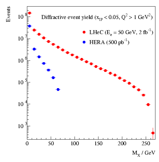
Large improvements in DPDFs are likely to be possible from NLO DGLAP fits to LHeC diffractive structure function data. In addition to the extended phase space in , the extension of the kinematic range towards larger increases the lever-arm for extracting the diffractive gluon density and opens the possibility of significant weak gauge boson exchange, which would allow a quark flavour decomposition for the first time.
Proton vertex factorisation can be tested precisely by comparing the and dependences at the LHeC at different small values in their considerable regions of overlap. The production of dijets or heavy quarks as components of the diffractive system will allow precise testing of QCD collinear factorisation. These processes are driven by boson-gluon fusion () and thus provide complementary sensitivity to the diffractive gluon density to be compared with that from the scaling violations of the inclusive diffractive cross section.
Diffractive final states containing charm signatures or relatively high transverse momentum dijets have been analysed in detail at HERA. In the DIS regime, the cross sections for these processes are reproduced within uncertainties by calculations based on NLO DPDFs extracted from inclusive diffractive data for both the dijet [436, 439, 440, 441] and charm [442, 443] cases. By far the limiting factor in the precision of these tests is the large scale uncertainty on the theoretical predictions, due to the strong kinematic limitations on the accessible jet transverse energies in diffraction at HERA. The situation from HERA photoproduction data is more complex and is usually divided into direct and resolved photon contributions (figures 4.42a and 4.42b, respectively). In the direct photon case, where the highly virtual photon has a point-like coupling, the process is driven by photon-gluon fusion and at the current level of precision, cross sections are well predicted using DPDFs extracted in fits to inclusive diffractive data [440, 377, 444]. In contrast, the resolved photon case introduces sensitivity to the rich partonic structure of the quasi-real photon. It is these partons which participate in the hard scattering sub-process producing the dijets, in a manner which resembles the situation in hadron-hadron scattering. In this case, the possibility of additional rescatterings between the hadronic remnants leads to a non-unit ‘survival probability’ for the rapidity gap [445, 446, 447] and a breakdown of factorisation. Factorisation tests have been carried out on several occasions in diffractive dijet photoproduction at HERA, resulting in a somewhat confused situation on the size of the gap destruction effects [377, 444] and the roles of resolved and direct contributions. Data in which the parton entering the hard scattering carries a lower fraction of the photon momentum are required to clarify the situation, both experimentally and theoretically.
At the LHeC, much larger diffractive jet transverse momenta are measurable () in both photoproduction and DIS. An example study is shown in Fig. 4.43, where the diffractive DIS dijet cross section is simulated for the LHeC kinematics and acceptance, using NLOJET++ [448], with the H1 2006 Fit B DPDFs [434]. Kinematic cuts of , , and , matching the expected LHeC detector geometry and ensuring good containment for the jets and the scattered electron. Jets were reconstructed using the algorithm with and an integrated luminosity of is assumed. The statistical precision remains excellent up to jet values of around , with measurements possible up to around . Theory scale variations in the range of lead to much smaller uncertainties than is the case in the HERA data.
Diffractive dijet photoproduction at the LHeC is expected to be dominated by the resolved photon contribution. A range of transverse momenta similar to the DIS case is accessible in photoproduction, assuming tagging of electrons scattered through small angles as described in Section 3.8. Fractional DPDF momenta , and in the resolved photoproduction case, values, between one and two orders of magnitude smaller than at HERA are typically accessible. All of these improvements will lead to a new level of precision in tests of factorisation and constraints on the diffractive gluon density in new kinematic regions from diffractive jet production at the LHeC [449].
The simulated measurement of the longitudinal proton structure function, described in Section 3.1.5, could also be extended to extract the diffractive analogue, . At small , where the cross section for longitudinally polarised photons is expected to be dominated by a leading twist contribution, an measurement provides further complementary constraints on the role of gluons in the diffractive PDFs. As , a higher twist contribution from longitudinally polarised photons, closely related to that driving vector meson electroproduction, dominates the diffractive cross section in many models [450] and a measurement to even modest precision would give considerable insight. A first measurement of this quantity has recently been reported by the H1 Collaboration [451], though the precision is strongly limited by statistical uncertainties. The LHeC provides the opportunity to explore it in much finer detail.
In contrast to leading proton production, the production of leading neutrons in DIS () requires the exchange of a net isovector system. Data from HERA have supported the view that this process is driven dominantly by charged pion exchange over a wide range of neutron energies [452]. With the planned emphasis on zero degree calorimetry for leading neutron measurements (see Chapter 13), LHeC data will thus constrain the structure of the pion at much lower and larger values than has been possible hitherto. Note also that the combination of rapidity gap detection and zero degree calorimetry offers the possibility of disentangling coherent from incoherent nuclear diffraction.
Diffractive DIS, dipole models and sensitivity to non-linear effects
Diffractive DIS at the LHeC will provide an opportunity to test the predictions of collinear factorisation and the possible onset of non-linear or higher-twist effects in the evolution. Of particular importance is the semi-hard regime GeV2 and as small as possible. It is possible that the non-linear saturation regime will be easier to reach with diffractive than with inclusive measurements, since diffractive processes are mostly sensitive to quantum fluctuations in the proton wave function that have a virtuality of order of the saturation scale , instead of . As a result, power corrections (not the generic corrections, but rather the sub-class of them of order ) are expected to come into play starting from a higher value of in diffractive than in inclusive DIS. Indeed, there is already a hint of this at HERA: collinear factorisation starts to fail below about 3 GeV2 in the case of [38], while it breaks down already around 8 GeV2 in the case of [434]. This fact can alternatively be observed in the feature that models which in principle should only work for small , can in practice be used up to larger for diffractive than for inclusive observables (see e.g. [231]).
With the sort of measurement precision for achievable at the LHeC, it ought to be possible to distinguish between different models, as illustrated in Fig. 4.44. For the simulated data shown here, a conservative situation is assumed, in which the electron beam energy is and only the rapidity gap selection method is used, such that the highest bin is at . H1 Fit B [434] extrapolations (as in Fig. 4.39) are compared with the “b-sat” [276, 277] and bCGC [453] dipole models. As has been found to be necessary to describe HERA data, photon fluctuations to states are included in addition to the usual dipoles used to describe inclusive and vector meson cross sections. Both dipole models differ substantially from the H1 Fit B extrapolation. The LHeC simulated precision and kinematic range are sufficient to distinguish between a range of models with and without saturation effects, and also between different models which incorporate saturation.
Predicting nuclear shadowing from inclusive diffraction in ep
The connection between nuclear shadowing and diffraction was established a long time ago by Gribov [230]. Its key approximation is that the nucleus can be described as a dilute system of nucleons in the nucleus rest frame. The accuracy of this approximation for hadron-nucleus interactions is on the level of a few %, which reflects the small admixture of non-nucleonic degrees of freedom in nuclei and the small off-shellness of the nucleons in nuclei as compared to the soft strong interaction scale. Gribov’s result can be derived using the AGK cutting rules [454] and hence it is a manifestation of unitarity [455, 456]. The formalism can be used to calculate directly cross sections of -nucleus scattering for the interaction with nucleons, but has to be supplemented by additional considerations to account for the contribution of the interactions with nucleons.
In this context, nuclear PDFs at small can be calculated [455, 456] combining unitarity relations for different cuts of the shadowing diagrams corresponding to diffractive and inelastic final states, with the QCD factorisation theorem for hard diffraction [253]. A model-independent expression for the nuclear PDF at fixed impact parameter , valid for the case [455], reads:
| (4.24) | |||||
where and are nuclear and nucleon PDFs, are diffractive nucleon PDFs, , is the nuclear matter density, and with the nucleon mass. Eq. (4.24) satisfies the QCD evolution equations to all orders in . Numerical studies indicate that the dominant contribution to the shadowing probed by present experiments - corresponding to not very small - comes from the region of relatively large , for which small- approximations which involve resummation of terms are not important.
In Eq. (4.24), the interaction of different configurations of the hard probe (e.g. , , vector meson resonances,) are encoded in . For the case of more than nucleons, there are two or more intermediate nucleon diffractive states which may be different and thus result in a different interaction between the the virtual photon and the nucleus. Therefore the interaction of the hard probe with nucleons is sensitive to finer details of the diffractive dynamics, namely the interplay between the interactions of the hard probe with nucleons with different cross sections. This (colour) fluctuation effect is analogous to the inelastic shadowing phenomenon for the scattering of hadrons from nuclei, with the important difference that the dispersion of the interaction cross sections for the configurations in the projectile is much smaller in the hadronic case than in DIS.
In order to estimate this effect, one should note that, experimentally, the energy dependence of hard diffraction is close to that observed for soft Pomeron dynamics (the soft Pomeron intercept ) with the hard Pomeron contribution () being a small correction. This fact indicates that hadron-like (aligned jet) configurations [457], evolved via DGLAP evolution to large , dominate hard diffraction in DIS, while point-like configurations give an important, and increasing with , contribution to small- PDFs. This reduces the uncertainties in the treatment of contributions [329, 408]. Calculations show that the difference between two extreme scenarios of colour fluctuations is for and much smaller for lighter nuclei, see the two FGS10 curves in Figs. 4.12 and 4.18. Besides, fluctuations tend to reduce the shadowing somewhat compared with the approximations neglecting them [232, 455, 458, 459] (compare the FGS10 results in Fig. 4.18 left with those labelled AKST). The gluon density is more sensitive to the magnitude of fluctuations than , as can be inferred from Figs. 4.12 and 4.18 right.
Predictions for inclusive diffraction on nuclear targets
Inclusive diffraction was first measured in DIS events in collisions at the HERA collider. LHeC would be the first electron-ion collider machine, and therefore DDIS off nuclei at this machine will be a completely unexplored territory throughout the whole kinematic domain accessed. This implies a huge discovery potential in this field.
Despite this lack of experimental information on DDIS off nuclei, we have expectations, based on our current understanding of QCD, of how it should look. For instance, the theory of nuclear shadowing allows us to construct nuclear diffractive PDFs for large (see the previous item) while, within the Colour Glass Condensate framework, nuclear diffractive structure functions can be predicted at small . Depending on kinematics and the heavy ion species, different patterns of nuclear shadowing or antishadowing are expected as a function of and . This is just one of many examples of what should be checked with an A collider. Others are the impact parameter dependence introduced in the models, or the relation between nuclear shadowing and diffraction in which relies on what we know on DDIS from HERA. Therefore, in the larger kinematic domain accessible at the LHeC there are many things to discover about the structure of nuclei with diffractive measurements.
One of the main issues which needs to be established is whether the collinear, leading twist, factorisation of inclusive diffraction, proved for protons, is applicable for scattering off nuclei, and the region of its applicability. An important question arises as to where the factorisation would break down, i.e. for which values of and , and whether it depends on the mass number, which would provide most important information on the role of the higher twists in different nuclei. A related issue is whether the factorisation of the hadron vertex which is used in the proton case also holds in the nuclear case. In the analysis of the diffractive structure functions, the Regge-type factorisation is usually assumed. This factorisation states that the diffractive structure function is written as a product of the two factors: one of them is the Pomeron structure function that depends on and , and the other is the Pomeron flux factor that is a function of and . The latter one is usually parameterised using a Regge form with a Pomeron intercept being close to, albeit slightly higher than, the value obtained from soft interactions. It is currently unclear whether such factorisation would still hold in the nuclear case, and this is one of the issues that can be tested at the LHeC. Also the range of possible parameters, like the Pomeron intercept, extracted from such analysis, would provide important details on the nuclear dynamics.
Predictions from a variety of models for nuclear coherent diffraction (see comments on the different types of diffractive processes on nuclei in Section 4.2.3), are shown in Figs. 4.45 and 4.46. The chosen models here are FGS10 [408] and KLMV [461, 462]. Both plots show selected LHeC pseudodata for as a function of in bins of and . Statistical and systematic errors are added in quadrature, with systematic errors estimated to be at the level of . The models give very different predictions both in absolute value and in their detailed dependence on and , which cannot be resolved without LHeC data.
Also shown in Fig. 4.47 are predicted diffractive-to-total ratios of the structure function as a function of . It was demonstrated in [257] that the constancy with of this ratio for the proton - approximately shown by HERA data - can be naturally explained in models which include saturation effects, because in the black disk regime the ratio of diffractive-to-total cross sections tends to a constant value. It has been predicted that in the black disk regime this ratio (for coherent diffraction) may grow as large as [463]. In reality, it could be smaller due to the density distribution in impact parameter.
Within the given energy range the models shown in Fig. 4.47 predict a slight variation with energy. Note however the rather substantial difference between predictions coming from the different models as well as the fact that the plot shows the ratio of structure functions for given and and not integrated cross sections. The uncertainty in modelling the impact parameter is one of the main sources of the discrepancies between the models. Precise LHeC data are required for clarifying these aspects.
Finally we note that, if the scattering on a nucleus at small is dominated almost entirely by the so-called black disk regime, then in principle dramatic effects are expected that can be revealed by studying the final states in diffractive events [174]. As demonstrated in [56], the total virtual photon-nucleus cross section in the black disk limit reads simply
| (4.25) |
where is the nuclear radius and the charge renormalisation constant due to hadrons. The coefficient can be computed in terms of the hadronic components of the photon wave function and related to the cross section for the annihilation of electron-positron pairs into hadrons. Since the elastic part (i.e. that due to diffraction) is half the total cross section in this regime, one can obtain from eq. (4.25) a spectrum of the diffractive masses [174] that, in the centre-of-mass of the diffractively produced system, should be the same as in annihilation. A similar analysis for exclusive processes in this limit shows that the exclusive diffractive production cross sections on nuclei (see section 4.2.3) would exhibit a behaviour instead of the behaviour expected from pQCD. This is due to the fact that a factor which comes from the square of the cross section of the interaction of a small dipole with the target disappears in the black disk limit.
4.2.5 Jet and multi-jet observables, parton dynamics and fragmentation
Introduction
Inclusive measurements provide essential information about the integrated distributions of partons in a proton. However, as was discussed in previous sections, more exclusive measurements are needed to pin down the essential details of the small- dynamics. For example, a central prediction of the BFKL framework at small is the diffusion of the transverse momenta of the emitted partons between the photon and the proton. In the standard collinear approach with integrated parton densities the information about the transverse momentum is not accessible. However, it can be recovered within a different framework which utilises unintegrated parton distribution functions, dependent on parton transverse momentum as well as and . Unintegrated PDFs are natural in the BFKL approach to small- physics. A general, fundamental expectation is that as decreases, the distribution in transverse momentum of the emitted partons broadens, resulting in diffusion.
The specific parton dynamics can be tested by a number of exclusive measurements. These in turn can provide valuable information about the distribution of transverse momentum in the proton. As discussed in [464], for many inclusive observables the collinear approximation with integrated PDFs is completely insufficient, and even just including parton transverse momentum effects by hand may not be sufficient to describe many observables. In DIS, for example, processes needing unintegrated distributions include the transverse momentum distribution of heavy quarks. Similar problems are encountered in hadron collisions when studying heavy quark and Higgs production. The natural framework using unintegrated PDFs gives a much more reliable description. Furthermore, lowest-order calculations in the framework with unintegrated PDFs provide a much more realistic description of cross sections concerning kinematics. This may well lead to NLO and higher corrections being much smaller numerically than they typically are at present in standard collinear factorisation, since the LO description is better.
This approach, however, calls for precise measurements of a variety of relatively exclusive processes in a wide kinematic range. As discussed below, measurements of dijets, forward jets and particles, as well as transverse energy flow, are required to constrain the unintegrated PDFs and will give valuable information about parton dynamics at small . While we will discuss the case of DIS on a proton, all conclusions can be paralleled for DIS on nuclei.
Unintegrated PDFs
The standard integrated parton densities are functions of the longitudinal momentum fraction of a parton relative to its parent hadron, with an integral over the parton transverse momentum. In contrast, unintegrated, or transverse-momentum-dependent (TMD), parton densities depend on both parton longitudinal momentum fraction and parton transverse momentum. Processes for which unintegrated densities are natural include the Drell-Yan process (and its generalisation to Higgs production), and semi-inclusive DIS (SIDIS). In SIDIS, we need TMD fragmentation functions as well as TMD parton densities.
In the literature there are several apparently different approaches to TMD parton densities, with varying degrees of explicitness in the definitions and derivations.
- •
- •
- •
Central to this subject is the concrete definition of TMD densities, and complications arise because QCD is a gauge theory. A natural initial definition uses light-front quantisation: the unintegrated density of parton in hadron would be
| (4.26) |
where and are light-front annihilation and creation operators, and label parton flavor and helicity, while is its momentum, and only connected graphs ‘c’ are considered. The ‘?’ over the equality sign warns that the formula does not apply literally in QCD. Expressing and in terms of fields gives the TMD density as the Fourier transform of a light-front parton correlator. For example, for a quark
| (4.27) |
One can similarly define a TMD fragmentation function [466] , for the probability density of final-state hadron in an outgoing parton .
The corresponding factorisation formula for SIDIS is [469]
| (4.28) |
where and are the fractional longitudinal momentum and the transverse momentum of the detected hadron relative to the simplest parton-model calculation of the outgoing jet, while is the hard-scattering factor for electron-quark elastic scattering; see Fig. 4.48(a). In the fragmentation function in Eq. (4.28), the use of with its factor of is because the transverse-momentum argument of the fragmentation function is a transverse momentum of the outgoing hadron relative to the parton initiating the jet, whereas is the transverse momentum of a parton relative to a hadron.
| (a) | (b) |
|---|
The most obvious way of applying (4.27) in QCD is to define the operators in light-cone gauge , or, equivalently, to attach Wilson lines to the quark fields with a light-like direction for the Wilson lines. One minor problem in QCD is that, because the wave function is infinite (see below), the exact probability interpretation of parton densities cannot be maintained.
A much harder problem occurs because QCD is a gauge theory. Evaluating TMD densities defined by (4.27) in light-cone gauge gives divergences where internal gluons have infinite negative rapidity [465]. These cancel only in the integrated density. The physical problem is that any coloured parton entering (or leaving) the hard scattering is accompanied by a cloud of soft gluons, and the soft gluons of a given transverse momentum are distributed uniformly in rapidity. A parton density defined in light-cone gauge corresponds to the asymptotic situation of infinite available rapidity.
A quark in a realisable hard scattering can be considered as having a transverse recoil against the soft gluons, but with a physically restricted range of rapidity. So a proper definition of a TMD density must implement a rapidity cut-off in the gluon momenta. Evolution equations must take into account the rapidity cut-off. The CSS formalism [465] has an explicit form of the rapidity cut-off and an equation for the dependence of TMD functions on the cut-off. But in any alternative formalism the need in the definitions for a cut-off to avoid rapidity divergences is non-negotiable.
Parton densities and fragmentation functions are only useful because they appear in factorisation theorems, so a useful definition must allow useful factorisation theorems to be formulated and derived. An improved definition involving Wilson line operators has recently been given in [475]; see also [476].
A second train of argument leads to a related kind of factorisation (the so-called -factorisation) for processes at small [140]. A classic process is photo- or electro-production of charm pairs , for which -factorisation has the form
| (4.29) |
see Fig. 4.48(b). Here , and is the mass of the heavy quark. The corresponding definition of the TMD gluon density [470] is said to use light-cone gauge, but there is in fact a hidden rapidity cut-off resulting from the use of the BFKL formalism.
Although both (4.28) and (4.29) use -dependent parton densities, there are important differences. In (4.29), the hard scattering cross section has the incoming gluon off-shell, whereas in (4.28), the hard scattering uses on-shell partons. This is associated with a substantial difference in the kinematics. In (4.28) for SIDIS, the transverse momenta of the partons relative to their hadrons are less than , which allows the neglect of parton virtuality in the hard scattering. This approximation fails at large partonic transverse momentum, , but ordinary collinear factorisation is valid in that region. So the factorisation formula is readily corrected, by adding a suitable matching term [465].
In contrast, in the small- formula (4.29), the gluon transverse momentum is comparable with the hard scale . So it is not appropriate to neglect with respect to , and the hard scattering is computed with an off-shell gluon. Factorisation is actually obtained from BFKL physics, where the gluons in Fig. 4.48(b) couple the charm quark subgraph to a subgraph where the lines have much larger rapidity.
The evolution equation of the CS-style TMD functions used in (4.28) gives the dependence of the TMD functions on the rapidity difference between the hadron and the virtual photon momenta. The results for TMD functions and for the cross sections can finally be obtained [469] in terms of (a) ordinary integrated parton densities and fragmentation functions, (b) perturbatively calculable quantities, and (c) a restricted set of non-perturbative quantities. The most important of these non-perturbative quantities is the distribution in recoil transverse momentum per unit rapidity against the emission of the soft interacting gluons, which is exponentiated after evolution. Importantly, it is independent of and , and it is universal between processes [477], and different only between gluons (colour octet) and quarks (colour triplet). There is also what can be characterised as a non-perturbative intrinsic transverse momentum distribution in both parton densities and fragmentation functions. In the quark sector, all but the fragmentation function are well measured in Drell-Yan processes [478].
On the other hand, evolution for the small- formalism in (4.29) is given by the BFKL method.
The avenues for further improvement on this subject are both theoretical and experimental. On the theory side, these concern the relation between different formalisms for evolution [465, 469, 246, 474, 479], the extension of factorisation theorems to a larger number of particles in the final state, and the matching to Monte Carlo generators. On the experimental side, the sensitivity to TMD functions is linked to a sensitivity to parton transverse momentum. This is the case of SIDIS at low transverse momentum. Another interesting process which would enable the TMD gluon functions to be probed is , with the pions being in different directions (different jets), but such that they are close to back-to-back in the (the so-called brick wall) frame.
Finally, measuring SIDIS and dijet production off protons or nuclei at the LHeC will allow detailed investigations of non-linear parton evolution in QCD. In this respect, the SIDIS cross section [480] and dihadron production [481] have been studied in the CGC framework. It turns out that, for small , one is sensitive to the saturation regime of the target (proton or nucleus) wave function if the transverse momentum of the produced hadron is of the order of the saturation momentum.
Dijet production and angular decorrelation
Dijet production in high energy deep inelastic electron-proton scattering is a very valuable process for the study of the small- behaviour in QCD. The dominant process is illustrated in Fig. 4.49, which is that of the dijet production. The incoming gluon can have sizeable transverse momentum accumulated from diffusion in along the gluon chain. As Bjorken- becomes smaller, and therefore the longitudinal momentum of the gluon also decreases, larger values of the transverse momentum can be sampled. This will lead to an azimuthal decorrelation between the jets which increases with decreasing . The definition of is indicated in Fig. 4.49. That is, the jets are no longer back-to-back since they must balance the sizeable transverse momentum of the incoming virtual gluon.
This picture of dijet production is to be contrasted with the conventional picture which uses integrated parton distributions, and typically leads to a narrow distribution about the back-to-back jet configuration. Higher orders usually broaden the distribution. However, as shown by direct measurements of DIS dijet data [482], NLO DGLAP calculations are not able to accommodate the pronounced effect of the decorrelation.
Explicit calculations for HERA kinematics show that the models which include the resummation of powers of compare favourably with the experimental data [483, 484, 485, 486, 487]. The proposal and calculations to extend such studies to diffractive DIS also exist [488, 489].
In Fig. 4.50 we show the differential cross section as a function of for jets in the region with GeV and GeV found with the jet algorithm in the kinematic range GeV, for different regions in . The ‘MEPS’ prediction comes from a Monte Carlo generator [147] using matrix elements with a DGLAP-type parton shower. The ‘CDM’ prediction uses the same generator [147], but with higher order parton radiation simulated with the Colour Dipole Model [490], thus effectively including some diffusion. Finally, the CASCADE Monte Carlo prediction [491], uses off-shell matrix elements convoluted with an unintegrated gluon distribution (CCFM set A), with subsequent parton showering according to the CCFM evolution equation.
At large all predictions agree reasonably well, in both shape and normalisation. At smaller the -distribution becomes flatter for CDM and CASCADE, indicating higher order effects leading to a larger decorrelation of the produced jets. Whereas a decorrelation is observed, its size depends on the details of the parton evolution and thus a measurement of the cross section provides a direct measurement of higher order effects which need to be taken into account at small .
Thus, in principle, a measurement of the azimuthal dijet distribution offers a direct determination of the -dependence of the unintegrated gluon distribution. When additionally supplemented by inclusive measurements, it can serve as an important constraint for the precise determination of the fully unintegrated parton distribution, with the transverse momentum dynamics in the proton completely unfolded.
Dihadron correlations
Another interesting observable which is directly sensitive to the transverse momentum dependence of the parton distribution in the proton or nucleus is the process of two hadron production1212 12 This observable is currently discussed in the forward (proton) rapidity region in dAu collisions at RHIC and it shows features suggestive of physics beyond standard collinear factorisation, although no consensus has been reached so far, see [310, 311, 312, 313, 314] and references therein.. Instead of two jets, one observes semi-inclusively two hadrons with certain transverse momentum. One can define the function which describes the angular correlation of the two produced hadrons in the following way:
| (4.30) |
In the above formula are the longitudinal momentum fractions of the two produced hadrons w.r.t. the photon momentum and is the azimuthal angle between them. The quantity is the single inclusive cross section. In Fig. 4.51 we show the results of the calculation using the formalism presented in [480]. The gluon density was evaluated using the GBW model [256] for the proton and a modified version of the same model for the nucleus. The electron energy is assumed to be GeV, the proton energy is and the nucleus energy is . Also for the direct comparison with the nuclear case the curve with proton energy of is shown. The transverse momenta of the produced pions are integrated over, it is assumed that the leading particle has a minimum transverse momentum of and the associated particle . The photon virtuality is , and the fractions of the longitudinal momenta of the produced pions are fixed to be equal to . One clearly sees that the correlation function is wider for a larger target (nucleus) than for the proton. This suppression of the peak in the correlation function can be interpreted in this model as the effect of the stronger saturation in the gluon density for the nucleus than for the proton. We also see that the correlation function varies mildly with the available energy for the same target (i.e. proton). One observes stronger de-correlation of the produced hadrons with a higher energy or at smaller values of which is indicative of the importance of the effects for this observable. Therefore the measurement of the dihadron correlation provides another way of constraining the unintegrated gluon distribution. In particular, measuring the dihadron correlations in DIS provides with a unique opportunity[481, 492] to directly study the so-called Weizsäcker-Williams unintegrated gluon distribution.
Forward observables
It was proposed some time ago [493, 494] that a process which would be very sensitive to the parton dynamics and the transverse momentum distribution was the production of forward jets in DIS. According to [493, 494], DIS events containing identified forward jets provide a particularly clean window on small- dynamics. The schematic view of the process is illustrated in Fig. 4.52. The forward jet transverse momentum provides the second hard scale . Hence one has a process with two hard scales: the photon virtuality and the transverse momentum of the forward jet . As a result the collinear (DGLAP) configurations (with no diffusion and strongly ordered transverse momenta) can be eliminated by choosing the scales to be of comparable size, . Additionally, the jet is required to be produced in the forward direction by demanding that , the longitudinal momentum fraction of the produced jet, is as large as possible, and is as small as possible. This requirement selects events with a large sub-energy between the jet and the virtual photon, such that the BFKL framework should be applicable. There have been dedicated measurements of forward jets at HERA [495, 496, 497, 498, 499, 500], which demonstrated that DGLAP dynamics at NLO are indeed incompatible with the experimental measurements. On the other hand, calculations based on resummations of powers of (BFKL and others) [501, 502, 503, 504, 505, 506, 507] are consistent with the data. The azimuthal dependence of forward jet production has also been studied [508, 509] as a sensitive probe of the small- dynamics.
Another observable that provides a valuable insight into the features of small- physics is the transverse energy (-flow) accompanying DIS events at small . The diffusion of the transverse momenta in this region leads to a strongly enhanced distribution of at small . As shown in [510, 511], small- evolution results in a broad Gaussian -distribution as a function of rapidity. This should be contrasted with the much smaller -flow obtained assuming strong -ordering as in DGLAP-based approaches, which give an -distribution that narrows with decreasing , for fixed .
The first experimental measurements of the -flow in small- DIS events indicate that there is significantly more than is given by conventional QCD cascade models based on DGLAP evolution. Instead we find that they are in much better agreement with estimates which incorporate dynamics beyond fixed-order DGLAP [512, 490, 506] such as BFKL evolution. The latter dynamics are characterised by an increase of the -flow in the central region with decreasing .
However, the experimental data from HERA do not enable a detailed analysis due to their constrained kinematics. At the LHeC one could perform measurements with large separations in rapidity and for different selections of the scales . In particular, there is a possibility of varying scales to test systematically the parton dynamics from the collinear (strongly ordered) regime to the BFKL (equal scale, Regge kinematics) regime . Measurements of the energy flow in different -intervals, in the small- regime, should therefore allow a definitive check of the applicability of BFKL dynamics and of the eventual presence of more involved, non-linear effects.
A simulation of forward jet production at the LHeC is shown in Figs. 4.53 and 4.54. The jets are required to have GeV with a polar angle or in the laboratory frame. Jets are found with the SISCone jet-algorithm [513]. The DIS phase space is defined by GeV, .
In Fig. 4.53 the differential cross section is shown as a function of Bjorken for an electron energy of GeV. The calculations are obtained from the MEPS [147], CDM [490] and CASCADE [506] Monte Carlo models, as described in the previous section. Predictions for and are shown. One can clearly see that the small- range is explored in detail with the small angle scenario. In Fig. 4.54 the forward jet cross section is shown when using instead of (Fig. 4.53). It is important to note that good forward acceptance of the detector is crucial for the measurement of forward jets. The dependence of the cross section on the acceptance angle is very strong as is evident from comparisons between the cross sections for different cuts in Figs. 4.53 and 4.54.
A complementary reaction to that of forward jets is the production of forward mesons in DIS. Despite having a lower rate, this process offers some advantages over forward jet production. By looking onto single particle production the dependencies on the jet finding algorithms can be eliminated. Also, the non-perturbative hadronisation effects can be effectively encompassed into fragmentation functions [502].
Perturbative and non-perturbative aspects of final state radiation and hadronisation
The mechanism through which a highly virtual parton produced in a hard scattering gets rid of its virtuality and colour and finally projects onto an observable final state hadron, is unknown to a great extent (see [337] and references therein). The different postulated stages of the process are illustrated in Fig. 4.55. The coloured parton undergoes QCD radiation before forming first a coloured excited bound state (pre-hadron), then a colourless pre-hadron and ultimately a final state hadron. These sub-processes are characterised by different time scales. While the first stage can be described in perturbative QCD [514], subsequent ones require models (e.g. the QCD dipole model for the pre-hadron stages) and non-perturbative information.
The LHeC offers great opportunities to study these aspects and improve our understanding of all of them. The energy of the parton which is struck by the virtual photon implies a Lorentz dilation of the time scales for each stage of the radiation and hadronisation processes. All of them are influenced by the fact that they do not take place in the vacuum, but within the QCD field created by the other components of the hadron or nucleus. While at fixed target SIDIS or DY experiments, the lever arm in energy is relatively small (energy transfer to the struck parton in its rest frame GeV), at the LHeC this lever arm will be huge ( GeV; see also in Subsec. 3.7.2 the abundant yield of expected high transverse momentum jets in photoproduction), implying that the different stages can be considered to happen in or out of the hadron field depending on the parton energy. Furthermore, the fact that we can introduce a piece of coloured matter of known length and density - a nucleus - by doing Pb collisions at different centralities, allows a controllable variation of the contribution of the different processes. The induced differences in the final distributions of hadrons, both in terms of their momenta and of their relative abundance, will provide important information about the time scales and the detailed physical mechanisms at work in each stage. Dramatic effects are predicted in some models [174], with a significant suppression of the forward hadron spectra due to the existence of a dense partonic system. Note that SIDIS experiments already provide information for the determination of standard fragmentation functions (see [515, 516] for a recent analysis). The other pieces of information, coming mainly from experiments, will not be improved until next-generation linear colliders become available.
Furthermore, these studies will shed light on two aspects already discussed in Subsec. 4.1.4, related to the study of ultra-relativistic heavy-ion collisions: the characterisation of the medium created in such collisions through hard probes, and the details of particle production in a dense situation which will define the initial conditions for the collective behaviour of this medium. Concerning the latter, our theoretical tools for computing particle production in A collisions are more advanced e.g. within the CGC framework, and on a safer ground than in nucleus-nucleus collisions (see Subsec. 4.1.1 and e.g. [336] and refs. therein). The possibility of disentangling the different mechanisms through which the factorisation that is used in dilute systems - collinear factorisation [209] - becomes broken by density effects (e.g. initial and final state energy loss or final state absorption) will be possible at the LHeC and will complement existing studies done at much smaller energies in fixed target SIDIS and DY experiments [337].
In order to quantify the possibilities for SIDIS studies, we first show the expected cross sections for production in and Pb collisions at the LHeC for GeV, see Fig. 4.56. There the calculations are done at NLO [517], using as nucleon PDFs those from [282] and, in order to illustrate their effect, different nuclear PDFs [326, 167] and both ordinary [515, 516] and modified [518]1313 13 In this reference, fragmentation functions in nuclear matter are extracted in a DGLAP analysis at LO and NLO. fragmentation functions. Cuts have been applied as in the H1 study [519]1414 14 Studies with looser cuts - a more realistic situation at the LHeC, and of the achievable resolution in and , are left for the future. whose data are well reproduced by the NLO calculation: angle of the from the proton in the laboratory , pion energy fraction and pion transverse momentum GeV/c. All scales in the calculation have been fixed to (-factors and the scale dependence of the results are discussed in [517]). From the plots in the figure, it becomes clear that even for these very restrictive cuts and for a modest integrated luminosity of 1 fb-1, a large number of pions will be produced with relatively large transverse momentum. The nuclear effects on PDFs and on fragmentation require measurements with good statistic and systematic precision in order to be disentangled.
The results with looser cuts: , that could be achieved at the LHeC, have also been studied. Their effect is an increase of the cross section by a factor with respect to the results with the more restrictive H1 cuts.
SIDIS also offers the possibility to measure the nuclear effects on fragmentation functions through the double ratio for nucleus and particle :
| (4.31) |
with the number of scattered electrons at a given and i.e. the DIS cross section. At LO and for a single quark flavour, this double ratio becomes the ratio of fragmentation functions in A over , see [337]. Usually, the energy of the lepton-hadron/nucleus collisions are the same in numerator and denominator, and the collisions in the denominator are D in order to suppress isospin effects as much as possible.
In order to estimate the nuclear modifications of fragmentation functions for the case of the LHeC, we compute this double ratio. For the numerator, we consider Pb collisions at 60+2750 GeV while for the denominator we take collisions at 60+7000 GeV. We follow the model in [520] which considers the energy loss of the parent parton though radiative processes1515 15 For this, we use the quenching weights in [521] instead of the simplified expressions employed in [520]. plus formation time arguments which make the effective length of traversed nuclear matter smaller at small than the geometrical one . We use the LO nucleon PDFs in [282] and the nucleon fragmentation functions in [515, 516], and also considered the nuclear modification of PDFs in [167]. We employ a value of the transport coefficient characterising the strength of the interaction of a quark with nuclear matter GeV2/fm 1616 16 This value is larger than the one used in [520]. We have checked that the model reproduces fixed target data on the dependence of the ratio (4.31) for pion production on Kr over D in [522] using this value of without formation time considerations..
The results for production are shown in Fig. 4.57. Several conclusions can be drawn. First, the effect of the difference in energy between numerator and denominator, and of isospin, are very small. Second, nuclear effects on fragmentation are larger for smaller , as expected in a model in which the energy loss becomes energy-independent [520, 521]. Third, the nuclear suppression is larger for larger and it decreases with increasing , both effects due to the steepness of the fragmentation function and its evolution with . Finally, formation time limitations are only sizeable for small , as naively expected due to the possibility of hadron formation inside the nucleus in this kinematic region, see [520].
From these results we conclude that the study of SIDIS at the LHeC looks very promising. Still, extensive analyses at detector level are required in order to establish the accessible kinematic regions and to further explore the possibilities for particle identification.
4.2.6 Implications for ultra-high energy neutrino interactions and detection
The stringent constraints of the parton distributions at very small from a future LHeC will have important implications for neutrino astronomy. Ultra-high energy neutrinos can provide important information about distant astronomical objects and the origin of the Universe. They have attracted a lot of attention during recent years, see the reviews [523, 524]. Neutrino astronomy has many advantages over conventional photon astronomy. This is due to the fact that neutrinos, unlike photons, interact only weakly, so they can travel long distances being practically undisturbed. The typical interaction lengths for neutrinos and photons at energy are about
Thus, very energetic photons with energy bigger than cannot reach the Earth from the very distant corners of our Universe without being rescattered. In contrast, neutrinos can travel very long distances without interacting. They are also not deflected by galactic magnetic fields, and therefore at ultra-high energies the angular distortion of the neutrino trajectory is very small. As a result, highly energetic neutrinos reliably point back to their sources. The interest in the neutrinos at these high energies has led to the development of several neutrino observatories, see [524] and references therein.
For reliable observations based on neutrino detection, precise knowledge about their production rates and interactions is essential to estimate the background, the expected fluxes and the detection probabilities. Even though neutrinos interact only weakly with other particles, strong interactions play an essential role in the calculations of their production rates and interaction cross sections. This is due to the fact that neutrinos are produced in the decays of various mesons such as and even , which are produced in high-energy proton-proton (or proton-nucleus or nucleus-nucleus) collisions. These hadronic processes occur mainly in the atmosphere though possibly also in the accretion discs of remote Active Galactic Nuclei. Further, the interactions of highly energetic neutrinos with matter are dominated by the deep inelastic cross section with nucleons or nuclei. Hence, low- information from high-energy collider experiments such as HERA, Tevatron, LHC and, most importantly, the future LHeC, is invaluable.
One of the main uncertainties (if not the dominant one) in the current limits on high-energy neutrino production is due to the neutrino-nucleon (nucleus) cross section. In fact, event rates are proportional to the neutrino cross section in many experiments. This cross section involves the gluon distribution probed at very small values of Bjorken , down to even , which corresponds to a very high centre of mass energy.
To visualise the kinematic regime probed in ultra-high energy neutrino-nucleon interactions, contour plots of the differential cross section in the plane are shown in Fig. 4.58. The contours enclose regions with different contributions to the total cross section . For very high energy the dominant contribution comes from the domain and where is the nucleon mass, inaccessible to any current or proposed accelerators. However, at lower neutrino energy the relevant domain of could be very well covered by the LHeC, thus providing important new constraints on the neutrino-nucleon cross section.
On the other hand, another process that has been proposed for neutrino detection comes from the discovery of neutrino flavor oscillations, which makes it possible that high rates of neutrinos reach the Earth despite being heavily suppressed in most postulated production mechanisms. The possibility to search for ’s by looking for leptons that exit the Earth, Earth-skimming neutrinos, has been shown to be particularly advantageous to detect neutrinos of energies in the EeV () range [525]. The short lifetime of a lepton originating a neutrino charged current interaction allows the to decay in flight while still close to the Earth’s surface, producing an outgoing air shower, detectable in principle by various techniques. This channel suffers from negligible contamination for other neutrino flavors. The sensitivity to ’s through the Earth-skimming channel directly depends both on the neutrino charged current cross section and on the range (the energy loss) which is determined by the amount of matter with which the neutrino has to interact to produce an emerging . It turns out that the energy loss is also determined by the behaviour of the proton and nucleus structure functions at very small values of , see e.g. [526]. The average energy loss per unit depth, , is conveniently represented by:
| (4.32) |
where the term is due to ionisation, is the sum of fractional losses due to pair production, bremsstrahlung and photo-nuclear interactions, is Avogadro’s number and is the mass number. The parameter is nearly constant and the term dominates the energy loss above a critical energy that for leptons is a few TeV, with the photo-nuclear interaction being dominant for energies exceeding GeV (as already assumed in Eq. (4.32)). In Fig. 4.59 the relative contribution to of different and regions is shown. It can be observed that the energy loss is dominated by very small and, in contrast to the case of the neutrino cross section, by small and moderate .
As the LHeC will be able to explore a new regime of low and moderate-to-high , and constrain the parton distributions, the measurements performed at this collider will be invaluable for the precise evaluation of the neutrino-nucleon (or nucleus) scattering cross sections and energy loss necessary for ultra-high energy neutrino astronomy.
Chapter 5 New Physics at High Energy
The LHC is the primary machine to search for physics beyond the Standard Model at the TeV energy scale. The role of the LHeC, which is projected to operate when the LHC begins its high luminosity phase, is to complement and possibly resolve the observation of new phenomena based on the specifics of deep inelastic scattering at energies extending to beyond a TeV. At the LHC, it will not always be possible to measure with precision the parameters of the new physics. In this section, it is shown that in several cases the LHeC can probe in detail deviations from the expected electroweak interactions shared by leptons and quarks, thus adding essential information on the new physics. Previous studies [527, 2, 528, 529] of the potential of high-energy colliders for the discovery of exotic phenomena have considered a number of processes, most of which are reviewed here. At the time this report is completed, the only sign for new physics at the LHC, apart from new quark states and a plethora of more and more stringent limits on the mass of new particles and their existence, higher symmetries or extra dimensions, consists in the still tentative observation of a new state at about GeV mass, which may be associated to the long searched for SM Higgs boson. This section therefore concludes with a study of the Higgs production at the LHeC in the rather clean channel.
5.1 New physics in inclusive DIS at high
The LHeC collider would enable the study of deep inelastic neutral current scattering at very high squared momentum transfers, , thus probing the structure of electron-quark () interactions at very short distances. At these small scales new phenomena not directly detectable may yet become observable as deviations from the Standard Model predictions. A convenient tool to assess the experimental sensitivity beyond the maximal available centre of mass energy and to parameterise indirect signatures of new physics is the concept of an effective four-fermion contact interaction. If the contact terms originate from a model where fermions have a substructure, a compositeness scale can be related to the size of the composite object. If they are due to the exchange of a new heavy particle, such as a leptoquark, the effective scale is related to the mass and coupling of the exchanged boson. Contact interaction phenomena are best observed as a modification of the expected dependence and all information is essentially contained in the differential cross section . An alternative way to parameterise the effects of fermion substructure makes use of form factors, which would also lead to deviations of with respect to the SM prediction. As a last example, low scale quantum gravity effects, which may be mediated via gravitons coupling to SM particles and propagating into large extra spatial dimensions, could also be observed as a modification of at highest . These possible manifestations of new physics in inclusive DIS are addressed in this section.
5.1.1 Quark substructure
The remarkable similarities in the electromagnetic and weak interactions of leptons and quarks in the Standard Model, and their anomaly cancellations in the family structure, strongly suggest a fundamental connection. It would therefore be natural to conjecture that they could be composed of more fundamental constituents, or that they form a representation of a larger gauge symmetry group than that of the Standard Model, in a Grand Unified Theory.
A possible method to investigate fermion substructures is to assign a finite size of radius to the electroweak charges of leptons and/or quarks while treating the gauge bosons and still as point-like particles [530]. A convenient parameterisation is to introduce ‘classical’ form factors at the gauge boson–fermion vertices, which are expected to diminish the Standard Model cross section at high momentum transfer:
| (5.1) | |||||
| (5.2) |
The form factor is related to the Fourier transform of the electroweak charge distribution within the fermion. The square root of the mean-square radius of this distribution, , is taken as a measure of the particle size. Since the point-like nature of the electron/positron is already established down to extremely low distances in and experiments, only the quarks are allowed to be extended objects, i.e. the form factor can be set to unity in the above equation.
Figure.5.1 shows the sensitivity that the LHeC could reach on the “quark radius” [531]. Two beam energy configurations have been studied ( GeV and GeV), and two values of the integrated luminosity, per charge, have been assumed in each case. A sensitivity to quark radius below m could be reached, about one order of magnitude better than the current constraints.
At the LHC, quark compositeness can be investigated by studying the properties of dijet events, in particular their mass spectrum together with angular distributions. This is usually done in the context of four-quark contact interactions (CI), defined similarly to the contact interactions that are considered in the next paragraph (see Eq. 5.3 and Eq. 5.4). With the statistics collected in 2011 at TeV, the ATLAS experiment rules out four-quark contact interaction scales lower than TeV [532]. This is not directly related to the quark radius considered above, the latter being defined from the distribution of electroweak charge within the quark. Dijet production at the LHC is largely dominated by strong interactions, and a deviation from the SM of the electroweak production of dijets would lead to a very small effect in the total dijet production cross section. From a naive scaling of the CI contribution by , the current bound would translate into an upper limit of m on the quark radius. With fb-1 of LHC data at TeV, a factor of about could be gained on this sensitivity.
5.1.2 Contact interactions
New currents or heavy bosons may produce indirect effects through the exchange of a virtual particle interfering with the and fields of the Standard Model. For particle masses and scales well above the available energy, , such indirect signatures may be investigated by searching for a four-fermion point-like contact interaction. The most general chiral invariant Lagrangian for neutral current vector-like contact interactions can be written in the form [533, 534, 535]
| (5.3) | |||||
where the indices and denote the left-handed and right-handed fermion helicities and the sum extends over up-type and down-type quarks and antiquarks . In deep inelastic scattering at high the contributions from the first generation and quarks dominate and contact terms arising from sea quarks , and are strongly suppressed. Thus, there are eight independent effective coupling coefficients, four for each quark flavour
| (5.4) |
where and indicate the helicities, is a scale parameter and is often set to , which determines the interference sign with the Standard Model currents. The ansatz eq. (5.3) can be easily applied to any new phenomenon, e.g. compositeness, leptoquarks or new gauge bosons, by an appropriate choice of the coefficients . Scalar and tensor interactions of dimension 6 operators involving helicity flip couplings are strongly suppressed at Hera [535] and therefore not considered.
Figure 5.2 shows the sensitivity that the LHeC could reach on the scale , for two example cases of contact interactions [531]. In general, with fb-1 of data, LHeC would probe scales between and , depending on the model. The ultimate sensitivity of LHC to such interactions, which would affect the di-electron Drell-Yan (DY) spectrum at high masses, is similar. With fb-1 of data at TeV, the ATLAS and CMS experiments rule out contact interactions with a scale below TeV. The sensitivity will extend to typically TeV with fb-1 of data at TeV.
Figure 5.3 shows how the DY cross section at the LHC would deviate from the SM value, for three examples of contact interactions. In the “LL” model considered here, the sum in eq. (5.3) only involves left-handed fermions and all amplitudes have the same phase . With only data, it will be difficult to determine simultaneously the size of the contact interaction scale and the sign of the interference of the new amplitudes with respect to the SM ones: for example, for and , the decrease of the cross section with respect to the SM prediction for di-electron masses below , which is characteristic of a negative interference, is too small to be firmly established when uncertainties due to parton distribution functions are taken into account. Angular distributions and forward-backward asymmetries can help in principle to disentangle between the various possible CI scenarios. However, the statistical uncertainties expected for dilepton masses above TeV limit the power of these variables to scales well below the sensitivity limit. A similar conclusion was reached in [536] in a study of the indirect effects of a very heavy boson on dilepton events at the LHC.
For the same “LL” model, the sign of this interference can be unambiguously determined
at LHeC from the asymmetry of in and data, as shown
in Fig. 5.4.
Moreover, with a polarised lepton beam, collisions would help determine the chiral structure of the new interaction. More generally, it is very likely that both and data would be necessary to underpin the structure of new physics which would manifest itself as an contact interaction. Such a complementarity of , (and also ) data was studied in [537] in the context of the Tevatron, HERA and LEP colliders.
5.1.3 Kaluza-Klein gravitons in extra-dimensions
In some models with large extra dimensions, the SM particles reside on a four-dimensional “brane”, while the spin 2 graviton propagates into the extra spatial dimensions and appears in the four-dimensional world as a tower of massive Kaluza-Klein (KK) states. The summation over the enormous number of Kaluza-Klein states up to the ultraviolet cut-off scale, taken as the Planck scale in the space, leads to effective contact-type interactions between two fermion lines, with a coupling . In scattering, the exchange of such a tower of Kaluza-Klein gravitons would affect the dependence of the DIS cross section . At LHeC, such effects could be observed as long as the scale is below . While at the LHC, virtual graviton exchange may be observed for scales up to , and the direct production of gravitons, for scales up to depending on , would allow this phenomenon to be studied further, LHeC data may determine that the new interaction is universal by establishing that the effect in the cross section is independent of the lepton charge and polarisation, and, to some extent, of the quark flavour.
5.2 Leptoquarks and leptogluons
The high energy of the LHeC extends the kinematic range of DIS physics to much higher values of electron-quark mass , beyond those of HERA. By providing both baryonic and leptonic quantum numbers in the initial state, it is ideally suited to a study of the properties of new bosons possessing couplings to an electron-quark pair in this new mass range. Such particles can be squarks in supersymmetric models with -parity violation (), or first-generation leptoquark (LQ) bosons which appear naturally in various unifying theories beyond the Standard Model (SM) such as: [44], where new fields can mediate interactions between leptons and quarks; extended technicolor [47, 538], where leptoquarks result from bound states of technifermions; the Pati-Salam model [45], where the leptonic quantum number is a fourth colour of the quarks or in lepton-quark compositeness models. They are produced as single channel resonances via the fusion of incoming electrons with quarks in the proton. They are generically referred to as “leptoquarks” in what follows. The case of “leptogluons”, which could be produced in collisions as a fusion between the electron and a gluon, is also addressed at the end of this section.
5.2.1 Phenomenology of leptoquarks in collisions
In collisions, LQs may be produced resonantly up to the kinematic limit of via the fusion of the incident lepton with a quark or antiquark coming from the proton, or exchanged in the channel, as illustrated in Fig. 5.5.
The coupling at the vertex is an unknown parameter of the model.
In the narrow-width approximation, the resonant production cross section is proportional to where is the density of the struck parton in the incoming proton.
The resonant production or -channel exchange of a leptoquark gives or final states leading to individual events indistinguishable from SM NC and CC DIS respectively. For the process , the distribution of the transverse energy of the final state lepton shows a Jacobian peak at , being the LQ mass. Hence the strategy to search for a LQ signal in collisions is to look, among high (i.e. high ) DIS event candidates, for a peak in the invariant mass of the final pair. Moreover, the significance of the LQ signal over the SM DIS background can be enhanced by exploiting the specific angular distribution of the LQ decay products (see spin determination, below).
5.2.2 The Buchmüller-Rückl-Wyler Model
A reasonable phenomenological framework to study first generation LQs is provided by the BRW model [539]. This model is based on the most general Lagrangian that is invariant under , respects lepton and baryon number conservation, and incorporates dimensionless family diagonal couplings of LQs to left- and/or right-handed fermions. Under these assumptions LQs can be classified according to their quantum numbers into 10 different LQ isospin multiplets (5 scalar and 5 vector), half of which carry a vanishing fermion number ( and denoting the baryon and lepton number respectively) and couple to while the other half carry and couple to . These are listed in Table 5.1.
| Prod./Decay | Prod./Decay | ||||
|---|---|---|---|---|---|
| Scalar Leptoquarks | |||||
| Vector Leptoquarks | |||||
We use the nomenclature of [540] to label the different LQ states. In addition to the underlying hypotheses of BRW, we restrict LQs couplings to only one chirality state of the lepton, given that deviations from lepton universality in helicity suppressed pseudoscalar meson decays have not been observed [541, 542].
In the BRW model, LQs decay exclusively into and/or and the branching ratio is fixed by gauge invariance to 0.5 or 1 depending on the LQ type.
5.2.3 Phenomenology of leptoquarks in collisions
Pair production
In collisions leptoquarks would be mainly pair-produced via or interactions. As long as the coupling is not too strong (e.g. or below, corresponding to a strength similar to or lower than that of the electromagnetic coupling, ), the production cross section is essentially independent of . At the LHC, LQ masses up to about (scalar LQs) and (vector LQs) will be probed [543], independently of the coupling . However, the determination of the quantum numbers of a first generation LQ in the pair-production mode is not possible (e.g. for the fermion number) or ambiguous and model-dependent (e.g. for the spin). Single LQ production is much better suited for such studies.
Single production
Single LQ production at the LHC is also possible. So far, only the production mode (see example diagrams in Fig. 5.6a and b) has been considered in the literature (see e.g. [543]). In the context of this study, the additional production mode has been considered as well (see example diagrams in Fig. 5.6c, d and e). This cross section has been calculated by taking into account:
- •
the inelastic regime, where the photon virtuality is large enough and the proton breaks up in a hadronic system with a mass well above the proton mass. In that case, the photon is emitted by a parton in the proton, and the process is calculated.
- •
the elastic regime, in which the proton emitting the photon remains intact. This calculation involves the elastic form factors of the proton.
Similarly to resonant LQ production in collisions, the cross section of single production in collisions approximately scales with the square of the coupling, . Figure 5.7 (left) shows the cross section for single production at the LHC as a function of the LQ mass, assuming a coupling . While the inelastic part of the cross section can be neglected, the elastic production (which often yields an associated electron in the forward direction) plays an important role at high masses; its cross section is larger than that of LQ production via interactions for masses above . However, the cross section for single LQ production at LHC is much lower than that at LHeC, in or collisions, as shown in Fig.5.7 (right).
LQ exchange in the t-channel
In collisions, the -channel exchange of first generation LQs would lead to di-electron events, . The squared amplitude of that process is proportional to and its interference with the standard Drell-Yan production scales as . Hence, its effect is sizeable only for large values of the coupling . It can be used to explore part of the very high mass domain, beyond the discovery reach offered by pair-production.
5.2.4 Contact term approach
For LQ masses far above the kinematic limit, the contraction of the propagator in the and amplitudes leads to a four-fermion interaction. Such interactions are studied in the context of general contact terms, which can be used to parameterise any new physics process with a characteristic energy scale far above the kinematic limit.
In collisions, Contact Interactions would interfere with NC DIS processes and lead to a distortion of the spectrum of NC DIS candidate events. The results presented in Section 5.1 can be re-interpreted into expected sensitivities on high mass leptoquarks.
5.2.5 Current status of leptoquark searches
The H1 and ZEUS experiments at the HERA collider have constrained the coupling to be smaller than the electromagnetic coupling () for first generation LQs lighter than GeV. The D0 and CDF experiments at the Tevatron collider set constraints on first-generation LQs that are independent of the coupling , by looking for pair-produced LQs that decay into () with a branching ratio (). For a branching fraction , masses below GeV are excluded by the D0 experiment [545]. The CMS and ATLAS experiments have recently set tighter constraints [544, 546]. The most recent published result is illustrated in Fig. 5.8. With fb-1 of data taken in 2011 at TeV, the ATLAS experiment rules out scalar LQ masses below GeV ( GeV) for ().
5.2.6 Sensitivity on leptoquarks at LHC and at LHeC
Leptoquark searches at the LHC will greatly benefit from the increased centre of mass energy, which was already raised to TeV for the data taking. Assuming that fb-1 of data can be collected by the end of 2012, combining the results from ATLAS and CMS should allow scalar LQ masses up to nearly GeV to be probed. A similar sensitivity would be obtained, per experiment, with fb-1 of data at TeV. With fb-1 the mass domain below TeV should be fully covered, and with fb-1 the sensitivity could reach about to TeV.
Figure 5.9 shows the expected sensitivity [531] of the LHC and LHeC colliders for scalar leptoquark production. For a coupling of , LQ masses up to about could be probed at the LHeC. In interactions at the LHC, such leptoquarks would be mainly pair-produced. Beyond the mass domain that can be probed via pair-production, independently of the coupling , the LHC curve in Fig. 5.9 shows the sensitivity expected from -channel exchange.

5.2.7 Determination of LQ properties
In collisions LQ production can be probed in detail, taking advantage of the formation and
decay of systems which can be observed directly as a combination of jet and lepton invariant mass in
the final state. It will thereby be possible at the LHeC to probe directly
and with high precision the
perhaps complex structures which will result in the lepton-jet system
and to determine the quantum numbers of new states.
Examples of the sensitivity of high energy collisions to the properties
of LQ production follow. In particular, a quantitative comparison of the
potential of LHC and LHeC to measure the fermion number of a LQ, and
the flavour of the quark it couples to, is given.
Fermion number ()
Since the parton densities for and at high are much larger than those for and , the production cross section at LHeC of an () LQ is much larger in () than in () collisions. A measurement of the asymmetry between the and LQ cross sections,
thus determines, via its sign, the fermion number of the produced leptoquark. Pair production of first generation LQs at the LHC will not allow this determination. Single LQ production at the LHC, followed by the LQ decay into and or , could determine by comparing the signal cross sections with an and an coming from the resonant state. Indeed, for a leptoquark, the signal observed when the resonance is made by a positron and a jet corresponds to diagrams involving a quark in the initial state (see Fig.5.10a). Hence the corresponding cross section, is larger than that of the signal observed when the resonance is made by an electron and a jet, , since a high antiquark is involved in that latter case (see Fig.5.10b). In contrast, for a LQ, is smaller than . The measurement of (the sign of) the asymmetry
should thus provide a determination of the LQ fermion number.
However, the single LQ production cross section
at the LHC is two orders of magnitude lower than at the LHeC (Fig. 5.7),
so that the asymmetry measured at the LHC will suffer from statistics
in a large part of the parameter space.
For a LQ coupling to and , no information on can be extracted from
fb-1 of LHC data for a LQ mass above , while the LHeC can determine
for LQ masses up to (Fig. 5.11 and
Fig. 5.12).
Details of the determination of at the LHC are given in the next paragraph.
An estimate of the precision with which the asymmetry can be measured at the LHC was obtained from a Monte Carlo simulation. First, using the model [547] implemented in CalcHep [548], samples were generated for the processes and , keeping only diagrams involving the exchange of a scalar LQ of charge 1/3, isospin 0 and fermion number 2. This leptoquark ( in the notation of Table 5.1) couples to . Assuming that it is chiral, only right-handed coupling was allowed. The leptoquark was also assumed to couple only to the first generation. Masses of 500 GeV, 750 GeV and 1 TeV were considered. The renormalisation and factorisation scales were set at and the coupling parameter . A centre of mass energy of 14 TeV was assumed at the LHC.
High statistics background samples, corresponding to 150 fb-1 were also produced by generating the same processes , including all diagrams except those involving the exchange of leptoquarks. Kinematic preconditions were applied at the generation level to both signals and background: (i) 50 GeV, (ii) GeV, (iii) invariant mass of jet- system 200 GeV. The cross sections for the signals and backgrounds under these conditions are: 19.7 fb, 3.4 fb and 0.87 fb for LQ’s of mass 500 GeV, 750 GeV and 1 TeV respectively, and 1780 fb for the background. These events were subsequently passed to Pythia [145] to perform parton showering and hadronisation, then processed through Delphes [549] for a fast simulation of the ATLAS detector. Finally, considering events with two reconstructed electrons of opposite sign and, assuming that the leptoquark has already been discovered (at the LHC), the combination of the highest jet with the reconstructed or with a mass closest to the known leptoquark mass is chosen as the LQ candidate. The following cuts for 500, 750 and 1000 GeV, respectively, are applied:
- •
dilepton invariant mass 150, 200, 250 GeV. This cut rejects very efficiently the + jets background.
- •
150, 200, 250 GeV and 75, 100, 100 GeV, where is the reconstructed with higher and the lower electron.
- •
100, 250, 400 GeV, where is the reconstructed jet with highest , used for the reconstruction of the LQ.
Table 5.2 summarises the results of the simulation for an integrated luminosity of 300 fb-1. The expected number of signal events shown in the table is then simply the number of events due to the leptoquark production and decay, falling in the resonance peak within a mass window of width (60, 100, 160 GeV) for the three cases studied, respectively. Although this simple analysis can be improved by considering other less dominant backgrounds and by using optimised selection criteria, it should give a good estimate of the precision with which the asymmetry can be measured. This precision falls rapidly with increasing mass and, above 1 TeV, it becomes impossible to observe simultaneously single production of both and . It must be noted that the asymmetry at the LHC will be further diluted by the abundant leptoquark pair production, not taken into account here.
| LQ mass | Charge Asymmetry | ||||
|---|---|---|---|---|---|
| (GeV) | Signal | Background | Signal | Background | |
| 500 | 121 | 431 | 771 | 478 | |
| 750 | 18.3 | 137 | 132 | 102 | |
| 1000 | 4.9 | 57 | 44 | 42 | |
Flavour structure of the LQ coupling
More generally, the same charge asymmetry observables are sensitive to the flavour of the quark the LQ couples to, through the dependence on the parton distribution functions of the interacting quark in the proton. For example, Fig. 5.13 shows the calculated asymmetry that could be measured at LHeC, for scalar LQs. Provided that the coupling is not too small, the accuracy of the measurement of at LHeC (see Fig. 5.11) would allow the various LQ types to be disentangled, as different LQs lead to values of that differ by typically . A similar measurement at the LHC would be possible only in a very limited part of the phase space (low masses and large couplings), where the statistics would be large enough to yield an accuracy of less than on the measured asymmetry . This is illustrated in Fig. 5.14 which shows, as a function of the integrated luminosity, the mass range where the LHC experiments could discover a leptoquark, determine its fermion number, and determine the flavour of the quark it couples to. This is shown for an example LQ type, the scalar , and an example value of the coupling, . The mass range where the LHeC could make the same measurements is also depicted, for four LHeC configurations. The LHeC would be able to determine these properties over the full mass range where the LHC could discover a leptoquark, even in a configuration where GeV provided that the integrated luminosity is large enough. On the other hand, the LHC will not deliver any information on the flavour structure of a leptoquark, unless it is discovered with a mass very close to the current limit and the experiments collect a very large amount of luminosity.

Spin
At the LHeC, the angular distribution of the LQ decay products is unambiguously related to its spin. Indeed, scalar LQs produced in the -channel decay isotropically in their rest frame leading to a flat spectrum where is the Bjorken scattering variable in DIS and is the decay polar angle of the lepton relative to the incident proton in the LQ centre of mass frame. In contrast, events resulting from the production and decay of vector LQs would be distributed according to . These spectra from scalar or vector LQ production are markedly different from the distribution expected at fixed for the dominant -channel photon exchange in neutral current DIS events11 1 At high momentum transfer, exchange is no longer negligible and contributes to less pronounced differences in the spectra between LQ signal and DIS background.. Hence, a LQ signal in the NC-like channel will be statistically most prominent at high .
The spin determination will be much more complicated, even possibly ambiguous, if only the LHC leptoquark pair production data are available. Angular distributions for vector LQs depend strongly on the structure of the coupling, i.e. on possible anomalous couplings. For a structure similar to that of the vertex, vector LQs produced via fusion are unpolarised and, because both LQs are produced with the same helicity, the distribution of the LQ production angle will be similar to that of a scalar LQ. The study of LQ spin via single LQ production at the LHC will suffer from the relatively low rates and more complicated backgrounds.
Neutrino decay modes
At the LHeC, there is similar sensitivity for LQ decay into both and . At the LHC, in collisions, LQ decay into neutrino-quark final states is plagued by huge QCD background. At the LHeC, production through fusion with subsequent decay is thus very important if the complete pattern of LQ decay couplings is to be determined.
Coupling
The intrinsic width of a leptoquark, which depends on the coupling and on the LQ mass, is expected to be small. For example, for a scalar LQ of TeV and , the width is below GeV, smaller than the experimental mass resolution. Hence, the coupling cannot be extracted from a measurement of the intrinsic width of the leptoquark.
However, the production cross section of a LQ in collisions can be written, in the narrow-width approximation, as :
depending on its spin . Hence, at LHeC, the determination of:
- •
the spin, via the analysis of the angular distribution of its decay products;
- •
the flavour of the quark involved in the vertex, via the charge asymmetry described above;
- •
the production cross section, via the cross sections measured in the and decay modes
allows the value of the coupling to be determined, from the above formula.
Chiral structure of the LQ coupling
Chirality is central to the SM Lagrangian.
Polarised electron and positron beams
at the LHeC will shed light on the chiral structure of the
LQ-e-q couplings. The asymmetry between the production cross sections
measured in and collisions would determine whether a leptoquark
couples to or to .
For a LQ of , a polarised positron beam would be needed to make this determination
over the full mass range (some information could also be obtained from polarised
electrons, but in a smaller mass-coupling range).
Measurements of a similar nature at LHC are impossible.
In summary, if a first generation leptoquark were to exist in the TeV mass range with a coupling of , the LHeC would allow a rich program of “spectroscopy” to be carried out, resulting in the determination of most of the LQ properties.
5.2.8 Leptoquarks as R-parity violating squarks
As already mentioned, squarks in R-parity violating supersymmetric models22 2 The potential of LHeC to observe supersymmetric particles in models where the -parity is conserved has been studied as well. However, the leading process of squark-selectron pair production would have a sizeable cross section only when the sum of the masses of the produced sparticles is below TeV. The constraints on squarks already set by the LHC experiments using the data taken in largely rule out this possibility. could be an example of “leptoquark” scalar bosons. While the LHC experiments already constrain the squark masses to be above TeV in the case of five or four degenerate squarks, the limits are much weaker on a stop or a sbottom that would be much lighter than the other squarks, this possibility being well motivated theoretically. Should the light stop or sbottom possess sizeable R-parity violating couplings to first generation leptons, the constraints shown in Fig. 5.8 would apply, as well as the general discussion presented above. In addition, the -parity conserving decay modes of this squark, if not negligible, could be studied as well at LHeC. The relatively clean environment may allow, for example, mass measurements to be performed with an interesting precision. This possibility has not been investigated yet.
5.2.9 Leptogluons
While leptoquarks and excited fermions are widely discussed in the literature, leptogluons have not received the same attention. However, they are predicted in all models with coloured preons [550, 551, 552, 553, 554, 555]. For example, in the framework of fermion-scalar models, leptons would be bound states of a fermionic preon and a scalar anti-preon (both F and S are colour triplets), and each SM lepton would have its own colour octet partner [555].
A study of leptogluons production at LHeC is presented in [556]. It is based on the following Lagrangian:
| (5.5) |
where is the field strength tensor for gluon, index denotes the colour, is gauge coupling, and are the chirality factors, and denote left and right spinor components of lepton, is the anti-symmetric tensor and is the compositeness scale. The leptonic chiral invariance implies .
The phenomenology of leptogluons at LHC and LHeC is very similar to that of leptoquarks, despite their different spin (leptogluons are fermions while leptoquarks are bosons) and their different interactions. Figure 5.15 shows typical cross sections for single leptogluon production at the LHeC, assuming is equal to the leptogluon mass. It is estimated that, for example, a sensitivity up to a compositeness scale of 200 TeV, at level can be achieved with LHeC having GeV and with 1 fb-1. The mass reach for is 1.1 TeV for TeV.
Similarly to leptoquarks, should leptogluons be discovered at the LHC, LHeC data would be of the highest value for the determination of the properties of this new particle.
5.3 Excited leptons and other new heavy leptons
The three-family structure and mass hierarchy of the known fermions is one of the most puzzling characteristics of the Standard Model (SM) of particle physics. Attractive explanations are provided by models assuming composite quarks and leptons [557]. The existence of excited states of fermions () is a natural consequence of compositeness models. More generally, various models predict the existence of fundamental new heavy leptons, which can have similar experimental characteristics as excited leptons. They could, for example, be part of a fourth Standard model family. They arise also in Grand Unified Theories, and appear as colourless fermions in technicolor models.
New heavy leptons could be pair-produced at the LHC for masses up to GeV. As for the case of leptoquarks, data from pair-production of new leptons may not allow for a detailed study of their properties and couplings. Single production of new leptons is also possible at the LHC, but is expected to have a larger cross section at LHeC, via or interactions. The case of excited electrons is considered in the following, with more details being given in [558] together with a similar study of the production of excited neutrinos. The production of new leptons from a fourth generation () via magnetic interactions mixing the first and fourth generation is very similar and was studied in [559].
Single production of excited leptons at the LHC ( up to TeV) may happen via the reactions and . The LHC should be able to tighten considerably the current constraints on these possible new states [560].
Recent results of searches for excited leptons [561, 562, 563] at HERA using all data collected by the H1 detector have demonstrated that colliders are very competitive to or colliders. Indeed limits set by HERA extend at high mass beyond the kinematic reach of LEP searches [564, 565] and to higher compositeness scales than those obtained at the Tevatron [566] using fb-1 of data. Therefore a future LHeC machine, with a centre of mass energy of TeV, much higher than at the HERA collider, should provide a good environment to search for and study excited leptons.
5.3.1 Excited fermion models
Compositeness models attempt to explain the hierarchy of masses in the SM by the existence of a substructure within the fermions. Several of these models [567, 568, 569] predict excited states of the known fermions, in which excited fermions are assumed to have spin and isospin in order to limit the number of parameters of the phenomenological study. They are expected to be grouped into both left- and right-handed weak isodoublets with vector couplings. The existence of the right-handed doublets is required to protect the ordinary light fermions from radiatively acquiring a large anomalous magnetic moment via interaction (where V is a or ).
Interactions between excited and ordinary fermions may be mediated by gauge bosons, as described by the effective Lagrangian:
| (5.6) |
where is the weak hypercharge, and are the strong and electroweak gauge couplings, where is the electric charge and is the weak mixing angle; and are the Gell-Mann matrices and the Pauli matrices, respectively. and are the field strength tensors describing the gluon, the , and the gauge fields; and are factors multiplying the coupling constants associated to each gauge field. They depend on the composite dynamics. The parameter has units of energy and can be regarded as the compositeness scale which reflects the range of the new confinement force.
In addition to gauge mediated (GM) interactions, a new interaction could take place at the scale of the binding energy of the constituents of quarks and leptons. It would result in new interaction terms between excited fermions and ordinary fermions, that can be described by an effective four-fermion Lagrangian [569]:
| (5.7) |
where denotes the strength of the new interaction and is the fermion current
| (5.8) |
In the following, we set and only consider the “gauge” terms of Eq.5.6. Thus, the results presented below are independent of the strength of the new interaction, and can be generically applied to the production of any new lepton coupling to an electron-photon pair via the standard electromagnetic interaction.
5.3.2 Simulation and results
In the following study, excited electron () production and decays via GM interactions are considered. The production cross section under the assumption becomes much smaller than for and therefore only the case is studied.
Excited electrons could be produced in collisions at the LHeC via a -channel or boson exchange. The Monte Carlo (MC) event generator COMPOS [570] is used for the calculation of the production cross section and the simulation of signal events. The resulting cross sections for several LHeC configurations, assuming and , are shown in Fig. 5.16, together with the corresponding production cross section at HERA and at the LHC [560]. In the mass range accessible by the LHeC, the production cross section via GM interactions is clearly much higher than at the LHC.

In order to estimate the sensitivity of excited electron searches at the LHeC, the production followed by its decay in the channel is considered. This is the key channel for excited electron searches in collisions as it provides a very clear signature and has a large branching ratio. The main sources of backgrounds from SM processes are considered here, namely neutral currents (NC DIS) and QED-Compton () events. Other possible SM backgrounds are negligible. The MC event generator WABGEN [571] is used to generate these background events. Figure 5.17 compares the production cross section to the total cross section of SM backgrounds. Background events dominate in the low mass region. Hence to enhance the signal, candidate events are selected with two isolated electromagnetic clusters with a polar angle between and and transverse energies greater than GeV and GeV, respectively.

To translate the results into exclusion limits, expected upper limits on the coupling are derived at Confidence Level (CL) as a function of excited electron masses.
The attainable limits at the LHeC on the ratio are shown in figure 5.18 for excited electrons, for the hypothesis and different integrated luminosities fb-1 for up to TeV and fb-1 for up to TeV. They are compared to the upper limits obtained at LEP [564, 565], HERA [561] and also to the expected sensitivity of the LHC [560]. Considering the assumption and , excited electrons with masses up to 1.2(1.5) TeV, corresponding to centre of mass energies of TeV of the LHeC, are excluded. Under the same assumptions, LHC ( TeV) could exclude masses up to TeV for an integrated luminosity of fb-1. In the accessible mass range of LHeC, the LHeC would be able to probe smaller values of the coupling than the LHC. Similarly to leptoquarks (see Section 5.2), if an excited electron is observed at the LHC with a mass of , the LHeC would be better suited to study the properties of this particle, thanks to the larger single production cross section (see Fig. 5.16).

The ATLAS and CMS experiments have carried out a search for excited leptons using data taken in at TeV [572, 573]. These analyses assume that the production of excited electrons via contact interactions is dominant, by setting in Eq. 5.7. This is markedly different from the conservative hypothesis made here, , where the production of excited electrons is dominated by gauge interactions such that the results are independent of the strength of the new interaction . Under the assumption that , the ATLAS experiment rules out masses below TeV for and . This rules out, in this specific model and for the couplings assumed, the observability of an excited electron at the LHeC. Lighter with lower couplings, for which the LHC has no sensitivity yet, may be observed and studied at the LHeC.
5.4 New physics in boson-quark interactions
Several extensions of the Standard Model predict new phenomena that would be directly observable in boson-quark interactions. For example, the top quark may have anomalous couplings to gauge bosons, leading to Flavour Changing Neutral Current (FCNC) vertices , where is a light quark. Similarly, excited quarks () or quarks from a fourth generation () could be produced via or . The transitions can be studied in collisions at the LHeC, but a much larger cross section would be achieved at a collider, due to the much larger centre-of-mass energy. The single production of , or of a top quark via anomalous couplings is also possible at the LHC, but it involves an anomalous coupling together with an electroweak coupling and the main background processes involve the strong interaction. The signal to background ratio will thus be much more challenging at the LHC, and any constraints on anomalous couplings would therefore be obtained from the decay channels of these quarks. The example of anomalous single top production is detailed in the following.
5.4.1 An LHeC-based collider
The possibility to operate the LHeC as a collider is described in 7.1.6. If the electron beam is accelerated by a linac, it can be converted into a beam of high energy real photons, by backscattering off a laser pulse. The energy of these photons would be about of the energy of the initial electrons.
5.4.2 Anomalous single top production at a p collider
The top quark is expected to be most sensitive to physics beyond the Standard Model (BSM) because it is the heaviest available particle of the Standard Model (SM). A precise measurement of the couplings between SM bosons and fermions provides a powerful tool for the search of BSM physics allowing a possible detection of deviations from SM predictions [574]. Anomalous ( and ) couplings can be generated through dynamical mass generation [83], sensitive to the mechanism of dynamical symmetry breaking. They have a similar chiral structure as the mass terms, and the presence of these couplings would be interpreted as signals of new interactions. This motivates the study of top quark flavour changing neutral current (FCNC) couplings at present and future colliders.
Current experimental constraints at 95% C.L. on the anomalous top quark couplings are [64]: and from HERA; from LEP and from CDF. The HERA experiments have a much higher sensitivity to than due to more favourable parton density, and provide the best constraint to date on . The ZEUS experiment also considered an anomalous (vector) coupling , but the cross section is much suppressed due to the boson mass in the -channel exchange, and the resulting constraints were not competitive with those obtained at LEP or at the Tevatron. In this section, the possibility to study anomalous couplings at the LHeC is addressed.
The top quarks will be copiously produced at the LHC, allowing for detailed studies of their properties. For a luminosity of fb-1 ( fb-1) the expected ATLAS sensitivity to the top quark FCNC decay is [575, 576]. The production of top quarks by FCNC interactions at hadron colliders has been studied in [577, 578, 579, 580, 581, 582, 583, 584, 585, 586, 587, 588, 589], colliders in [83, 590, 591, 592, 593] and lepton-hadron collider in [83, 594, 595, 596]. LHC will give an opportunity to probe down to [597]; ILC/CLIC has the potential to probe down to [598].
The potential of the LHeC to search for anomalous top quark interactions in collisions was studied in [599] and the sensitivity on a coupling was shown to be lower than what could be probed at the LHC. In contrast, operating the LHeC as a collider offers interesting possibilities to study anomalous top quark interactions. These have been investigated in [600] and are summarised here. The effective Lagrangian involving anomalous interactions is given by:
| (5.9) |
where is the usual photon field tensor, , is the quark charge, in general and are complex numbers, is the electromagnetic coupling constant, is a real and positive anomalous FCNC coupling constant and is the new physics scale. The neutral current magnitudes in the Lagrangian satisfy for each term. The anomalous decay width can be calculated as
| (5.10) |
Taking GeV and , the anomalous decay width MeV for TeV-1 while the SM decay width is about 1.5 GeV.
For numerical calculations anomalous interaction vertices are implemented into the CalcHEP package [548] using the CTEQ6M [146] parton distribution functions. The Feynman diagrams for the subprocess are shown in Fig. 5.19, where . The first three diagrams correspond to irreducible backgrounds and the last one to the signal. The main background comes from associated production of boson and the light jets.
The differential cross sections for the final state jets are given in Fig. 5.20 ( TeV-1) for GeV and GeV assuming . It is seen that the transverse momentum distribution of the signal has a peak around 70 GeV.
Here, b-tagging efficiency is assumed to be 60% and the mistagging factors for light () and quarks are taken as 0.01 and 0.1, respectively. A cut reduces the signal ( by for GeV), whereas the background is essentially suppressed (by a factor 4-6) . In order to improve the signal to background ratio further, one can apply a cut on the invariant mass of around top mass. In Table 5.3, the cross sections for signal and background processes are given after having applied both a and an invariant mass cuts ( GeV).
| TeV-1 | GeV | GeV | GeV |
|---|---|---|---|
| Signal | |||
| Background: | |||
| Background: | |||
| Background: |
In order to calculate the statistical significance (SS) we use following formula [601] :
| (5.11) |
where and are the numbers of signal and background events, respectively. Results are presented in Table 5.4 for different and luminosity values. It is seen that even with fb-1 the LHeC based collider will provide discovery for TeV-1.
| fb-1 | fb-1 | |
|---|---|---|
| TeV-1 | 2.6 (2.9) | 5.8 (6.5) |
| TeV-1 | 5.3 (5.9) | 11.8 (13.3) |
Up to now, we have assumed . However, it would be interesting to analyse the case . Indeed, at HERA, valence -quarks dominate whereas at LHeC energies the -quark and -quark contributions become comparable. Therefore, the sensitivity to will be enhanced at LHeC comparing to HERA. In Fig. 5.21 contour plots for anomalous couplings in plane are presented. For this purpose, a analysis was performed with
| (5.12) |
where is the cross section for the SM background in the bin, including both -jet and light-jet contributions with their corresponding efficiency factors. In the calculations, we take into account the different values for and as well as the signal-background interference. Fig. 5.21 shows that the sensitivity is enhanced by a factor of 1.5 when the luminosity changes from 2 fb-1 to 10 fb-1. Concerning the energy upgrade, increasing electron energy from 70 GeV to 140 GeV results in 20 improvement for [600]. Increasing the electron energy further (energy frontier collider) does not give an essential improvement in the sensitivity to anomalous couplings [602].
Table 5.4 shows that a sensitivity to anomalous coupling down to 0.01 TeV-1 could be reached. Noting that the value of TeV-1 corresponds to which is two orders smaller than the LHC reach with 100 fb-1, it is obvious that even an upgraded LHC will not be competitive with LHeC based collider in the search for anomalous interactions. Different extensions of the SM (SUSY, technicolor, little Higgs, extra dimensions etc.) predict branching ratio =(10-5), hence the LHeC will provide an opportunity to probe these models.
5.4.3 Excited quarks in p collisions at the LHeC
Excited quarks will have vertices with SM quark and gauge bosons (photon, gluon, Z or W bosons). They can be produced at and colliders via quark photon fusion. Interactions involving excited quarks are described by the Lagrangian of eq. 5.6 (where is now a quark ).
A sizeable coupling would allow for resonant production at the LHC via quark-gluon fusion. In that case, the LHC would offer a large discovery potential for excited quarks and would be well suited to study the properties and couplings of these new quarks. With fb-1 of data collected at TeV, the ATLAS collaboration already rules out with masses below TeV for and [603]. However, if the coupling of excited quarks to happens to be suppressed, the LHC would mainly produce via pair-production and would have little sensitivity to couplings or . Such couplings would be better studied, or probed down to much lower values, via single-production of at the LHeC. A study of the LHeC potential for excited quarks is presented in [604]. An example of the discovery reach, assuming and setting to be equal to the mass, is given in Fig. 5.22. Both decays and have been considered here.
5.4.4 Quarks from a fourth generation at LHeC
The case of fourth generation quarks with magnetic FCNC interactions to gauge bosons and standard quarks,
| (5.13) |
is very similar to that of excited quarks. A collider based on LHeC would have a better sensitivity than LHC to anomalous couplings and . A detailed study is presented in [559] and example results are shown in Fig. 5.23. These figures also show the clear advantage of a collider compared to an collider, for the study of new physics in interactions.
5.4.5 Diquarks at LHeC
The case of diquark production at LHeC has been studied in [605]. The production cross section can be sizeable at a high energy machine, especially when operated as a collider. The measurement of the cross section, for a diquark of known mass and known coupling to the diquark pair33 3 The LHC would observe diquark as di-jet resonances, and could easily determine its mass, width and coupling to the quark pair. would provide a measurement of the electric charge of the diquark. It would thus be complementary to the data, which offer no simple way to access the electric charge. However, the diquark masses and couplings that could be accessible at LHeC appear to be already excluded by the recent search for dijet resonances at the LHC [606].
5.4.6 Quarks from a fourth generation in interactions
In case fourth generation quarks do not have anomalous interactions as in Eq. 5.13, they (or vector-like quarks coupling to light generations [607, 608]) could be produced in collisions by interactions provided that the elements of the extended CKM matrix are not too small, via the usual vector interactions. An example of the sensitivity that could be reached at LHeC is presented in [609], assuming some values for the parameters. Measurements of single production at LHeC would provide complementary information to the LHC data, that could help in determining the extended CKM matrix.
5.5 Sensitivity to a Higgs boson
Unlike HERA, the LHeC has an exciting sensitivity to the Higgs boson, should it exist, because of the increase in energy and luminosity. It is cleanly produced via either or fusion and is thus complementary to the dominant fusion in scattering. The final state in scattering is also cleaner than in , which can be exploited to identify complex final states. As an example, this section describes first considerations on the Higgs at the LHeC, the reconstruction of its dominant decay channel, into , and the determination of its CP properties, based on its uniquely identifiable production via fusion in CC scattering. The results are encouraging as they point to a % precision determination of the coupling, with the default GeV energy electron beam and for fb-1 of integrated luminosity. In future studies much can be done to develop this further, using a dedicated simulation of an optimised detector, refined analysis techniques such as those which are often employed at the LHC now, by considering neutral current or photoproduction of the Higgs and also including further final states, such as and as are illustrated in Figure 5.24. If indeed the Higgs particle exists at GeV, this will undoubtedly strongly motivate the LHeC design to go beyond the cm-2s-1 luminosity considered as baseline in this design concept report.
5.5.1 Introductory remarks
Understanding the mechanism of electroweak symmetry breaking is a key goal of the LHC physics programme. In the SM, the symmetry breaking is realised via a scalar field (usually known as the Higgs field) which, at the minimum of the potential, develops a non-zero vacuum expectation value. The breaking of the symmetry gives mass to the electroweak gauge bosons via the Brout-Englert-Higgs mechanism while the fermions obtain their mass via Yukawa couplings with the Higgs field. The LHC experiments should be able to discover a SM scalar boson (Higgs boson) within the full allowable mass range up to about TeV. Following its possible discovery at the LHC, it will be crucial to measure the couplings of the Higgs boson to the SM particles, in particular to the fermions, in order to:
- •
establish that the Higgs field is indeed responsible for the fermion masses, via Yukawa couplings ;
- •
distinguish between the SM and (some of) its possible extensions. For example, despite the richer content of the Higgs sector in the Minimal Supersymmetric Standard Model, only the light SUSY Higgs boson may be observable at the LHC in certain regions of parameter space. Its properties are very similar to those of the SM Higgs , and precise measurements of ratios will be essential in determining whether or not the observed boson, , is the SM Higgs scalar.
The LEP experiments have ruled out a SM boson lighter than GeV, and electroweak precision measurements suggest that the SM Higgs boson should be light. Latest results from Higgs searches at the LHC constrain the SM Higgs mass to lie within GeV or above about GeV [610, 611] with fb-1 of data collected at TeV by both the ATLAS and the CMS experiments. In the allowed low mass range, the Higgs would predominantly decay into a pair with a branching ratio of about %, but a measurement of the coupling will be challenging at the LHC [601, 575, 612] and a direct observation of in the inclusive production mode is made very difficult by the overwhelming QCD background. A possible search channel would be associated and production, with highly boosted Higgs, leading to a high mass jet with substructure [613]. The observability of the signal in the production mode may also suffer from a large background, including background of combinatorics origin, and from experimental systematic uncertainties. The signal may be observed at the LHC in the exclusive production mode, thanks to the much cleaner environment in a diffractive process. However, the production cross section in this mode is expected to be small and predictions suffer from large theoretical uncertainties, such that this measurement, if feasible at all, is not expected to translate into a precise measurement of the coupling.
At the LHeC, a light Higgs boson could be produced via weak vector boson fusion (WBF) with a sizeable cross section. This section focuses on the observability of the signal at LHeC, which may deliver a clear observation of the decay. The studies have been performed using the nominal TeV LHC proton beams and electron and positron beam energies in the range of to GeV, i.e. only the lepton beam energies will be specified in the following. A similar study, using parton-level events only, can be found in [614].
5.5.2 Higgs production at the LHeC
In collisions, the Higgs boson would be cleanly produced in neutral current (NC) interactions via the coupling, and in charged current (CC) interactions via the coupling. The production mechanism therefore excludes the gluon-gluon fusion which determines the Higgs production at the LHC. The corresponding leading order diagrams are shown in Fig. 5.25. The total Higgs production cross sections for CC and NC scattering, as a function of the Higgs mass, are displayed in Fig. 5.26.


The production dominates the total cross section. As is the case for the inclusive CC DIS interactions, the cross section is much larger in collisions than in collisions, due to the more favourable density of the valence quark that is involved ( in , in ), and to the more favourable helicity factors. Table 5.5 shows the total Higgs production cross section (at leading order ) via CC interactions in collisions, for various values of the Higgs mass and three example values of the electron beam energy. If the input Higgs mass is changed, the electroweak parameters are recalculated according to the SM expectations. The renormalisation and factorisation scales are set to the partonic centre-of-mass energy which gives an about 10% smaller cross section prediction than using scales fixed to the input Higgs mass. This uncertainty is well covered by the expected size of leading QED corrections [615, 616] and next-to-leading order QCD corrections [616]. Both effects are expected to be small, i.e. moderately affecting the shape of some kinematic distributions in the range of 5% to . However, those estimates may deserve further study of their dependence on phase space requirements. Remaining NNLO QCD contributions can be expected to modify the cross section to the % level, which is not important for the present study.
| 100 GeV | 120 GeV | 160 GeV | 200 GeV | 240 GeV | 280 GeV | |
|---|---|---|---|---|---|---|
| GeV | 102 | 81 | 50 | 32 | 20 | 12 |
| GeV | 201 | 165 | 113 | 79 | 55 | 39 |
| GeV | 286 | 239 | 170 | 123 | 90 | 67 |
5.5.3 Observability of the signal

A first, baseline feasibility study is performed using charged current DIS events produced in collisions which provide the largest expected Higgs cross section, see Fig. 5.26. MadGraph [617] has been used to generate SM Higgs production, CC and NC DIS background events. An electron beam energy of 150 GeV and a proton beam energy of 7 TeV is used as the reference beam configuration and a 120 GeV SM Higgs boson mass in the MC simulation study. Results are also obtained with a different electron beam energy and also Higgs masses.
Calculations of cross sections and generation of final states of outgoing particles are performed by MadGraph using the chosen beam parameters and considering the dominant SM tree-level Feynman diagrams. Typical kinematic distributions obtained for a generated GeV SM Higgs boson are shown in Figs. 5.27 a) and b). The average polar scattering angle of the Higgs boson is forward at about and a pseudorapidity of about , respectively.
Fragmentation and hadronisation processes are simulated using PYTHIA [145] with custom modifications to apply for collisions. In the absence of a completed detector design and simulation at the time of this investigation, the particles were passed through a generic, LHC-style detector using the PGS [618] fast detector simulation tool. The tracking coverage is assumed to extend to pseudorapidities of . The calorimeter coverage is assumed to be with an electromagnetic calorimeter resolution of % (plus % of constant term) and a hadronic calorimeter resolution of 60 %. Jets are reconstructed by a cone algorithm with a cone size of . The efficiency of b-flavour tagging is assumed to be 60 % and flat within the tracking coverage, whereas mistagging probabilities of % and % for charm-quark jets and for light-quark jets, respectively, are taken into account.
The dominating source of background at large missing transverse energy is coming from multi-jet production in CC DIS interactions. In particular, a good rejection of the background coming from single top production (), where the top decays hadronically, puts constraints on the acceptance, the resolution and the b-tagging performance of the detector, as will be seen below. The background due to multijet production in NC interactions is also considered.
In the case of simulating NC DIS background events, since the cross section is very high (diverging at values), only processes producing two or more b quarks are generated in order to have sufficient MC statistics after the selection. Using an artificially increased mistag probability, it could be verified that the remaining NC background is indeed due to events with two b-quark jets in the final state.
The following selection criteria are applied, based on observable variables reconstructed by the PGS detector simulation, to distinguish from the CC and NC DIS backgrounds.
- •
- •
cut (2): b-tag requirement
- –
, where b-jet means a b-tagged jet
- –
- •
cut (3): Higgs invariant mass cut
- –
; due to the energy carried by the neutrino from decays, the mass peaks are slightly lower than the true Higgs mass
- –
Fig. 5.28 shows the missing energy, , and number of b-tagged jets for events together with the CC and NC DIS background. The NC background is strongly suppressed by the missing cut and electron-tag requirement. Requiring at least two b-tagged jets, the Higgs invariant mass is reconstructed using the b-tagged jets which are most central, i.e. the ones with the lowest and second lowest pseudorapidity values, . After cuts (1) to (3) are applied, about 45 % of the remaining CC background is due to single top production where light-quark jets can be misidentified as b-tagged jets. The single top background is further reduced by the requirements as follows.
- •
cut (4): Rejection of single top production Single top events result in a final state with one b-jet and a W boson decaying into two light-quark jets. The following cuts are found to be efficient in suppressing this background.
- –
, where the three-jet invariant mass () is reconstructed from three mainly centrally produced jets using two b-tagged jets with the lowest and any third jet with the lowest (b-tag not required for the third jet)
- –
, where the di-jet invariant mass () is reconstructed from one b-tagged jet with the lowest and any second jet with the lowest regardless of b-tag but excluding the second lowest b-jet
- –
- •
cut (5): Forward jet tagging
- –
for the jet with the lowest pseudorapidity (lowest- jet) but excluding the two b-tagged jets used to reconstruct the Higgs boson candidate
- –
Fig. 5.29 shows the reconstructed three-jet () and di-jet () invariant mass distributions after cuts (1) and (2) are applied. For the simulated CC multi-jet background, the former distribution peaks at the top mass and the latter one peaks at the mass. The final cut is motivated by the fact that the jet from a light quark participating in the CC reaction for the signal-type events is kinematically boosted to forward rapidities (in the proton beam direction), as shown in Fig. 5.30.
Fig. 5.31 shows the reconstructed Higgs mass distribution for an integrated luminosity of , after all selection criteria except for the final invariant mass cut have been applied. The results are summarised in Table 5.6. After the selection, 85 events are expected for fb-1 luminosity with a GeV electron beam. The signal to background ratio is and the significance of the signal is .
| Higgs production | CC DIS | NC | |||
| cut (1) | 816 | 123000 | 4630 | 2.28 | |
| cut (1) to (3) | 178 | 1620 | 179 | 4.21 | |
| All cuts | 84.6 | 29.1 | 18.3 | 1.79 | 12.3 |
For a higher Higgs boson mass, GeV, which is already excluded for SM couplings, the production cross section and the branching ratio both decrease. The expected number of signal events becomes and and are and , respectively.
Promising results are also obtained with a GeV electron beam, for an integrated luminosity of fb-1: for a GeV, SM Higgs boson, signal events are expected after the same cuts have been applied. Considering the CC and NC DIS background, the and are and , respectively.
The results shown here are consistent with the recent parton-level study in [614] for the signal. That study does not include e.g. b-quarks produced in the parton showering and thus overestimates the signal-to-background expectation, by an estimated about a factor of five. The estimation of the background rejection remains subject to large uncertainties and is sensitive to details of the detector design where the hadronic energy resolution and the b-tagging capabilities are crucial. As mentioned above, the large NC background cross section at forward lepton scattering angles (low values) makes it very challenging to simulate a sufficient number of events to limit the Monte Carlo statistical uncertainty using the current set-up. A conservative estimate of the background evaluation presented here, where only events with at least two b quarks have been simulated, indicates an uncertainty of about a factor 3. With a full simulation, it can be expected to become negligible when the true measurement is realised. Neglecting therefore this source of uncertainty, the expected dominant systematic errors , besides theoretical estimates of signals and backgrounds which may improve, also with LHeC QCD measurements, are from instrumental effects, related to the efficiency and acceptance of lepton and jet reconstruction (hadronic energy resolution) and b-tagging and mistagging probabilities. These are difficult to estimate without real data or a more realistic detector simulation. The statistical uncertainty on the cross section can, however, be estimated: % for the case of GeV TeV beams and a Higgs of mass GeV, which reduces to % for the default GeV electron beam energy scenario. This measurement represents a direct determination of , where and denote the and couplings and is the total width of the Higgs.
In addition to providing a constraint on the coupling, this measurement, combined with the measurements of (products of) couplings expected from the LHC [619], would also provide an interesting consistency check of the coupling. However, this extraction requires a few assumptions to be made, in particular relating the and couplings. The LHeC provides the unique opportunity to select experimentally the coupling in Higgs production via weak boson fusion, in contrast to WBF production at the LHC where the contributions from the and couplings can not be disentangled. Hence the LHeC could probe the coupling without any assumption on the coupling. This is of particular interest since these couplings could receive sizeable anomalous contributions from physics beyond the Standard Model. This possibility is further explored in the following.
5.5.4 Probing anomalous couplings at the LHeC
A measurement of the vertex provides insights into the nature of the coupling of a scalar field to a heavy vector boson. Parameterising the vertex in the form , any deviations from the simple SM formula at a level incompatible with SM loop corrections would immediately indicate the presence of new physics. Following Ref. [620], these deviations can be parameterised using two dimension-5 operators
| (5.14) |
where and are, respectively, effective coupling strengths for the -conserving and the -violating parts.
An unambiguous determination of the CP property of the Higgs boson, particularly to test if it is a CP eigenstate, should optimally employ its coupling to the heavy fermions, mainly via production [621]. Similarly one may use the coupling which is expected to be more easily accessible. The above parameterisation of anomalous and similar couplings illustrates the important point that the CP properties of the Higgs boson are rather difficult to measure directly. Information on the couplings and to any degree of certainty can throw light on the CP property of the Higgs. Several suggestions have been made on how this can be done at colliders, using angular correlations between the final state particles as well as other kinematic quantities [622, 623]. An additional complication arises, however, because most of the observables studied so far in the context of the LEP, Tevatron and LHC machines are dependent on more than one of these couplings [624], barring the case of coupling. At the colliders the Higgstrahlung process and at the LHC the decay offer the chance to study the same quite cleanly. If the ’hints’ for a light Higgs should be confirmed, the would offer a chance to establish the CP property of the Higgs if it is a CP eigenstate and possibility to explore the anomalous coupling [625, 626]; the case for the vertex may be less clear though. Further, even at the ILC, a determination of an anomalous vertex will still be contaminated by the vertex [627].
An collider has a unique advantage in the fact that the vertex gives rise to the process through the single Feynman diagram shown in Figure 5.25(left), with no ”pollution” from the coupling. Other advantages, with respect to the environment, include:
- •
Very good signal to background ratio, see Sect. 5.5.3.
- •
The Higgs boson signal does not have contamination from other production mechanisms, such as gluon-gluon fusion.
- •
As opposed to the LHC, at LHeC the forward and backward directions can be disentangled because the direction of the missing neutrino and the struck quark, respectively, is well defined, a feature which could be exploited in further studies.
- •
Since cross sections are much smaller than those in , even at maximum luminosity there shall be no pile-up of events which deteriorates the event selection, resolution and missing energy reconstruction in .
The final state has missing transverse energy (MET) and three jets , and , of which two (say and ) are tagged as -jets. It can be shown [620] that in the limit when there is practically no energy transfer to the boson and the final states are very forward, the -conserving (-violating) coupling () contributes to the matrix element for this process a term of the form which goes through zero when the missing transverse momentum is perpendicular to the of the jet:
| (5.15) |
This explains the general trend illustrated in Figure 5.32, for an exact calculation of the 2 3 process at the parton level, with parton density functions from the CTEQ-6L1 set [146]. In the case considered, 140 GeV electrons collide with 7 TeV protons and the Higgs boson mass is set to 120 GeV.
The analysis is based on the kinematic cuts and efficiencies adopted in [614]. The azimuthal distribution has been simulated in equidistant bins and the signal and SM backgrounds have been calculated in each bin using the same formulae used to create Figure 5.32, followed by a detailed simulation of fragmentation, jet identification and detector effects. In addition, the number of expected background events has been varied according to the values reported in Sect. 5.5.3. Assuming statistical errors dependent on the integrated luminosity , the sensitivity, for a given , of the experiment to is determined with a log-likelihood analysis. The results are shown in Figure 5.33, where a 95% exclusion limit is indicated for the and couplings as a function of . It is clear from this figure that by the time the LHeC has collected 10 fb-1 of data, anomalous couplings to the level of 0.3 or lower could be excluded. The experimental set-up is somewhat more sensitive to the -even coupling, as evidenced by the narrower inaccessible region as shown in Fig. 5.33, left. This study is further detailed in Ref. [628].
While keeping the energy of the proton beam constant the acceptance increases slightly for electron beam energies above 100 GeV. For energies below 100 GeV the loss of acceptance becomes significant. The acceptance of the Higgs boson signal for 50 GeV decreases by 25% with respect to that of 100 GeV. Most of the acceptance loss stems from the requirement of two -tagged jets. Part of the acceptance can be recovered by extended the tracking and calorimeter coverage further into the forward direction.
To summarise, the LHeC in its configuration as presented in this report allows for important investigations of the Higgs boson, its , couplings and CP properties. The initial studies presented here are to be pursued further as the design of the apparatus and its simulation proceed. Clearly, the study of light Higgs boson properties demands excellent detector capabilities such as efficient b-tagging, missing energy reconstruction and very good hadronic energy resolution, better than the % considered here and linked to the tracker. With a luminosity enhancement to the cm-2s-1 level, the LHeC can become a Higgs machine of striking potential. Therefore, if a light Higgs is confirmed then the LHeC design, of both machine and detector, will to an important extent be steered towards an optimum investigation of the electroweak symmetry breaking mechanism.
Part III Accelerator
Chapter 6 Ring-Ring Collider
6.1 Baseline parameters and configuration
Intense electron-proton beam interactions in the LHC tunnel can be realised with an electron storage ring and the LHC proton beams, as has been discussed already at the Lausanne workshop back in 1984. This solution was revived [17] when it had been seen that a hundred fold higher luminosity can be achieved than with HERA, owing to the intense proton beams available with the LHC. With an electron beam energy set between about and GeV and the TeV proton beam energy one can realise a new collider of cms energy, beyond TeV. The advantages of a ring-ring (RR) configuration are that one uses known technology, with much experience from HERA and LEP, and that intense beams of both lepton charges can be generated without technical difficulty.
For the present design study, the electron beam energy has been set to GeV as discussed above, Sect. 2.3. With extra efforts and higher investments one may double that energy, as had been achieved for LEP [629], should there be strong physics requirements. One yet has to consider that power losses vary and much higher synchrotron radiation occurs, which causes the operation and technical conditions to be increasingly demanding as increases. A GeV the beam may be polarised while, following the calculations presented below, that becomes questionable when increases.
Due to the smallness of the tune-shift, synchronous and interactions can be realised with the LHC and the LHeC. This requires to bypass the active experiments with separate tunnels which, in adjacent caverns, can house the RF. Excavation of such tunnels could proceed in parallel to LHC operation, similar to the CMS cavern which was excavated while LEP ran. Due to machine hardware placements or unfortunate geological conditions, none of the 4 machine points (3,4 and 6,7) could house the LHeC interaction region. For the present study IP2 was chosen as the IR, currently housing ALICE, and bypasses were considered for ATLAS and CMS.
Maximum luminosity can be achieved with focusing magnets placed close to the interaction point. This limits, however, the polar angle acceptance. Two principal interaction optics solutions have been developed, the high luminosity optics, with acceptance down to about , and the large acceptance optics, covering polar angles down to . As is shown below, there is only a factor of difference in the product of the functions. It therefore would be possible to only consider the large acceptance solution, avoiding large delays in rearranging the IR as has happened during the HERA luminosity upgrade in 2000-2003. Nevertheless, both configurations are documented here, including options of the detector with and without focusing magnets placed close to the interaction point.
A complete lattice has been designed for the new ring. This takes into account some peculiarities due to the LHC. In particular, an asymmetric FODO cell, of half the LHC FODO cell length, had to be designed to account for LHC service modules and the DFBs. Similarly, a non-standard solution for the dispersion matching had to be developed, using eight individually powered quadrupoles instead of regulating the position of dipoles which is too constrained by the LHC.
A further baseline parameter is the injection energy. The LHeC electron storage ring differs from LEP in its bunch structure. The LHeC has a maximum of about electrons per bunch in a much higher repetition rate than LEP, which had a bunch intensity of . The smaller intensity allows to inject directly from a Linac without accumulation, which, in turn, suggests an injection at low energy so that no additional circular injector is required. For the current design a new injector is considered, using linac technology with high frequency cavities, of energy as low as GeV. This poses constraints on the quality of the main dipole magnets, which have to ensure a magnetic field reproducibility of about . Therefore dipole prototypes had been designed and built: - (and ) shape prototype magnets have been developed, built and successfully tested at BINP Novosibirsk. Alternative magnets have also been built and were successfully tested at CERN. Besides the magnetic field properties, attention was given in both designs to small outer dimensions (of about cm2, compared to cm2 at LEP), and to a reduction of the weight (from kg/m at LEP to kg/m for the LHeC) in order to facilitate the installation. The total number of magnets is in the order of . Such an amount is large, but it could be obtained within a few years of production time, following prototyping within the technical design phase.
The key question for the storage ring is its possible installation in the LHC tunnel without posing too harsh constraints on the LHC operation schedule. A first inspection was made of the various elements of concern, as described below, with the conclusion that installation of the LHeC was possible but very demanding and would take a few years of shutdown of the LHC. For a TDR of the ring-ring solution, a detailed 3D CAD integration study of both accelerators would be mandatory.
The subsequent chapter describes the studies dedicated to characterise the RR option. The most important parameters are listed for a better overview in Table 6.1, 6.2 and 6.3. It is followed by a similar chapter on the LR option. Much of the system hardware is common or similar and thus it is contained in a following chapter. From today’s perspective both options may be realised within the coming ten years, albeit the differences which distinguish them. It had been part of the referee process to understand the relative merits in terms of physics, technical aspects, operation, infrastructure and future developments. The next phase of prototyping and the technical design will be developed for only one of them.
| electron beam GeV | |
|---|---|
| () per bunch [] | |
| () polarisation [%] | |
| bunch spacing [] | |
| bunch length [mm] | |
| transverse emittance at IP [ mm] | |
| beam current [mA] | |
| total wall plug power [MW] | |
| syn rad power [MW] | |
| proton beam 7 TeV | |
| protons per bunch [] | |
| transverse emittance [ |
| magnets | |
| number of dipoles | |
| dipole field [T] | |
| number of quadrupoles | |
| RF and cryogenics | |
| number of cavities | |
| gradient [MV/m] | |
| cavity voltage [MV] | |
| cavity [] | 114 |
| cooling power [kW] | @ K |
| HA | HL | |
| electron beam GeV | ||
| IP function [m] | ||
| syn rad power (interaction region) [] | ||
| critical energy [] | ||
| proton beam 7 TeV | ||
| IP function [m] | ||
| collider | ||
| Lum () [cm-2s-1] | ||
| rms beam spot size [] | ||
| crossing angle [mrad] | ||
| [cm-2s-1] | ||
| [cm-2s-1] | ||
6.2 Geometry
All lattice descriptions in this chapter are based on LHeC lattice Version 1.1.
6.2.1 General layout
The general layout of the LHeC consists of eight arcs, six straight sections and two bypasses around the experiments in Point 1 and Point 5. The e-p collision experiment is assumed to be located in Point 2, the only interaction point of the beams. All straight sections except those in the bypasses have the same length as the LHC straight sections: at even points and at odd points.
The insertions shared with the LHC are already used for the experiments or for LHC equipment. Therefore the RF for the electron ring is installed in the straight sections of the bypasses (see Section 8.3). For the same reason the beam is injected in the bypass around Point 1. Point 1 is preferred over Point 5 for geological and infrastructural reasons. The overall layout of the LHeC is shown in Fig. 6.1.
6.2.2 Electron ring circumference and e-p synchronisation
The LHeC electron beam collides only in one point (Point 2) with the protons of the LHC. This leaves the options to either exactly match the circumferences of the proton and electron rings or to allow a difference of a multiple of the LHC bunch spacing. In the case of different circumferences the proton beam could become unstable due to beam-beam interactions with the electrons [630], [631]. To avoid this possible effect in the LHeC, the electron ring circumference is matched exactly to the proton ring circumference.
The circumference can be adjusted in two ways:
- 1.
Different bypass designs, e.g. inner and outer bypass, which compensate each other in length.
- 2.
Radial displacement of the electron ring to the inside or outside of the LHC in the places where the two rings share the same tunnel to compensate for the path length difference caused by the bypasses.
The various design possibilities for the bypasses are discussed in Sec. 6.2.4. Considering their characteristics, the best choice seems to be outer bypasses around both experiments.
In general synchronisation between the e- and p-beam could arise from small differences in the circumferences of the central orbits. Both beams could be synchronised by adjusting the RF frequency of the electron or proton beam accordingly [632]. The feasibility of this method was demonstrated with proton lead in the LHC [633] and also for electrons and protons in Hera [634].
6.2.3 Idealised ring
In the following the average between LHC Beam 1 and Beam 2 is taken as reference geometry for the LHC.
General layout
To compensate the path length differences from the bypasses, the electron ring is placed on average 61 cm to the inside of the LHC in the sections where both rings share the tunnel. For this a complete ring with an ideally constant radial offset of 61 cm to the LHC was designed. In the following we refer to this ring as the Idealised Ring.
In addition to the horizontal displacement, the electron ring is set 1 m above the LHC in order to minimise the interference with the LHC elements. The main remaining conflict in the arc are then the service modules as shown in Fig. 6.54 and the DFBs in the insertions (see Section 6.15.1). A representative cross section of the LHC tunnel is shown in Fig. 6.2.
In the main arcs the service modules have a length of 6.62 m and are installed at the beginning of each LHC arc cell. The insertions host a different number of DFBs with a varying placement and length. The idealised ring lattice is designed to avoid overlaps of magnet elements with all service modules in the main arcs. In order to show that it is possible to design an optics with no e-ring elements at any DFB positions in the insertions, the dispersion suppressors of the even and odd insertions were adapted to the DFB positions and lengths in IR2 and IR3 respectively. For simplicity all straight sections are filled with a regular FODO cell structure.
Geometry
To adjust the beam optics to the regular reappearance of the service modules at the beginning of each LHC arc cell it was suggested to use a multiple or sub-multiple () of the LHC arc cell length as LHeC FODO cell length. Beside the integration constraints, the cell has to provide the right emittance. Taking half the LHC arc cell length as LHeC FODO cell length already fulfils this second criterion (Sec. 6.3.1).
As the LHC arc cell is symmetric, the best geometrical alignment with the LHC main arc would be achieved, if the LHeC cell also had a symmetrical layout. Because of the service modules, no elements can be placed in the first 6.9 m of two consecutive cells. If all cells had the same layout, another 6.9 m would be lost in the second FODO cell. This would result in additional unwanted synchrotron radiation losses as the energy loss in a dipole magnet is proportional to the inverse length of the dipole
| (6.1) |
where is the bending angle, the length of the dipole and the beam energy. In order to avoid this, the LHeC arc cell is a double FODO cell, symmetric in the positioning of the quadrupoles but asymmetric in the placement of the dipoles (Fig. 6.3).
The bending angle in the arc cells and also in the DS is determined by the LHC geometry. In the following we refer to the LHC DS as the section from the end of the arc to the beginning of the LSS. With this definition the LHC DS consists of two cells. Keeping the same conversion rule as in the arc (one LHC FODO cell corresponds to two LHeC FODO cells), the LHeC DS would then ideally consist of 4 equal cells. For consistency the ratio between the LHeC DS and arc cell lengths is the same as between the LHC DS and arc cell. For the LHC this ratio is . This leaves the following choices for the number of dipoles in the arc and DS cell:
| (6.2) |
A good compromise between a reasonable dipole length and optimal use of the available space for the bending is dipoles per arc cell. The dipoles are then split up in packages of in one arc cell and in one DS cell.
Beside the bending angle, the module length of the electron ring has to be matched to the LHC geometry. As the electron ring is radially displaced to the inside of the proton ring, all e-ring modules are slightly shorter than their proton ring equivalents (Table 6.4).
| Proton Ring | Electron Ring | |
|---|---|---|
| Arc Cell Length | ||
| DSL Length (even points) | ||
| DSR Length (even points) | ||
| DSL Length (odd points) | ||
| DSR Length (odd points) |
The above considerations already fix the bending angle of the dipoles, which leaves only position and length as free parameters. Ideally the dipole length would be chosen as long as possible, but because of the asymmetry of the arc cell, the dipoles have to be shortened and moved to the right in order to fit the LHC geometry.
The LHeC DS layout would ideally be similar to the LHC DS layout (Fig. 6.4), but has to be modified in order to leave space for the DFBs in the DS region. In the final design the dipoles are placed as symmetrically as possible between the regular arrangement of the quadrupoles (Fig. 6.5, 6.6).
The difference between the LHC proton ring and the idealised LHeC electron ring is shown in Fig. 6.7 and 6.8.
6.2.4 Bypass options
In the design of the e-ring geometry, it is foreseen to bypass the LHC experiments at Point 1 and Point 5. The main requirements for both bypasses are that all integration constraints are respected, synchrotron radiation losses are not significantly increased and that the change in circumference can be compensated by increasing or decreasing the radius of the ring.
Three different options are considered as basic bypass designs:
-
Vertical Bypass: A vertical bypass would have to be a vertically upward bypass as downward would imply crossing the LHC magnets and other elements. For this a separation of about to is required [635]. This can only be achieved by strong additional vertical bending. In general a vertical bypass would therefore be rather long, increase the synchrotron radiation due to the additional vertical bends and decrease the polarisation compared to a horizontal bypass. A vertical bypasses is therefore only considered as an option if horizontal bypasses are not possible.
-
Horizontal Inner Bypass: A horizontal inner bypass can be constructed by simply decreasing the bending radius of the main bends. Consequently the synchrotron radiation losses for an inner bypass are larger than for a comparable outer bypass. The advantage of an inner bypass is, if used in combination with an outer one, that it reduces the circumference and the two bypasses could compensate each other’s path length differences.
-
Horizontal Outer Bypass: A horizontal outer bypass uses the existing curvature of the ring instead of additional or stronger dipoles and consequently does not increase the synchrotron radiation losses. In general this is the preferred option.
6.2.5 Bypass point 1
The cavern in Point 1 reaches far to the outside of the LHC, so that a separation of about would be necessary in order to fully bypass the experimental hall. For a bypass on the inside, a smaller separation of about would be required. For an inner bypass with minimal separation, the bending strength in three normal arc cells would have to be doubled resulting in a bypass of more than length. A sketch of such an inner bypass is shown in Fig. 6.9.
Instead of a long inner bypass, an outer bypasses using the existing survey gallery is chosen as final design. With this design the separation is brought down to . The RF is installed in the straight section next to the straight section of the proton ring. The electron beam is injected into the arc on the right side of the bypass. The design is shown in Fig. 6.10.
6.2.6 Bypasses point 5
Due to the compact design of the cavern in Point 5 a separation of only about is needed to completely bypass the experiment on the outside (Fig. 6.11). The separation in the case of an inner horizontal bypass or a vertical bypass would be the same or larger and therefore, as in the case of Point 1, the horizontal outer bypass is preferred over an inner or vertical one. The RF is installed in the centre straight section parallel to the proton ring.
6.2.7 Matching proton and electron ring circumference
Both bypasses in Point 1 and Point 5 require approximately the same separation and a similar design was chosen for both. To obtain the necessary separation a straight section of length is inserted into the lattice of the idealised ring (Sec. 6.2.3) in front of the last two arc cells. The separation , the remaining angle and the inserted straight section are related by (Fig. 6.12):
| (6.3) |
As indicated in Fig. 6.12 the separation could be increased by inserting a S-shaped chicane including negative bends. The advantage of additional bends would be the faster separation of the electron and proton ring. On the other hand the additional bends would need to be placed in the LHC tunnel, the straight sections of the bypass would be reduced and the synchrotron radiation losses increased. Hence this is not the preferred solution.
In the following, estimates for the current bypass design, which does not include any extra bends, are presented. Given the separation, angle and length of the inserted straight section, the induced change in circumference is then:
| (6.4) |
This change can be compensated by a change in radius of the idealised ring by:
| (6.5) |
Taking the change in radius into account, the separation has to be substituted by . The radius change and the total separation are then related by:
| (6.6) |
As the bypass in Point 1 passes through the existing survey gallery, the geometry and with it the separation in Point 1, cannot be changed. The bypass in Point 5, on the other hand, is fully decoupled from the existing LHC cavern and tunnel and is therefore used for the fine adjustment of the circumference. The design values of both bypasses are summarised in Table 6.5.
| Point 1 | Point 5 | |
|---|---|---|
| Total bypass length | ||
| Separation | ||
| Dispersion free straight section | ||
| Ideal radius change of the idealised ring | ||
6.3 Layout and optics
Throughout the whole electron ring lattice, the choice of the optics is strongly influenced by the geometrical constraints and shortage of space in the LHC tunnel. The main interference with the LHC beside Point 1 and Point 5, which have to be bypassed, are the service modules and DFBs in the tunnel, where no electron ring elements can be placed.
6.3.1 Arc cell layout and optics
The LHC service modules are placed at the beginning of each LHC main arc cell. In order to obtain a periodic solution of the lattice, the electron ring arc cell length can only be a multiple or th, , of the LHC FODO cell length. Given the same phase advance and bending radius, the emittance increases with increasing cell length of a FODO cell. In the case of the LHeC electron ring a FODO cell length corresponding to half the LHC FODO cell length delivers an emittance close to the design value of . The emittance of a cell with the full LHC FODO cell length is about a factor of too large.
Choosing half the LHC FODO cell length divides the arc into equal double FODO cells with a symmetric configuration of the quadrupoles and an asymmetric distribution of the dipoles, precisely dipoles in the first FODO cell and in the second. The dipole configuration is asymmetric in order to use all available space for the bending of the e-beam and consequently minimise the synchrotron radiation losses. With a phase advance of horizontally and vertically over the complete double FODO cell, which corresponds to a phase advance of per FODO cell, the horizontal emittance lies with well below the design value of . The optics of one arc cell is shown in Fig. 6.3 and the parameters are listed in Table 6.6.
| Beam Energy | |
|---|---|
| Phase Advance per Cell | |
| Cell length | |
| Dipole Fill factor | |
| Damping Partition | |
| Coupling constant | |
| Horizontal Emittance (no coupling) | |
| Horizontal Emittance () | |
| Vertical Emittance () |
6.3.2 Insertion layout and optics
For simplicity all even and all odd insertions of the electron ring have the same layout as described in Sec. 6.2.1. Each insertion is divided in three parts: the dispersion suppressor on the left side (DSL), the straight section and the dispersion suppressor on the right side (DSR).
Dispersion suppressor
Various well known standard DS designs like the missing bend or half bend scheme exist, but they are all based on specific placement of the dipoles. In the case of the LHeC the position of the dipoles is strongly determined by the LHC geometry and does not match any of the standard schemes. Therefore the dispersion matching is achieved by 8 individually powered quadrupoles and not with the positioning of the dipoles. The DS on the left side is split into two DS sections, reaching from the first DFB to the second and from the second to the beginning of the straight section. In the DSL the quadrupoles are distributed equally in each section. In the DSR they are placed with equal distances from each other throughout the complete DS. This layout turned out to be better for the right side due to the different arrangement of the DFBs. The DSs of the even and odd points differ slightly in their length but have the same general layout. The lengths of the DSs are listed in Table 6.4. The DS optics are shown in Fig. 6.5 and 6.6.
Straight section
For simplicity the straight sections consist of a regular FODO lattice with a phase advance of except the straight section at Point 3 and Point 7 where the phase advance of the FODO cells is used for the adjustment of the working point. In a later stage the lattice and optics of the straight sections will have to be adjusted to the various insertions.
6.3.3 Bypass layout and optics
The general layout and nomenclature of the bypasses is illustrated in Fig. 6.13. The straight sections LSSL, LSSR and IR are dispersion free sections reserved for the installation of RF, wiggler(s), injection etc. Two normal arc cells (4 FODO cells) with 8 individual quadrupoles are used as dispersion suppressor before the first straight section LSSL and after the last straight section LSSR. In the sections TLIR and TRIR the same configuration of dipoles is kept as in the idealised lattice for geometric reasons. Among this fixed arrangement of dipoles 14 matching quadrupoles per side are placed as equally as possible.
The straight sections consist of a regular FODO lattice with a phase advance of .
The complete bypass optics in Point 1 and Point 5 are shown in Fig. 6.14 and 6.15.
6.3.4 Chromaticity correction
The phase advance of one LHeC FODO cell of suggests a chromaticity correction with in total 5 interleaved sextupole families, 2 horizontal and 3 vertical. In order to reduce the chromatic stopband and the off momentum beta beating each arc contains an equal number of sextupoles per family, so horizontal and in the vertical. Further to reduce the sextupole strength and therefore the excitation of resonances, the families are completed by placing sextupoles also in the dispersion suppressors. This yields a sextupole scheme as illustrated in Fig. 6.16. A large part of the total natural chromaticity usually comes from the experiments due to their large -functions and magnet strength in the final focus quadrupoles. This is only true for the vertical plane of the HA optics. In the case of the HL option and the horizontal plane of the HA optics, all insertions including the experimental insertion in Point 2 contribute more or less equally to the chromaticity. This suggests a global correction of the chromaticity with 2 sextupoles for the horizontal and 3 for the vertical plane for the HL option. For the HA option a local correction of the off-momentum beta-beating with the two arcs adjacent to IP2 could be considered instead of a simple global correction [636]. The contribution of the different insertions to the total chromaticity is listed in Table 6.7 and Table 6.8.
| full sequence | 142.1/115.6 | 100/100 |
| IR 1 | 9.6/8.2 | 6.8/7.1 |
| IR 2 | 4.6/3.8 | 3.2/3.3 |
| IR 3/7 | 4.5/3.6 | 3.2/3.1 |
| IR 4/6/8 | 4.6/3.8 | 3.2/3.3 |
| IR 5 | 10.0/7.8 | 7.0/6.7 |
| full sequence | 144.1/136.2 | 100/100 |
| IR 1 | 9.9/7.5 | 6.7/5.5 |
| IR 2 | 7.5/25.0 | 5.2/18.3 |
| IR 3/7 | 4.7/3.7 | 3.2/2.7 |
| IR 4/6/8 | 4.6/3.7 | 3.2/2.7 |
| IR 5 | 10.2/7.8 | 7.0/5.7 |
In general the chromaticity correction is expected to be rather unchallenging.
6.3.5 Working point
Because of the bypasses and the single interaction region, the LHeC lattice has no reflection or rotation symmetry. As 50% emittance ratio is required, betatron coupling resonances may be excited and must be taken into account for the choice of the working point. In addition the beam will suffer a maximum beam-beam tune shift of in both planes in the case of the HA option and in the horizontal and in the vertical plane in the case of the HL option. Besides the systematic resonances also the first synchrotron sidebands of at least the integer resonances have to be avoided. Taking the beam-beam tune shift and the detuning with amplitude from head-on interactions into account a possible working point could be for the HA as well as for the HL option. The working point diagrams for both cases are shown in Figs. 6.17 and 6.18.
6.3.6 Aperture
The current LHeC e-ring magnet apertures (see Sec. 8.2) are based on the experience from LEP [637] applied on the LHeC arc cells. They correspond to minimum 36.2 hor./39.9 ver. in the arc dipoles, 32.9 hor./59 ver. in the arc quadrupoles, 14.7 hor./35.9 ver. in the insertion dipoles and 14.6 hor./51.6 ver. in the insertion quadrupoles. In the estimate all insertions were included whereas for the IP (Point 2) the values were only calculated for the HA option. All values are summarised in Table 6.10, 6.10, 6.12, 6.12. The hor. aperture in the insertion dipoles and quadrupoles is slightly too tight, but as the gradients are small, it can be easily increased by around 5 to 7 mm without changing considerably the magnet design. In all calculations a Gaussian beam profile in all three dimensions was assumed and the maximum beam size is consequently given by:
| (6.7) |
where are the design emittances of 5 and 2.5 nm respectively.
| Hor. Half Apert. Dip. | |
|---|---|
| Ver. Half Apert. Dip. | |
| Max. Hor. Beam Size | |
| Max. Ver. Beam Size | |
| Hor. Apert./Max. Beam Size | |
| Ver. Apert./Max. Beam Size |
| Hor. Half Aperture Dipole | |
|---|---|
| Ver. Half Aperture Dipole | |
| Max. Hor. Beam Size | |
| Max. Ver. Beam Size | |
| Hor. Aperture/Max. Beam Size | |
| Ver. Aperture/Max. Beam Size |
| Apert. Radius Arc Quad. | |
|---|---|
| Max. Hor. Beam Size | |
| Max. Ver. Beam Size | |
| Hor. Apert./Max. Beam Size | |
| Ver. Apert./Max. Beam Size |
| Apert. Radius Quad. | |
|---|---|
| Max. Hor. Beam Size | |
| Max. Ver. Beam Size | |
| Hor. Apert./Max. Beam Size | |
| Ver. Apert./Max. Beam Size |
6.4 Interaction region layout
The design of the Interaction Region (IR) of the LHeC is particularly challenging as it has to consider boundary conditions from
- •
The lattice design and beam optics of the electron and proton beams
- •
The geometry of the LHC experimental cavern and the tunnel
- •
The beam separation scheme which is determined by the bunch pattern of the LHC standard proton operation and related to this the optimisation of the synchrotron light emission and collimation
- •
The technical feasibility of the hardware.
Therefore the IR has to be optimised with respect to a well matched beam optics that adapts the optical parameters from the new electron-proton interaction point to the standard LHC proton beam optics in the arc and to the newly established beam optics of the electron ring. At the same time the two colliding beams as well as the non-colliding proton beam of LHC have to be separated efficiently and guided into their corresponding magnet lattices. As a general rule that has been established in the context of this study any modification in the standard LHC lattice and any impact on the LHC proton beam parameters had to be chosen moderately to avoid detrimental effects on the performance of the LHC proton-proton operation.
The layout and parameters of the new e/p interaction point are defined by the particle physics requirements. At present the physics program that has been proposed for the LHeC [638] follows two themes - a high luminosity, high Q2 program requiring a forward and backward detector acceptance of around 10∘ and a low x, low Q2 program, which requires an increased detector acceptance in forward and backward direction of at least 1∘ and could proceed with reduced luminosity. Accordingly two machine scenarios have been studied for the interaction region design. Firstly, a design that has been optimised for high luminosity with an acceptance of 10∘ and secondly, a high acceptance design that allows for a smaller opening angle of the detector. In both cases the goal for the machine luminosity is in the range of 10 but the layouts differs in the magnet lattice, the achievable absolute luminosity and mainly the synchrotron radiation that is emitted during the beam separation process. Both options will be presented here in detail and the corresponding design luminosity, the technical requirements and the synchrotron radiation load will be compared. In both cases however, a well matched spot size of the electron and proton beam had to be established at the collision point: Experience in SPS and HERA [639], [640] showed that matched beam cross sections have to be established between the two colliding beams to guarantee stable beam conditions. Considering the different nature of the beams, namely the emittances of the electron beam in the two transverse planes, the interaction region design has to consider this boundary condition and the beam optics has to be established to achieve equal beam sizes , at the IP.
The basic beam parameters however like energy, particle intensity and beam emittances are identical for both designs, determined by the electron and proton ring lattices and the pre-accelerators. They are summarised in Table 6.13.
| Quantity | unit | e | p |
| Beam energy | GeV | 60 | 7000 |
| Total beam current | mA | 100 | 860 |
| Number of bunches | 2808 | 2808 | |
| Particles/bunch | 2.0 | 17 | |
| Horiz. emittance | nm | 5.0 | 0.5 |
| Vert. emittance | nm | 2.5 | 0.5 |
| Bunch distance | ns | 25 | |
Colliding two beams of different characteristics, the luminosity obtained is given by the equation
| (6.8) |
where denotes the beam size of the electron and proton beam in the horizontal and vertical plane and , the electron and proton single bunch currents. In all IR layouts the electron beam size at the IP is matched to the proton beam size in order to optimise the delivered luminosity and minimise detrimental beam beam effects.
The main difference of the IR design for the electron proton collisions with respect to the existing LHC interaction regions is the fact that the two beams of LHeC cannot be focused and / or guided at the same time: The different nature of the two beams, the fact that the electrons emit synchrotron radiation and mainly the large difference in the particle momentum make a simultaneous focusing of the two beams impossible. The strong gradients of the proton quadrupoles in the LHC triplet structure cannot be tolerated nor compensated for the electron lattice and a stable optical solution for the electrons is not achievable under the influence of the proton magnet fields. The electron beam therefore has to be separated from the proton beam after the collision point before any strong “ 7 TeV like” magnet field is applied.
In order to obtain still a compact design and to optimise the achievable luminosity of the new e/p interaction region, the beam separation scheme has to be combined with the electron mini-beta focusing structure.
Figure 6.19 shows a schematic layout of the interaction region. It refers to the 10 Degree option and shows a compact triplet structure that is used for early focusing of the electron beam. The electron mini beta quadrupoles are embedded into the detector opening angle and in order to obtain the required separation effect they are shifted in the horizontal plane and act effectively as combined function magnets: Thus focusing and separation of the electron beam are combined in a very compact lattice structure, which is the prerequisite to achieve luminosity values in the range of .
6.4.1 Beam separation scheme
The separation scheme of the two beams has to be optimised with respect to an efficient (i.e. fast) beam separation and a synchrotron radiation power and critical energy of the emitted photons that can be tolerated by the absorber design. Two main issues have to be accomplished: a sufficient horizontal distance between the beams has to be generated at the position of the first proton (half) quadrupole, located at a distance of 23 m from the interaction point (the nominal value of the LHC proton lattice). In addition to that, harmful beam beam effects have to be avoided at the first parasitic bunch encounters which will take place at 3.75 m, as the nominal bunch distance in LHC corresponds to ns. These so-called parasitic bunch crossings have to be avoided as they would lead to intolerable beam-beam effects in the colliding beams. As a consequence the separation scheme has to deliver a sufficiently large horizontal distance between the two counter rotating bunches at these locations.
To achieve the first requirement a separation effect is created inside the mini beta quadrupoles of the electron beam: The large momentum difference of the two colliding beams provides a very elegant way to separate the lepton and the hadron beams: Shifting the mini-beta quadrupoles of the electron beam and installing a 15.8 m long, but weak separator dipole magnet close to the IP provides the gentle separation that is needed to keep the synchrotron radiation level in the IR within reasonable limits.
The nearest proton quadrupole to the IP is designed as a half-quadrupole to ease the extraction of the outgoing electron beam. At this location (at 23 m) a minimum separation of 55 mm is needed to guide the electron beam along the mirror plate of a sc. proton half quadrupole (see Sec. 8.1). A first layout of this magnet is sketched in figure 6.20
The horizontal offsets of the mini beta lenses are chosen individually in such a way that the resulting bending strength in the complete separation scheme (quadrupole triplet / doublet and separator dipole) is constant. In this way a moderate separation strength is created with a constant bending radius of m for the 10 Degree option. In the case of the 1 Degree option the quadrupole lenses of the electron lattice cannot be included inside the detector design as the opening angle of the detector does not provide enough space for the hardware of the electron ring lattice. Therefore a much larger distance between the IP and the location of the first electron lens had to be chosen (6.2 m instead of 1.2 m). As a consequence - in order to achieve the same overall beam separation - stronger magnetic separation fields have to be applied resulting in a bending radius of 4057 m in this case. In both cases the position of the electron quadrupoles is following the design orbit of the electron beam to avoid local strong bending fields and keep the synchrotron radiation power to a minimum. This technique has already been successfully applied at the layout of the HERA electron-proton collider [641].
Still the separation at the location of the first proton magnet is small and a half quadrupole design for this super conducting magnet has been chosen at this point. The resulting beam parameters - including the expected luminosity for this Ring-Ring option - are summarised in Table 6.14.
| Detector Option | 1∘ | 10∘ | |||
|---|---|---|---|---|---|
| Quantity | unit | electrons | protons | electrons | protons |
| Number of bunches | 2808 | ||||
| Particles/bunch | 1.96 | 17 | 1.96 | 17 | |
| Horiz. beta-function | m | 0.4 | 4.0 | 0.18 | 1.8 |
| Vert. beta-function | m | 0.2 | 1.0 | 0.1 | 0.5 |
| Horiz. emittance | nm | 5.0 | 0.5 | 5.0 | 0.5 |
| Vert. emittance | nm | 2.5 | 0.5 | 2.5 | 0.5 |
| Distance to IP | m | 6.2 | 22 | 1.2 | 22 |
| Crossing angle | mrad | 1.0 | 1.0 | ||
| Synch. Rad. in IR | kW | 51 | 33 | ||
| absolute Luminosity | m-2 s-1 | ||||
| Loss-Factor S | 0.86 | 0.75 | |||
| effective Luminosity | m-2 s-1 | ||||
It has to be pointed out in this context that the arrangement of the off centre quadrupoles as well as the strength of the separator dipole depend on the beam optics of the electron beam. The beam size at the parasitic crossings and at the proton quadrupole will determine the required horizontal distance between the electron and proton bunches. The strength and position of these magnets however will determine the optical parameters, including the dispersion function that is created during the separation process itself. Therefore a self-consistent layout concerning optics, beam separation and geometry of the synchrotron light absorbers has to be found.
It is obvious that these boundary conditions have to be fulfilled not only during luminosity operation of the e/p rings. During injection and the complete acceleration procedure of the electron ring the influence of the electron quadrupoles on the proton beam has to be compensated with respect to the proton beam orbit (as a result of the separation fields) as well as to the proton beam optics: The changing deflecting fields and gradients of the electron magnets will require correction procedures in the proton lattice that will compensate this influence at any moment.
6.4.2 Crossing angle
A central aspect of the LHeC IR design is the beam-beam interaction of the colliding electron and proton bunches. The bunch structure of the electron beam will match the pattern of the LHC proton filling scheme for maximal luminosity, giving equal bunch spacing of 25 ns to both beams. The IR design therefore is required to separate the bunches as quickly as possible to avoid additional bunch interactions at these positions and limit the beam-beam effect to the desired interactions at the IP. The design bunch distance in the LHC proton bunch chain corresponds to 25 ns or 7.5 m. The counter rotating bunches therefore meet after the crossing at the interaction point at additional, parasitic collision points in a distance 3.75 m from the IP. To avoid detrimental effects from these parasitic crossings the above mentioned separation scheme has to be supported by a crossing angle that will deliver a sufficiently large horizontal distance between the bunches at the first parasitic bunch crossings. This technique is used in all LHC interaction points. In the case of the LHeC however, the crossing angle is determined by the emittance of the electron beam and the resulting beam size which is considerably larger than the usual proton beam size in the storage ring. In the case of the LHeC IR a crossing angle of 1 mrad is considered as sufficient in the 1∘ as well as in the 10∘ option to avoid beam-beam effects from this parasitic crossings. Figure 6.21 shows the position of the first possible parasitic encounters and the effect of the crossing angle to deliver a sufficient separation at these places.
The detailed impact of one beam on another is evaluated by a dedicated beam-beam interaction study which is included in this report, based on a minimum separation of 5 at every parasitic crossing node. Due to the larger electron emittance the separation is mainly dominated by the electron beam parameters, and as a general rule it can be stated that the rapid growth of the -function in the drift around the IP,
| (6.9) |
makes it harder to separate the beams if small and a large drift space is required in the optical design.
In any design for the LHeC study, a crossing angle is used to establish an early beam separation, reduce the required strength in the separation magnets and minimise the synchrotron radiation power that is created inside the interaction region.
As a draw back however the luminosity is reduced due to the fact that the bunches will not collide anymore head on. This reduction is expressed in a geometric luminosity reduction factor “S”, that depends on the crossing angle , the length of the electron and proton bunches and and the transverse beam size in the plane of the bunch crossing :
| (6.10) |
Accordingly, the effective luminosity that can be expected for a given IR layout is obtained by
| (6.11) |
For the two beam optics that have been chosen for this design study (the 1∘ and the 10∘ option) and a crossing angle of = 1mrad the loss factor amounts to and respectively.
6.4.3 Beam optics and luminosity
A special boundary condition had to be observed in the design of the proton beam optics of the LHeC: For the layout of the four present proton-proton interaction regions in the LHC machine an anti-symmetric option had been chosen: A solution that is appropriate for a round beam optics ( ). An optimised design for collisions with the flat e± beams however requires unequal -functions for the hadron beam at the IP and the existing LHC optics can no longer be maintained. Therefore the optical layout of the existing triplet structure in the LHC had to be modified to match the required beta functions ( 1.8 m, 0.5 m) at the IP to the regular optics of the FODO structure in the arc (Figure 6.22).
In the case of the electron beam optics, two different layouts of the interaction region are considered: One optical concept for highest achievable luminosity and a solution for maximum detector acceptance. In the first case an opening angle of 10∘ is available inside the detector geometry and allows to install an embedded magnet structure where the first electron quadrupole lenses can be placed as close as 1.2 m from the IP. This early focusing scheme leads to moderate values of the function inside the mini beta quadrupoles and therefore allows for a smaller spot size at the IP and larger luminosity values can be achieved. Still however the quadrupoles require a compact design: While the gradients required by the optical solution are small (for a super conducting magnet design) the outer radius of the first electron quadrupole has been limited to = 210 mm.
In the case of the 1∘ option the detector design is optimised for largest detector acceptance. Accordingly the opening angle of the detector hardware is too small to deliver space for accelerator magnets. The mini beta quadrupoles therefore have to be located outside the detector, and a distance 6.2 m from the IP had to be chosen in this case. Even if the magnet dimensions are not limited by the detector design in this case, the achievable luminosity is about a factor of two smaller than in the 10∘ case.
The two beam optics that are based on these considerations are discussed in detail in the next chapter of this report. In the case of the 10∘ option a triplet structure has been chosen to allow for moderate values of the beta functions inside the mini beta quadrupoles. As a special feature of the optics that is shown in Figure 6.23 the focusing effect of the first quadrupole magnet is moderate: Its gradient has been limited as it has to deliver mainly the first beam separation. Table 6.14 includes as well the overall synchrotron radiation power that is produced inside the IR. Due to the larger bending radius (i.e. smaller bending forces) in the case of the 10∘ option the produced synchrotron radiation power is limited to about 30 kW, while the alternative - high acceptance - option has to handle 50 kW of synchrotron light.
The details of the synchrotron light characteristics are covered in the next chapters of this report for both cases, including the critical energies and the design of the required absorbers.
For the 1∘ option the mini beta focusing is based on a quadrupole doublet as the space limitations in the transverse plane are much more relaxed compared to the alternative option and the main issue here was to find a compact design in the longitudinal coordinate: Due to the larger distance of the focusing and separating magnets from the IP the magnet structure has to be more compact and the separating field stronger to obtain the required horizontal beam distance at the location 23m of the first proton quadrupole. The corresponding beam optics for both options are explained in full detail below.
6.5 Design requirements
6.5.1 Detector coverage and acceptance
Acceptance describes the amount of angular obstruction of the detector due to the presence of machine elements, as shown in Figure 6.24. For example, an acceptance of 10° implies a protrusion of machine elements into the detector such that a cone of 10° half-angle along the beam axis is blocked. The detector is thus unable to see particles emitted at less than this angle, and event data is lost at high pseudo-rapidities. Accordingly larger detector opening angles denote lower acceptance but allows to position machine elements at a smaller distance to the IP.
Since grows quadratically with distance, a smaller * generally allows stronger focusing of a beam and thus higher luminosity. While there is no direct relationship between * and luminosity, a balance must be found to optimise both luminosity and acceptance. Two IR designs are proposed as solutions to the balance between luminosity and acceptance. Both designs aim to achieve a luminosity in the range of 1033 cm-2s-1.
- 1.
High Luminosity Layout (HL)
- •
10° acceptance
- •
Higher luminosity
- •
- 2.
High Acceptance Layout (HA)
- •
1° acceptance
- •
Lower luminosity
- •
In concert with these designs, two plans are proposed for running LHeC. One option is to run with the HL layout, then switch to the HA layout during a shutdown. The second option is to optimise the HA layout for sufficient luminosity to replace the HL layout entirely.
6.5.2 Lattice matching and IR geometry
The principle layout and requirements of the beam separation scheme have been described above. A minimum separation of 5 + 5 is specified at each parasitic node. In addition an overall distance between the proton and electron beam of 55 mm at the location of the first proton magnet, 23 m, has been chosen as an attainable target from optical, radiation (see Sec. 6.11) and magnet design (see Sec. 8.1) standpoints.
Once the beams are separated into independent beam pipes, the electron beam must be transported into the ring lattice. Quadrupoles are used in the long straight section (LSS) of the electron machine to transport the beam from the IP to the dispersion suppressor and match the twiss parameters at either end. Space must be available to insert dipoles and further quadrupoles to allow the orbit of the beam to be designed with regard to the physical layout of the ring and the IR.
The IR and LSS geometries must be designed around a number of further constraints. In addition to the beam separation required to avoid parasitic bunch encounters, the electron beam must be steered from the electron ring into the IR and back out again. The colliding proton beam must be largely undisturbed by the electron beam. The non-colliding proton beam must be guided through the IR without interacting with either of the other beams.
6.6 High luminosity IR layout
6.6.1 Parameters
Table 6.15 details the interaction point parameters and other parameters for this design. To optimise for luminosity, a small * is desired. An acceptance angle of 10° is therefore chosen, which gives an * of 1.2 m for final focusing quadrupoles of reasonable size.
| 1.8 | |
| 1 | |
| 0.746 | |
| 1.34 | |
| 0.18 m | |
| 0.1 m | |
| 3.00 m | |
| 1.58 m | |
| SR Power | 33 kW |
| 126 keV |
6.6.2 Layout of the electron lattice
A symmetric final quadrupole triplet layout followed by a long weak dipole magnet has been chosen for this design, due to the relatively round beam spot aspect ratio of 1.8:1. Figure 6.25 and table 6.16 detail the layout.
| Element | Sentry [m] | L [m] | Gradient [T/m] | Dipole Field [T] | Offset [m] |
|---|---|---|---|---|---|
| BS.L | -21.5 | 15.8 | - | -0.0296 | - |
| Q3E.L | -5.4 | 1.0 | 89.09229 | -0.0296 | -3.32240 |
| Q2E.L | -4 | 1.5 | -102.2013 | -0.0296 | 2.89624 |
| Q1E.L | -2.2 | 1.0 | 54.34071 | -0.0296 | -5.44711 |
| IP | 0.0 | - | - | - | - |
| Q1E.R | 1.2 | 1.0 | 54.34071 | 0.0296 | 5.44711 |
| Q2E.R | 2.5 | 1.5 | -102.2013 | 0.0296 | -2.89624 |
| Q3E.R | 4.4 | 1.0 | 89.09229 | 0.0296 | 3.32240 |
| BS.R | 5.7 | 15.8 | - | -0.0296 | - |
The distance of the first electron magnet from the IP, * of 1.2 m, allows both strong focusing of the beam, and constant bending of the beam from s=1.2 m to 21.5 m. This is achieved with offset quadrupoles and a separation dipole.
Figure 6.26 shows the functions of the beam in both planes from the IP to the face of the final proton quadrupole at s=23 m.
6.6.3 Separation scheme
The electron triplet is powered in FDF mode generating a large peak in , but is designed such that the peak is between parasitic crossings. The first F quadrupole reduces at s=3.75 m compared to an initial D quadrupole. The third F quadrupole then reduces sufficiently to avoid large beam-beam interactions at the second parasitic crossing, 7.5 m.
This is aided by the bending provided by the offset quadrupoles, and also the IP crossing angle of 1 mrad. These elements ensure that the separation between the beams, normalised to the beam size, increases at each parasitic crossing. Note that 1 mrad is not a minimum crossing angle required by beam-beam interaction separation criteria but is a chosen balance between luminosity loss and minimising bend strength. In theory, this layout could support an IP with no crossing angle; however the bend strength required to achieve this would generate an undesirable level of SR power.
6.7 High acceptance IR layout
6.7.1 Parameters
Table 6.17 details the main parameters for this design. The chosen acceptance for this layout is 1°. For final electron focusing magnets of reasonable strength this places all elements outside the limits of the detector, at m. Due to the small crossing angle the first electron magnets have to be placed beyond this distance. As such, the actual acceptance of the layout is limited by the beam pipe diameter rather than the size of machine elements. This also gives further flexibility in the strengths and designs of the final focusing quadrupoles.
| 8.54 | |
| 1 | |
| 0.858 | |
| 7.33 | |
| 0.4 m | |
| 0.2 m | |
| 4.47 m | |
| 2.24 m | |
| SR Power | 51 kW |
| 163 keV |
SR calculations are detailed in Sec. 6.11. Again, the total power emitted in the IR is similar to that in the HERA-2 IR[642] and as such appears to be reasonable, given enough space for absorbers. However it is significantly higher than that in the HL layout. As discussed in Sec. 6.11, an option exists to reduce the total SR power by including a dipole field in the detector, thus mitigating the limitation imposed on dipole length by the larger *.
6.7.2 Layout
A symmetric final quadrupole doublet layout has been chosen for the electron lattice in this design. The beam spot aspect ratio of 2:1 is marginally flatter than the HL layout, and as such a triplet is less suitable. Figure 6.27 and table 6.18 summarise the details of the layout.
| Element | Sentry [m] | L [m] | Gradient [T/m] | Dipole Field [T] | Offset [m] |
|---|---|---|---|---|---|
| BS.L | -21.5 | 12.7 | - | -0.0493 | - |
| Q2E.L | -8.5 | 1.0 | -77.30906 | -0.0493 | 6.37700 |
| Q1E.L | -7.2 | 1.0 | 90.38473 | -0.0493 | -5.45446 |
| IP | 0.0 | - | - | - | - |
| Q1E.R | 6.2 | 1.0 | 90.38473 | 0.0493 | 5.45446 |
| Q2E.R | 7.5 | 1.0 | -77.30906 | 0.0493 | -6.37700 |
| BS.R | 8.8 | 12.7 | - | 0.0493 | - |
The * of 6.2m imposes limitations on focusing and bending in this case. Focusing is limited by quadratic growth through a drift space, which is increased for smaller *. As such, the achievable luminosity is smaller than in the HL design lattice.
Again offset quadrupoles are used to separate the beams. However this layout has less total dipole length available. Additionally, the first parasitic crossing occurs before the location of the first electron quadrupole. This further limits final focusing as the beam cannot be permitted to grow too large by this time. Due to the reduced effective length for focusing and beam separation, stronger bending must be applied to obtain the overall separation of 55 mm at the place of the first proton quadrupole. Accordingly higher synchrotron radiation power is generated in this design.
Figure 6.28 shows the functions of the beam in both planes from the IP to the face of the final proton quadrupole at s=23 m.
6.7.3 Separation scheme
The final electron doublet is optimised to limit the peak in on the cost of higher . Unlike the HL layout, the first parasitic crossing is reached before focusing begins. As such a minimum crossing angle of roughly 0.7 mrad is required, which is dependent solely upon growth in the drift space. As a balance between luminosity loss and SR power generation, and aiding comparison with the HL layout, a crossing angle of 1 mrad has been chosen.
6.8 Comparison of the two layouts
Table 6.19 shows a direct comparison of various parameters of the two layouts.
| Parameter | HL | HA |
|---|---|---|
| 1.8 | 8.54 | |
| 1 | 1 | |
| 0.746 | 0.858 | |
| 1.34 | 7.33 | |
| 0.18 m | 0.4 m | |
| 0.1 m | 0.2 m | |
| 3.00 m | 4.47 m | |
| 1.58 m | 2.24 m | |
| SR Power | 33 kW | 51 kW |
| 126 keV | 163 keV |
The difference in luminosity after considering losses due to the crossing angle is a factor of 1.8. However it should be noted that this design strives for technical feasibility and both layouts could potentially be squeezed further to decrease * in both planes. The HL layout could likely be squeezed further than the HA layout due to the large difference in *, as shown in Figure 6.29 which compares the two IR layouts. At this stage both designs deliver their required IP parameters of luminosity and acceptance and appear feasible.
The HA design on the other side generates more SR power. This appears to be within reasonable limits and is discussed in Sec. 6.11. Furthermore, an option is discussed to install a dipole magnet in the detector. This early separation would reduce the required strength of the dipole fields in the IR, significantly reducing total SR power.
6.8.1 Crab cavities
Both IR designs incorporate a crossing angle of 1mrad to facilitate fast beam separation. As discussed this introduces a luminosity loss factor S. The crossing angle is optimised to balance separation, SR power and luminosity. The loss factor is greater for the HL layout (0.746) than the HA (0.858) due to the smaller beam spot. However both are moderate, and as such a need for crab cavities is not foreseen.
Crab cavities rotate the bunch locally to the IP to counteract the effect of the crossing angle. They present a significant technical challenge, although feasibility has been demonstrated at KEKB[643]. It is preferred to avoid their necessity. However, their use remains a possibility if needs arise. For example, if designs for the proton half-quadrupoles prove to require larger beam separation than expected, increasing the crossing angle is likely the best option, as increased bending would quickly generate unfeasible levels of SR power. In this case, crab cavities would need to be considered to recover luminosity.
6.9 Long straight section
The Long Straight Section (LSS) geometrically and optically matches the IR to the rest of the LHeC ring lattice. For the purposes of this report, the LSS is defined from the start of the left dispersion suppressor (DS) to the end of the right DS. This is due to the need to alter the DS’s optically and geometrically from the nominal design to obtain a valuable solution.
The LSS geometry for the electron ring uses a complex bending scheme in the horizontal and vertical plane to satisfy the various constraints. These include the 0.6 m radial offset of the LHeC ring as mentioned in Sec. 6.2, the 1 m vertical offset, and the IR separation geometry. The resulting small path length difference must be compensated elsewhere in the ring, nominally in the bypasses.
It has to be be noted that in the current LSS design there are some conflicts between placements of the magnets for the LSS layout of the LHeC and standard LHC rings. The aim has been to design a self-consistent LHeC solution, and then iterate upon this to eliminate these conflicts. Future plans are discussed later in this section. It should also be noted that the solution presented is only matched for the HA IR layout. However generating a similar solution for the HL layout presents no additional challenges.
6.9.1 Dispersion
A key constraint coupled to optics and geometry is dispersion. Since dispersion is an optical quantity generated by the deflecting fields, this becomes a challenge for the complex LSS bending scheme. The LHeC DSs are designed to match horizontal dispersion from the LSS to the arc. There is no equivalent scheme to deal with large vertical dispersion. Therefore an achromatic vertical separation scheme is proposed. Two vertical double bend achromat (DBA) sections on either side of the IR form doglegs while generating no vertical dispersion outside this region. Figures 6.30 and 6.31 detail the geometry and optics of the DBA sections used in the LSS.
6.9.2 Geometry
Figure 6.32 shows the geometry of the LSS solution on a larger scale. Note that the vertical doglegs are placed between the two horizontal dipole sets. To maximise use of space, schemes were explored with interleaved horizontal and vertical bends, as shown in Figure 6.33. This allows increased bend length and distance between the bending magnets to reduce the SR power. However this coupled bending generates rotation of the beam around the s axis, effectively causing all subsequent quadrupoles to have a skew component.
Note that the left DS has nominal bend strength, while the right DS dipoles are weakened to accommodate the 1.2 m horizontal separation. Note also that future iterations of the LSS will include changes to accommodate the solution for the non-colliding proton beam detailed in Sec. 6.10. In practise this simply manifests as a rotation of the IR section, and no complex changes are required.
6.9.3 Electron optics in the LSS
Placement of quadrupole elements is constrained by LSS geometry requirements, and by the LHC lattice, although this constraint is ignored for this iteration. While the LSS horizontal dipoles alone do not significantly constrain space, the combination of these and the vertical DBA scheme takes up large amounts of space.
To gain sufficient matching flexibility, quadrupole triplets are used in the centre of the DBAs. The triplet DBA generates a characteristic beta function shape, resulting in peaks and waists which make matching more challenging but feasible. Figure 6.34 shows the beta and dispersion functions of the LSS optics.
6.9.4 Synchrotron radiation
While detailed simulations have not yet been run, a simple analytical calculation of SR generated by the dipoles in the LSS has been performed, giving an initial estimate of 1.4 MW. Note that this includes the left and right DS sections. This is manageable considering the 50 MW estimate for the rest of the ring.
6.9.5 LHC integration
Currently, the DBA modules and quadrupoles near the IP conflict with the LHC proton triplet. After sufficient horizontal and/or vertical separation electron elements may be placed arbitrarily. Work is in progress on an updated design which moves vertical separation outward from the IP, after horizontal separation. In this case, no quadrupoles are required until 75 m from the IP, leaving space for the proton triplet. This geometry also successfully incorporates the solution for the non-colliding proton beam. However at the time of writing, optical matching is not yet finalised.
This ”late vertical separation” scheme changes optical constraints. In the current ”early” vertical separation scheme, limited space between the IR and the DBA decreases matching flexibility. In the ”late” design, flexibility between the IR and DBA increases, but decreases correspondingly between the DBA and the DS.
Note that it is to some degree possible to reduce a bending scheme’s space requirements arbitrarily, at the cost of more SR power.
6.10 The non-colliding proton beam
In both IRs, a solution must be found for dealing with the second proton beam. The second beam must not collide with either of the other two beams, or generate significant beam-beam effects. Also, detector designs strongly prefer for the second beam to occupy the same central beam pipe as the other two beams, rather than allowing space through the detector for a second pipe.
6.10.1 Design elements
To avoid collisions and beam-beam effects, the bunches of the non-colliding (NC) beam will be shifted in time by half a bunch distance. This prevents proton-proton collisions at the IP, and allows the NC beam to overlap with the co-rotating electron beam.
Proton-proton interactions at the parasitic encounters however and accordingly beam-beam effects can still occur. To minimise these, the NC beam is left unsqueezed, and a proton-proton crossing angle is implemented which generates sufficient separation at these locations. For the unsqueezed optics, the so-called LHC alignment optics [644] is modified for use on the NC beam only. The same scenario is proposed in the linac-ring design in Sec. 7.2.
The required crossing angle for the second proton beam is generated by changing the LHC separator dipoles D1 and D2. Figure 6.35 shows the trajectories of the three beams for the HA design. The proton final triplet is rotated in the horizontal plane and moved to match the new trajectory of the colliding beam while its position in s stays constant.
Note that the electron trajectory is rotated as well to match the colliding proton beam, such that the electron-proton crossing angle of 1 mrad is kept constant. This requires a change to the LSS geometry and optics solution which has not yet been implemented. This will be included in the next iteration of the LSS design. No new issues are likely to be introduced. Note also that the electron IR itself is unchanged in both the HL and HA designs, so SR calculations and detector designs do not require updates.
6.10.2 Solution
For the unsqueezed optics of the second proton beam, zero triplet strength is required. The triplet quadrupoles each have a single proton aperture and as such the proton beams cannot be focused differently if both pass through the main aperture. Therefore the NC beam is guided through the same aperture as the electron beam, and experiences effectively no focusing. The proton LSS matching quadrupoles, which are separately powered for each beam, are then used to implement the NC beam optics.
As shown in Sec. 8.1, Q1 will be a half-quadrupole. A large field-free aperture accommodates the electron beam and the NC proton beam. Q2 and Q3 have standard designs which incorporate low-field pockets which will be used for the shared electron and NC proton apertures.
Aperture calculations are based on 15 proton envelopes and 20 electron envelopes. In both cases, the aperture need is driven by horizontal requirements, since the horizontal envelopes and horizontal separation dominate over the vertical electron envelope. Note that the Q2 and Q3 apertures are circular; aperture radius is thus determined by the larger dimension.
High luminosity
The proton-proton crossing angle is optimised to 3 mrad to minimise aperture requirements, by making the NC beam follow the electron beam closely. The electron trajectory is determined by the IR separation scheme.
| Element | Ap Radius | Ap Centre |
|---|---|---|
| Q1 | 0.0311 | -0.0666 |
| Q2A | 0.0274 | -0.1001 |
| Q2B | 0.0259 | -0.1251 |
| Q3 | 0.0257 | -0.1592 |
High acceptance
In this case the proton-proton crossing angle is optimised to 3.4 mrad to minimise aperture requirements. Again the NC proton beam will follow closely the electron beam trajectory, which is determined by the IR separation scheme. The electron beam, having larger emittance, dominates aperture requirements. The separation between the electron beam and the NC proton beam is larger in the HA layout than in the HL layout, due to the later bending in the HA separation scheme. Table 6.21 and figure 6.37 show the required apertures.
| Element | Aperture Radius | Aperture Centre |
|---|---|---|
| Q1 | 0.0296 | -0.0752 |
| Q2A | 0.0227 | -0.1100 |
| Q2B | 0.0233 | -0.1402 |
| Q3 | 0.0264 | -0.1811 |
6.10.3 Summary
Aperture requirements for the HL layout are somewhat less demanding than for the HA layout, but both sets of requirements are feasible and do not present difficulties in magnet design using existing technology. The existing Q1 design is easily sufficient. Q2A and Q2B would ideally be two copies of the same yoke, requiring a larger hole in each. Q3 requires a larger yoke than the existing 200 mm radius design, but the tooling limit of 270 mm should be sufficient.
In both designs, the crossing angle may be increased if desired for beam-beam reasons. The existing Q1 design supports a crossing angle up to 4 mrad, but this would require significantly larger apertures in the other magnets.
6.11 Synchrotron radiation and absorbers
6.11.1 Introduction
The synchrotron radiation (SR) in the interaction region has been analysed in three ways. The SR was simulated in depth using a program made with the GEANT4 (G4) toolkit. In addition a cross check of the total power and average critical energy was done in IRSYN, a Monte Carlo simulation package written by R. Appleby [645]. A final cross check has been made for the radiated power per element using an analytic method. These other methods confirmed the results seen using G4. The G4 program uses Monte Carlo methods to create Gaussian spatial and angular distributions for the electron beam. The electron beam is then guided through vacuum volumes that contain the magnetic fields for the separator dipoles and electron final focusing quadrupoles.
The SR is generated in these volumes using the appropriate G4 process classes. The G4 SR class was written for a uniform magnetic field, and therefore the quadrupole volumes were divided such that the field remained approximately constant in each volume. This created agreement between upstream and downstream quadrupoles since for a downstream quadrupole the beta function at the entrance and exit are reversed from its upstream counterpart. This agreement confirms that the field was approximately constant in each volume.
The position, direction, and energy of each photon created is written as ntuples at user defined Z values. These ntuples are then used to analyse the SR fan as it evolves in Z. The analysis was done primarily through the use of MATLAB scripts. It was necessary to make two versions of this program. One for the high luminosity design and one for the high detector acceptance design.
Before going further, some conventions used for this section will be explained. The electron beam is referred to as the beam and the proton beams will be referred to as either the interacting or non interacting proton beams. The beam propagates in the -Z direction and the interacting proton beam propagates in the +Z direction. A right handed coordinate system is used where the X axis is horizontal and the Y axis is vertical. The beam centroid always remains in the Y = 0 plane. The angle of the beam will be used to refer to the angle between the beam centroid’s velocity vector and the Z axis, in the Y = 0 plane. This angle is set such that the beam propagates in the -X direction as it traverses Z.
The SR fans extension in the horizontal direction is driven by the angle of the beam at the entrance of the upstream separator dipole. Because the direction of emitted photons is parallel to the direction of the electron that emitted it, the angle of the beam and the distance to the absorber are both greatest at the entrance of the upstream separator dipole and therefore this defines one of the edges of the synchrotron fan on the absorber. The other edge is defined by the crossing angle and the distance from the IP to the absorber. The S shaped trajectory of the beam means that the smallest angle of the beam will be reached at the IP. Therefore the photons emitted at this point will have the lowest angle and for this given angle the smallest distance to the absorber. This defines the other edge of the fan in the horizontal direction.
The SR fans extension in the vertical direction is driven by the beta function and angular spread of the beam. The beta function along with the emittance defines the r.m.s. spot size of the beam. The vertical spot size defines the Y position at which photons are emitted. On top of this the vertical angular spread defines the angle between the velocity vector of these photons and the Z axis. Both of these values produce complicated effects as they are functions of Z. These effects also affect the horizontal extension of the fan however are of second order when compared to the angle of the beam. Since the beam moves in the Y = 0 plane these effects dominate the vertical extension of the beam.
The number density distribution of the fan is a complicated issue. The number density at the absorber is highest between the interacting beams. The reason for this is that although the separator dipoles create significantly more photons the number of photons generated per unit length in Z is much lower for the dipoles as opposed to the quadrupoles due to the high fields experienced in the quadrupoles. The position of the quadrupole magnets then causes the light radiated from them to hit the absorber in the area between the two interacting beams.
6.11.2 High luminosity
Parameters
The parameters for the high luminosity option are listed in Table 6.22. The separation refers to the displacement between the two interacting beams at the face of the proton triplet.
| Characteristic | Value |
|---|---|
| Electron Energy [GeV] | 60 |
| Electron Current [mA] | 100 |
| Crossing Angle [mrad] | 1 |
| Absorber Position [m] | -21.5 |
| Dipole Field [T] | 0.0296 |
| Separation [mm] | 55 |
The energy, current, and crossing angle () are common values used in all RR calculations. The dipole field value refers to the constant dipole field created throughout all dipole elements in the IR. The direction of this field is opposite on either side of the IP. The quadrupole elements have an effective dipole field created by placing the quadrupole off axis, which is the same as this constant dipole field. The field is chosen such that 55 mm of separation is reached by the face of the proton triplet. This separation was chosen based on S. Russenschuck’s SC quadrupole design for the proton final focusing triplet [646]. The separation between the interacting beams can be increased by raising the constant dipole field. However, for a dipole magnet [647], therefore an optimisation of the design will need to be discussed. The chosen parameters give a flux of photons per second at Z = -21.5 m.
Power and critical energy
Table 6.23 shows the power of the SR produced by each element along with the average critical energy produced per element. This is followed by the total power produced in the IR and the average critical energy. Since the G4 simulations utilise Monte Carlo, multiple runs should be made with various seeds to get an estimate for the standard error.
| Element | Power [kW] | Critical Energy [keV] |
|---|---|---|
| DL | 6.4 | 71 |
| QL3 | 5.3 | 308 |
| QL2 | 4.3 | 218 |
| QL1 | 0.6 | 95 |
| QR1 | 0.6 | 95 |
| QR2 | 4.4 | 220 |
| QR3 | 5.2 | 310 |
| DR | 6.4 | 71 |
| Total/Avg | 33.2 | 126 |
The power from the dipoles is greater than any one quadrupole however the critical energies of the quadrupoles are significantly higher than in the dipoles. It is expected that the dipole and quadrupole elements can create power on the same order however have very different critical energies. This is because the dipole is an order of magnitude longer than the quadrupole elements. Since the SR power created for both the quadrupole and dipoles are linearly dependent on length [647] one needs to have a much higher average critical energy to create comparable amounts of power.
Comparison
The IRSYN cross check of the power and critical energies is shown in Table 6.24. This comparison was done for the total power and the average critical energy.
| Power [kW] | Critical Energy [keV] | |||
|---|---|---|---|---|
| GEANT4 | IRSYN | GEANT4 | IRSYN | |
| Total/Avg | 33.2 | 33.7 | 126 | 126 |
A third cross check to the G4 simulations was made for the power as shown in Table 6.25. This was done using an analytic method for calculating power in dipole and quadrupole magnets [647]. This was done for every element which provides confidence in the distribution of this power throughout the IR.
| Power [kW] | ||
|---|---|---|
| Element | GEANT4 | Analytic |
| DL | 6.4 | 6.3 |
| QL3 | 5.3 | 5.4 |
| QL2 | 4.3 | 4.6 |
| QL1 | 0.6 | 0.6 |
| QR1 | 0.6 | 0.6 |
| QR2 | 4.4 | 4.6 |
| QR3 | 5.2 | 5.4 |
| DR | 6.4 | 6.3 |
| Total/Avg | 33.2 | 33.8 |
Number density and envelopes
The number density of photons as a function of Z is shown in Figure 6.38. Each graph displays the density of photons in the plane for various values of . The first three figures give the growth of the SR fan inside the detector area. This is crucial for determining the dimensions of the beam pipe. Since the fan grows asymmetrically in the -Z direction an asymmetric elliptical cone geometry will minimise these dimensions, allowing the tracking to be placed as close to the beam as possible. The horizontal extension of the fan in the high luminosity case is the minimum for the two Ring Ring options as well as the Linac Ring option, which is most important inside the detector region. This is due to the lower value of . Because the quadrupoles are closer to the IP and contain effective dipole fields the angle of the beam at the entrance of the upstream dipole can be lower as the angle of the beam doesn’t need to equal the crossing angle until . The number density of this fan appears as expected. There exists the highest density between the two beams at the absorber.
In Figure 6.38 the distribution was given at various Z values however a continuous envelope distribution is also important to see everything at once. This can be seen in Figure 6.39, where the beam and fan envelopes are shown in the Y = 0 plane. This makes it clear that the fan is antisymmetric which comes from the S shape of the electron beam as previously mentioned.
Critical energy distribution
The Critical Energy is dependent upon the element in which the SR is generated, and for the quadrupole magnets it is also dependent upon Z. This is a result of the fact that the critical energy is proportional to the magnetic field component that is perpendicular to the particle direction. i.e. [648]. Since the magnitude of the magnetic field is dependent upon x and y, then for a Gaussian beam in position particles will experience different magnetic fields and therefore have a spectrum of critical energies. In a dipole the field is constant and therefore regardless of the position of the particles as long as they are in the uniform field area of the magnet they have a constant critical energy. Since the magnetic field is dependent upon x and y it is clear that as the r.m.s. spot size of the beam decreases there will be a decrease in critical energies. The opposite will occur for an increasing spot size. This is evident from Figure 6.40.
Absorber
The Photon distribution on the absorber surface is crucial. The distribution decides how the absorber must be shaped. The shape of the absorber in addition to the distribution on the surface then decides how much SR is backscattered into the detector region. In HERA backscattered SR was a significant source of background that required careful attention [649]. Looking at Figure 6.41 it is shown that for the high luminosity option 19.2 kW of power from the SR light will fall on the face of the absorber which is of the total power. This gives a general idea of the amount of power that will be absorbed. However, backscattering and IR photons will lower the percent that is actually absorbed.
Proton triplet
The super conducting final focusing triplet for the protons needs to be protected from radiation by the absorber. Some of the radiation produced upstream of the absorber however will either pass through the absorber or pass through the apertures for the two interacting beams. This is most concerning for the interacting proton beam aperture which will have the superconducting coils. A rough upper bound for the amount of power the coils can absorb before quenching is 100W [650]. There is approximately 217 W entering into the interacting proton beam aperture as is shown in Figure 6.41. This doesn’t mean that all this power will hit the coils but simulations need to be made to determine how much of this will hit the coils. The amount of power that will pass through the absorber can be disregarded as it is not enough to cause any effects. The main source of power moving downstream of the absorber will be the photons passing through the beams aperture. This was approximately 13.7 kW as can be seen from Figure 6.41. Most of this radiation can be absorbed in a secondary absorber placed after the first downstream proton quadrupole. Overall protecting the proton triplet is important and although the absorber will minimise the radiation continuing downstream this needs to be studied in depth.
Backscattering
Another GEANT4 program was written to simulate the backscattering of photons into the detector region. The ntuple with the photon information written at the absorber surface is used as the input for this program. An absorber geometry made of copper is described, and general physics processes are set up. A detector volume is then described and set to record the information of all the photons which enter in an ntuple. The first step in minimising the backscattering was to optimise the absorber shape. Although the simulation didn’t include a beam pipe the backscattering for different absorber geometries was compared against one another to find a minimum. The most basic shape was a block of copper that had cylinders removed for the interacting beams. This was used as a benchmark to see the maximum possible backscattering. In HERA a wedge shape was used for heat dissipation and minimising backscattering [649]. The profile of two possible wedge shapes in the YZ plane is shown in Figure 6.42. It was found that this is the optimum shape for the absorber. The reason for this is that a backscattered electron would have to have its velocity vector be almost parallel to the wedge surface to escape from the wedge and therefore it works as a trap. As can be seen from Table 6.26 utilising the wedge shaped absorber did not reduce the power by much. This appears to be a statistical limitation and needs to be redone with higher statistics to get a better estimate of the difference between the two geometries.
After the absorber was optimised it was possible to set up a beam pipe geometry. An asymmetric elliptical cone beam pipe geometry made of beryllium was used since it would minimise the necessary size of the beam pipe as previously mentioned. The next step was to place the lead shield and masks inside this beam pipe. To determine placement a simulation was run with just the beam pipe. Then it was recorded where each backscattered photon would hit the beam pipe in Z. A histogram of this data was made. This determined that the shield should be placed in the Z region ranging from -20 m until the absorber (-21.5 m). The shields were then placed at -21.2 m and -20.5 m. This decreased the backscattered power to zero as can be seen from Table 6.26. Although this is promising this number should be checked again with higher statistics to judge its accuracy. Overall there is still more optimisation that can occur with this placement.
| Absorber Type | Power [W] |
|---|---|
| Flat | 22 |
| Wedge | 18.5 |
| Wedge & Mask/Shield | 0 |
Cross sections of the beam pipe in the Y = 0 and X = 0 planes with the shields and masks included can be seen in Figure 6.43.
6.11.3 High detector acceptance
Parameters
For the Ring Ring high acceptance option the basic parameters are listed in Table 6.27. The separation refers to the displacement between the two interacting beams at the face of the proton triplet.
| Characteristic | Value |
|---|---|
| Electron Energy [GeV] | 60 |
| Electron Current [mA] | 100 |
| Crossing Angle [mrad] | 1 |
| Absorber Position [m] | -21.5 |
| Dipole Field [T] | 0.0493 |
| Separation [mm] | 55.16 |
The energy, current, and crossing angle () are common values used in all RR calculations. The dipole field value refers to the constant dipole field created throughout all dipole elements in the IR. The separation is the same as in the high luminosity case and can be altered for the same reasons with the same ramifications.The chosen parameters give a flux of photons per second at Z = -21.5 m, which is slightly higher than in the high luminosity case. This is expected as the fields experienced in the high acceptance case are higher.
Power and critical energy
Table 6.28 shows the power of the SR produced by each element along with the average critical energy produced per element. This is followed by the total power produced in the IR and the average critical energy. Since the G4 simulations utilise Monte Carlo, multiple runs should be made with various seeds to get an estimate for the standard error.
| Element | Power [kW] | Critical Energy [keV] |
|---|---|---|
| DL | 13.9 | 118 |
| QL2 | 6.2 | 318 |
| QL1 | 5.4 | 294 |
| QR1 | 5.4 | 293 |
| QR2 | 6.3 | 318 |
| DR | 13.9 | 118 |
| Total/Avg | 51.1 | 163 |
The distribution of power and critical energy over the IR elements is similar to that of the high acceptance option with the exception of the upstream and downstream separator dipole magnets. The power and critical energies are significantly higher than before. This is due to the higher dipole field and the quadratic dependence of power on magnetic field and linear dependence of critical energy on magnetic field [648].
Comparison
The IRSYN cross check of the power and critical energies is shown in Table 6.29. This comparison was done for the total power and the critical energy.
| Power [kW] | Critical Energy [keV] | |||
|---|---|---|---|---|
| GEANT4 | IRSYN | GEANT4 | IRSYN | |
| Total/Avg | 51.1 | 51.3 | 163 | 162 |
A third cross check to the G4 simulations was also made for the power as shown in Table 6.30. This was done using an analytic method for calculating power in dipole and quadrupole magnets [647]. This comparison provides confidence in the distribution of the power throughout the IR.
| Power [kW] | ||
| Element | GEANT4 | Analytic |
| DL | 13.9 | 14 |
| QL2 | 6.2 | 6.2 |
| QL1 | 5.4 | 5.3 |
| QR1 | 5.4 | 5.3 |
| QR2 | 6.3 | 6.2 |
| DR | 13.9 | 14 |
| Total | 51.1 | 51 |
Number density and envelopes
The number density of photons as a function of Z is shown in Figure 6.44. The horizontal extension of the fan in the high acceptance case is larger than in the high luminosity case however still lower than in the LR option. Since the beam stays at a constant angle for the first 6.2 m after the IP it requires larger fields to bend in order to reach the desired separation. This means that an overall larger angle is reached near the absorber, and since the S shaped trajectory is symmetric in Z the angle of the beam at the entrance of the upstream quadrupoles is also larger and therefore the fan extends further in X.
The envelope of the SR fan can be seen in Figure 6.45, where the XZ plane is shown at the value Y = 0. Once again the fan is antisymmetric due to the S shape of the electron beam.
Critical energy distribution
The critical energy distribution in Z is similar to that of the high luminosity case. This is due to the focusing of the beam in the IR. This is evident from Figure 6.46.
Absorber
Looking at Figure 6.47 it is shown that for the high acceptance option 38.5 kW of power from the SR light will fall on the face of the absorber which is of the total power. This gives a general idea of the amount of power that will be absorbed. However, backscattering and IR photons will lower the percent that is actually absorbed.
Proton triplet
The super conducting final focusing triplet for the protons needs to be protected from radiation by the absorber. Some of the radiation produced upstream of the absorber however will either pass through the absorber or pass through the apertures for the two interacting beams. This is most concerning for the interacting proton beam aperture which will have the superconducting coils. A rough upper bound for the amount of power the coils can absorb before quenching is 100 W [650]. In the high acceptance option there is approximately 0.4 W entering into the interacting proton beam aperture as is shown in Figure 6.47. Therefore for the high acceptance option this is not an issue. The amount of power that will pass through the absorber can be disregarded as it is not enough to cause any significant effects. The main source of power moving downstream of the absorber will be the photons passing through the beams aperture. This was approximately 12.7 kW as can be seen from Figure 6.47. Most of this radiation can be absorbed in a secondary absorber placed after the first downstream proton quadrupole. Overall protecting the proton triplet is important and although the absorber will minimise the radiation continuing downstream this needs to be studied in depth.
Backscattering
Another GEANT4 program was written to simulate the backscattering of photons into the detector region. The ntuple with the photon information written at the absorber surface is used as the input for this program. An absorber geometry made of copper is described, and general physics processes are set up. A detector volume is then described and set to record the information of all the photons which enter in an ntuple. The first step in minimising the backscattering was to optimise the absorber shape. Although the simulation didn’t include a beam pipe the backscattering for different absorber geometries was compared against one another to find a minimum. The most basic shape was a block of copper that had cylinders removed for the interacting beams. This was used as a benchmark to see the maximum possible backscattering. In HERA a wedge shape was used for heat dissipation and minimising backscattering [649]. The profile of two possible wedge shapes in the YZ plane is shown in Figure 6.48. It was found that this is the optimum shape for the absorber. The reason for this is that a backscattered electron would have to have its velocity vector be almost parallel to the wedge surface to escape from the wedge and therefore it works as a trap. As can be seen from Table 6.31 utilising the wedge shaped absorber decreased the backscattered power by a factor of 9.
After the absorber was optimised it was possible to set up a beam pipe geometry. An asymmetric elliptical cone beam pipe geometry made of beryllium was used since it would minimise the necessary size of the beam pipe as previously mentioned. The next step was to place the lead shield and masks inside this beam pipe. To determine placement a simulation was run with just the beam pipe. Then it was recorded where each backscattered photon would hit the beam pipe in Z. This determined that the shield should be placed in the Z region ranging from -20 m until the absorber (-21.5 m). The shields were then placed at -21.2 m and -20.6 m. This decreased the backscattered power to zero as can be seen from Table 6.31. Although this is promising this number should be checked again with higher statistics to judge its accuracy. Overall there is still more optimisation that can occur with this placement.
| Absorber Type | Power [W] |
|---|---|
| Flat | 91.1 |
| Wedge | 10 |
| Wedge & Mask/Shield | 0 |
Cross sections of the beam pipe in the Y = 0 and X = 0 planes with the shields and masks included can be seen in Figure 6.49.
6.12 Beam-beam effects in the LHeC
In the framework of the Large Hadron electron Collider a ring-ring option is considered where protons of one beam collide with the protons of the second proton beam as well as with leptons from a separate ring. To deduce possible limitations the present knowledge of the LHC beam-beam effects from proton-proton collisions are fundamental to define parameters of an interaction point with electron-proton collisions. From past experience it is known that the maximum achievable luminosity in a collider is limited by beam-beam effects. These are often quantified by the maximum beam-beam tune shifts in each of the two beams. An important aspect in electron-proton collisions is that the proton beam, more sensitive to transverse noise, could be perturbed by a higher level of noise in the electron beam. In this section we will assess some limits to the possible tune shift achievable in collision based on experience from past colliders as CESR [651] and LEP [652] and more recent ones like the LHC [653].
6.12.1 Head-on beam-beam effects
A first important performance issue in beam-beam interaction comes from the restricted choice of the -function at the interaction point to keep the transverse beam sizes equal for the two beams since proton and electron emittances are different.
The choice of beta functions at the interaction point has to be different for the two beams in order to keep and for the reasons explained in detail in [654].
In a mismatched collision the larger bunch may suffer more because a large part of the particle distribution will experience the non-linear beam-beam force of the other bunch.
With this in mind it is preferable to keep the electron beam slightly larger than the proton beam
since the electron beam may be less sensitive due to strong radiation damping.
This matching implies that the electron emittances must be controlled during operation and kept
as constant as possible (i.e. H/V coupling).
For the proton beam the beam-beam effects from the electron beam will be different for the two planes. Optical matching of the beam sizes at the IP is the first constraint for any interaction region layout proposed.
Another important issue is the achievable tune shift and how this relates to the linear beam-beam parameter which is normally the parameter used to evaluate the strength of the beam-beam interaction.
The linear beam-beam parameter is defined as and is expressed for the case of round beams like in proton-proton collision at the LHC as:
| (6.12) |
where is the classical proton radius, is the
optical amplitude function (-function) at the interaction
point, is the transverse beam size in metres
at the interaction point, is the bunch intensity and
is the relativistic factor. For proton-proton collisions where
does not reach too large values and the operational tune is
far enough away from linear resonances, this parameter is about equal
to the linear tune shift expected from the head-on
beam-beam interaction. This is the case for the LHC proton-proton
collisions at IP1 and IP5 where the linear tune shift per IP is of the
order of 0.0034/0.0037 for nominal beam parameters as summarised in
Table 6.32 and corresponds to the linear beam-beam parameter
. This is in general not true for lepton colliders where
the operational scenario differs from hadron colliders and other
effects become dominant and have to be taken into account.
In the case of electron beams the transverse shape of the beams is
normally elliptical with . In this
configuration one can generalise the linear beam-beam parameter
calculation with the following formula [655]:
| (6.13) |
with is the electron classical radius.
In the case of electron-proton collisions one has to also take into account the different species during collision and the beam-beam parameters become:
| (6.14) |
Here and refer to Beam1 and Beam2 respectively. The linear beam-beam parameter is often used to quantify the strength of the beam-beam interaction, however it does not reflect the non-linear nature of the electromagnetic interaction. Nevertheless, it can be used for comparison and as a scaling parameter. Since a general beam-beam limit cannot be found and will be different from one collider to the next, the interpretation should be conservative.
| Parameter | LEP | LHC (nominal) |
|---|---|---|
| Beam sizes | 180 m7 m | 16.6 m16.6 m |
| Intensity N | /bunch | /bunch |
| Energy | 100 GeV | 7000 GeV |
| 1.25 m0.05 m | 0.55 m0.55 m | |
| Crossing angle | 0.0 | 0 rad/285 rad |
| Beam-beam tune shift( | 0.0400/0.0400 | 0.0037/0.0034 |
In Table 6.32 we compare LEP and LHC beam parameters and achieved linear beam-beam parameters. Some of the differences are striking: while the beams in the LHC are round at the interaction point, they are very flat in LEP. This is due to the excitation of the beam in the horizontal plane by the strong synchrotron radiation and damping in the vertical plane. Another observation is the much larger beam-beam parameter in LEP.
One reason for the larger achievable beam-beam parameter in lepton colliders is due to a significant dynamic beta effect when operating at a working point close to integer tune. This is considered more difficult with proton beams. In Equation 6.15 the perturbed is expressed as a function of the beam-beam parameter and the phase advance between two interaction points . The tune shift Q becomes a function of the tune which can be chosen to keep the actual shift small.
| (6.15) |
From experience it is known that electrons have a bigger range for the linear head-on beam-beam parameter: LEP II has proved an unperturbed beam-beam parameter of 0.07 per interaction point corresponding to a measured of 0.03 - 0.04 as also confirmed in other lepton colliders. The large difference between the beam-beam parameter and the achieved tune shift was due to the strong dynamic effect in LEP. CESR demonstrated the possibility to achieve tune shifts of the order of 0.09. A second and most important reason for a higher acceptable tune shift in lepton colliders is the synchrotron radiation damping. Furthermore, while for lepton colliders a clear indication for a “beam-beam limit” exists, not such criteria can be easily defined for hadron machines [653]. From these considerations we have to assume that the choice of beam-beam parameters of the proton beam is restricted.
The LHC as a proton-proton collider has confirmed previous experience from SS and Tevatron that a total linear tune shift of 0.018 (0.006 per IP) is tolerable with neither important losses nor reduction of beam lifetime during normal operation. It is generally admitted that could reach a value of 0.01 per interaction point. Recent experiments at the LHC with very high intensity beams beyond ultimate and reduced transverse beam sizes demonstrated the possibility to reach head-on tune shifts well beyond the nominal values [653]. At the LHC tune shifts per IP close to 0.02 have been achieved. Total tune shifts exceeding 0.034 have also been achieved with stable beams for two symmetric crossings at IP1 and IP5. These latest experiments demonstrate the possibility to operate with larger than nominal beam-beam parameters.
The calculated beam-beam parameters for the electron and proton beams due to an electron-proton collision in the LHeC are summarised in Table 6.33 for the two interaction region options (1 Degree option and 10 Degree option).
| IR Option | 1 Degree | 10 Degree | ||
|---|---|---|---|---|
| Beams | Electrons | Protons | Electrons | Protons |
| Energy | 60 GeV | 7 TeV | 60 GeV | 7 TeV |
| Intensity | ||||
| 0.4 m | 4.0 m | 0.18 m | 1.8 m | |
| 0.2 m | 1.0 m | 0.1 m | 0.5 m | |
| 5 nm | 0.5 nm | 5 nm | 0.5 nm | |
| 2.5 nm | 0.5 nm | 2.5 nm | 0.5 nm | |
| 45 m | 30 m | |||
| 22 m | 15.8 m | |||
| Crossing angle | 1 mrad | 1 mrad | ||
| 0.086 | 0.00086 | 0.085 | 0.00085 | |
| 0.086 | 0.00043 | 0.089 | 0.00045 | |
| Luminosity | cm-2s-1 | cm-2s-1 | ||
| Nominal | Upgrade | |||
|---|---|---|---|---|
| Electrons | Protons | Electrons | Protons | |
| 0.016 | 0.0013 | 0.027 | 0.0017 | |
| 0.018 | 0.0012 | 0.041 | 0.0005 | |
The two proposed interaction region options will give for the proton beam a maximum beam-beam parameter in the horizontal plane of about . This effect is in the shadow of the proton-proton collision at IP1 and IP5 which will give a beam-beam parameter of per IP for nominal beam emittances and assuming intensities of protons/bunch, which was already exceeded during 2010 operation at the LHC with reduced emittances and nominal beam intensities. One should not expect detrimental effects of the head-on interactions with the electron beam apart from a potential coupling of noise from the electron into the proton beam.
For the electron beam, on the contrary, the beam-beam parameter of is large and represents a value at the limit of what has been achieved so far in other lepton machines (LEP at 90 GeV energy achieved an unperturbed beam-beam parameter of 0.07, (with a maximum tune shift of 0.04) while KEK and HERA achieved a maximum during operation, CESR achieved a beam-beam parameter of 0.09 for single IP but with lower luminosity). The beam-beam tune shifts achieved at HERA for the nominal and upgrade version are summarised in Table 6.34 for comparison. The foreseen beam-beam parameter of is optimistic and a significant reduction due to dynamic beta and the small number of interaction points could make it feasible.
6.12.2 Long range beam-beam effects
So far we have discussed head-on beam-beam interactions but an important issue are the long range interactions which will occur at the electron-proton collision and their interplay with the proton-proton crossings at IP1 and IP5. The two interaction points IP1 and IP5 will give up to 60 proton-proton long-range interactions which should be added to the two interaction region options which will give two additional parasitic encounters. The beam separation at this encounters should be as large as possible to reduce any non-linear perturbation. The parasitic encounters occur every 3.75 m from the interaction point for a bunch spacing of 25 ns. The proposed optics will then lead to parasitic beam-beam interactions which will occur at a transverse separation as:
| (6.16) |
with are the beam emittance in the separation plane and is the betatron function at a distance s from the interaction point.
| IR Option | 1 degree | 10 degree | ||
|---|---|---|---|---|
| Beams | Electrons | Protons | Electrons | Protons |
| 0.4 m | 4.0 m | 0.18 m | 1.8 m | |
| 0.2 m | 1.0 m | 0.1 m | 0.5 m | |
| 5 nm | 0.5 nm | 5 nm | 0.5 nm | |
| 2.5 nm | 0.5 nm | 2.5 nm | 0.5 nm | |
| Crossing angle | 1 mrad | 1 mrad | ||
| 90 | 9.0 | 60 | 6.0 | |
In Table 6.35 the distances of the parasitic encounters in units of the transverse beam sizes are shown for both interaction region layouts.
The 1 Degree option gives long range interactions at larger separation with respect to the 10 Degree option
which results in small separations of 6 for the proton beam.
Particles in the tail of the proton beam particles will experience the non linearity of the electron beam
electromagnetic force.
The presence of two long range at 6 separation may be acceptable since it is shown experimentally
that few encounters also at smaller separation do not affect the beams dramatically [656].
However, the interplay of these two encounters with the long-range interactions from IP1 and IP5
should be studied in detail with numerical simulation to highlight possible limitations.
In this framework future experiments at the LHC will help defining a possible beam parameters space for the
control of the long-range effects from proton-proton collisions.
If encounters at 6 present a limitation to the collider performance then a possible cure to increase the
long-range separation could be a further increase of the crossing angle and using crab cavities can recover
the increased geometric luminosity reduction factor.
In this case a study of the crab cavities effects on the proton beam would be essential to define the
effects of transverse noise on colliding beams.
For any reliable study of the LHeC project one has to address other possible beam-beam issues with extensive numerical simulations of the operational scenario of the LHeC.
This is fundamental since there is no other possible simplification which can be adopted in evaluating
the non-linear parts of the beam-beam forces.
For this reason a detailed and full interaction layout with crossing schemes matched in thin lens version is needed.
With the complete optic layout beam-beam effects which still need further studies by means of numerical
simulation campaign are the following:
-
Long-range tune shifts and orbit effects.
-
Self-consistent study of the proton-proton and electron-proton beam dynamics interplay.
-
Dynamic aperture tracking studies.
-
Multi-bunch effects.
-
Noise coupling from the electron to the proton beam.
The evaluation of the non-linear effects of the beam-beam interactions with self-consistent calculations will define a set of parameters for operation [657].
6.13 Performance as an electron-ion collider
6.13.1 Heavy nuclei, e-Pb collisions
With the first collisions of lead nuclei () in 2010 [302, 658], the LHC has already demonstrated its capability as a heavy-ion collider and this naturally opens up the possibility of electron-nucleus (e-A) collisions in the LHeC.
In order to avoid interference with the high luminosity proton-proton operation, this mode of operation would naturally be included in the annually-scheduled ion operation period of the LHC. In principle, the CERN complex could provide A-A (or even p-A) collisions to the LHC experiments while the LHeC operates with e-A collisions. The lifetime of the nuclear beam would depend mainly on whether it was exposed to the losses from A-A luminosity in the LHC (in this case it would be at least a few hours).
In the first decade or so of LHC operation, the ion injector chain is expected to provide mainly , but also other species such as or , either to the LHC or from the SPS to fixed target experiments in the North Area. These beams could also be collided with electrons in the LHeC but solid intensity estimates are not yet available for the lighter ions. For simplicity, we shall estimate LHeC performance in e-Pb collisions with the design performance values of the ion injector chain as described in [659] and the assumption of a single nuclear beam in one ring of the LHC with parameters as recalled from [660] in Table 6.36. It is assumed that present uncertainties about the Pb intensity limits at full energy in the LHC will have been resolved, if necessary, by installation of new collimators in the dispersion suppressors of the collimation insertions in the LHC. This simplifies the discussion because the design emittances of Pb and proton beams in the LHC are such that both species have the same geometric beam sizes and considerations of optics and aperture can be taken over directly. The “Ultimate Pb” value of the Pb single bunch intensity was already attained in 2010 [658] using a simplified injection scheme but not yet with the nominal filling scheme for 592 bunches; it can be considered an optimistic goal. At present, there are no prospects for increasing the number of bunches significantly. Lower Pb emittances may be possible but would not increase e-Pb luminosity unless matched with smaller optical functions or emittances for the electron beam.
| Design Pb | Ultimate Pb | ||
|---|---|---|---|
| Energy | 574. TeV | ||
| Energy per nucleon | 2.76 TeV | ||
| No. of bunches | 592 | ||
| Ions per bunch | |||
| Normalised emittance | |||
Assume that the injection system can create an electron bunch train matching the 592-bunch train of Pb nuclei in the LHC so that every Pb bunch finds a collision partner in the electron beam. Assuming further that the hadron optics can be adjusted to match the sizes of the electron and Pb beams, the luminosity can be expressed in terms of the interaction point optical functions and emittances of the electron beam. Since the e-A physics is focused on low- these are taken from Table 6.17 describing the Ring-Ring High Acceptance optics, which reduces the luminosity by a factor 2 as compared with the High-Luminosity optics.
In e-p mode, the intensity of the 2808 electron bunches, is limited for the Ring-Ring version of the LHeC by the total RF power available to compensate the synchrotron radiation loss. For the same power (some 44 MW for of Table 6.14), the intensity of the bunches required to collide with the Pb nuclei can be increased by a factor to . Electron beam parameters for the LHeC Ring-Ring option other than the single bunch intensity can be taken from Table 6.14. Present experience with beam-beam effects in the LHC suggests that the additional electron intensity would not present any problem for the proton beam. The single-bunch intensity is still well below that achieved in LEP although the feasibility of these values should be confirmed by further analysis of the ring impedance and collective effects.
Neglecting the geometric reduction factor due to the crossing angle and the hourglass effect, the electron-nucleon luminosity, , is then given by
| (6.17) |
This gives an indication of the range of peak luminosities that can be expected. A factor of 2 could be gained by switching to the high-luminosity interaction region optics.
By the time the LHeC comes into operation, it is not unreasonable to hope that ways to increase the number of Pb bunches and perhaps to reduce their emittance (by cooling) may be implemented. Therefore, on an optimistic view, the luminosity could be even higher than the value quoted here.
Finally, we note that the dependence of luminosity on electron beam energy () is very strong at the power limit so that a trade-off between energy and luminosity may be of interest.
6.13.2 Electron-deuteron collisions
As discussed in [297], deuteron beams are not presently available in the CERN complex. Meanwhile it has been clearly demonstrated [661] that it would not be feasible to set up a D- source and accelerate them via Linac4. The present proton Linac2 is due to be shut down so the only way to accelerate them would be via the heavy ion Linac3. However this would require a new source, RFQ and switch-yard at the input to Linac3. The study of practical feasibility, space limitations, design and potential performance of these modifications to the injector complex started in late 2011 with a view to supplying light ions to fixed target experiments and the LHC in several years’ time.
Assuming that a practical design can be implemented, the intensity of bunches in the LHC ring can be estimated as follows.
The present GTS-LHC source delivers ions with a charge-to-mass ratio . A safe estimate of the space-charge limit at the entrance of Linac3 is . To accelerate deuterons with , all magnetic and electric fields would have to be reduced by a factor 3.6, leading to a space-charge limited current of .
However there is then a very comfortable margin in the electric and magnetic fields and deuterons are not subject to the loss factors associated with the subsequent stripping stages for Pb. If enough deuteron current is available from the source (say ), and one accepts losses in the linac and a somewhat degraded beam quality at the end, then a current in the range of would probably be available at the end of the linac.
As a caveat, early measurements of poor transmission of helium ions in Linac3 [662] should be mentioned. However the explanation is unclear due to the lack of appropriate diagnostics.
The bunch number and filling pattern in the LHC would be similar to that of the Pb beam. A naive transposition of the scaling of the ratios of Linac3 output current () to LHC bunch intensity () from Pb to deuterons would suggest that the deuteron single-bunch intensity in the LHC could be .
However this does not consider the differences in performance of the remainder of the injector chain (the LEIR cooling ring, PS and SPS synchrotrons). A proper evaluation of these requires a more detailed study. To be safe, we can apply a factor 5 reduction to this value.
Then, assuming that we collide such a beam with the electron beam described in the preceding sub-section, we see that electron-nucleon luminosities of order could be accessible in e-D collisions at the LHeC.
6.14 Spin polarisation – an overview
Before describing concepts for attaining electron and positron spin polarisation for the ring-ring option of the LHeC we present a brief overview of the theory and phenomenology. We can then draw on this later as required. This overview is necessarily brief but more details can be found in [663, 664].
6.14.1 Self polarisation
The spin polarisation of an ensemble of spin–1/2 fermions with the same energies travelling in the same direction is defined as
| (6.18) |
where is the spin operator in the rest frame and denotes the expectation value for the mixed spin state. We denote the single-particle rest-frame expectation value of by and we call this the “spin”. The polarisation is then the average of over an ensemble of particles such as that of a bunch of particles.
Electrons and positrons circulating in the (vertical) guide field of a storage ring emit synchrotron radiation and a tiny fraction of the photons can cause spin flip from up to down and vice versa. However, the up–to–down and down–to–up rates differ, with the result that in ideal circumstances the electron (positron) beam can become spin polarised anti-parallel (parallel) to the field, reaching a maximum polarisation, , of . This, the Sokolov-Ternov (S-T) polarising process, is very slow on the time scale of other dynamical phenomena occurring in storage rings, and the inverse time constant for the exponential build up is [665]:
| (6.19) |
where is the classical electron radius, is the Lorentz factor, is the radius of curvature in the magnets and the other symbols have their usual meanings. The time constant is usually in the range of a few minutes to a few hours.
However, even without radiative spin flip, the spins are not stationary but precess in the external fields. In particular, the motion of for a charged particle travelling in electric and magnetic fields is governed by the Thomas-BMT equation where is the distance around the ring [664, 666]. The vector depends on the electric () and magnetic () fields, the energy and the velocity () which evolves according to the Lorentz equation:
| (6.20) | |||
| (6.21) |
Thus depends on and on the position of the particle in the 6-D phase space of the motion. The coordinate is the fractional deviation of the energy from the energy of a synchronous particle (“the beam energy”) and is the distance from the centre of the bunch. The coordinates and are the horizontal and vertical positions of the particle relative to the reference trajectory and (except in solenoids) are their conjugate momenta. The quantity is the appropriate gyromagnetic factor and is the gyromagnetic anomaly. For , . and are the magnetic fields parallel and perpendicular to the velocity.
In a simplified picture, the majority of the photons in the synchrotron radiation do not cause spin flip but tend instead to randomise the orbital motion in the (inhomogeneous) magnetic fields. Then, if the ring is insufficiently-well geometrically aligned and/or if it contains special magnet systems like the “spin rotators” needed to produce longitudinal polarisation at a detector (see below), the spin-orbit coupling embodied in the Thomas-BMT equation can cause spin diffusion, i.e. depolarisation. Compared to the S-T polarising effect the depolarisation tends to rise very strongly with beam energy. The equilibrium polarisation is then less than 92.4% and will depend on the relative strengths of the polarisation and depolarisation processes. As we shall see later, even without depolarisation certain dipole layouts can reduce the equilibrium polarisation to below 92.4%.
Analytical estimates of the attainable equilibrium polarisation are best based on the Derbenev-Kondratenko (D-K) formalism [667, 668]. This implicitly asserts that the value of the equilibrium polarisation in an storage ring is the same at all points in phase space and is given by
| (6.22) |
where denotes an average over phase space at azimuth , is the direction of motion and . is the magnetic field direction if the electric field vanishes and the motion is perpendicular to the magnetic field. is a unit 3-vector field over the phase space satisfying the Thomas-BMT equation along particle trajectories (which are assumed to be integrable), and it is 1-turn periodic: where is the circumference of the ring.
The field is a key object for systematising spin dynamics in storage rings. It provides a reference direction for spin at each point in phase space and it is now called the “invariant spin field” [664, 669, 670]. At zero orbital amplitude, i.e. on the periodic (“closed”) orbit, the is written as . For rings and away from spin-orbit resonances (see below), is normally at most a few milliradians away from .
A central ingredient of the D-K formalism is the implicit assumption that the polarisation at each point in phase space is parallel to at that point. In the approximation that the particles have the same energies and are travelling in the same direction, the polarisation of a bunch measured in a polarimeter at is then the ensemble average
| (6.23) |
In conventional situations in rings, is very nearly aligned along . The value of the ensemble average, , is essentially independent of .
Equation 6.22 can be viewed as having three components. The piece
| (6.24) |
gives the equilibrium polarisation due to radiative spin flip. The quantity is the component of along the closed orbit. The subscript “bk” is used here instead of “st” to reflect the fact that this is the generalisation by Baier and Katkov [671, 672] of the original S-T expression to cover the case of piece-wise homogeneous fields. Depolarisation is then accounted for by including the term with in the denominator. Finally, the term with in the numerator is the so-called kinetic polarisation term. This results from the dependence of the radiation power on the initial spin direction and is not associated with spin flip. It can normally be neglected but is still of interest in rings with special layouts.
In the presence of radiative depolarisation the rate in Eq. 6.19 must be replaced by
| (6.25) |
This can be written in terms of the spin-flip polarisation rate, , and the depolarisation rate, , as:
| (6.26) |
where
| (6.27) |
and
| (6.28) |
The time dependence for build-up from an initial polarisation to equilibrium is
| (6.29) |
In perfectly aligned storage rings containing just horizontal bends, quadrupoles and accelerating cavities, there is no vertical betatron motion and is vertical. Since the spins do not “see” radial quadrupole fields and since the electric fields in the cavities are essentially parallel to the particle motion, is vertical, parallel to the guide fields and to at all and . Then the derivative vanishes and there is no depolarisation. However, real rings have misalignments. Then there is vertical betatron motion so that the spins also see radial fields which tilt them from the vertical. Moreover, is also tilted and the spins can couple to vertical quadrupole fields too. As a result becomes dependent on and “fans out” away from by an amount which usually increases with the orbit amplitudes. Then in general no longer vanishes in the dipoles (where is large) and depolarisation occurs. In the presence of skew quadrupoles and solenoids and, in particular, in the presence of spin rotators, can be non-zero in dipoles even with perfect alignment. The deviation of from , and the depolarisation, tend to be particularly large near to the spin-orbit resonance condition
| (6.30) |
Here are integers, are the three tunes of the synchrobetatron motion and is the spin tune on the closed orbit, i.e. the number of precessions around per turn, made by a spin on the closed orbit 11 1 In fact the resonance condition should be more precisely expressed in terms of the so-called amplitude dependent spin tune [664, 669, 670]. But for typical rings, the amplitude dependent spin tune differs only insignificantly from .. In the special case, or in the approximation, of no synchrobetatron coupling one can make the associations: , and , where, here, the subscript labels the synchrotron mode. In a simple flat ring with no closed-orbit distortion, where is the Lorentz factor for the nominal beam energy. For , increments by 1 for every 441 MeV increase in beam energy. In the presence of misalignments and special elements like rotators, is usually still approximately proportional to the beam energy. Thus an energy scan will show peaks in and dips in , namely at around the resonances. Examples can be seen in figures 6.50 and 6.51 below. The resonance condition expresses the fact that the disturbance to spins is greatest when the along a trajectory is coherent (“in step”) with the natural spin precession. The quantity () is called the order of the resonance. Usually, the strongest resonances are those for which , i.e., the first-order resonances. The next strongest are usually the so-called “synchrotron sideband resonances” of parent first-order resonances, i.e. resonances for which where is an integer and mode is associated with synchrotron motion. All resonances are due to the non-commutation of successive spin rotations in 3-D and they therefore occur even with purely linear orbital motion.
We now list some keys points.
- •
The approximation on the r.h.s. of Eq. 6.24 makes it clear that if there are dipole magnets with fields not parallel to , as is the case, for example, when spin rotators are used, then can be lower than the 92.4% attainable in the case of a simple ring with no solenoids and where all dipole fields and are vertical.
- •
If, as is usual, the kinetic polarisation term makes just a small contribution, the above formulae can be combined to give
(6.31) From Eq. 6.26 it is clear that .
- •
The underlying rate of polarisation due to the S-T effect, , increases with the fifth power of the energy and decreases with the third power of the bending radii.
- •
It can be shown that as a general rule the “normalised” strength of the depolarisation, , increases with beam energy according to a tune-dependent polynomial in even powers of the beam energy. So we expect that the attainable equilibrium polarisation decreases as the energy increases. This was confirmed LEP, where with the tools available, little polarisation could be obtained at 60 GeV [673].
6.14.2 Suppression of depolarisation – spin matching
Although the S-T effect offers a convenient way to obtain stored high energy beams, it is only useful in practice if there is not too much depolarisation. Depolarisation can be significant if the ring is misaligned, if it contains spin rotators or if it contains uncompensated solenoids or skew quadrupoles. Then if and/or are too small, the layout and the optic must be adjusted so that is small where is large. So far it is only possible to do this within the linear approximation for spin motion. This technique is called “linear spin matching” and when successful, as for example at HERA [674], it immediately reduces the strengths of the first-order spin-orbit resonances. Spin matching requires two steps: “strong synchrobeta spin matching” is applied to the optics and layout of the perfectly aligned ring and then “harmonic closed-orbit spin matching” is applied to soften the effects of misalignments. This latter technique aims to adjust the closed orbit so as to reduce the tilt of from the vertical in the arcs. Since the misalignments can vary in time and are usually not sufficiently well known, the adjustments are applied empirically while the polarisation is being measured.
Spin matching must be approached on a case–by–case basis. An overview can be found in [663].
6.14.3 Higher order resonances
Even if the beam energy is chosen so that first-order resonances are avoided and in linear approximation and/or are expected to be large, it can happen that that beam energy corresponds to a higher order resonance. As mentioned above, in practice the most intrusive higher order resonances are those for which (). These synchrotron sideband resonances of the first-order parent resonances are due to modulation by energy oscillations of the instantaneous rate of spin precession around . The depolarisation rates associated with sidebands of isolated parent resonances () are related to the depolarisation rates for the parent resonances. For example, if the beam energy is such that the system is near to a dominant resonance we can approximate in the form
| (6.32) |
This becomes
if the synchrotron sidebands are included. The quantity depends on the beam energy and the optics and is reduced by spin matching. The proportionality constants are called enhancement factors, and they contain modified Bessel functions and which depend on and the energy spread through the modulation index . More formulae can be found in [675, 676].
Thus the effects of synchrotron sideband resonances can be reduced by doing the spin matches described above. Note that these formulae are just meant as a guide since they are approximate and explicitly neglect interference between the first-order parent resonances. To get a complete impression, the Monte-Carlo simulation mentioned later must be used. The sideband strengths generally increase with the energy spread and the beam energy and the sidebands are a major contributor to the increase of with energy.
6.14.4 Calculations of the polarisation in the LHeC
As a first step towards assessing the attainable polarisation we have considered an early version of the LHeC lattice: a flat ring with no rotators, no interaction point and no bypasses. The tunes are and . The horizontal emittance is nm. The ring is therefore typical of the designs under consideration. With perfect alignment, is vertical everywhere and there is no vertical dispersion. The polarisation will then reach 92.4%. At GeV, minutes.
For the simple flat ring these values can be obtained by hand from Eq. 6.24 and Eq. 6.28. However, in general, e.g., in the presence of misalignments or rotators, the calculation of polarisation requires special software and for this study, the thick-lens code SLICKTRACK was used [677]. This essentially consists of four sections which carry out the following tasks:
- (1)
Simulation of misalignments followed by orbit correction with correction coils.
- (2)
Calculation of the optical properties of the beam and the beam sizes.
- (3)
Calculation of for linearised spin motion with the thick-lens version (SLICK [678]) of the SLIM algorithm [663].
The equilibrium polarisation is then obtained from Eq. 6.22. This provides a first impression and only exhibits the first order resonances.
- (4)
Calculation of the rate of depolarisation beyond the linear approximation of item 3.
In general, the numerical calculation of the integrand in Eq. 6.27 beyond first order represents a difficult computational problem. Therefore a pragmatic approach is adopted, whereby the rate of depolarisation is obtained with a Monte-Carlo spin-orbit tracking algorithm which includes radiation emission. The algorithm employs full 3-D spin motion in order to see the effect of the higher order resonances. The Monte-Carlo algorithm can also handle the effect on the particles and on the spins of the non-linear beam-beam forces. An estimate of the equilibrium polarisation is then obtained from Eq. 6.31.
Some basic features of the polarisation for the misaligned flat ring are shown in figures 6.50 and 6.51 where polarisations are plotted against around 60 GeV. In both cases the r.m.s. vertical closed-orbit deviation is about 75m. This is obtained after giving the quadrupoles r.m.s. vertical misalignments of 150m and assigning a correction coil to every quadrupole. The vector has an r.m.s. tilt of about 4 milliradians from the vertical near . For figure 6.50 the synchrotron tune, , is 0.06 so that . For figure 6.51, so that .
The red curves depict the polarisation due to the Sokolov-Ternov effect alone. The dip to below 92.4% at is due to the characteristic very large tilt of from the vertical at an integer value of . See [663].
The green curves depict the equilibrium polarisation after taking into account the depolarisation associated with the misalignments and the consequent tilt of . The polarisation is calculated with the linearised spin motion as in item 3 above. In these examples the polarisation reaches about 68 %. The strong fall off on each side of the peak is mainly due to first-order “synchrotron” resonances . Since is small these curves are similar for the two values of .
The blue curves show the polarisation obtained as in item 4 above. Now, by going beyond the linearisation of the spin motion, the peak polarisation is about 27 %. The fall from 68 % is mainly due to synchrotron sideband resonances. With (Fig. 6.50) the resonances are overlapping. With , (Fig. 6.51) the sidebands begin to separate. In any case these curves demonstrate the extreme sensitivity of the attainable polarisation to small tilts of at high energy. Simulations for with a series of differently misaligned rings, all with r.m.s. vertical closed-orbit distortions of about 75m, exhibit peak equilibrium polarisations ranging from about about 10 % to about 40 %. Experience at HERA suggests that harmonic closed-orbit spin matching can eliminate the cases of very low polarisation.
Figure 6.52 shows a typical energy dependence of the peak equilibrium polarisation for a fixed RF voltage and for one of the misaligned rings. The synchrotron tune varies from at 40 GeV to at 65 GeV due to the change in energy loss per turn. As expected the attainable polarisation falls steeply as the energy increases. However, although with this good alignment, a high polarisation is predicted at 45 GeV, would be about 5 hours as at LEP. A small is not only essential for a programme of particle physics, but essential for the application of empirical harmonic closed-orbit spin matching.
As mentioned above, it was difficult to get polarisation at 60 GeV at LEP. However, these calculations suggest that by adopting the levels of alignment that are now standard for synchrotron-radiation sources and by applying harmonic closed-orbit spin matching, there is reason to hope that high polarisation in a flat ring can still be obtained.
6.14.5 Spin rotator concepts for the LHeC
The LHeC, like all analogous projects involving spin, needs longitudinal polarisation at the interaction point. However, if the S-T effect is to be the means of producing and maintaining the polarisation, then as is clear from Eq. 6.24, must be close to vertical in most of the dipoles. We have seen at Eq. 6.23 that the polarisation is essentially parallel to . So to get longitudinal polarisation at a detector, it must be arranged that is longitudinal at the detector but vertical in the rest of the ring. This can be achieved with magnet systems called spin rotators which rotate from vertical to longitudinal on one side of the detector and back to vertical again on the other side.
Spin rotators use sequences of magnets which generate large spin rotations around different axes and exploit the non-commutation of successive large rotations around different axes. According to the T-BMT equation, the rate of spin precession in longitudinal fields is inversely proportional to the energy. However, for motion perpendicular to a magnetic field spins precess at a rate essentially proportional to the energy: in obvious notation. Thus for the high-energy ring considered here, spin rotators should be based on dipoles as in HERA [674]. In that case the rotators consisted of interleaved horizontal and vertical bending magnets set up so as to generate interleaved, closed, horizontal and vertical bumps in the design orbit. The individual orbit deflections were small but the spin rotations were of the order of a radian. The success in obtaining high longitudinal polarisation at HERA attests to the efficacy of such rotators.
Eq. 6.24 shows that essentially scales with the cosine of the angle of tilt of from the vertical in the arc dipoles. Thus a rotation error resulting in a tilt of of even a few degrees would not reduce by too much. However, as was mentioned above, a tilt of in the arcs can lead to depolarisation. In fact the calculations show that at 60 GeV, tilts of more than a few milliradians cause significant depolarisation. Thus well-tuned rotators are essential for maintaining polarisation.
Dipole rotators require a significant amount of space in the ring. To minimise the power density as well as to preserve the polarisation, the amount of synchrotron radiation from the rotators needs to be kept to a minimum, in direct conflict with the desire to keep the dipole magnets as short as possible. In addition, longer dipole magnets lead to larger orbit excursions. A numerical example for HERA-type spin rotators in the LHeC with a bending radius of each dipole equal to that of the arc dipoles yields a length of each spin rotator of about 170 m. The net space appears to be available; the challenge being the integration of the string of dipoles and the vertical magnet movers in an already crowded area of the LHC tunnel. Note that the rotator incorporates a certain amount of bending angle. The excursion away from the nominal orbit is about 0.3 m.
A scheme using two Siberian Snakes has been considered by Derbenev and Grote[679] (see below) that would integrate the IR rotators with the vertical dogleg required to bring the beams into collision. For this the horizontal bends are all of the same polarity and contribute to the overall bend so that the added dipole strength in the IR is minimised.
Table 6.37 gives an indication of possible parameters for LHeC spin rotators. These are subject to change as the specific geometry in the IR is being further refined. Note that the effect of these rotators on the degree of polarisation remains to be evaluated (but see below for further comments on the Derbenev-Grote scheme).
| Parameter | Unit | HERA-type | Derbenev-Grote (IP only) |
|---|---|---|---|
| No. of vertical dipole magnets | 12 | 10 | |
| No. of horizontal dipole magnets | 12 | 10 | |
| Bending angle/magnet | ∘ | 0.110 | 0.132 |
| Length of magnet | m | 5.45 | 5.45 |
| Total length of rotator | m | 170 | 80 |
| Net bending angle | ∘ | 0.66 | 1.32 |
| Vertical offset | m | 0 | 1.25 |
6.14.6 Further work
We now list the next steps towards obtaining longitudinal polarisation at the interaction point.
- (1)
A harmonic closed-orbit spin matching algorithm must be implemented for the LHeC to try to correct the remaining tilt of and thereby increase the equilibrium polarisation.
- (2)
Practical spin rotators must be designed and appropriate strong synchrobeta spin matching must be implemented. The design of the rotators and spin matching are closely linked. Some preliminary numerical investigations (below) show, as expected, that without this spin matching, little polarisation will be obtained.
- (3)
If synchrotron sideband resonances are still overwhelming after items 1 and 2 are implemented, a scheme involving Siberian Snakes could be tried. Siberian Snakes are arrangements of magnets which manipulate spin on the design orbit so that the closed-orbit spin tune is independent of beam energy. Normally the spin tune is then 1/2 and heuristic arguments suggest that the sidebands should be suppressed. However, the two standard schemes [680] either cause to lie in the machine plane (just one snake) or ensure that it is vertically up in one half of the ring and vertically down in the other half (two snakes). In both cases Eq. 6.24 shows that vanishes. In principle, this problem can be overcome for two snakes by again appealing to Eq. 6.24 and having short strong dipoles in the half of the ring where points vertically up and long weaker dipoles in the half of the ring where points vertically down (or vice versa). Of course, the dipoles must be chosen so that the total bend angle is in each half of the ring. Moreover, Eq. 6.24 shows that the pure Sokolov-Ternov polarisation would be much less than 92.4%. One version of this concept [679] uses a pair of rotators which together form a snake while a complementary snake is inserted diametrically opposite to the interaction point. Each rotator comprises interleaved strings of vertical and horizontal bends which not only rotate the spins from vertical to horizontal, but also bring the beams down to the level of the proton beam and then up again. However, the use of short dipoles in the arcs increases the radiation losses.
Note that because of the energy dependence of spin rotations in the dipoles, is vertical in the arcs at just one energy. This concept has been tested with SLICKTRACK but in the absence of a strong synchrobeta spin match, the equilibrium polarisation is very small as expected. Nevertheless the effects of misalignments and of the tilt of away from design energy, have been isolated by imposing an artificial spin match using standard facilities in SLICKTRACK. The snake in the arc has been represented as a thin element that has no influence on the orbital motion. Then it looks as if the synchrotron sidebands are indeed suppressed in the depolarisation associated with tilts of . In contrast to the rotators in HERA, this kind of rotator allows only one helicity for electrons and one for positrons.
- (4)
If a scheme can be found which delivers sufficient longitudinal polarisation, the effect of non-linear orbital motion, the effect of beam-beam forces and the effect of the magnetic fields of the detector must then be studied.
6.14.7 Summary
We have investigated the possibility of polarisation in the LHeC electron ring. At this stage of the work it appears that a polarisation of between 25 and 40% at 60 GeV can be reasonably aimed for, assuming the efficacy of harmonic closed-orbit spin matching. Attaining this degree of polarisation will require precision alignment of the magnets to better than m rms, a challenging but achievable goal. The spin rotators necessary at the IP need to be properly spin matched to avoid additional depolarisation and this work is in progress. An interesting alternative involving the use of Siberian Snakes to try to avoid the depolarising synchrotron sideband resonances is being investigated. At present, this appears to potentially yield a similar degree of polarisation, at the expense of increased energy dissipation in the arcs arising from the required differences of the bending radii in the two halves of the machine.
6.15 Integration and machine protection issues
6.15.1 Space requirements
The integration of an additional electron accelerator into the LHC is a difficult task. Firstly, the LEP tunnel was designed for LEP and not for the LHC, which is now using up almost all space in the tunnel. It is not evident, how to place another accelerator into the limited space. Secondly, the LHC will run for several years, before the installation of a second machine can start. Meanwhile the tunnel will be irradiated and all installation work must proceed as fast as possible to limit the collective and individual doses. The activation after the planned high-luminosity-run of the LHC and after one month of cool-down is expected to be around [681] on the proton magnets and many times more at exposed positions. Moreover the time windows for installation will be short and other work for the LHC will be going on, maybe with higher priority. Nevertheless, with careful preparation and advanced installation schemes an electron accelerator can be fitted in.
For the installation of the LHC machine proper, all heavy equipment had to pass the UJ2, while entering the tunnel. There the equipment had to be moved from TI2, which comes in from the outside, to the transport zone of LHC, which is on the inner side of the ring. Clearly, applying this procedure to the installation of the LHeC everything above the cold dipoles has to be removed. The new access shafts and the smaller size of the equipment for the electron ring may render this operation unnecessary.
General
The new electron accelerator will be partially in the existing tunnel and partially in specially excavated tunnel sections and behind the experiments in existing underground areas. The excavation work will need special access shafts in the neighbourhood of the experiments from where the stub-tunnels can be driven. The connection to the existing LEP tunnels will be very difficult. The new tunnel enters with a very small grazing angle, which means over a considerable length. Very likely the proton installation will have to be removed while the last metres of the new tunnel is bored.
Figure 6.53 shows a typical cross section of the LHC tunnel, where the two machines are together. The LHC dipole dominates the picture. The transport zone is indicated at the right (inside of the ring). The cryogenic installations (QRL) and various pipes and cable trays are on the left. The dipole cross section shows two concentric circles. The larger circle corresponds to the largest extension at the re-enforcement rings and marks a very localised space restriction on a very long object. The inner circle is relevant for items shorter than about 10 m longitudinally. A hatched square above the dipole labelled 30 indicates the area, which was kept free in the beginning for an electron machine. Unfortunately, the centre of this space is right above the proton beam. Any additional machine will, however, have to avoid the interaction Points 1 and 5. In doing so additional length will be necessary, which can only be compensated for by shifting the electron machine in the arc about 60 cm to the inside (right), as indicated by the red square in Figure 6.53. The limited space for compensation puts a constraint on the extra length created by the bypasses. The transport zone will, however, be affected. This requires an unconventional way to mount the electron machine. Nevertheless, there is clearly space to place an electron ring into the LHC, for most of the arc.
Figure 6.54 gives the impression that the tunnel for most of its length is not too occupied.
In the arc
In Fig. 6.54 one sees the chain of superconducting magnets and in the far distances the QRL Service Module with its jumper, the cryogenic connection between the superconducting machine and the cryogenic distribution line. The service modules come always at the position of every second quadrupole and have a substantial length. The optics of the LHeC foresees no e-ring magnet at these positions. A photo of service modules in the workshop is shown in figure 6.55 (courtesy CERN) illustrating that the QRL extends substantially in the vertical direction above the LHC arc cryostat and cryo line.
The picture 6.54, taken in sector 3, shows also the critical tunnel condition in this part of the machine. Clearly, heavy loads cannot be suspended from the tunnel ceiling. The limit is set to 100 kg per metre along the tunnel. The e-ring components have to rest on stands from the floor wherever possible. Normally there is enough space between the LHC dipoles and the QRL to place a vertical 10 cm quadratic or rectangular support. Alternatively a steel arch bolted to the tunnel walls and resting on the floor can support the components from above. This construction is required wherever the space for a stand is not available.
The electron machine, though partially in the transport zone, will be high up in the tunnel. The transport of cryogenic equipment may need the full height. Transports of that kind will only happen, when part of the LHC are warmed up. This gives enough time to shift the electron ring to the outside by 30 cm, if the stands are prepared for this operation. The outside movement causes also a small elongation of the inter-magnet connections. This effect is locally so small that the expansion joints, required anyway, can accommodate it. One could even think of moving large sections of the e-machine outwards in a semi-automatic way. Thus the time to clear the transport path can be kept in the shadow of the warm-up and cool-down times.
Dump area
The most important space constraints for the electron machine are in the proton dump area, the proton RF cavities, Point 3, and in particular the collimator sections.
Figure 6.56 [682] shows the situation at the dump kicker. The same area is also shown in a photo in Figure 6.57, while Figure 6.58 shows one of the outgoing dump-lines. The installation of the e-machine requires the proper rerouting of cables (which might be damaged by radiation and in need of exchange anyhow), eventually turning of pumps by 90 degrees or straight sections in the electron optics to bridge particularly difficult stretches with a beam pipe only.
Point 4, proton RF
The Figures 6.59 [683] and 6.60 illustrate the situation at the Point 4, where the LHC RF is installed. Fortunately, the area is not very long. A short straight section could be created for the electron ring. This would allow to pass the area with just a shielded beam pipe.
h
Cryolink in Point 3
The geography around Point 3 did not permit to place there a cryoplant. The cryogenic cooling for the feedboxes is provided by a cryolink, as is shown in the figures 6.61 and 6.62. In particular above the Q6 proton quadrupole changes have to be made.
There are other interferences with the cryogenics, as for example at the DFBAs (main feedboxes). An example is shown in figure 6.63. Eventually the electron optics has to be adapted to allow the beam pipe to pass the cables, which may have to be moved a bit.
Long straight section 7
An extra air duct is mounted in the long straight section 7 (LSS7) as is indicated in Fig. 6.64 (labelled Plenum de ventilation) avoiding the air pollution of the area above Point 7. The duct occupies the space planned for the electron machine. The air duct has to be replaced by a slightly different construction mounted further outside (to the right in the figure). There are also air ducts at Points 1 and 5, but they are not an issue. The electron ring is passing behind the experiments in these Points
Proton collimation
The areas around Point 3 (-62…+177 m) and Point 7 (-149…+205 m) [684] are heavily used for the collimation of the proton beam. The high dose rate in the neighbourhood of a collimator makes special precautions for the installation of new components or the exchange of a collimator necessary. Moreover, the collimator installation needs the full height of the tunnel. Hence, the electron ring installation has to be suspended from the re-enforced tunnel roof. The electron machine components must be removable and installable, easy and fast. The re-alignment must be well prepared and fast, possibly in a remote fashion. It is uncommon to identify fast mounting and demounting as a major issue. However, with sufficient emphasis during the R&D phase of the project, this problem can be solved.
6.15.2 Impact of the synchrotron radiation on tunnel electronics
It is assumed that the main power converters of the LHC will have been moved out of the RRs because of the single event upsets, caused by proton losses.
The synchrotron radiation has to be intercepted at the source, as in all other electron accelerators. A few millimetre of lead are sufficient for the relatively low (critical) energies around 100 to 200 keV. The K-edge of lead is at 88 keV, the absorption coefficient is above 80/cm at this energy [685]. One centimetre of lead is sufficient to suppress 300 keV photons by a factor of 100. Detailed calculations of the optics will determine the amount of lead needed in the various places. The primary shielding needs an effective water cooling to avoid partial melting of the lead.
The electronics is placed below the proton magnets. Only backscattered photons with correspondingly lower energy will reach the electronics. If necessary, a few millimetre of extra shielding could be added here.
The risk for additional single event upsets due to synchrotron radiation is negligible.
6.15.3 Compatibility with the proton beam loss system
The proton beam loss monitoring system works very satisfactory. It has been designed to detect proton losses by observing secondaries at the outside of the LHC magnets. The sensors are ionisation chambers. Excessive synchrotron radiation (SR) background will presumably trigger the system and dump the proton beam. The SR background at the monitors has to be reduced by careful shielding of either the monitors or the electron ring. Alternatively, the impact of the photon background can be reduced by using a new loss monitoring system which is based on coincidences (as was done elsewhere [686]).
6.15.4 Space requirements for the electron dump
The electron beam of the LHeC installation requires a dedicated dump section. Potential interference of the losses during or after an electron beam dump with equipment of the LHC proton rings still needs to be studied and a suitable space still needs to be found in the LHC tunnel.
6.15.5 Protection of the p-machine against heavy electron losses
The existing proton loss detectors are placed, as mentioned above, at the LHC magnets. The trigger threshold requires certain number of detectors to be hit by a certain number of particles. The assumption is that the particles come from the inside of the magnets and the particle density there is much higher. Electron losses, creating a similar pattern in the proton loss detectors will result in a much lower particle density in the superconducting coils. Hence, still tolerable electron losses will unnecessarily trigger the proton loss system and dump the proton beam. The proton losses are kept at a low level by installing an advanced system of collimators and masks. Fast changes of magnet currents, which will result in a beam loss, are detected. A similar system is required for the electrons. An electron loss detection system, like the one mentioned in Ref.[686], combined with the proton loss system can be used to identify the source of the observed loss pattern and to minimise the electron losses by improved operation. It seems very optimistic to think of a hardware discrimination system, which determines very fast the source of the loss and acts correspondingly. Such a system could be envisaged only after several years of running.
6.15.6 How to combine the machine protection of both rings?
The existing machine-protection system combines many different subsystems. The proton loss system, the quench detection system, cryogenics, vacuum, access, and many other subsystems may signal a dangerous situation. This requirement lead to a very modular architecture, which could be expanded to include the electron accelerator.
6.16 LHeC injector for the Ring-Ring option
6.16.1 Injector
The LEP pre-injectors have been dismantled and the infrastructure re-used for the CLIC test facility CTF3. The RF cavities that accelerated leptons in the SPS have been removed to reduce its impedance. Re-installation of an injector chain similar to LEP’s through the PS and SPS would be costly and potentially limit the proton performance.
The LHeC e-ring therefore requires new lepton injectors.
In the 30 years from the design of the LEP injectors, there has been substantial progress in accelerator technology. This is particularly true in the field of superconducting radio frequency technology which was very successfully used for LEP2 on a large scale and which has been further developed for TESLA and the ILC. It makes it feasible to design a very compact and efficient 10 GeV injector based on the principle of a recirculating LINAC and to take advantage of the studies for ELFE at CERN [687].
6.16.2 Required performance
The main requirements for the LHeC ring-ring electron and positron injectors are summarised in Table 6.38.
| particle types | e+, e- |
|---|---|
| polarised | no |
| injection energy | |
| bunch intensity | |
| pulse frequency |
Polarisation is not required from the ring injectors. It would be very difficult to maintain the polarisation during the acceleration in the main ring. Instead, polarisation can be built up at top energy from synchrotron radiation.
The electron bunch intensity for nominal LHeC performance is . The target intensity for the injector is taken as which includes a safety factor and allows for losses at injection and during the ramp. Higher single-bunch intensities may be useful, with a smaller number of bunches, for the e-A mode of operation. LEP was operated with much higher bunch intensities up to limited by the transverse mode coupling instability (TMCI). The TMCI threshold current can be estimated from [688]
| (6.33) |
where is the synchrotron frequency, the elementary charge, is the beam energy, the beta function value at the location of the impedance and the loss factor which accounts for the transverse impedance of the machine. LEP had a design injection energy of 20 GeV. It was raised to 22 GeV to increase the TMCI threshold.
The relatively low bunch intensity required for the LHeC allows for direct injection without accumulation and for a lower injection energy compared to LEP. The LHeC transverse impedance will be similar to LEP, with a smaller contribution from the reduced number of cavities and an increased impedance contribution from the more compact beam-pipe cross section. Lowering the beam energy results in weak bending fields and loss of synchrotron radiation damping. A beam energy of a few GeV may still be tolerable for transverse mode coupling but would not be practical for magnet stability and require strong wigglers to get a significant radiation damping (otherwise this requires a minimum beam energy of the order of 10 GeV).
A pulse frequency of on average 5 Hz is required, to fill the LHeC electron ring with 2808 bunches in 10 minutes.
The injector requirements summarised in Table 6.38 are within the reach of proven technology and concepts. An example is the FACET facility at SLAC which provides electrons of 23 GeV energy at 30 Hz repetition frequency [689].
The intensities and repetition frequency required here match well with the performance of the LIL, the first part of the LEP pre-injectors, which we reconsider here for the source, positron accumulation and pre-acceleration to 0.6 GeV. For the acceleration to 10 GeV we propose a new, superconducting recirculating LINAC.
6.16.3 Source, accumulator and acceleration to 0.6 GeV
Figure 6.65 shows the layout of the LPI (LEP Pre-Injector) as it was working in 2000. The LPI was composed of the LIL (LEP Injector Linac) and the EPA (Electron Positron Accumulator).
Table 6.39 gives the beam characteristics at the end of LIL.
| Beam energy | to MeV |
|---|---|
| Charge | to / pulse |
| Pulse length | to ns (FWHM) |
| Repetition frequency | to Hz |
| Beam sizes (rms) | mm |
Table 6.40 gives the electron and positron beam parameters at the exit of EPA.
| Energy | to MeV |
|---|---|
| Charge | up to |
| Intensity | up to A |
| Number of bunches | to |
| Emittance | mm.mrad |
| Tune |
With 8 bunches in the EPA for a 1.14 s cycle, the 2808 electron bunches required for the LHeC could be filled in 6.7 min which is perfectly adequate. According to the original LEP injector design report [690, 691, 637] Vol.I, the cycle length for positrons is 11.22 s which would allow the 2808 bunches to be filled in 66 minutes. We conclude that the LIL+EPA performance is fully adequate for the LHeC. A reduction of the cycle length for positrons would be useful to reduce the filling time.
Timing considerations
EPA was planned for 1 to 8 bunches compatible with the LEP RF-frequency. The EPA circumference of 125.665 m corresponds to , which is and would in theory allow for 16 bunches spaced by 25 ns as relevant for the LHeC. Injection in batches of 72 bunches as possible for protons into the LHC would require a five times larger damping ring which would be rather expensive.
EPA had an RF-frequency . It will be increased to 40 MHz to allow for a bunch spacing of 25 ns. For the injection into the LHC we propose a fast kicker system with a kicker rise-time below 25 ns. This conserves the dimensions of EPA and gives full flexibility to place the bunches into the LHeC electron ring as required to collide with the proton or ion bunches [660, 659].
6.16.4 10 GeV injector
For the acceleration to 10 GeV we propose a re-circulating LINAC, designed as a downscaled, low energy version of the 25 GeV ELFE at CERN design [687] using modern ILC-type RF-technology.
A sketch of the proposed machine is shown in Fig. 6.67. The acceleration is provided by 4 RF-units of the ILC type, providing together 3.13 GV acceleration.
The acceleration from 0.6 GeV to 10 GeV is achieved in three passages through the LINAC. This requires only two re-circulation arcs which can be constructed in the horizontal plane. The maximum energy in the last re-circulation arc is .
For a beam energy and bending radius , the energy loss by synchrotron radiation in the single passage through a re-circulation arc is
| (6.34) |
where
where is the elementary charge and the electron mass. The relative energy spread is increased by the synchrotron radiation in a single passage by
| (6.35) |
where is the classical electron radius and
| (6.36) |
A bending radius of at would result in an energy loss by recirculation of and an energy spread of . This would both be tolerable, but require very strong superconducting 11 tesla magnets for the 6.87 GeV recirculation.
At this stage, we propose the use of warm 2 tesla magnets, resulting in a bending radius of for the recirculation and for the 3.73 GeV recirculation. The values for the energy loss and spread are listed in Table 6.41.
| [GeV] | [T] | [m] | [MeV] | |
|---|---|---|---|---|
| 6.87 | 2 | 11.45 | 17.1 | |
| 3.73 | 2 | 6.23 | 2.8 |
To save space and allow for a single LINAC tunnel, we propose a dogbone-like shape for the recirculators as shown in Fig. 6.67.
Chapter 7 Linac-Ring Collider
7.1 Basic parameters and configurations
7.1.1 General considerations
A high-energy electron-proton collider can be realised by accelerating electrons (or positrons) in a linear accelerator (linac) to 60–140 GeV and colliding them with the 7-TeV protons circulating in the LHC. Except for the collision point and the surrounding interaction region, the tunnel and the infrastructure for such a linac are separate and fully decoupled from the LHC operation, from the LHC maintenance work, and from other LHC upgrades (e.g., HL-LHC and HE-LHC).
The technical developments required for this type of collider can both benefit from and be used for many future projects. In particular, to deliver a long or continuous beam pulse, as required for high luminosity, the linac must be based on superconducting (SC) radio frequency (RF) technology. The development and industrial production of its components can exploit synergies with numerous other advancing SC-RF projects around the world, such as the European XFEL at DESY, eRHIC, ESS, ILC, CEBAF upgrade, CESR-ERL, JLAMP, and the CERN HP-SPL.
For high luminosity operation at a beam energy of 50–70 GeV the linac should be operated in continuous wave (CW) mode, which restricts the maximum RF gradient through the associated cryogenics power, to a value of about 20 MV/m or less. In order to limit the active length of such a linac and to keep its construction and operating costs low, the linac should, and can, be recirculating. For the sake of energy efficiency and to limit the overall site power, while boosting the luminosity, the SC recirculating CW linac can be operated in energy-recovery (ER) mode.
Electron-beam energies higher than 70 GeV, e.g. 140 GeV, can be achieved by a pulsed SC linac, similar to the XFEL, ILC or SPL. In this case the accelerating gradient can be larger than for CW operation, i.e. above 30 MV/m, which minimises the total length, but recirculation is no longer possible at this beam energy due to prohibitively high synchrotron-radiation energy losses in any return arc of reasonable dimension. As a consequence the standard energy recovery scheme using recirculation cannot be implemented and the luminosity of such a higher-energy lepton-hadron collider would be more than an order of magnitude lower than the one of the lower-energy CW ERL machine, at the same wall-plug power.
For a linac it is straightforward to deliver a 80–90% polarised electron beam.
The production of a sufficient number of positrons to deliver positron-proton collisions at a similar luminosity as for electron-proton collisions is challenging for a linac-ring collider11 1 A review of linac-ring type collider proposals can be found in Ref. [692]. A conceivable path towards decent proton-positron luminosities would include a recycling of the spent positrons, together with the recovery of their energy.
The development of a CW SC recirculating energy-recovery linac (ERL) for LHeC would prepare the ground, the technology and the infrastructure for many possible future projects, e.g., for an International Linear Collider, for a Muon Collider22 2 The proposed Muon Collider heavily relies on SC recirculating linacs for muon acceleration as well as on a SC-linac proton driver., for a neutrino factory, or for a proton-driven plasma wake field accelerator. A ring-linac LHeC would, therefore, promote any conceivable future high-energy physics project, while pursuing an attractive forefront high-energy physics programme in its own right.
7.1.2 ERL performance and layout
Particle physics imposes the following performance requirements. The lepton beam energy should be 60 GeV or higher and the electron-proton luminosity of order cm-2s-1. Positron-proton collisions are also required, with at least a few percent of the electron-proton luminosity. Since the LHeC should operate simultaneously with LHC physics, it should not degrade the luminosity. Both electron and positron beams should be polarised. Lastly, the detector acceptance should extend down to 1∘ or less. In addition, the total electrical power for the lepton branch of the LHeC collider should stay below 100 MW.
For round-beam collisions, the luminosity of the linac-ring collider [13] is written as
| (7.1) |
where denotes the electron charge, the proton bunch population, the proton IP beta function, the average electron beam current, the geometric loss factor arising from crossing angle and hourglass effect, and the disruption enhancement factor due to the electron pinch in collision, or luminosity reduction factor from the anti-pinch in the case of positrons. In the above formula, it is assumed that the electron bunch spacing is a multiple of the proton beam bunch spacing. The latter could be equal to 25, 50 or 75 ns, without changing the luminosity value.
The ratio is also called the proton beam brightness. Among other constraints, the LHC beam brightness is limited by the proton-proton beam-beam limit. For the LHeC design we assume the brightness value obtained for the ultimate bunch intensity, , and the nominal proton beam emittance, nm ( m). This corresponds to a total beam-beam tune shift of 0.01. More than two times higher values have already been demonstrated, with good luminosity lifetime, during initial LHC beam commissioning, indicating a potential for higher luminosity.
To maximise the luminosity the proton IP beta function is chosen as m. This is considerably smaller than the 0.55 m for the collisions of the nominal LHC. The reduced beta function can be achieved by reducing the free length between the IP and the first proton quadrupole (10 m instead of 23 m), and by squeezing only one of the two proton beams, namely the one colliding with the leptons, which increases the aperture available for this beam in the last quadrupoles. In addition, we assume that the final quadrupoles could be based on Nb3Sn superconductor technology instead of Nb-Ti. The critical field for Nb3Sn is almost two times higher than for Nb-Ti, at the same temperature and current density, allowing for correspondingly larger aperture and higher quadrupole gradient. Nb3Sn quadrupoles are presently under development for the High-Luminosity LHC upgrade (HL-LHC).
The geometric loss factor needs to be optimised as well. For round beams with (well fulfilled for cm, m) and , it can be expressed as33 3 The derivation of this formula is similar to the one for the LHC in Ref. [693], with the difference that here the two beams have different emittances and IP beta functions, and the electron bunch length is neglected. Curves obtained with formula (7.2) were first reported in [694].
| (7.2) |
where
and
Luminosity loss from a crossing angle is avoided by head-on collisions. The luminosity loss from the hourglass effect, due to the long proton bunches and potentially small electron beta functions, is kept small, thanks to a “small” linac electron beam emittance of 0.43 nm ( m). We note that the assumed electron-beam emittance, though small when compared with a storage ring of comparable energy, is still very large by linear-collider standards.
The disruption enhancement factor for electron-proton collisions is about , according to Guinea-Pig simulations [695] and a simple estimate based on the fact that the average rms size of the electron beam during the collision approaches a value equal to of the proton beam size. This additional luminosity increase from disruption is not taken into account in the numbers given below. On the other hand, for positron-proton collisions the disruption of the positrons leads to a significant luminosity reduction, by roughly a factor , similar to the case of electron-electron collisions [696].
The final parameter determining the luminosity is the average electron (or positron) beam current . It is closely tied to the total electrical power available (taken to be 100 MW).
Crossing angle and IR layout
The colliding electron and proton beams need to be separated by 7 cm at a distance of 10 m from the IP in order to enter through separate holes in the first proton quadrupole magnet. This separation could be achieved with a crossing angle of 7 mrad and crab cavities. The required crab voltage would, however, need to be of order 200 MV, which is 20–30 times the voltage needed for crab crossing at the HL-LHC. Therefore, crab crossing is not considered an option for the L-R LHeC. Without crab cavities, any crossing angle should be smaller than 0.3 mrad, as is illustrated in Fig. 7.1. Such small a crossing angle is not useful, compared with the 7 mrad angle required for the separation. The R-L interaction region (IR), therefore, uses detector-integrated dipole fields around the collision point, to provide head-on collisions ( mrad) and to separate the beams by the required amount. A dipole field of about 0.3 T over a length of m accomplishes these goals.
The IR layout with separation dipoles and crossing angle is sketched in Fig. 7.2. Significant synchrotron radiation, with 48 kW average power, and a critical photon energy of 0.7 MeV, is emitted in the dipole fields. A large portion of this radiation is extracted through the electron and proton beam pipes. The SC proton magnets can be protected against the radiation heat load by an absorber placed in front of the first quadrupole and by a liner inside the beam pipe. Backscattering of synchrotron radiation into the detector is minimised by shaping the surface of absorbers and by additional masking.
The separation dipole fields modify, and enhance, the geometric acceptance of the detector. Figure 7.3 illustrates that scattered electrons with energies of 10–50 GeV might be detected at scattering angles down to zero degrees.
Electron beam and the case for energy recovery
The electron-beam emittance and the electron IP beta function are not critical, since the proton beam size is large by electron-beam standards (namely about 7 m rms compared with nm beam-sizes for linear colliders). The most important parameter for high luminosity is the average beam current, , which linearly enters into the luminosity formula (7.1). In addition to the electron beam current, also the bunch spacing (which should be a multiple of the LHC 25-ns proton spacing) and polarisation (80–90% for the electrons) need to be considered. Having pushed all other parameters in (7.1), Fig. 7.4 illustrates that an average electron current of about 6.4 mA is required to reach the target luminosity of cm-2s-1.
For comparison, the CLIC main beam has a design average current of 0.01 mA [697], so that it falls short by a factor 600 from the LHeC requirement. For other applications it has been proposed to raise the CLIC beam power by lowering the accelerating gradient, raising the bunch charge by a factor of two, and increasing the repetition rate up to three times, which raises the average beam current by a factor 6 to about 0.06 mA (this type of CLIC upgrade is described in [698]). This ultimate CLIC main beam current is still a factor 100 below the LHeC target. On the other hand, the CLIC drive beam would have a sufficiently high current, namely 30 mA, but at the low energy 2.37 GeV, which would not be useful for high-energy physics. Due to this low energy, also the drive beam power is still a factor of 5 smaller than the one required by LHeC. Finally, the ILC design current is about 0.04 mA [699], which also falls more than a factor 100 short of the goal.
Fortunately, SC linacs can provide higher average current, e.g. by increasing the linac duty factor 10–100 times, or even running in continuous wave (CW) mode, at lower accelerating gradient. Example average currents for a few proposed designs illustrate this point: The CERN High-Power Superconducting Proton Linac aims at about 1.5 mA average current (with 50 Hz pulse rate) [700], the Cornell ERL design at 100 mA (cw) [701], and the eRHIC ERL at about 50 mA average current at 20 GeV beam energy (cw) [702]. All these designs are close to, or exceed, the LHeC requirements for average beam current and average beam power (6.4 mA at 60 GeV). It is worth noting that the JLAB UV/IR 4th Generation Light Source FEL is routinely operating with 10 mA average current (135 pC pulses at 75 MHz) [703]. The 10-mA current limit in the JLAB FEL arises from well understood beam break up [704] and significantly larger currents would be possible with suitably designed cavities. It is, therefore, believed that more than 6.4 mA for the LHeC ERL would be feasible.
The target LHeC IP electron-beam power is 384 MW. With a standard wall-plug-power to RF conversion efficiency around 50%, this would imply about 800 MW electrical power, far more than available. This highlights the need for energy recovery where the energy of the spent beam, after collision, is recuperated by returning the beam 180∘ out of phase through the same RF structure that had earlier been used for its acceleration, again with several recirculations. An energy recovery efficiency reduces the electrical power required for RF power generation at a given beam current by a factor . We need an efficiency above 90% or higher to reach the beam-current goal of 6.4 mA with less than 100 MW total electrical power.
The above arguments have given birth to the LHeC Energy Recovery Linac high-luminosity baseline design, which is being presented in this chapter.
Choice of RF frequency
Two candidate RF frequencies exist for the SC linac. One possibility is operating at the ILC and XFEL RF frequency around 1.3 GHz, the other choosing a frequency of about 720 MHz, close to the RF frequencies of the CERN High-Power SPL, eRHIC, and the European Spallation Source (ESS).
The ILC frequency would have the advantage of synergy with the XFEL infrastructure, of profiting from the high gradients reached with ILC accelerating cavities, and of smaller structure size, which could reduce the amount of high-purity niobium needed by a factor 2 to 4.
Despite these advantages, the present LHeC baseline frequency is 720 MHz, or, more precisely, 721 MHz to be compatible with the LHC bunch spacing. The arguments in favour of this lower frequency are the following:
- •
A frequency of 721 MHz requires less cryo-power (about two times less than at 1.3 GHz according to BCS theory; the exact difference will depend on the residual resistance [705]).
- •
- •
The smaller number of cells per module (of similar length) at lower RF frequency is preferred with regard to trapped modes [708].
- •
The lower-frequency structures reduce beam-loading effects and transverse wake fields.
- •
The project can benefit from synergy with SPL, eRHIC and ESS.
- •
Other projects, e.g. low-emittance ERL light sources, can reduce the bunch charge by choosing a higher RF frequency. This is not the case for the LHeC, where the bunch distance is not determined by the RF frequency, but by the distance between proton bunches.
In case the cavity material costs at 721 MHz would turn out to be a major concern, they could be reduced by applying niobium as a thin film on a copper substrate, rather than using bulk niobium. Establishing the necessary cavity performance with thin-film coating will require further R&D. It is expected that the thin-film technology may also enhance the intrinsic cavity properties, e.g. increase the value.
Linac RF parameters for both 720 MHz and 1.3 GHz in CW mode as well as for a pulsed 1.3-GHz option are compared in Table 7.1. The 721 MHz parameters are derived from eRHIC [709]. Pulsed-linac applications for LHeC are discussed in Sections 7.1.4 and 7.1.6.
| ERL 721 MHz | ERL 1.3 GHz | Pulsed | |
| RF duty factor | CW | CW | 0.05 |
| RF frequency [GHz] | 0.72 | 1.3 | 1.3 |
| cavity length [m] | 1.04 | 1 | 1 |
| energy gain / cavity [MeV] | 20.8 | 20.8 | 31.5 |
| R/Q [] | 285 | 518 | 518 |
| [] | 2.5 | 1 | 1 |
| power loss RF [W/cav.] | 30 | 42 | 5 |
| “W per W” (1.8 K to RT) | 700 | 700 | 700 |
| length / GeV [m] (filling=0.57) | 97 | 97 | 56 |
ERL electrical site power
The cryopower for two 10-GeV accelerating SC linacs is 28.9 MW, assuming 23 W/m heat load at 1.8 K and 18 MV/m cavity gradient and 700 “W per W” cryo efficiency as for the ILC. The RF power needed to control microphonics for the accelerating RF is estimated at 22.2 MW, considering that 10 kW/m RF power may be required, as for eRHIC, with 50% RF generation efficiency. The electrical power for the additional RF compensating the synchrotron-radiation energy loss is 24.1 MW, with an RF generation efficiency of 50%. The cryo power for the compensating RF is 2.1 MW, provided in additional 1.44 GeV linac sections, and the microphonics control for the compensating RF requires another 1.6 MW. In addition, with an injection energy of 50 MeV, 6.4 mA beam current, and as usual 50% efficiency, the electron injector consumes about 6.4 MW. A further 3 MW is budgeted for the recirculation-arc magnets [711]. Together this gives a grand total of 88.3 MW electrical power, some 25% below the 100 MW limit. The LHeC ERL power budget is summarised in Table 7.2.
| Item | Electrical Power [MW] |
|---|---|
| Main linac cryopower | 18.0 |
| Microphonics control | 22.2 |
| Extra RF to compensate SR losses | 24.1 |
| Extra-RF cryopower | 1.6 |
| Electron injector | 6.4 |
| Arc magnets | 3.0 |
| Total | 75.3 |
ERL configuration
The ERL configuration is depicted in Fig. 7.5. The shape, arc radius and number of passes have been optimised with respect to construction cost and with respect to synchrotron-radiation effects [712].
The ERL is of racetrack shape. A 500-MeV electron bunch coming from the injector is accelerated in each of the two 10-GeV SC linacs during three revolutions, after which it has obtained an energy of 60 GeV. The 60-GeV beam is focused and collided with the proton beam. It is then bent by 180∘ in the highest-energy arc beam line before it is sent back through the first linac, at a decelerating RF phase. After three revolutions with deceleration, re-converting the energy stored in the beam to RF energy, the beam energy is back at its original value of 500 MeV, and the beam is now disposed in a low-power 3.2-MW beam dump. A second, smaller (tune-up) dump could be installed behind the first linac.
Strictly speaking, with an injection energy into the first linac of 0.5 GeV, the energy gain in the two accelerating linacs need not be 10 GeV each, but about 9.92 GeV, in order to reach 60 GeV after three passages through each linac. Considering a rough value of 10 GeV means that we overestimate the electrical power required by about 1%.
Each arc contains three separate beam lines at energies of 10, 30 and 50 GeV on one side, and 20, 40 and 60 GeV on the other. Except for the highest energy level of 60 GeV, at which there is only one beam, in each of the other arc beam lines there always co-exist a decelerating and an accelerating beam. The effective arc radius of curvature is 1 km, with a dipole bending radius of 764 m [713].
The two straight sections accommodate the 1-km long SC accelerating linacs. In addition to the 1km linac section, there is an additional space of 290 m in each straight section of the racetrack. In one straight of the racetrack 260 m of this additional length is allocated for the electron final focus (plus matching and splitting), the residual 30 m on the other side of the same straight allows for combining the beam and matching the optics into the arc. In the second straight section of the racetrack the additional length of the straight sections houses the additional linacs for compensating the 1.88 GeV energy loss in the return arcs [714]. For the highest energy, 60 GeV, there is a single beam and the compensating RF (750 MV) can have the same frequency, 721 MHz, as in the main linac [714]. For the other energies, a higher harmonic RF system, e.g. at 1.442 GHz, can compensate the energy loss for both decelerating and accelerating beams, which are 180∘ out of phase at 721 MHz. On one side of the second straight one must compensate a total energy loss of about 907 MeV per particle (=750+148+9 MeV, corresponding to the energy loss at 60, 40 and 20 GeV, respectively), which should easily fit within a length of 170 m. On the other side one has to compensate 409 MeV (=362+47 MeV), corresponding to SR energy losses at 50 and 30 GeV), for which a length of 120 m is available.
The total circumference of the ERL racetrack is chosen as 8.9 km, equal to one third of the LHC circumference. This choice has the advantage that one could introduce ion-clearing gaps in the electron beam which would match each other on successive revolutions (e.g. for efficient ion clearing in the linacs that are shared by six different parts of the beam) and which would also always coincide with the same proton bunch locations in the LHC, so that in the latter a given proton beam would either always collide or never collide with the electrons [715]. Ion clearing may be necessary to suppress ion-driven beam instabilities. The proposed implementation scheme would remove ions while minimising the proton emittance growth which could otherwise arise when encountering collisions only on some of the turns. In addition, this arrangement can be useful for comparing the emittance growth of proton bunches which are colliding with the electrons and those which are not.
The length of individual components is as follows. The exact length of the 10-GeV linac is 1008 m. The individual cavity length is taken to be 1 m. The optics consists of 56-m long FODO cells with 32 cavities. The number of cavities per linac is 576. The linac cavity filling factor is 57.1%. The effective arc bending radius is set to be 1000 m. The bending radius of the dipole magnets is 764 m, corresponding to a dipole filling factor of 76.4% in the arcs. The longest SR compensation linac has a length of 84 m (replacing the energy lost by SR at 60 GeV). Combiners and splitters between straights and arcs require about 20–30 m space each. The electron final focus may have a length of 200–230 m.
IP parameters and beam-beam effects
Table 7.3 presents interaction-point (IP) parameters for the electron and proton beams.
| protons | electrons | |
| beam energy [GeV] | 7000 | 60 |
| Lorentz factor | 7460 | 117400 |
| normalised emittance [m] | 3.75 | 50 |
| geometric emittance [nm] | 0.40 | 0.43 |
| a IP beta function [m] | 0.10 | 0.12 |
| rms IP beam size [m] | 7 | 7 |
| initial rms IP beam divergence [rad] | 70 | 58 |
| beam current [mA] | 430 | 6.4 |
| bunch spacing [ns] | 25 or 50 | (25 or) 50 |
| bunch population [ns] | (1 or) |
Due to the low charge of the electron bunch, the proton head-on beam-beam tune shift is tiny, namely , which amounts to only about 1% of the LHC design tune shift (and is of opposite sign). Therefore, the proton-beam tune spread induced by the collisions is negligible. In fact, the electron beam acts like an electron lens and could conceivable increase the tune shift and luminosity, but only by about 1%. Long-range beam-beam effects are equally insignificant for both electrons and protons, since the detector-integrated dipoles separate the electron and proton bunches by about 36 at the first parasitic encounter, 3.75 m away from the IP.
One further item to be looked at is the proton beam emittance growth. Past attempts at directly simulating the emittance growth from collisions were dominated by numerical noise from the finite number of macroparticles and could only set an upper bound [716], nevertheless indicating that the proton emittance growth due to the pinching electron beam might be acceptable for centred collisions. Proton emittance growth due to electron-beam position jitter and simultaneous collisions is another potential concern. For a 1 offset between the electron and proton orbit at the IP, the proton bunch receives a deflection of about 10 nrad (approximately ). Beam-beam simulations for LHC collisions have determined the acceptable level for random white-noise dipole excitation as [717]. This translates into a very relaxed electron-beam random orbit jitter tolerance of more than 1. The tolerance on the orbit jitter will then not be set by beam-beam effects, but by the luminosity loss resulting from off-centre collisions, which, without disruption, scales as . The random orbit jitter observed at the SLAC SLC had been of order 0.3–0.5 [718, 719]. A offset at LHeC would reduce the luminosity by at most 0.3%, a offset by 2.2%. Disruption further relaxes the tolerance.
The strongest beam-beam effect is encountered by the electron beam, which is heavily disrupted. The electron disruption parameter is , and the “nominal disruption angle” [720] is about 600 rad (roughly 10), which is huge. Simulations show that the actual maximum angle of the disrupted electrons is less than half .
Figure 7.6 illustrates the emittance growth and optics-parameter change for the electron beam due to head-on collision with a “strong” proton bunch. The intrinsic emittance grows by only 15%, but there is a 180% growth in the mismatch parameter “” (defined as , where quantities with and without subindex “0” refer to the optics without and with collision, respectively. Without adjusting the extraction line optics to the parameters of the mismatched beam the emittance growth will be about 200%. This would be acceptable since the arc and linac physical apertures have been determined assuming up to 300% emittance growth for the decelerating beam [713]. However, if the optics of the extraction line is rematched for the colliding electron beam (corresponding to an effective of about 3 cm rather than the nominal 12 cm; see Fig.7.6 bottom left), the net emittance growth can be much reduced, to only about 20%. The various optics parameters shown in Fig. 7.6 vary by no more than 10–20% for beam-beam orbit offsets up to 1.
Figure 7.7 presents the average electron deflection angle as a function of the beam-beam offset. The extraction channel for the electron beam must have sufficient aperture to accommodate both the larger emittance due to disruption and the average trajectory change due to off-centre collisions.
7.1.3 Polarisation
The electron beam can be produced from a polarised DC gun with about 90% polarisation, and with, conservatively, 10–50 m normalised emittance [721]. Spin-manipulation tools and measures for preserving polarisation, like a Wien filter and/or spin rotators, and polarimeters should be included in the optics design of the injector, the final focus, and the extraction line.
7.1.4 Pulsed linacs
For beam energies above about 140 GeV, due to the growing impact of synchrotron radiation, the construction of a single straight linac is cheaper than that of a recirculating linac [712]. Figure 7.8 shows the schematic of an LHeC collider based on a pulsed straight 140-GeV linac, including injector, final focus, and beam dump. The linac could be either of ILC type (1.3 GHz RF frequency) or operate at 721 MHz as the preferred ERL version. In both cases, ILC values are assumed for the cavity gradient (31.5 MV/m) and for the cavity unloaded value (). This type of linac would be extendable to ever higher beam energies and could conceivably later become part of a linear collider. In its basic, simplest and conventional version no energy recovery is possible for this configuration, since it is impossible to bend the 140-GeV beam around. The lack of energy recovery leads to significantly lower luminosity. For example, with 10 Hz repetition rate, 5 ms pulse length (longer than ILC), a geometric reduction factor and per bunch, the average electron current would be 0.27 mA and the luminosity cm-2s-1.
The construction of the 140-GeV pulsed straight linac could be staged, e.g. so as to first feature a pulsed linac at 60 GeV, which could also be used for - collisions (see Section 7.1.6). The linac length decreases directly in proportion to the beam energy. For example, at 140-GeV the pulsed linac measures 7.9 km, while at 60 GeV its length would be 3.4 km. For a given constant wall-plug power, of 100 MW, both the average electron current and the luminosity scale roughly inversely with the beam energy. At 60 GeV the average electron current becomes 0.63 mA and the pulsed-linac luminosity, without any energy recovery, would be more than cm-2s-1.
7.1.5 Higher-energy LHeC ERL option
The simple straight linac layout of Fig. 7.8 can be expanded as shown in Fig. 7.9 [725]. The main electron beam propagates from the left to the right. In the first linac it gains about 150 GeV, then collides with the hadron beam, and is then decelerated in the second linac. By transferring the RF energy back to the first accelerating linac, with the help of multiple, e.g. 15, 10-GeV “energy-transfer beams,” a novel type of energy recovery is realised without bending the spent beam. With two straight linacs facing each other this configuration could easily be converted into a linear collider, or vice versa, pending on geometrical and geographical constraints of the LHC site. As there are negligible synchrotron-radiation losses the energy recovery could be more efficient than in the case of the 60-GeV recirculating linac. Such novel form of ERL could push the LHeC luminosity to the cm-2s-1 level. In addition, it offers ample synergy with the CLIC two-beam technology.
7.1.6 - Option
In case of a (pulsed) linac without energy recovery the electron beam can be converted into a high-energy photon beam, by backscattering off a laser pulse, as is illustrated in Fig. 7.10. The rms laser spot size at the conversion point should be similar to the size of the electron beam at this location, that is m.
With a laser wavelength around nm ( eV), obtained e.g. from a Nd:YAG laser with frequency quadrupling, the Compton-scattering parameter [726, 727],
| (7.3) |
is close to the optimum value 4.8 for an electron energy of 60 GeV (for high-energy photons get lost due to the creation of pairs). The maximum energy of the Compton scattered photons is given by , which is larger than 80% of the initial electron-beam energy , for our parameters. The cross section and photon spectra depend on the longitudinal electron polarisation and on the circular laser polarisation . With proper orientation () the photon spectrum is concentrated near the highest energy .
The probability of scattering per individual electron is [728]
| (7.4) |
with
| (7.5) |
where denotes the (polarised) Compton cross section and the laser pulse energy. Using the formulae in [729], the Compton cross section for and is computed to be cm2. The pulse energy corresponding to , i.e. to a conversion efficiency of 65%, is estimated as J. To set this into perspective, for a collider at the ILC, Ref. [730] considered a pulse energy of 9 J at a four times longer wavelength of m.
The energies of the leftover electrons after conversion extend from about 10 to 60 GeV. This spent electron beam, with its enormous energy spread, must be safely extracted from the interaction region. The detector-integrated dipole magnets will assist in this process. They will also move the scattered electrons away from the interaction point. A beam dump for the high-energy photons should also be installed, behind the downstream quadrupole channel.
Figure 7.11 presents the photon energy spectrum after the conversion and the luminosity spectrum [731], obtained from a simulation with the Monte-Carlo code CAIN [732].
The much larger interaction-point spot size and the lower electron beam energy at the LHeC compared with collisions at a linear collider allow placing the conversion point at a much greater distance m from the interaction point, which could simplify the integration in the detector, and is also necessary as otherwise, with e.g. a mm-distance between CP and IP, the conversion would take place inside the proton bunch.
To achieve the required laser pulse energy, external pulses can be stacked in a recirculating optical cavity. For an electron bunch spacing of e.g. 200 ns, the path length of the recirculation could be 60m. A schematic of a possible mirror system is sketched in Fig. 7.12 (adapted from [730]).
7.1.7 Summary of basic parameters and configurations
The baseline 60-GeV ERL option presented here can provide a luminosity of 1033 cm-2s-1, at less than 100 MW total electrical power for the electron branch of the collider, and with less than 9 km circumference. The 21 GV of SC-RF installation represents its main hardware component.
A pulsed 140-GeV linac, without energy recovery, could achieve a luminosity of cm-2s-1, at higher c.m. energy, again with less than 100 MW electrical power, and shorter than 9 km in length. The pulsed linac can accommodate a - option. An advanced, novel type of energy recovery, proposed for the single straight high-energy linac case, includes a second decelerating linac, and multiple 10-GeV “energy-transfer beams”. This type of collider could potentially reach luminosities of cm-2s-1.
High polarisation is possible for all linac-ring options. Beam-beam effects are benign, especially for the proton beam, which should not be affected by the presence of the electron beam.
Producing the required number of positrons needed for high-luminosity proton-positron collisions is the main open challenge for a linac-ring LHeC. Recovery of the positrons together with their energy, as well as fast transverse cooling schemes, are likely to be essential ingredients for any linac-based high-luminosity collider involving positrons.
7.2 Interaction region
This section presents a first conceptual design of the LHeC linac-ring Interaction Region (IR). The merits of the IR are a very low of 0.1m with proton triplets as close as possible to the IP to minimise chromaticity. Head-on proton-electron collisions are achieved by means of dipoles around the Interaction Point (IP). The Nb3Sn superconductor has been chosen for the proton triplets since it provides the largest gradient. If this technology proves not feasible in the timescale of the LHeC a new design of the IR can be pursued using standard technology.
The main goal of this first design is to evaluate potential obstacles, decide on the needs of special approaches for chromaticity correction and evaluate the impact of the IR synchrotron radiation.
7.2.1 Layout
A crossing angle of 6.8 mrad between the non-colliding proton beams allows enough separation to place the proton triplets. Only the proton beam colliding with the electrons is focused. A possible configuration in IR2 could be to inject the electrons parallel to the LHC Beam 1 and collide them head-on with Beam 2, see Fig. 7.13. The signs of the separation and recombination dipoles (D1 and D2) have to be changed to allow for the large crossing angle at the IP. The new D1 has one aperture per beam and is 4.5 times stronger than the LHC design D1. The new D2 is 1.5 times stronger than the LHC design D2. Both dipoles feature about a 6 T field. The lengths of the nominal LHC D1 and D2 dipoles have been left unchanged, 23 m and 9 m, respectively. However the final IR design will need to incorporate a escape line for the neutral particles coming from the IP, probably requiring to split D1 into two parts separated by tens of metres.
Bending dipoles around the IP are used to make the electrons collide head-on with Beam2 and to safely extract the disrupted electron beam. The required field of these dipoles is determined by the L∗ and the minimum separation of the electron and the focused beam at the first quadrupole (Q1). A 0.3 T field extending over 9 m allows for a beams separation of 0.07 m at the entry of Q1. This separation distance is compatible with mirror quadrupole designs using Nb3Sn technology; see Section 8.1. The electron beam radiates 48 kW in the IR dipoles. A sketch of the 3 beams, the synchrotron radiation fan and the proton triplets is shown in Fig. 7.14.
7.2.2 Optics
Colliding proton optics
The colliding beam triplet starts at L*=10m from the IP and it consists of 3 quadrupoles, where the main parameters are given in Table 7.4. The quadrupole aperture is computed as 11max(,) mm. The 5 mm split into 1.5 mm for the beam pipe, 1.5 mm for mechanical tolerances and 2 mm for the closed orbit. The magnet parameters for the first two quadrupoles correspond to Nb3Sn design described in Section 8.1. The total chromaticity from the two IP sides amounts to 960 units. The optics functions for the colliding beam are shown in Fig. 7.15
| Name | Gradient | Length | Radius | p1-p2 Sep. | “Radius” of Field-Free Hole |
|---|---|---|---|---|---|
| [T/m] | [m] | [mm] | [mm] | [mm] | |
| Q1 | 187 | 9 | 22 | 63 | 40 |
| Q2 | 308 | 9 | 30 | 87 | 26 |
| Q3 | 185 | 9 | 32 | – | – |
It was initially hoped that a compact Nb3Sn triplet with L∗=10m would allow for a normal chromaticity correction using the arc sextupoles. However after matching this triplet to the LHC and correcting linear chromaticity the chromatic -beating at dp/p=0.001 is about 100% (see Fig. 7.16). This is intolerable regarding collimation and machine protection issues. Therefore a dedicated chromaticity correction scheme has to be adopted. A large collection of studies exist showing the feasibility of correcting even larger chromaticities in the LHC [733, 734, 735]. Other local chromatic correction approaches as [736, 737], where quadrupole doublets are used to provide the strong focusing, could also be considered for the LHeC.
Since LHeC anyhow requires a new dedicated chromaticity correction scheme, current NbTi technology could be pursued instead of Nb3Sn and the L∗ could also be slightly increased. The same conceptual three-beam crossing scheme as in Fig. 7.13 could be kept.
To achieve L∗ below 23 m requires a cantilever supported on a large mass as proposed for the CLIC QD0 [738] to provide sub-nanometre stability at the IP. The LHeC vibration tolerances are much more relaxed, being on the sub-micrometre level.
Non-colliding proton optics
The non-colliding beam has no triplet quadrupoles since it does not need to be focused. The LHC “alignment optics” [644] was used as a starting point. Figure 7.17 shows the optics functions around the IP. The LHeC IP longitudinal location can be chosen so as to completely avoid unwanted proton-proton collisions.
The non-colliding proton beam travels through dedicated holes in the proton triplet quadrupoles, in Q1 together with the electron beam. The Q1 hole dimensions are determined by the electron beam, see below. By contrast, the non-colliding proton beam travels alone through the first module of the Q2, requiring about 30 mm full aperture. No fields are assumed in these apertures but the possible residual fields could easily be taken into account for the proton optics.
Electron optics
About 200 m are available between the exit of the linac and the IP, of which at least 40 m should be allocated for matching, collimation and beam diagnostics. On the IP side, a free length of 30 m is chosen to allow for enough separation between the proton and the electron final focusing quadrupoles. Respecting these length constraints three alternative final-focus optics for the electron beam have been developed. They are illustrated in Fig. 7.18.
The first optics is a round-beam electron optics with m realised by a plain triplet without any sextupoles (Fig. 7.18 top picture). Upstream bending magnets complement the separation dipole so as to match the dispersion at the IP. The total length is 90 m. The SR power is small, about 25 kW on the incoming side of the IP, coming almost entirely from the separation dipole before the collision point. Without any chromatic correction the IP beam size increase for an rms relative momentum spread of is about 10% horizontally and 21% vertically.
The second optics [739] employs a final quadrupole doublet with local chromatic correction using 4 sextupoles arranged according to the “compact final-focus” scheme proposed for future linear colliders [736] (Fig. 7.18 centre picture). It is optimised for unequal IP beta functions m and , which are more suitable for a final doublet. In order to correct the chromaticity without generating unacceptable residual geometric aberrations a sufficiently large dispersion is needed across the final quadrupoles. Achieving this without introducing too much synchrotron radiation requires a longer system. The actual doublet optics has a length of 150 m. The SR power is 84 kW for the entire final focus on the incoming side of the IP, of which only about one third, 24 kW, is due to last separation dipole, with (at least) the same 24 kW again on the outgoing side. With this optics the IP beam size increase for an rms relative momentum spread of is about 0.2% horizontally and 1.3% vertically, only due optical aberrations. However, synchrotron radiation increases the horizontal beam size by 138%. A future optimisation of the location and strength of the bending magnets may improve this figure. The linear momentum bandwidths for the triplet and the doublet-local optics are compared in Fig. 7.19. The bandwidth was computed by MAD-X for a mono-chromatic beam with zero energy spread and varying offset from the design beam energy. These plots reveal the benefit of a chromatic correction.
The third optics [740] employs a final quadrupole doublet with a traditional modular scheme for the chromaticity correction (Fig. 7.18 bottom picture). This implies having dedicated sections for the correction of the horizontal and vertical chromaticities, thus requiring an even longer system. The -functions at the IP are m and m and the total length of the system is m. The linear spot size is m and m and including nonlinear effects and after correction the beam sizes are m and m. In other words, the beam size increases by a in the horizontal plane and in the vertical plane due to the non-linearities. The compensation of the nonlinear effects is not optimum, because the strength of the dipoles was lowered in order to reduce the synchrotron-radiation effects, and the system was optimised by finding the minimum beam size while varying the dispersion in the sextupoles. The final radiated power due to synchrotron radiation is kW. The radiation increases the horizontal spot size to m.
The optics of the three systems are shown in Fig. 7.18, already matched to the exit of the linac. The electron focusing quadrupoles feature moderately low gradients as shown in Table 7.5.
The higher-order aberrations for the three optics were analysed and minimised by applying a combination of the codes MAD-X/PTC and MAPCLASS [741] with and without the effect of synchrotron radiation. Table 7.6 summarises the relative beam-size increase for the three optics together with an estimate of the luminosity loss based on the geometric overlap of unequal beams.
| triplet | doublet - local | doublet - traditional | |||||||
|---|---|---|---|---|---|---|---|---|---|
| Name | Grad. | Len. | Rad. | Grad. | Len. | Rad. | Grad. | Len. | Rad. |
| [T/m] | [m] | [mm] | [T/m] | [m] | [mm] | [T/m] | [m] | [mm] | |
| Q1 | 19.7 | 1.34 | 20 | 1.1 | 36 | -20.54 | 2.5 | 36 | |
| Q2 | 1.18 | 32 | 1.1 | 37 | 20.31 | 2.5 | 35 | ||
| Q3 | 1.18 | 20 | 1.1 | 41 | -6.59 | 0.3 | 17 | ||
| Q4 | 22.3 | 1.34 | 22 | 11.8 | 1.1 | 41 | 2.85 | 0.3 | 13 |
| triplet | doublet - local | doublet - traditional | |
| , no SR | 9 | 1.5 | 5.75 |
| , no SR | 21 | 1.7 | 14.1 |
| , with SR | 10 | 141 | 39.3 |
| , with SR | 21 | 1.9 | 14.3 |
| , with SR |
The electrons share a hole with the non-colliding proton beam in the first half-quadrupole, Q1, and then travel through a dedicated hole in the cryostat of Q2. The common hole in the proton Q1 must have about 160 mm full horizontal aperture to allow for the varying separation between the electron and non-colliding proton orbit (120 mm) with the usual electron-beam aperture assumptions (20 mm). First design of mirror magnets for Q1 feature a field of 0.5 T in the electron beam pipe. This value is considered too large when compared to the IR dipole of 0.3 T, but new designs with active isolation or dedicated coils could considerably reduce this field. Migrating to NbTi technology would reduce this field too.
Spent electron beam
The electromagnetic field pf the proton beam during the collision provides extra focusing for the electron beam. This increases the divergence of the spent electrons. Figure 7.20 shows the horizontal distribution of the electrons at 10 m from the IP (entry of Q1) as computed by GuineaPig [742]. The contribution of dispersion and energy spread to the transverse size of the exiting collided beam can be neglected. Therefore, it is possible to linearly scale the sigmas at 10 m to estimate both the horizontal and vertical sigmas at any other longitudinal location. The simulation used particles. No particles are observed beyond 4.5 mm from the beam centroid at 10 m from the IP and beyond 9 mm at 20 m. A radial aperture of 10 mm has been reserved for the beam size at the incoming electron Q1 hole. The same value of 10 mm seem to be enough to also host the spent electron beams, although it might be worth to allocate more aperture margin in the last block of Q1.
7.2.3 Modifications for p or -A
The electron beam can be converted into photons by Compton scattering off a high-power laser pulse, as discussed Section 7.1.6. For this option a laser path and high-finesse optical cavities must be integrated into the interaction region. A multiple mirror arrangement has been sketched in Fig. 7.12. The 0.3-T dipole field after the (now) -p interaction point will help to separate the Compton-scattered spent electron beam from the high-energy photons. The high-energy photons propagate straight into the direction of the incoming proton beam through the main openings of Q1 and Q2, while the spent electrons will be extracted through the low-field exit holes shared with the non-colliding proton beam, as for electron-proton collisions.
7.2.4 Synchrotron radiation and absorbers
Introduction
The synchrotron radiation (SR) in the linac-ring interaction region has been analysed by three different approaches. The SR was simulated using a program made with the GEANT4 (G4) toolkit. In addition, a cross check of the total power and average critical energy was done in IRSYN, a Monte Carlo simulation package written by R. Appleby [645]. A final cross check of the radiated power has been performed using an analytic method. The latter two checks confirmed the results obtained from G4. The G4 program uses Monte Carlo methods to create the desired Gaussian spatial and angular distributions of an electron beam. This electron beam distribution is then transported through a “vacuum system,” including the magnetic fields for the separator dipoles. In a non-zero magnetic field SR is generated using the appropriate G4 process classes. The position, direction, and energy of each photon emitted is written as ntuples at user defined longitudinal positions ( values). These ntuples are then used to analyse the SR fan as it evolves in . The latter analysis was done primarily through MATLAB scripts.
This section uses the following conventions. The electron beam is being referred to as the beam and the proton beams will be called either the interacting or non interacting proton beams. The (electron) beam propagates in the direction and the interacting proton beam propagates in the direction. At the collision point both beams propagate in the straight (or ) direction. A right-handed coordinate system is used where the axis is horizontal and the axis vertical. The beam centroid always remains in the plane. The angle of the beam will be used to refer to the angle between the beam centroid’s direction and the axis, in the plane. This angle is defined such that the beam propagates in the direction when it passes through the dipole field as it moves along .
The SR fan’s extension in the horizontal direction is determined by the angle of the beam at the entrance of the upstream separator dipole. Because the direction of the photons is parallel to the direction of the electron from which it is emitted, the angle of the beam and the -distance to the interacting proton beam at the location of the last proton quadrupole are both greatest for photons generated at the entrance of the upstream separator dipole and, therefore, this angle defines one of the edges of the synchrotron fan on the absorber in front of the proton quadrupole. The other edge is defined by the crossing angle, which is zero for the linac-ring option. The S shaped trajectory of the beam means that the smallest angle of the beam will be reached at the IP. Therefore, the photons emitted at this point will move exactly along the axis. This defines the other edge of the fan in the horizontal direction.
The SR fan’s extent in the vertical direction is determined by the beta function and angular spread of the beam. The beta function along with the emittance defines the local rms beam size. The vertical rms beam size characterises the range of positions at which photons are emitted. Possibly more importantly, the vertical angular spread defines the angle between the velocity vector of these photons and the axis. Both of these dependencies are functions of . Similar effects also affect the horizontal extension of the SR fan, however, in the horizontal plane they are of second order when compared to the horizontal deflection angle in the strong dipole field.
The number density distribution of the SR fan is inferred from the simulations. The number density at the location of the absorber is highest in the region between the two interacting beams. This is due to the S shaped trajectory of the beam.
Parameters
The parameters for the Linac Ring option are listed in Table 7.7. The separation refers to the displacement between the two interacting beams at the face of the proton triplet.
| Characteristic | Value |
|---|---|
| Electron Energy [GeV] | 60 |
| Electron Current [mA] | 6.6 |
| Crossing Angle [mrad] | 0 |
| Absorber Position [m] | -9 |
| Dipole Field [T] | 0.3 |
| Separation [mm] | 75 |
The energy, current, and crossing angle () are the common values used in all LR calculations. The B value refers to the constant dipole field created throughout the two dipole magnets in the IR. The direction of this field is opposite on either side of the IP. The field is chosen such that 75 mm of separation is reached by the face of the proton triplet. This separation was chosen based on S. Russenschuck’s SC quadrupole design [646]. The separation between the interacting beams can be increased by raising the constant dipole field however for a dipole magnet [647], therefore an optimisation of the design would need to be discussed. The chosen parameters give a flux of photons per second at Z = -9 m.
Power and critical energy
Table 7.8 shows the power of the SR produced in the IR along with the critical energy. This is followed by the total power produced in the IR and the critical energy. Since the G4 simulations utilise Monte Carlo, multiple runs were used to provide a standard error. This only caused fluctuations in the power since the critical energy is static for a constant field and constant energy.
| Element | Power [kW] | Critical Energy [keV] |
|---|---|---|
| DL | 24.4 +/- 0.1 | 718 |
| DR | 24.4 +/- 0.1 | 718 |
| Total | 48.8 +/- 0.1 | 718 |
These magnets have strong fields and therefore produce high critical energies and a substantial amount of power. Although the power is similar to that of the RR design the critical energy is much larger. This comes from the linear dependence of critical energy on magnetic field ( ) [648]. With the dipole field in the LR case being an order of magnitude larger than the dipole fields in the RR case the critical energies from the dipole magnets are also an order of magnitude larger in the LR case.
Comparison
The IRSYN cross check of the power and critical energies is shown in Table 7.9. This comparison was done for the total power and the critical energy.
| Power [kW] | Critical Energy [keV] | |||
|---|---|---|---|---|
| GEANT4 | IRSYN | GEANT4 | IRSYN | |
| Total | 48.8 +/- 0.1 | 48.8 | 718 | 718 |
A third cross check to the GEANT4 simulations was made for the power as shown in Table 7.10. This was done using an analytic method for calculating power in dipole magnets [647].
| Power [kW] | ||
|---|---|---|
| Element | GEANT4 | Analytic |
| DL | 24.4 +/- 0.1 | 24.4 |
| DR | 24.4 +/- 0.1 | 24.4 |
| Total/Avg | 48.8 +/- 0.1 | 48.8 |
Number density and envelopes
The number density of photons at different Z values is shown in Figure 7.21. Each graph displays the density of photons in the plane for various values of . The first three graphs give the growth of the SR fan inside the detector area. This is crucial for determining the dimensions of the beam pipe inside the detector area. Since the fan grows asymmetrically in the -Z direction an asymmetric elliptical cone shaped beam pipe will minimise these dimensions, allowing the tracking to be placed as close to the beam as possible. The horizontal extension of the fan in the LR option is larger than in the RR case. This is due to the large angle of the beam at the entrance of the upstream separator dipole. As mentioned in the introduction this angle defines the fans extension, and in the LR case this angle is the largest, hence the largest fan. The number density of this fan appears as expected, with the highest density between the two beams at the absorber.
In Figure 7.21 the distribution was given at various Z values however a continuous envelope distribution is also important to see everything at once. This can be seen in Figure 7.22, where the beam and fan envelopes are shown in the Y = 0 plane. This makes it clear that the fan is antisymmetric which comes from the S shape of the electron beam as previously mentioned.
Absorber
The photon distribution on the absorber surface is crucial. The distribution decides how the absorber must be shaped. The shape of the absorber in addition to the distribution on the surface then decides how much SR is backscattered into the detector region. In HERA backscattered SR was a significant source of background that required careful attention [649]. Looking at Figure 7.23 it is shown that for the LR option 35.15 kW of power from the SR light will fall on the face of the absorber which is of the total power. This gives a general idea of the amount of power that will be absorbed. However, backscattering and IR photons will lower the percent that is actually absorbed.
Proton Triplet:
The super conducting final focusing triplet for the protons needs to be protected from radiation by the absorber. Some of the radiation produced upstream of the absorber however will either pass through the absorber or pass through the apertures for the two interacting beams. This is most concerning for the interacting proton beam aperture which will have the superconducting coils. A rough upper bound for the amount of power the coils can absorb before quenching is 100 W [650]. There is approximately 2 kW entering into the interacting proton beam aperture as is shown in Figure 7.23. This doesn’t mean that all this power will hit the coils but simulations need to be made to determine how much of this will hit the coils. The amount of power that will pass through the absorber (0.25 W) can be disregarded as it is not enough to cause any significant effects. The main source of power moving downstream of the absorber will be the photons passing through the beams aperture. This was approximately 11 kW as can be seen from Figure 7.23. Most of this radiation can be absorbed in a secondary absorber placed after the first downstream proton quadrupole. Overall protecting the proton triplet is important and although the absorber will minimise the radiation continuing downstream this needs to be studied in depth.
Beamstrahlung
The beamstrahlung photons travel parallel to the proton beam until the entrance of D1 without impacting the triplets. Figure 7.24 shows the transverse and energy distributions of the beamstralung photons at the entry of D1 as computed with Guineapig [742]. The maximum photon energy is about 20 MeV the average photon energy is 0.4 MeV. The beamstrahlung power is 980 W. D1 has to be designed to properly dispose the neutral debris from the IP. Splitting D1 into two parts could allow an escape line for the neutral particles.
Backscattering
Another G4 program was written to simulate the backscattering of photons into the detector region. The ntuple with the photon information written at the absorber surface is used as the input for this program. An absorber geometry made of copper is described, and general physics processes are set up. A detector volume is then described and set to record the information of all the photons which enter in an ntuple. The first step in minimising the backscattering was to optimise the absorber shape. Although the simulation didn’t include a beam pipe the backscattering for different absorber geometries was compared against one another to find a minimum. The most basic shape was a block of copper that had cylinders removed for the interacting beams. This was used as a benchmark to see the maximum possible backscattering. In HERA a wedge shape was used for heat dissipation and minimising backscattering [649]. The profile of this geometry in the YZ plane is shown in Figure 7.25. It was found that this is the optimum shape for the absorber. The reason for this is that a backscattered electron would have to have to have its velocity vector be almost parallel to the wedge surface to escape from the wedge and therefore it works as a trap. One can be seen from Table 7.11 utilising the wedge shaped absorber decreased the backscattered power by a factor of 4. The energy distribution for the backscattered photons can be seen in Figure 7.26.
After the absorber was optimised it was possible to set up a beam pipe geometry. An asymmetric elliptical cone beam pipe geometry made of beryllium was used since it would minimise the necessary size of the beam pipe as previously mentioned. The next step was to place the lead shield and masks inside this beam pipe. To determine placement a simulation was run with just the beam pipe. Then it was recorded where each backscattered photon would hit the beam pipe in Z. A histogram of this data was made as shown in Figure 7.27. This determined that the shield should be placed in the Z region ranging from -8 m until the absorber (-9 m). The masks were then placed at -8.9 m and -8.3 m. This decreased the backscattered power by a factor of 40 as can be seen from Table 7.11. Overall there is still more optimisation that can occur with this placement.
| Absorber Type | Power [W] |
|---|---|
| Flat | 645.9 |
| Wedge | 159.1 |
| Wedge & Mask/Shield | 4.3 |
Cross sections of the beam pipe in the Y = 0 and X = 0 planes with the shields and masks included can be seen in Figure 7.28.
7.3 Linac lattice and impedance
7.3.1 Overall layout
The proposed layout of the recirculating linear accelerator complex (RLA) is illustrated schematically in Fig. 7.29. It consists of the following components:
- •
A injector with an injection chicane.
- •
A pair of SCRF linacs. Each linac is one kilometre long with an energy gain per pass.
- •
Six arcs. Each arc has a radius of one kilometre.
- •
For each arc one re-accelerating station that compensates the synchrotron radiation emitted in this arc.
- •
A switching station at the beginning and end of each linac to combine the beams from different arcs and to distribute them over different arcs.
- •
An extraction dump at 0.5 GeV.
After injection, the beam makes three passes through the linacs before it collides with the LHC beam. The beam will then perform three additional turns in which the beam energy is almost completely extracted. The size of the complex is chosen such that each turn has the same length and that three turns correspond to the LHC circumference. This choice is motivated by the following considerations:
- •
To avoid the build-up of a significant ion density in the accelerator complex, clearing gaps may be required in the beam.
- •
The longitudinal position of these gaps must coincide for each of the six turns that a beam performs. This requires that the turns have the same length.
- •
Due to the gaps some LHC bunches will collide with an electron bunch but some will not. It is advantageous to have each LHC bunch either always collide with an electron bunch or to never collide. The choice of length for one turn in the RLA allows to achieve this.
Some key beam parameters are given in table 7.12.
Parameter Symbol Value Particles per bunch Initial normalised transverse emittance , Normalised transverse emittance at IP , Bunch length
7.3.2 Linac layout and lattice
The key element of the transverse beam dynamics in a multi-pass recirculating linac is an appropriate choice of multi-pass linac optics. The focusing strength of the quadrupoles along the linac needs to be set such that one can transport the beam at each pass. Obviously, one would like to optimise the focusing profile to accommodate a large number of passes through the RLA. In addition, the requirement of energy recovery puts a constraint on the exit/entrance Twiss functions for the two linacs. As a baseline we have chosen a FODO lattice with a phase advance of for the beam that passes with the lowest energy and a quadrupole spacing of [743]. Alternative choices are possible. An example is an optics that avoids any quadrupole in the linacs [744].
Linac module layout
The linac consists of a series of units, each consisting of two cryomodules and one quadrupole pack. We consider one possible configuration for the 10-GeV linac, containing 362 cryomodules with an RF gradient of 18 MV/m. This design is slightly different from the one described in the RF section later, which uses fewer cavities per linac at a higher gradient; in this case also the modules are longer. However, the conclusions on the beam stability do not change with these small differences. In the simulations, each cryomodule is and contains eight -long accelerating cavities, which allows 1.6 m per cavity unit, which leaves little extra space for interconnects between cavities, with implications on the cavity design. The interconnect between two adjacent cryomodules is long. The quadrupole pack is long, including the interconnects to the adjacent cryomodules. The whole unit is long.
Each quadrupole pack contains a quadrupole, a beam position monitor and a vertical and horizontal dipole corrector, see Section 8.2.
Linac optics
The linac consists of 36 units with a total length of . In the first linac, the strength of the quadrupoles has been chosen to provide a phase advance per cell of for the beam in its first turn. In the second linac, the strength has been set to provide a phase advance of for the last turn of the beam. The initial Twiss parameters of the beam and the return arcs are optimised to minimise the beta-functions of the beams in the following passages. The criterion used has been to minimise the integral
| (7.6) |
Single bunch transverse wakefield effects and multi-bunch effects between bunches that have been injected shortly after each other are proportional to this integral [745]. The final solution is shown in Fig. 7.30. A significant beta-beating can be observed due to the weak focusing for the higher energy beams.
Return Arc optics
At the ends of each linac the beams need to be directed into the appropriate energy-dependent arcs for recirculation. Each bunch will pass each arc twice, once when it is accelerated before the collision and once when it is decelerated after the collision. The only exception is the arc at highest energy that is passed only once. For practical reasons, horizontal rather than vertical beam separation was chosen. Rather than suppressing the horizontal dispersion created by the spreader, the horizontal dispersion can been smoothly matched to that of the arc, which results in a very compact, single dipole, spreader/recombiner system.
The initial choice of large arc radius (1 km) was dictated by limiting energy loss due to synchrotron radiation at top energy (60.5 GeV) to less than 1%. However other adverse effects of synchrotron radiation on beam phase-space such as cumulative emittance and momentum growth due to quantum excitations are of paramount importance for a high luminosity collider that requires normalised emittance of 50 mm mrad. Energy losses from resistive wall and coherent synchrotron radiation have both been shown to be negligible compared with the energy loss due to incoherent synchrotron radiation [744].
Three different arc designs have been developed [743]. In the design for the lowest energy turns, the beta-functions are kept small in order to limit the required vacuum chamber size and consequently the magnet aperture. At the highest energy, the lattice is optimised to keep the emittance growth limited, while the beta-functions are allowed to be larger. A cell of the lowest and one of the highest energy arc is shown in Fig. 7.31 All turns have a bending radius of . The beam pipe diameter is , which corresponds to more than aperture.
An interesting alternative optics, which pushes towards a smaller beam pipe, has also been developed [744].
Synchrotron radiation in return Arcs
turn no 1 10.4 0.7 0.00036 2 20.3 9.9 0.0019 3 30.3 48.5 0.0053 4 40.2 151 0.011 5 50.1 365 0.020 6 60.0 751 0.033 7 50.1 365 0.044 8 40.2 151 0.056 9 30.3 48.5 0.074 10 20.3 9.9 0.11 11 10.4 0.7 0.216 dump 0.5 0.0 4.53
Synchrotron radiation in the arcs leads to a significant beam energy loss. This loss is compensated by the small linacs that are incorporated before or after each arc when the beams are already or still separated according to their energy, see Fig. 7.29. The energy loss at the turn-round can be compensated by a linac with an RF frequency of . The compensation at the other arcs is performed with an RF frequency of . In this way the bunches that are on their way to the collision point and the ones that already collided can both be accelerated. This ensures that the energy of these bunches are the same on the way to and from the interaction point, which simplifies the optics design. If the energy loss were not compensated the beams would have a different energy at each turn, so that the number of return arcs would need to be doubled.
The synchrotron radiation is also generating an energy spread of the beam. In Tab. 7.13 the relative energy spread is shown as a function of the arc number that the beam has seen. At the interaction point, the synchrotron radiation induced RMS energy spread is only , which adds to the energy spread of the wakefields. At the final arc the energy spread reaches about , while at the beam dump it grows to a full .
turn no 1 10.4 0.0025 0.0025 2 20.3 0.140 0.143 3 30.3 0.380 0.522 4 40.2 2.082 2.604 5 50.1 4.268 6.872 6 60 12.618 19.490 5 50.1 4.268 23.758 4 40.2 2.082 25.840 3 30.3 0.380 26.220 2 20.3 0.140 26.360 1 10.4 0.0025 26.362
The growth of the normalised emittance is given by
| (7.7) |
Here, is the classical electron radius, and is given by
| (7.8) |
For a return arc with a total bend angle one finds
| (7.9) |
The synchrotron radiation induced emittance growth is shown in table 7.14. Before the interaction point a total growth of about is accumulated. The final value is . While this growth is significant compared to the target emittance of at the collision point, it seems acceptable.
Switchyard, matching sections and Arc lattices
We have completed a design for the “switchyard” and linac-to-arc matching sections for one side of the ERL (Arcs 1, 3 and 5). The other side will follow a similar pattern of symmetric vertical spread-recombiner architecture and it is rather straightforward. We still need to include sections that compensate the energy loss in the arcs; they have not been designed yet. But this again should be quite straightforward.
Switchyard
At the ends of each linac the beams need to be directed into the appropriate energy-dependent arcs for recirculation. For practical reasons vertical rather than horizontal beam separation was chosen. Similar to CEBAF, two-step-achromat spreaders and mirror symmetric recombiners have been implemented. The switchyard that separates all three arcs (Arcs 1, 3 and 5) into 1 metre high vertical stack is illustrated in Figure 7.32.
For Arcs 1 and 3 the vertical dispersion generated by a pair of vertical steps is suppressed by three quadrupoles placed between the steps, as illustrated in Figure 7.33 a) and b). The highest energy arc, Arc 3, is not elevated and remains at the “linac level”. Here, the vertical dispersion is naturally suppressed by the appropriate dipole spacing (no quads in between needed), as shown in Figure 7.33 c). In addition, a pair of horizontal “doglegs”, used for path-length adjustment, is placed downstream of each spreader. The “dogleg” archromats are naturally “meshed into” the beta-matching section, as illustrated in Figure 7.33.
a)
b)
c)
Complete Arc Lattices with matched Optics
Finally, one can “attach” the above spreaders and mirror symmetric recombiners at each end of a given 1800 “arc proper” composed of periodic FMC cells introduced previously. As the arc energy goes up, more and more aggressive “emittance preserving” flavours of FMC cells are used to configure the arc proper. Compete arc optics for Arc 1, 3 and 5 matched to the corresponding linacs are illustrated in Figure 7.34.
a)
b)
c)
7.3.3 Beam break-up
Single-bunch wakefield effect
In order to evaluate the single bunch wakefield effects we used PLACET [746]. The full linac lattice has been implemented for all turns but the arcs have each been replaced by a simple transfer matrix, since the matching sections have not been available.
Single bunch wakefields were not available for the SPL cavities. We therefore used the wakefields in the ILC/TESLA cavities [747]. In order to adjust the wakefields to the lower frequency and larger iris radius ( vs. for the central irises) we used the following scaling
| (7.10) |
First, the RMS energy spread along the linacs is determined. An initial uncorrelated RMS energy spread of is assumed. Three different bunch lengths were studied, i.e. , and . This longest value yields the smallest final energy spread. The energy spread along during the beam life-time can be seen in Fig. 7.35. The wakefield induced energy spread is between and at the interaction point, – at the final arc and – at the beam dump.
Second, the single bunch beam-break-up is studied by tracking a bunch with an initial offset of . The resulting emittance growth of the bunch is very small, see Fig. 7.36.
Multi-bunch transverse wakefield effects
0.9151 9.323 0.9398 19.095 0.9664 8.201 1.003 5.799 1.014 13.426 1.020 4.659 1.378 1.111 1.393 20.346 1.408 1.477 1.409 23.274 1.607 8.186 1.666 1.393 1.670 1.261 1.675 4.160 2.101 1.447 2.220 1.427 2.267 1.377 2.331 2.212 2.338 11.918 2.345 5.621 2.526 1.886 2.592 1.045 2.592 1.069 2.693 1.256 2.696 1.347 2.838 4.350
For a single pass through a linac the multi-bunch effects can easily be estimated analytically [745]. Another approach exists in case of two passes through one cavity [748]. It is less straightforward to find an analytic solution for multiple turns in linacs with wakefields that vary from one cavity to the next. In this case the also phase advance from one passage through a cavity to the next passage depends on the position of the cavity within the linac. We therefore addressed the issue by simulation.
Two multi-bunch beam break-up studies have been performed independently. The first study is based on a new code that we developed to simulate the multi-bunch effect in the case of recirculation and energy recovery [749]. It assumes point-like bunches and takes a number of dipole wake field modes into account. A cavity-to-cavity frequency spread of the wakefield modes can also be modelled. The arcs are replaced with simple transfer matrices. In the simulation, we offset a single bunch of a long train by one unit and determine the final position in phase space of all other bunches.
We evaluated the beam stability using the wakefield modes that have been calculated for the SPL cavity design [750]. The level of the -values of the transverse modes is not yet known. We assume for all modes, which is comparable to the larger of the -values found in the TESLA cavities. A random variation of the transverse mode frequencies of has been assumed, which corresponds to the target for ILC [747]. The results in Fig. 7.37 indicate that the beam remains stable in our baseline design. Even in the alternative lattice with no focusing in the linacs, the beam would remain stable but with significantly less margin. An independent beam-breakup analysis for linacs without focusing, based on measurements and simulations for the BNL 5-cell cavity, demonstrated as well that for all practical scenarios with a HOM frequency spread above 0.2% the instability threshold current is well above the design beam current [744].
We also performed simulations, assuming that either only damping or detuning were present, see Fig. 7.38. The beam is unstable in both cases. Similarly, increasing the value to will make the beam unstable Based on our results we conclude
- •
One has to ensure that transverse higher order cavity modes are detuned from one cavity to the next. While this detuning can naturally occur due to production tolerances, one has to find a method to ensure its presence. This problem exists similarly for the ILC.
- •
Damping of the transverse modes is required with a value below .
If these requirements are met, the beam will remain stable in the cavities at . Further studies can give more precise limits on the maximum required and minimum mode detuning.
A further study used a dedicated BBU simulation code. The optics model of the machine is the same as for the first study. The wakefield model has been based on the BNL3 -cell cavities, even if their fundamental mode frequency is MHz. The summary of measured HOMs is illustrated in Figure 7.39.
One can notice that all the values are less than and most of them are smaller than . For our BBU simulation, we consider the worst case of . Out of all HOMs collected in Figure 7.39, we selected three most offending HOMs with relatively high values. They are summarised in table 7.16.
| Frequency[MHz] | R/Q[Ohm] | |
|---|---|---|
In the simulation, for each cavity along the linac, the three offending HOM frequencies are randomly distributed with the full width of MHz. In practice, the HOM frequencies are generated using random numbers in that range and these are distributed at each cavity. Twenty samples for different HOM frequency distributions are generated. The plots below show the beam behaviour near the threshold. The horizontal axis corresponds to a bunch number and can be considered as an axis of time (if the bunch numbers are divided by frequencies). The vertical axis represents the transverse beam position at the end of the second linac. We plot the transverse positions of every th particles. The number is somehow arbitrary; however it is a large prime number chosen to avoid an unexpected sub-harmonic redundancy in the data sampling. The simulation results for various beam currents: , and mA are illustrated in Figure 7.40.
As illustrated in Figure 7.40, the beam is stable at mA. At mA the transverse position is increasing, which indicate onset of the instability. Finally, at mA one explicitly observes an exponential increase in transverse beam position - a vivid case of beam instability. Therefore, we could infer that the BBU threshold current is somewhere around mA. One needs to keep in mind, our study assumed the worst case interpretation of HOM’s measurement for a cavity with limited HOM suppression, only one pair of HOM dampers per cavity, positioned at 120 degrees to each other. This suggests more extended HOM damping will bring the stability threshold above mA.
Alternatively, one may consider a more realistic HOM selection extracted from the measurements summarised in Figure 7.39. Such alternative choice of HOMs, with , is listed in the in table 7.17.
| Frequency[MHz] | R/Q[Ohm] | |
|---|---|---|
Most recent BBU study with the above selection of offending HOMs, 7.17, yields the beam stability threshold of mA, which is more than sufficient. From this study we conclude that the values of the transverse modes have to remain somewhere around .
Fast beam-ion instability
Collision of beam particles with the residual gas in the beam pipe will lead to the production of positive ions. These ions can be trapped in the beam. There presence modifies the betatron function of the beam since the ions focus the beam. They can also lead to beam break-up, since bunches with an offset will induce a coherent motion in the ions. This can in turn lead to a kick of the ions on following bunches.
Trapping Condition in the beam pulse
In order to estimate whether ions are trapped or not, one can replace each beam with a thin focusing lens, with the strength determined by the charge and transverse dimension of the beam. In this case the force is assumed to be linear with the ion offset, which is a good approximation for small offsets.
The coherent frequency of the ions in the field of a beam of with bunches of similar size is given by [751]:
| (7.11) |
Here, is the number of electrons per bunch, the bunch spacing, the classical electron radius, the electron mass, the charge of the ions in units of and is their mass number and the proton mass. The beam transverse beam size is given by and . The ions will be trapped in the beam if
| (7.12) |
In the following we will use , i.e. assume that the bunches from the different turns are almost evenly spaced longitudinally.
In the linacs, the transverse size of the beam changes from one passage to the next while in each of the return arcs the beams have (approximately) the same size at both passages. But the variation from one turn to the next is not huge, so we use the average focusing strength of the six turns. The calculation shows that ions will be trapped for a continuous beam in the linacs. Since we are far from the limit of the trapping condition, the simplification in our model should not matter. As can be seen in Fig. 7.41 ions are trapped all along the linacs. Even hydrogen ions would be trapped everywhere. If one places the bunches from the six turns very close to each other longitudinally, the limit frequency is reduced. However, the ratio is not increased by more than a factor 6, which is not fully sufficient to remove the .
Impact and Mitigation of Ion Effects
Without any methods to remove ions, a continuous beam would collect ions until they neutralise the beam current. This will render the beam unstable. Hence one needs to find methods to remove the ions. We will first quickly describe the mitigation techniques and then give a rough estimate of the expected ion effect.
A number of techniques can be used to reduce the fast beam-ion instability:
- •
An excellent vacuum quality will slow down the build-up of a significant ion density.
- •
Clearing gaps can be incorporated in the electron beam. During these gaps the ions can drift away from the beam orbit.
- •
Clearing electrodes can be used to extract the ions. They would apply a bias voltage that lets the ions slowly drift out of the beam.
Clearing Gaps
In order to provide the gap for ion cleaning, the beam has to consist at injection of short trains of bunches with duration separated by gaps . If each turn of the beam in the machine takes , the beam parameters have to be adjusted such that . In this case the gaps of the different turns fall into the same location of the machine. This scheme will avoid beam loading during the gap and ensure that the gaps a fully empty. By choosing the time for one round trip in the electron machine to be an integer fraction of the LHC round-trip time , one ensures that each bunch in the LHC will either always collide with an electron bunch or never. We chose to use and to use a single gap with .
In order to evaluate the impact of a clearing gap in the beam, we model the beam as a thick focusing lens and the gap as a drift. The treatment follows [752], except that we use a thick lens approach and correct a factor two in the force. The focusing strength of the lens can be calculated as
| (7.13) |
The ions will not be collected if the following equation is fulfilled
| (7.14) |
Since the beam size will vary as a function of the number of turns that the beam has performed, we replace the above defined with the average value over the six turns using the average bunch spacing ,
| (7.15) |
The results of the calculation can be found in Fig. 7.42. As can be seen, in most locations the ions are not trapped. But small regions exist where ions will accumulate. More study is needed to understand which ion density is reached in these areas. Longitudinal motion of the ions will slowly move them into other regions where they are no longer trapped.
Ion Instability
While the gap ensures that ions will be lost in the long run, they will still be trapped at least during the full train length of . We therefore evaluate the impact of ions on the beam during this time. This optimistically ignores that ions will not be completely removed from one turn to the next. However, the stability criteria we employ will be pessimistic. Clearly detailed simulations will be needed in the future to improve the predictive power of the estimates.
Different theoretical models exist for the rise time of a beam instability in the presence of ions. A pessimistic estimate is used in the following. The typical rise time of the beam-ion instability for the th bunch can be estimated to be [751]
| (7.16) |
This estimate does not take into account that the ion frequency varies with transverse position within the bunch and along the beam line.
We calculate the local instability rise length for a pressure of at the position of the beam. As can be seen in Fig. 7.43 this instability rise length ranges from a few kilometres to several hundred. One can estimate the overall rise time of the ion instability by averaging over the local ion instability rates:
| (7.17) |
For the worst case in the figure, i.e. , ones finds and for . The beam will travel a total of during the six passes through each of the two linacs. So the typical time scale of the rise of the instability is longer than the life time of the beam and we expect no issue. This estimate is conservative since it does not take into account that ion frequency varies within the beam and along the machine. Both effects will stabilise the beam. Hence we conclude that a partial pressure below is required for the LHeC linacs.
In the cold part of LEP a vacuum level of has been measured at room temperature, which corresponds to in the cold [753]. This is higher than required but this value “represents more the out-gassing of warm adjacent parts of the vacuum system” [753] and can be considered a pessimistic upper limit. Measurements in the cold at HERA showed vacuum levels of [754], which would be sufficient but potentially marginal. Recent measurements at LHC show a hydrogen pressure of measured at room temperature, which corresponds to about in the cold [755]. For all other gasses a pressure of less than is expected measured in the warm [755], corresponding to in the cold. These levels are significantly better than the requirements. The shortest instability rise length would be due to hydrogen. With a length of which is longer than 40 turns. Hence we do not expect a problem with the fast beam-ion instability in the linacs provided the vacuum system is designed accordingly.
The effect of the fast beam-ion instability in the arcs has been calculated in a similar way, taking into account the reduced beam current and the baseline lattice for each arc. Even will be trapped in the arcs. We calculate the instability rise length for a partial pressure of for each ion mass and find for , for and and for . The total distance the beam travels in the arcs is . Hence we conclude that a partial pressure below should be sufficient for the arcs. More detailed work will be needed in the future to fully assess the ion effects in LHeC but we remain confident that they can be handled.
Ion Induced Phase Advance Error
The relative phase advance error along a beam line can be calculated using [752] for a round beam:
Here is the neutralisation of the beam by the ions. We use the maximum beta-function in the linac to make a conservative approximation . At the end of the train we find for in the cold and in the warm parts of the machine. This yields . Hence the phase advance error can be neglected.
Impact of the Gap on Beam Loading
It should be noted that the gaps may create some beam-loading variation in the injector complex. We can estimate the associated gradient variation assuming that the same cavities and gradients are used in the injector as in the linacs. We use
| (7.18) |
In this case the gaps in the bunch train correspond to a gradient variation of about . This seems very acceptable.
7.3.4 Imperfections
Static imperfections can lead to emittance growth in the LHeC linacs and arcs. However, one can afford an emittance budget that is significantly larger than the one for the ILC, i.e. vs. . If the LHeC components are aligned with the accuracy of the ILC components, one would not expect emittance growth to be a serious issue. In particular in the linacs dispersion free steering can be used and should be very effective, since the energies of the different probe beams are much larger than they would be in ILC.
Gradient jitter and cavity tilt
Since the cavities have tilts with respect to the beam line axis, dynamic variations of the gradient will lead to transverse beam deflections. This effect can be easily calculated using the following expression:
For an RMS cavity tilt of , an RMS gradient jitter of and an emittance of we find
i.e. an RMS beam jitter of . At the interaction point the beam jitter would be .
7.3.5 Touschek scattering
In recirculating energy recovery linacs, intrabeam scattering and Touschek scattering give rise to beam halo and to some unavoidable amount of beam losses, in particular, for high brightness beams and after deceleration [756]. In the LHeC ERL a few dedicated collimators should be foreseen to localise and control these losses [756]. For round beams the Touschek loss rate can be approximated as [757] (corrected by a factor of two [758])
| (7.19) |
where ,
| (7.20) |
and denotes the relative momentum acceptance, which varies along the beam line and is a function of the downstream beam energy, RF voltage, optics and aperture. Equation (7.19) describes the number of bunch particles which are Touschek scattered per unit length at location and lost at a later location. No detailed analysis of Touschek scattering has yet been performed for the LHeC, but with normalised emittances much larger than envisioned for other projects, e.g. CESR-ERL, with less beam current, and higher beam energy, the effect is expected to be comparatively benign.
7.4 Performance as a Linac-Ring electron-ion collider
The performance as an e-A collider can be evaluated on a basis similar to the Ring-Ring version of the LHeC discussed in Section 6.13. Again, this relies on the fact that the nominal emittances for Pb beams in the LHC imply equal geometric beam sizes, at the IP in particular.
7.4.1 Heavy nuclei, e-Pb collisions
The Pb beam is specified in Table 6.36. Assuming that the 60 GeV electron beam specified in Table 7.7 can be adapted to the irregular 100 ns spacing of the Pb beam, the luminosity follows from Eq. 7.1 (including the additional factor of to obtain the electron-nucleon luminosity):
| (7.21) |
where we assume for the additional factors in Eq. 7.1.
7.4.2 Electron-deuteron collisions
An estimate of the parameters for deuteron beams in the LHC is also given in Section 6.13. Proceeding in the same manner as above, we find that electron-nucleon luminosities of order could be accessible in e-D collisions in a Linac-Ring LHeC.
7.5 Polarised-electron injector for the Linac-Ring LHeC
We present the injector for the polarised electron beam. The issue of producing a sufficient number of polarised or unpolarised positrons is discussed in Section 7.7.
The Linac-Ring option is based on an ERL machine where the beam pattern, at IP, is shown in Figure 7.44.
With this bunch spacing, one needs bunches/second and with the requested bunch charge, the average beam current is b/s x nC/b = mA.
Figure 7.45 shows a possible layout for the injector complex, as source of polarised electron beam.
The injector is composed of a DC gun where a photocathode is illuminated by a laser beam. Then a linac accelerates electron beam up to the requested energy before injection into the ERL. Downstream a bunch compressor system allows to compress the beam down to 1 ps and finally a spin rotator, brings the spin in the vertical plane.
Assuming of transport efficiency between the source and the IP, the bunch charge at the photocathode should e-/b. According to the laser and photocathode performance, the laser pulse width, corresponding to the electron bunch length, will be between and ps.
Table 7.18 summarises the electron beam parameters at the exit of the DC gun.
| Parameters | GeV ERL |
|---|---|
| Electrons /bunch | |
| Charge /bunch | nC |
| Number bunches / s | |
| Bunch length | ps |
| Bunch spacing | ns |
| Pulse repetition rate | CW |
| Average current | mA |
| Peak current of the bunch | A |
| Current density ( cm) | A/cm2 |
| Polarisation |
The challenges to produce the mA beam current are the following:
- •
a very good vacuum ( mbar) is required in order to get a good lifetime.
- •
the issues related to the space charge limit and the surface charge limit should be considered. A peak current of A with ns pulse length has been demonstrated. Assuming a similar value for the DC gun, a laser pulse length of ps would be sufficient to produce the requested LHeC charge.
- •
the high voltage ( kV to kV) of the DC gun could induce important field emissions.
- •
the design of the cathode/anode geometry is crucial for a beam transport close to .
- •
the quantum efficiency should be as high as possible for the photocathode ( or more).
- •
the laser parameters ( nJ/pulse on the photocathode, MHz repetition rate) will need some R&D according to what is existing today on the market.
- •
the space charge could increase the transverse beam emittances.
In conclusion, a trade-off between the photocathode, the gun and the laser seems reachable to get acceptable parameters at the gun exit. A classical Pre-Injector Linac accelerates electron beam to the requested ERL energy. Different stages of bunch compressor are used to compensate the initial laser pulse and the space charge effects inducing bunch lengthening. A classical spin rotator system rotates the spin before injection into the ERL.
7.6 Spin Rotator
7.6.1 Introduction
The potential of studying new physics in high precision QCD, substructure etc. at LHeC requires polarised electrons with spins aligned longitudinally at the collision point. For the linac-ring version of the LHeC the electron beam can be generated with 80-90% polarisation using a photocathode source. To avoid polarisation loss of the high energy electron beam, the polarisation vector needs to be aligned vertically during the acceleration in a re-circulating linac and then brought into the longitudinal direction for collision. This section reports possible design choices for the LHeC spin rotator.
The motion of a spin vector in an accelerator is governed by the Thomas-BMT equation [759]
| (7.22) |
where , and are the electric charge, mass and Lorentz factor of the particle. is the anomalous g-factor. For protons, and for electrons, . and are the magnetic field perpendicular and parallel to the particle velocity direction, respectively. In (7.22) the magnetic field is in the laboratory frame while the spin vector is in the particle rest frame. Eq. (7.22) implies that, in a perfectly flat circular accelerator with , spin vectors precess, on average, times faster than the direction of the design orbit precesses in the fixed laboratory frame. For the electron accelerator of the LHeC, which consists of two 10 GeV superconducting linear accelerators linked by six arc paths, the depolarisation due to the arcs is negligible if the polarisation is aligned vertically in the arcs.
Eq. (7.22) also shows that both the dipole fields and the solenoid fields can be used to manipulate the spin motion. However, the effect of a solenoid field on the spin motion decreases linearly with beam energy, while the effect of a dipole field remains almost independent of beam energy.
7.6.2 LHeC spin rotator options
To produce longitudinally oriented polarisation at the final collision point for a 60-GeV electron beam, two options have been explored:
- •
A low energy spin rotator at the LHeC injector to place the polarisation vector in a direction chosen so that after the precessions in all the arcs the outgoing polarisation is longitudinal at the IP.
- •
A dedicated high energy spin rotator close to the IP which brings vertically aligned spin vectors into the longitudinal direction. For this option, a low energy spin rotator at the injector is also required in order to produce a vertically polarised electron beam for acceleration.
The details of the two options are as follows.
Low energy spin rotator
For the LHeC physics program, the polarisation of a 60 GeV electron beam needs to be aligned longitudinally at the collision point which is after the last arc and the acceleration. The most economical way to control the polarisation direction at the collision point is to control the polarisation direction of the low energy electron beam at an early stage of injector using a Wien Filter, i.e. a traditional low energy spin rotator. Since a spin vector rotates by each time it passes through a arc, the goal of the Wien Filter is to put the polarisation into the horizontal plane with an angle to the direction of the particle velocity chosen so as to compensate the spin rotations before collision.
For the layout of LHeC, i.e. two linear accelerators linked by two arcs, a spin vector rotates by an amount
| (7.23) |
during its th path. Here, is the initial Lorentz factor of the beam and is the energy gain of each linear accelerator. In addition, the LHeC also employs a horizontal dipole on either side of the IP to separate the electrons from the protons. These dipoles have a field of 0.3 T and and span 9 m from the collision point. For the 60 GeV electron beam, such a bending magnet rotates a spin vector by . Considering an initial energy of 10 GeV (after the first path through the linac) and for each linear accelerator an energy gain of 10 GeV, Table 7.19 lists the amount of spin rotation through the arcs and the amount of spin rotation through the final bending dipole at the collision point for a 20, 40 and 60-GeV beam, respectively.
| beam energy | # of path | ||
|---|---|---|---|
| GeV | n | [degree] | [degree] |
| 20 | 1 | 8101.8 | 34.8 |
| 40 | 2 | 36457.9 | 69.6 |
| 60 | 3 | 81017.6 | 104.4 |
Here, the amount of spin rotation at the IP refers to the net spin rotation modulo .
Since the spin rotation is proportional to the beam energy, for a beam of particles with non-zero momentum spread, different amounts of spin rotation generate a spread of spin vector directions. This results in an effective polarisation loss due to the associated spread of the spin vectors. Figure 7.46 shows the angular spread of the spin vectors for off-momentum particles at 20, 40 and 60 GeV, respectively. It shows that for a 60-GeV electron beam, a relative momentum spread of can cause about effective polarisation loss due to the spread of the spin vectors. This level of polarisation loss is undesirable and would compromise the physics reach of the LHeC.
High energy spin rotator
In order to provide longitudinal polarisation without sacrificing the size of the polarisation, one can adopt the traditional approach of high-energy polarised beams at HERA and RHIC, i.e. rotate the spin vectors into the vertical direction before the beam gets accelerated to high energy. Then with the spin vectors aligned along the main bending magnetic field direction, spreading of the spin vectors due to the momentum spread is prevented. For the current compact LHeC final-focusing system (FFS), we propose to use RHIC type spin rotator [760, 761] for the LHeC. Besides saving space by being short, this approach also has the advantage of providing an independent full control of the direction of the polarisation, as well as a nearly energy-independent spin rotation for the same magnetic field. The four helical dipoles are arranged in a fashion similar to the RHIC spin rotator, i.e. with alternating helicity. Figure 7.47 shows the schematic layout. Each helical dipole is 3.3 m long and the helicity alternates between right hand and left hand from one helical dipole to the next. The two inner helical dipoles have the same magnetic field but opposite helicity. The same applies for the two outer helical dipoles.
For each helical dipole, the magnetic field, on axis, is given by
| (7.24) | |||
| (7.25) | |||
| (7.26) |
where are the horizontal, vertical and longitudinal components of the magnetic field, respectively, is the longitudinal distance along the helical dipole axis, while and are the wave number and the wave length of the helical field, respectively.
For the spin rotator, all helical dipoles are chosen to be one period long, i.e. , where L is the length of each helical dipole, and, depending on the helicity, . Fig. 7.48 shows the correlation of the magnetic field for the inner and outer helical magnets of a spin rotator which brings spin vectors from the vertical direction into the horizontal plane. Figure 7.49 presents the calculated angle of a spin vector for each outer helical magnet field. Both plots show that this design allows for a flexible adjustment for the direction of the polarisation by varying the outer and inner helical magnetic fields, respectively.
This rotator will be placed in the straight section between the end of the second linac and the FFS, upstream of the final bending dipole at the collision point as well as of three bends immediately upstream of the final triplet. As mentioned, the 0.3-T final bending dipole next to the IP rotates spin vectors by 104.4 degrees for a 60-GeV electron beam, while the other, weaker three bends rotate spin vectors by only degrees. To obtain longitudinal polarisation at the IP, the spin rotator must bring the polarisation vector from the vertical direction into the horizontal plane at an angle of 102.6 degrees from the longitudinal direction. This requirement then determines the magnetic field of the inner and outer pairs to be 2.1 T and 1.7 T, respectively. The maximum horizontal orbital excursion is 18 mm in the 2.1 T dipole and 15 mm in the 1.7 T dipole. The fine tuning of the direction of the polarisation vector can be achieved by empirically adjusting the helical-dipole magnetic field strengths on the basis of the measurements with polarimeters installed before and after the collision point.
The MW synchrotron radiation power emitted by the 60-GeV electron beam passing through the spin rotator can be reduced by lengthening the system, while lowering the magnetic field of the helical dipoles. Figure 7.50 illustrates the correlation of the magnetic field for the inner and outer helical magnets for a 5 times longer spin rotator, where each helical dipole has a length of 15 m. Figure 7.51 presents the calculated angle of the polarisation vector as a function of the outer helical magnet field strength. For a 60 GeV electron beam, the magnetic fields of the inner and outer pairs need to be 0.46 T and 0.37 T, respectively. These fields will rotate spin vectors into the horizontal plane after the exit of the spin rotator. For this longer system, the maximum horizontal orbital excursion is 82 mm for the 0.46 T magnet and 67 mm for the 0.37 T magnet.
7.6.3 Polarimetry
To measure the polarisation of the high-energy electron beam a Compton polarimeter is foreseen. Such a polarimeter detects the electrons and photons produced in Compton scattering off the electron beam of an intense circularly polarised laser beam [762]. A Compton polarimeter requires space to accommodate the laser as well as detectors. For high precision measurements an efficient separation of the Compton-scattered electrons from the main electron beam is required.
The polarimeter could be placed either upstream or downstream of the IP. We tentatively consider two polarimeters, one on either side of the IP, which would allow excluding or quantifying any depolarising effects in the final focus or due to the collision process. In order to place these polarimeters at locations where the polarisation is longitudinal, we propose installing (or using) additional bending magnets so that the deflection angle by the IP dipoles is exactly compensated and the net spin precession angle between the polarimeter and the IP is zero, also taking into account the small energy change due to synchrotron radiation emitted in these magnets. In this way maximising the longitudinal polarisation at either polarimeter by scanning the field strengths of the two pairs of helical magnets in the upstream spin rotator automatically maximises the longitudinal polarisation at the collision point. The polarisation levels measured at the two polarimeters allow the polarisation loss in the collision as well as the effective polarisation to be deduced. This is important for particle physics. Figure 7.52 sketches the overall spin-related layout of the LHeC interaction region (IR).
7.6.4 Conclusions and Outlook
This section has presented a flexible spin rotator for the LHeC high-energy electron beam. The proposed design, based on a group of helical dipoles next to the final collision point, similar to the spin rotator at RHIC, satisfies the requirement of delivering a high-energy electron beam with high longitudinal polarisation. It also has the additional merits of being compact and flexible. For this approach, a low energy spin rotator like a Wien Filter as part of the injector is also required to rotate spin vectors into the vertical direction prior to acceleration.
Synchrotron radiation emitted from the high-energy spin rotator is a concern. This can be addressed by optimising the field strengths and the lengths of the helical dipoles.
Detailed calculations including helical dipole design, orbital and spin tracking in the spin rotator are in progress.
Note that if the long versions of the helical dipoles are deemed to be necessary, a rotator of the HERA type [763], relying as it does, on simple normal-conducting ring dipoles, might compete. In the original design these rotators are about 50 m long and employ interleaved horizontal and vertical bends to generate closed interleaved horizontal and vertical bumps in the design orbit. The HERA rotators cover the range 27 – 39 GeV and at 39 GeV the radius of orbit curvature is about 500 m in the 5 m vertical bends. At 60 GeV the fields would be about the same as at 39 GeV, namely 0.16 T but the radius would be about 750 m. Since the fields in such a rotator are almost independent of the energy, the geometry of the rotators is energy dependent. The magnets in the HERA rotator are therefore mounted on remotely controlled jacks and the beam pipe has flexible, eddy-current transporting joints. The sign of the longitudinal polarisation is changed by reversing the sign of the fields in the vertical bends. The vertical excursion of the orbit would be about 14 cm. Since the sign of the polarisation can be chosen at the source, a jacking system would not be needed if the energy were fixed. Then the simplicity of the magnets and the potentially lower fields might have advantages w.r.t. the use of helical dipoles.
7.7 Positron options for the Linac-Ring LHeC
7.7.1 Motivation
It is known that the generation of an intense positron beam with a linac configuration is a particular challenge. This raises the question as to how crucial the availability of positron-proton scattering to the LHeC is. Reasons for the importance of scattering are given in the physics chapters and have been summarised in an introduction to a topical meeting [764] in May 2011 at CERN, the technical results of which are summarised below. For the physics program, the following topics may serve as important example processes which require very high statistics positron (and electron) data:
- •
If there exist so far unknown resonant states of leptons and partons, quarks or/and gluons, the asymmetry between the and cross sections determines the fermion number of the produced leptoquark to be , as for an state of charge , or for an state of charge .
- •
If there appears a new contact interaction, its nature may be disentangled by considering its charge dependence. If there was an excited electron observed, one surely would like to check whether the positron has the same structure.
- •
It has been a long standing question whether the strange quark and anti-quark distributions are different, for which neutrino-nucleon data provide certain hints. With electron and positron charged current data, this can be resolved and both and can be measured. Similarly one will be able to measure single top and single anti-top quark distributions for the first time.
- •
Access to valence quarks at low is possible with the precision measurement of the structure function, which can be accessed only with high statistics NC cross section asymmetry data.
- •
High statistics beam charge asymmetry data are essential to access generalised parton distributions at low
An example for the importance of scattering with high but perhaps not maximum luminosity is the precision measurement of the longitudinal structure function , in which the charge symmetric background at low scattered electron energies has to be experimentally determined and subtracted in order to safely reach the region of highest sensitivity to . One would finally like to note that if the positron-proton luminosity was significantly lower than the electron-proton luminosity, there would always be a tendency to preferentially run with electrons in order to collect a maximum integrated luminosity for those processes and topics which are less or not dependent on the availability of both beam charge configurations. Examples here are the precision measurement in polarised scattering of the weak mixing angle, the physics at low or the precision measurement of . It is the physics beyond the standard model, and the searches for it, which has the highest demands on the luminosity. One concludes that the physics demands for the availability of intense scattering are very strong. A further aspect regards the importance of positron beam polarisation which may deserve further consideration.
7.7.2 LHeC Linac-Ring requirements
Table 7.20 compares the beam flux foreseen for LHeC with those obtained at the SLC, and targeted for CLIC and the ILC.
| SLC | CLIC | ILC | LHeC | LHeC | |
| ( TeV) | ( GeV) | (p) | (ERL) | ||
| Energy (GeV) | 4 | ||||
| /bunch at IP () | 20 | ||||
| Norm. emittance (mm.mrad) | 30 (H) | 0.66 (H) | 10 (H) | 100 | 50 |
| 2 (V) | 0.02 (V) | 0.04 (V) | |||
| Longit. rms emittance (eV-m) | 7000 | 5000 | 60000 | 10000 | 5000 |
| /bunch after capture () | 30 | ||||
| Bunches / macropulse | 2625 | NA | |||
| Macropulse repetition rate | 5 | CW | |||
| Bunches / second | 13125 | ||||
| / second () | 3.9 |
The SLC (Stanford Linear Collider) was the only linear-collider type machine which has produced for a high-energy particle physics experiment. The flux for the CLIC project (a factor 20 compared to SLC) is already considered challenging [765] and possible options with hybrid targets are under investigation on paper. Even more positrons would be required for the ILC. The requested LHeC flux for pulsed operation at 140 GeV (a factor 300 compared to SLC) could be obtained, in a first approximation, with 10 target stations working in parallel. Several more advanced solutions are being considered to meet the requested LHeC flux for the CW option (a factor 7300 compared to SLC).
7.7.3 Mitigation schemes
Two main approaches can lessen the demands on the rate of positrons to be produced at the source, namely
- •
Recycling the positrons after the collision, with considerations on emittance after collision, emittance growth in the 60-GeV return arc due to synchrotron radiation, and possible cooling schemes, e.g. introducing a tri-ring system with fast laser cooling in the central ring (see below), or using a large damping ring. If 90% of the positrons are recycled the requirement for the source drops by an order of magnitude.
- •
Repeated collisions on multiple turns, e.g. using a (pulsed) phase-shift chicane in order to recover 60 GeV when reaching the collision point again on the following turn.
7.7.4 Cooling of positrons
One of the most challenging problems associated with the continuous production of positrons is cooling (damping) of the positron beam emerging from a source or being recycled after the collision. Possible cooling scenarios include pushing the performance of a large conventional damping ring with the size of the SPS, and a novel compact tri-ring scheme.
Damping ring
The 6.9-km SPS tunnel can accommodate a train of 9221 bunches with 2.5 ns bunch spacing. Considering a maximum bending field of 1.8 T and a wiggler field of 1.9 T, there is a parametric interdependence between beam energy, the total wiggler length and the damping time. Figure 7.53 shows the dependence of the damping ring energy on the total wiggler length for a damping time of 2 ms (red curve). Without wigglers, the ring has to run at 22 GeV, whereas for around 10 GeV, wigglers with a total length of 800 m are needed. The blue curve represents the same dependence when a 10 times lower repetition rate is considered, which increases the required damping time by an order of magnitude. In that case, the ring energy without any wigglers can be reduced to 7 GeV and it can be dropped to less than 4 GeV for a total wiggler length of 200 m.
A tentative parameter list for low (10 Hz) and high repetition rate (100 Hz) is shown in Table 7.21, considering 234 bending magnets of 0.5-m long dipoles with 1.8-T bending field. The wiggler field for the high-repetition option of 1.9 T along with a wiggler period of 5 cm is within the reach of modern hybrid wiggler technology. A big challenge is the high energy loss per turn for this case, which requires around 300 MV of total RF voltage and implies an average synchrotron-radiation (SR) power of 25 MW. In the low repetition case, the RF voltage and SR power are an order of magnitude more relaxed.
| Parameter [unit] | High Rep-rate | Low Rep-rate |
| Energy [GeV] | 10 | 7 |
| Bunch population [109] | 1.6 | 1.6 |
| Bunch spacing [ns] | 2.5 | 2.5 |
| Number of bunches/train | 9221 | 9221 |
| Repetition rate [Hz] | 100 | 10 |
| Damping times trans./long. [ms] | 2/1 | 20/10 |
| Energy loss/turn [MeV] | 230 | 16 |
| Horizontal norm. emittance [m] | 20 | 100 |
| Optics detuning factor | 80 | 80 |
| Dipole field [T] | 1.8 | 1.8 |
| Dipole length [m] | 0.5 | 0.5 |
| Wiggler field [T] | 1.9 | - |
| Wiggler period [cm] | 5 | - |
| Total wiggler length [m] | 800 | - |
| Dipole length [m] | 0.5 | 0.5 |
| Longitudinal norm. emittances [keV.m] | 10 | 10 |
| Momentum compaction factor | 10-6 | 10-6 |
| RF voltage [MV] | 300 | 35 |
| rms energy spread [%] | 0.20 | 0.17 |
| rms bunch length [mm] | 5.2 | 8.8 |
| average power [MW] | 23.6 | 3.6 |
Tri-Ring scheme
Another possible solution to cool down a continuous positron beam, both the recycled beam and/or a new beam from a source, is the tri-ring scheme illustrated in Fig. 7.54.
In this scheme, the basic cycle lasts turns, during which the following processes happen simultaneously: -turn injection from the ERL into the accumulating ring (bottom); -turn cooling in the cooling ring (middle) possibly with fast laser cooling [766]; and -turn slow extraction from the extracting ring (top) back into the ERL. At the start of the cycle there is a one-turn transfer from the cooling ring into the extracting ring, and a one-turn transfer from the accumulating ring into the cooling ring. The average current in the cooling ring is times the average ERL current.
7.7.5 Production schemes
Positrons can be produced by pair creation when high-energy electrons or photons hit a target. Conventional sources, as used at the SLC, send a high-energy electron beam on a conversion target. Alternatively, a high-energy electron beam can be used with a hybrid-target configuration where the first thin target is used to create high-energy photons, through a channelling process, which are then sent onto a thick target. The prior conversion into photons reduces the heat load of the target for a given output intensity and it may also improve the emittance of the generated positrons. There exist a number of other schemes that can accomplish the conversion of electrons into photons. Several of them employ Compton scattering off a high-power laser pulse stacked in an optical cavity. According to the electron-beam accelerator employed, one distinguishes Compton rings, Compton linacs, and Compton ERLs [767, 768, 769]. An alternative scheme uses the photons emitted by an electron beam of very high energy (of order 100 GeV) when passing through a short-period undulator [770, 771, 772]. Finally, there even exists a simpler scheme where a high-power laser pulse itself serves as the target for (coherent) pair creation.
Targets
For the positron flux considered for the LHeC the heating and possible destruction of the target are important concerns. Different target schemes and types can address these challenges: (1) multiple, e.g. 10, target stations operating in parallel; (2) He-cooled granular W-sphere targets; (3) rotating-wheel targets; (4) sliced-rod W tungsten conversion targets; (5) liquid mercury targets; and (6) running tape with annealing process.
The LHeC ERL option requires a positron current of 6 mA or /s, with normalised emittance of 50 m and longitudinal emittance 5 MeV-mm. For a conventional conversion target with optimised length the power of the primary beam is converted as follows . The average kinetic energy of the newly generated positrons is , which allows estimating the total power incident on the target as = 5 MV mA / 0.08 = 375 kW. Assuming an electron linac efficiency of we find MW. This wall-plug power level looks feasible and affordable. However, also considering a capture efficiency (for the ‘useful’ ) of about 5%, becomes 38 MW.
Figure 7.55 illustrates a possible option, which alone would already meet the requirements for the 140-GeV single-linac case, where the repetition rate is 10 Hz. The idea is to use 10 target stations in parallel. This implies installing 2 RF deflectors upstream and the same downstream. Experience exists for RF deflectors at 3 GHz and with operating 2 lines in parallel. Assuming that this configuration is acceptable from the beam-optics point-of-view, it would be necessary to implement a fast damping scheme because the bare emittances from the target will be too high for the injection into the ERL.
Table 7.22 shows the beam characteristics at the end of the 10 GeV primary beam Linac for electrons, before splitting the beam.
| Primary beam energy () | GeV |
|---|---|
| Number / bunch | |
| Number of bunches / pulse | |
| Number / pulse | |
| Pulse length | ms |
| Beam power | kW |
| Bunch length | ps |
Table 7.23 shows the beam parameters at each target. A power of 5.6 kW is deposited in each target and the Peak Energy Deposition Density (PEDD) is around 30 J/g [773]. This value has been chosen, in order to stay below the breakdown limit for a tungsten (W) target. It is based on recent simulations [774] with conventional W targets. A new study [775] assumes a target made out of an assembly of densely packed W spheres (density about 75% of solid tungsten) with diameters of 1–2 mm, cooled by blowing He-gas through the voids between the spheres. Such He-cooled granular targets have been considered for neutrino factories and recently for the European Spallation Source ESSS.
| Yield () | |
|---|---|
| Beam power (for ) | kW |
| Deposited power / target | kW |
| PEDD | J/g |
| Number / bunch | |
| Number bunches / pulse | |
| Number / pulse |
To achieve the required cooling and the corresponding mass flow of the cooling fluid, we consider pressurised He at 10 bar entering the target volume at a velocity of 10 m/s, i.e. a mass flow 1.8 g/s is required for each target. From this a convection coefficient of about W/cm2/K can be expected and a cooling time constant (exponential decay time after an adiabatic temperature rise of a sphere) of 185 ms will result. Clearly, not much cooling during a pulse of 5 ms duration will occur, but cooling will set in during the off-beam time of 95 ms between the pulses. The peak temperature after each pulse will stabilise at about 500 K above that of the cooling fluid. An average exit temperature of the He-gas of about 600 ∘C will have still to be added, which drives the maximum temperature of the spheres up to about 1100 ∘C. Although compatible with W in an inert atmosphere, it should be attempted to reach lower temperatures. This could be achieved by increasing the He-pressure to 20 bar and the velocity of He to 20 m/s which might reduce the maximum temperature in a sphere to 500 ∘C. Thus, a He-cooled granular 10-W-target system could be a viable solution.
Another approach has been considered. To achieve, as in the previous case, a reduction of the energy deposition density by a factor of 10, a fast rotating wheel could be designed. The beam pulse of 5 ms duration is spread over the rim of the rotating wheel and a linear velocity of the rotating rim of 20 m/s would be required. This would lead to a repetition rate of about 1000 rpm, assuming a wheel diameter of 0.4 m. Such a solution is actually under investigation for the ILC with a rotation speed of 1800 rpm.
Here tungsten spheres, again, are contained in a structure, similar to a car tyre, as is illustrated in Fig. 7.56. The container is possibly made of light Ti-alloy where the sides, facing the beam entrance and exit should be made of Beryllium, compatible with the beam heating. The helium for the cooling is injected from the rotating axle through spokes into the actual target ring and is recuperated in the same way.
If the beam pulse duration is extended by a factor 10, i.e. to 50 ms duration, maintaining of course the same average power, then the rotation time could be reduced. The velocity of the wheel is such that over the duration of 5 ms the rim is displaced by one beam width, i.e. 1 cm. This leads to much reduced rotation speeds of 2 m/s, which can readily be achieved in a wheel with a diameter of 16 cm, rotating at 240 rpm.
By choosing appropriately the rotation velocity, the average time between two hits of the same spot on the rim of the wheel, is about 0.5 s. With the aforementioned cooling time constant for the He-circuit of 185 ms, the adiabatic temperature rise during one hit over 5 ms of 211 K will have dropped to nearly zero before the next hit. For simultaneously cooling the whole rim of the wheel a He-flow of 90 g/s must be provided. Taking into account the temperature increase in the cooling fluid, a maximum tungsten temperature in the W-spheres of about 350∘C can be expected, which is rather comfortable.
Using a continuous D.C.-beam with no gaps will further alleviate the structure and performance of the target wheel.
The interference of the rotating wheel with the downstream flux concentrator will have to be assessed. One may, however, expect considerably less forces than presently considered for the ILC, due to the much lower velocity of the wheel. Moreover, proper choice of materials with high electrical resistivity and laminating the structure may be considered.
Clearly, the W-granules must be contained inside the beam vacuum within a structure which is He-leak tight at the selected He-pressure. As material for the upstream and downstream beam windows, Beryllium must be considered which, due to its large radiation length (34 cm as compared to W with 0.34 cm), should resist to the thermal loads. This, however, has to be verified.
Also, radiation damage and life time issues will still have to be assessed.
It is believed that rotating “Air to Vacuum” seals at 240 rpm are commercially available or can be adapted to the radiation environment. Rotating “High Pressure He to Air” seals may have to be developed, where small He-leaks can be tolerated.
Presently with conventional targets, the transverse normalised rms beam emittances, in both planes, are in the range of 6000 to 10 000 m. With the new types of target, we do not know yet by how much the transverse emittances will be changed. In any case, a strong reduction of emittances is mandatory for the requested LHeC performance. Assuming that large or small emittances could be recombined, Table 7.24 shows a possible flux after recombination. If a solution is found for the emittances, it will be necessary to design and implement a linac accelerating the positron beam up to 500 MeV, the energy for the ERL injection.
| Secondary beam energy () | MeV |
|---|---|
| Number bunch | |
| Number of bunches / pulse | |
| Number of / pulse | |
| Bunch spacing | ns |
| Repetition rate | Hz |
For Compton sources (discussed below) the conversion of gammas to positrons is a bottleneck, which requires a study and optimisation of effective convertor targets such as the sliced-rod converter. A typical tungsten convertor optimised for Compton gammas with a maximal energy of 20 MeV can deliver 0.02 positrons per incident scattered gamma. A sliced-rod convertor target may produce 0.07/0.13 positrons per gamma for a 1 m or 3 m long rod, respectively [776].
Compton sources
In Compton sources (polarised) positrons are generated by scattering of an electron beam off a higher-power laser pulse, and by converting the resulting gammas in a target.
- •
Compton Ring: Table 7.25 illustrates that a Compton-ring source equipped with an array of optical resonators yielding a total (single-IP ‘equivalent’) laser-pulse energy of 5 Joule, together with a sliced-rod conversion target, may produce the desired flux of polarised positrons even for the LHeC ERL option. The emission of 30-MeV gammas at the required rate can induce significant beam energy spread in the Compton ring, which requires further studies and optimisation.
LHeC pulsed LHeC ERL at IP [A] 290 7050 typical [A] 4.3 105.7 with 5 J [A] 0.46 11.2 with 5 J+1 m rod [A] 0.065 1.6 Table 7.25: IP current and the implied minimum beam current in a Compton Ring. Electron-beam currents below 5 A are considered achievable. - •
Compton Linac:An optimistic power analysis for a single-pass Compton linac using a CO2 laser shows that the wall plug power for generating the Compton-linac electron beam alone exceeds the limit of 100 MW set for the entire LHeC project.
- •
Compton ERL: A high current ERL appears to perhaps be a possible approach, e.g. a 3-GeV 1.3-A ERL with 2-micron wavelength optical enhancement cavities would provide the desired rate, with “only” 50 MW of wall plug power, and with upper-bound estimates on the transverse and longitudinal emittances for the captured positron beam of m, and .
The desired emittances are not reached from any Compton scheme source, even if the target is immersed in a strong magnetic field. Therefore, cooling or scraping would be required.
Undulator source
An undulator process for production could be based on the main high-energy (or ) beam. The LHeC undulator scheme can benefit from the pertinent development work done for the ILC. The beam energy at LHeC would be lower, e.g. 60 GeV, which might possibly be compensated by more ambitious undulator magnets, e.g. ones made from Nb3Sn or HTS. However, the requested photon flux calls for a careful investigation. The undulator scheme could most easily be applied for the 140-GeV pulsed LHeC.
Coherent pair creation
The normalised transverse emittance of all positrons from a target is of order mm, to be compared with a requested emittance of mm. Therefore, a factor 100 emittance reduction is required. Possible solutions are cutting the phase space or damping. A third solution would be to produce positrons in a smaller phase space volume. Indeed the inherent transverse emittance from pair production is small. The large phase space volume only comes from multiple scattering in the production target.
Pair production from relativistic electrons in a strong laser field would not need any solid target, since the laser itself serves as the target, and it would not suffer from multiple scattering. This process has been studied in the 1960’s and 1990’s [777, 778, 779]. It should be reconsidered with state-of-the-art TiSa lasers and X-ray FELs, and could offer an interesting prospect for the LHeC.
7.7.6 Conclusions on positron options for the Linac-Ring LHeC
The challenging requirements for the LHeC Linac-Ring positron source may be relaxed, to a certain extent, by recycling, re-colliding, and cooling. The compact tri-ring scheme is an attractive proposal for recooling the spent and recycled positrons, with a pushed conventional damping ring in the SPS tunnel as an alternative solution.
Assuming some of the aforementioned measures are taken to lessen the required positron intensity to be produced at the source, by at least an order of magnitude, and also assuming that an advanced target is available, several of the proposed concepts could provide the intensity and the beam quality required by the LHeC ERL.
For example, the Compton ring and the Compton ERL are viable candidates for the Linac-Ring LHeC positron source. Coherent pair production and an advanced undulator represent other possible schemes, still to be explored for LHeC in greater detail. The coherent pair production would have the appealing feature of generating positrons with an inherently small emittance.
In conclusion, it may be possible to meet the very demanding requirements for the LHeC positron source. A serious and concerted R&D effort will be required to develop and evaluate a baseline design for the linac-ring positron configuration. Among the priorities are a detailed optics & beam-dynamics study of multiple collisions and of the tri-ring scheme, a theoretical exploration of coherent pair production, and participation in experiments on Compton sources, e.g. at the KEK ATF.
Chapter 8 System Design
8.1 Magnets for the interaction region
8.1.1 Introduction
The technical requirements for the ring-ring options are easily achieved with superconducting magnets of proven technology. It is possible to make use of the wire and cable development for the LHC inner triplet magnets. We have studied all-together seven variants of which two are selected for this CDR. Although these magnets will require engineering design efforts, there are no challenges because the mechanical design will be very similar to the MQXA [780] magnet built for the LHC [660].
The requirements in terms of aperture and field gradient are much more difficult to obtain for the linac-ring option. We reverse the arguments and present the limitations for the field gradient and septum size, that is, the minimum distance between the proton and electron beams, for both Nb-Ti and Nb3Sn superconducting technology. Here we limit ourselves to the two most promising conceptual designs.
8.1.2 Magnets for the Ring-Ring option
The interaction region requires a number of focusing magnets with apertures for the two proton beams and field-free regions to pass the electron beam after the collision point. The lattice design was presented in Sections 6.2 and 7.47; the schematic layout is shown in Fig. 6.19.
The field requirements for the ring-ring option (gradient of 127 T/m, beam stay clear of 13 mm (12 ), aperture radius of 21 mm for the proton beam, 30 mm for the electron beam) allow a number of different magnet designs using the well proven Nb-Ti superconductor technology and making use of the cable development for the LHC. In the simulations presented here, we have used the parameters (geometrical, critical surface, superconductor magnetisation) of the cables used in the insertion quadrupole MQY of the LHC.
Fig. 8.1 shows a superferric magnet as built for the KEKb facility [781]. This design comes to its limits due to the saturation of the iron poles. Indeed, the fringe field in the aperture of the electron beam exceeds the limit tolerable for the electron beam optics, and the field quality required for proton beam stability, on the order of one unit in 10-4 at a reference radius of 2/3 the aperture, is difficult to achieve.
The magnetic flux density in the low-field region of the design shown in Fig. 8.1 (right) is about 0.3 T. We therefore disregard this design as well. Moreover, the engineering design work required for the mechanical structure of this magnet would be higher than for the proven designs shown in Fig. 8.2.
| Magnet | MQY (OL) | MQY (IL) |
| Diameter of strands (mm) | 0.48 | 0.735 |
| Copper to SC area ratio | 1.75 | 1.25 |
| Filament diameter ( m) | 6 | 6 |
| (T) @ (K) | 8 @ 1.9 | 5 @ 4.5 |
| ) | 2872 | 2810 |
| ) | 600 | 606 |
| K K of Cu | 80 | 80 |
| Cable width (mm) | 8.3 | 8.3 |
| Cable thickness, thin edge (mm) | 0.78 | 1.15 |
| Cable thickness, thick edge (mm) | 0.91 | 1.40 |
| Keystone angle (degree) | 0.89 | 1.72 |
| Insulation thickn. narrow side (mm) | 0.08 | 0.08 |
| Insulation thickn. broad side (mm) | 0.08 | 0.08 |
| Cable transposition pitch length (mm) | 66 | 66 |
| Number of strands | 34 | 22 |
| Cross section of Cu (mm2) | 3.9 | 5.2 |
| Cross section of SC (mm2) | 2.2 | 4.1 |
Fig. 8.2 shows the three alternatives based on LHC magnet technology. In the case of the double aperture version the aperture for the proton beams is 21 mm in radius, in the single aperture version the beam pipe radius is 26 mm. In all cases the 127 T/m field gradient can be achieved with a comfortable safety margin to quench (exceeding 30%) and using the cable(s) of the MQY magnet of the LHC. The operation temperature is supposed to be 1.8 K, employing superfluid helium technology. The cable characteristic data are given in Table 8.1. The outer radii of the magnet cold masses do not exceed the size of the triplet magnets installed in the LHC (diameter of 495 mm). The fringe field in the aperture of the electron beam is in all cases below 0.05 T.
Fig. 8.3 shows half-aperture quadrupoles (single and double-aperture versions for the proton beams) in a similar design as proposed in [17]. The reduced aperture requirement in the double-aperture version makes it possible to use a single layer coil and thus to reduce the beam-separation distance between the proton and the electron beams. The field-free regions is large enough to also accommodate the counter rotating proton beam. The version shown in Fig. 8.3 (left) employs a double-layer coil. In all cases the outer diameter of the cold masses do not exceed the size of the triplet magnets currently installed in the LHC tunnel.
For this CDR we retain only the single aperture version for the Q2 (shown in Fig. 8.2, left) and the half-aperture quadrupole for the Q1 (shown in Fig. 8.3, top left). The separation distance between the electron and proton beams in Q1 requires the half-aperture quadrupole design to limit the overall synchrotron radiation power emitted by bending of the 60 GeV electron beam. The single aperture version for Q2 is retained in the present layout, because the counter rotating proton beam can be guided outside the Q2 triplet magnet. The design of Q3 follows closely that of Q2, except for the size of the septum between the proton and the electron beams.
The coils in all three triplet magnets are made from two layers, using both Nb-Ti composite cables as specified in Table 8.1. The layers are individually optimised for field quality. This reduces the sensitivity to manufacturing tolerances and the effect of superconductor magnetisation [783]. The mechanical design will be similar to the MQXA magnet where two kinds of interleaved yoke laminations are assembled under a hydraulic press and locked with keys in order to obtain the required pre-stress of the coil/collar structure. The main parameters of the magnets are given in Table 8.2.
8.1.3 Magnets for the Linac-Ring option
The requirements in terms of aperture and field gradient are more difficult to obtain for the linac-ring option. Consequently we present the limitations for the field gradient and septum size achievable with both Nb-Ti and Nb3Sn superconducting technologies. We limit ourselves to the two conceptual designs already chosen for the ring-ring option. For the half quadrupole, shown in Fig. 8.5 (right), the working points on the load-line are given for both superconducting technologies in Fig. 8.4.
However, the conductor size must be increased and in case of the half quadrupole, a four layer coil must be used; see Fig. 8.5. The thickness of the coil is limited by the flexural rigidity of the cable, which will make the coil-end design difficult. Moreover, a thicker coil will also increase the beam separation between the proton and the electron beams. The results of the field computation are given in Table 8.2, column 3 and 4. Because of the higher iron saturation, the fringe fields in the electron beam channel are considerably higher than in the magnets for the ring-ring option.
For the Nb3Sn option we assume composite wire produced with the internal Sn process (Nb rod extrusions), [784]. The non-Cu critical current density is 2900 A/mm2 at 12 T and 4.2 K. The filament size of 46 m in Nb3Sn strands give rise to higher persistent current effects in the magnet. The choice of Nb3Sn would impose a considerable R&D and engineering design effort, which is however, not more challenging than other accelerator magnet projects employing this technology [785].
| Type | Ring-ring | Ring-ring | Linac-ring | Linac-ring | |
|---|---|---|---|---|---|
| single aperture | half-quad | single aperture | half-quad | ||
| Function | Q2 | Q1 | Q2 | Q1 | |
| SC | Nb-Ti at 1.8 K | ||||
| R | mm | 36 | 35 | 23 | 46 |
| Inom | A | 4600 | 4900 | 6700 | 4500 |
| g | T/m | 137 | 137 | 248 | 145 |
| B0 | T | - | 2.5 | - | 3.6 |
| LL | % | 73 | 77 | 88 | 87 |
| Sbeam | mm | 107 | 65 | 87 | 63 |
| Bfringe | T | 0.016 | 0.03 | 0.03 | 0.37 |
| gfringe | T/m | 0.5 | 0.8 | 3.5 | 18 |
| SC | Nb3Sn at 4.2 K | ||||
| Inom | A | 6700 | 4500 | ||
| g | T/m | 311 | 175 | ||
| B0 | T | - | 4.7 | ||
| LL | % | 77 | 76 | ||
| Bfringe | T | 0.09 | 0.5 | ||
| gfringe | T/m | 9 | 25 | ||
Fig. 8.6 shows the conceptual design of the mechanical structure of these magnets. The necessary pre-stress in the coil-collar structure, which must be high enough to avoid unloading at full excitation, cannot be exerted with the stainless-steel collars alone. For the single aperture magnet as shown in Fig. 8.6 left, two interleaved sets of yoke laminations (a large one comprising the area of the yoke keys and a smaller, floating lamination with no structural function) provide the necessary mechanical stability of the magnet during cooldown and excitation. Preassembled yoke packs are mounted around the collars and put under a hydraulic press, so that the keys can be inserted. The sizing of these keys and the amount of pre-stress before the cooldown will have to be calculated using mechanical FEM programs. This also depends on the elastic modulus of the coil, which has to be measured with a short-model equipped with pressure gauges. Special care must be taken to avoid non-allowed multipole harmonics because the four-fold symmetry of the quadrupole will not entirely be maintained.
The mechanical structure of the half-quadrupole magnet is somewhat similar, however, because of the left/right asymmetry four different yoke laminations must be produced. The minimum thickness of the septum will also have to be calculated with structural FEM programs.
8.2 Arc accelerator magnets
In this section the main magnets needed for the accelerator are considered. The analysis focuses separately on the ring-ring (RR) and linac-ring (LR) layouts. The requirements are listed and an initial design is proposed. The RR dipoles prompted an experimental activity, involving the manufacturing and magnetic characterisation of short models, whose results are briefly reported here.
We gratefully acknowledge the fruitful discussion with Neil Marks about the design of these electromagnets. We thank Miriam Fitterer and Alex Bogacz for help in checking the requirements of the magnets according to the lattice, for the RR and LR option, respectively.
8.2.1 RR option, dipole magnets
A total of 3080 bending magnets, 5.35 m long, are needed in the LHC tunnel for the RR layout, of which 3040 form the arcs and the remaining 40 are for the insertion and by-pass regions. The nominal strength is 0.0127 T at 10 GeV and 0.0763 T at 60 GeV. As a comparison, the LEP collider contained 3280 main dipole magnets, with a nominal flux density at injection (20 GeV) of 0.0215 T, and at collision energy (100 GeV) of 0.1100 T [786].
The main points to consider in the design of these magnets are:
- •
the low working flux density, in particular at injection, that constitutes a challenge for cycle-to-cycle reproducibility and for good field quality throughout the ramp;
- •
the need for compactness, to fit in the present tunnel with the installed LHC systems;
- •
the required compatibility with the emitted synchrotron radiation power.
Different designs have been proposed at BINP and CERN to respond to these demands. In particular, the first point (low injection field) has prompted an experimental activity, with several short models manufactured and measured. This experience is briefly summarised next.
BINP model
Two different types of models have been manufactured at BINP, see Figure 8.7. The aim was to demonstrate that a cycle-to-cycle reproducibility at injection better than T can be achieved. Both models have shown a field reproducibility at injection current within T, when cycled between injection and maximum field. To achieve such results the iron laminations were made of 3408 type grain oriented silicon steel 0.35 mm thick. Their coercive force in the direction of the grain orientation is A/m, while in the direction perpendicular to the grain orientation it remains relatively low, A/m. The C-type model has been assembled in two variants, with the central iron part with the grains oriented vertically and horizontally (both blocks are as shown in the picture). The magnetic measurements did not show relevant differences between the two versions.
CERN model
As a complementary study to the one made by BINP, the CERN model has explored the manufacture of lighter magnets, with the yoke consisting of interleaved steel and plastic laminations. A thickness ratio between plastic and steel of 2:1 has been chosen. As the flux produced in the magnet aperture is concentrated in the high permeability regions only, the magnetic field in the iron pole is about 3 times that in the gap. In addition to a lighter assembly, this solution has the advantage of increasing the magnetic working point of the iron at injection field. This makes the design less sensitive to the characteristics of the iron and in particular to the coercive force. A similar strategy had been adopted for the LEP dipoles, where 1.5 mm thick low-carbon steel laminations were spaced by 4 mm and embedded in a cement mortar.
The proposed design is a compact C type dipole, see Figure 8.8. The aperture is on the external side of the ring, so that the magnet does not intercept the emitted synchrotron radiation, and possibly room is left for a vacuum pre-chamber. The geometry involves a rather unusual shape for the poles. The objective was to design a cross section able to minimise the difference of flux lines length over the horizontal aperture. This makes the field quality (in particular, the quadrupole component) less dependent on variations of iron characteristics, both at injection and collision energies.
For the coils, a 1-turn solution (per pole) has been adopted, with solid copper bars which after insulation are individually slid inside the magnet.
To explore the potential of the proposed design, in particular in terms of magnetic field reproducibility at injection energy, three models have been built using three different materials:
- •
model 1: a rather noble Supra 36 NiFe steel, 1.0 mm thick laminations, with a measured coercive field (after heat treatment for 4 hours at 1050 ∘C under hydrogen), equal to A/m;
- •
model 2: a conventional low carbon steel with low silicon content, 1.0 mm thick laminations, 0.5% Si, A/m;
- •
model 3: a 35M6 grain oriented steel, 0.35 mm thick laminations, 3.1% silicon, with A/m and A/m.
In all cases 2 mm thick phenolic sheets have been used as spacers, stacked and glued with an epoxy resin together with the steel sheets. For the last model, to compensate for the thinner laminations, three of them were stacked together, in order to keep a similar magnetic field distribution as in the stacks with the isotropic steels.
Magnetic measurements have been performed to assess the field reproducibility at injection. A cycle from 10 GeV to 60 GeV, requiring a dipole field of 0.0127 T to 0.0763 T, corresponds to currents from 210 A to 1340 A. Unfortunately the available power converter could provide a sufficiently good stability only over a smaller range, namely between 260 A and 1300 A, with measured stabilities of at 260 A and at 1300 A. Each of the models was submitted to 5 conditioning cycles and thereafter to 8 cycles between these currents at a ramp rate of 400 A/s. The reproducibility of the magnetic field in the gap was measured with an integral coil coupled with a digital integrator, providing the results summarised in Tables 8.3 and 8.4.
The performance is in all cases very satisfactory. There might be an indication that models 1 and 3, as expected, perform better than model 2; however, the values are close to the measurement errors. In practice these results show that within this range of field levels the value of the coercive field does not seem to play a major role in the reproducibility of the magnetic field from cycle to cycle. More details about the manufacturing of these models and the magnetic measurements can be found in [787].
| Model | Low field | High field |
|---|---|---|
| Model 1 (NiFe steel) | ||
| Model 2 (Low carbon steel) | ||
| Model 3 (Grain oriented 3.5% Si steel) |
| Model | Low field | High field |
|---|---|---|
| Model 1 (NiFe steel) | ||
| Model 2 (Low carbon steel) | ||
| Model 3 (Grain oriented 3.5% Si steel) |
The conclusion of this analysis is that all three models meet the LHeC specifications. However, the similarity that can be achieved in a series production of 3080 units has to be further investigated. The low value of injection field amplifies the problem, as in that region the variation in magnetic parameters is larger. This problem is already partially taken care of in the design of the cross section, that is meant to be less sensitive to the iron characteristics, and in the low stacking factor. Furthermore, the usual procedure of “shuffling” (or “sorting”) the laminations during the production has to be envisaged, with results that might depend on the statistical distribution of coercive forces and permeabilities (at low field) in the steel, as well as on the shuffling technique.
Proposal for dipole magnets, RR option
The proposed cross section for the dipoles of the ring-ring option is shown in Figure 8.9. The main parameters are summarised in Table 8.5.
The idea of assembling the yoke with steel laminations interleaved by plastic spacers is retained, as in the CERN models. This has the mechanical advantage of a lower weight of the assembly, and the magnetic advantage of magnifying the field in the steel by a factor of about 3. This is of particular interest at injection energy.
The conductor can be in aluminium (like in LEP) or in copper depending on economical reasons coming from a correct balance between investment and operation costs. The present design is based on an aluminium conductor. With respect to copper, this has the advantage of making the magnet lighter (about 200 kg of coil instead of about 625 kg). Using copper, however, would imply a power consumption, per magnet, at 60 GeV around 190 W instead of around 300 W. Notwithstanding the material, the choice of having 1-turn coils, i.e., solid straight bars, has several technical and economical consequences:
- •
the coil manufacturing is simpler and hence cheaper;
- •
the high current (1300 A) involves large terminals and connections between the magnets;
- •
the power supply is rated at high current, but with rather low voltage and impedance;
- •
the resistive losses in the interconnections, terminals and in the power cables are significantly higher than those for a multi-turn magnet working at lower current;
- •
it is possible to envisage to use the conductor as bus-bar to connect the string of magnets in series, thus reducing the number of interconnections.
The solution proposed here for the conductor is similar to the one that had been adopted for LEP. However, these aspects need to be further investigated in the TDR on a wider perspective.
The conductor size is sufficiently large so that the current density is around 0.4 A/mm2. The dissipated resistive power (of the order of 50 W per metre of length of the magnet, considering aluminium as conductor) is reduced to levels which can be possibly dealt with by the ventilation in the LHC tunnel: this is a considerable advantage in terms of simplicity of magnet manufacture, connections, reliability and of course it avoids the installation of a water cooling circuit dedicated to the dipoles in the arcs.
8.2.2 RR option, quadrupole magnets
The quadrupole magnets needed for the ring-ring option can be considered undemanding and well within the compass of standard design.
Quadrupoles in the arcs
In the arcs, 336 focusing quadrupoles (QF) providing 10.28 T integrated strength, and 336 defocusing quadrupoles (QD) each providing 8.40 T integrated strength are needed. These are to be installed in the LHC tunnel.
Quadrupoles in the insertion and by-pass
In total 148 QF and 148 QD magnets are needed in the insertion and by-pass regions. The required integrated strength is 18 T for the QF and 13 T for the QD. In this case, it is proposed to keep the same magnet cross section but to have two different lengths for the quadrupoles, namely, 1.0 m for the QF and 0.7 m for the QD. The relevant parameters are summarised in Table 8.7 and the cross section is illustrated in Figure 8.11. A value of 19 T/m is taken as design gradient.
| Beam energy | 10 to 60 | GeV |
|---|---|---|
| Magnetic field | 0.0127 to 0.0763 | T |
| Magnetic length | 5.35 | m |
| Vertical aperture | 40 | mm |
| Pole width | 150 | mm |
| Mass | 1400 | kg |
| Number of magnets | 3080 | |
| Current @ 0.0763 T | 1300 | A |
| Number of turns per pole | 1 | |
| Current density @ 0.0763 T | 0.4 | A/mm2 |
| Conductor material | aluminium | |
| Magnet inductance | 0.13 | mH |
| Magnet resistance | 0.18 | m |
| Power @ 60 GeV | 300 | W |
| Total power consumption @ 60 GeV | 0.92 | MW |
| Cooling | air | |
| Beam energy | 10 to 60 | GeV |
|---|---|---|
| Field gradient @ 60 GeV (QF/QD) | 10.28 / -8.40 | T/m |
| Magnetic length | 1.0 | m |
| Aperture radius | 30 | mm |
| Mass | 400 | kg |
| Number of magnets (QF/QD) | 336 / 336 | |
| Current @ 60 GeV (QF/QD) | 380 / 310 | A |
| Number of turns per pole | 10 | |
| Current density @ 60 GeV (QF/QD) | 4.0 / 3.3 | A/mm2 |
| Conductor material | copper | |
| Magnet inductance | 4 | mH |
| Magnet resistance | 16 | m |
| Power @ 60 GeV (QF/QD) | 2.3 / 1.5 | kW |
| Total power consumption @ 60 GeV (QF/QD) | 0.77 / 0.52 | MW |
| Cooling | water | |
| Beam energy | 10 to 60 | GeV |
|---|---|---|
| Field gradient @ 60 GeV | 19 | T/m |
| Magnetic length (QF/QD) | 1.0 / 0.7 | m |
| Aperture radius | 30 | mm |
| Mass (QF/QD) | 560 / 390 | kg |
| Number of magnets (QF/QD) | 148 / 148 | |
| Current @ 19 T/m | 420 | A |
| Number of turns per pole | 17 | |
| Current density @ 19 T/m | 4.6 | A/mm2 |
| Conductor material | copper | |
| Magnet inductance (QF/QD) | 15 / 10 | mH |
| Magnet resistance (QF/QD) | 30 / 23 | m |
| Power @ 60 GeV (QF/QD) | 5.3 / 3.9 | kW |
| Total power consumption @ 60 GeV (QF/QD) | 0.78 / 0.58 | MW |
| Cooling | water | |
8.2.3 LR option, dipole magnets
The bending magnets for the LR option are used in the arcs of the recirculator. Each of the six arcs needs dipoles for the standard arc cells, plus for the dispersion suppression regions at the two ends. This results in a total of 584 units. These magnets are 4 m long and they provide a magnetic field ranging from 0.046 T to 0.264 T depending on the arc energy, from 10.5 GeV to 60.5 GeV. Additionally, a few bending magnets (4 at each end of an arc) are needed for the switch-yards regions. These magnets – providing vertical bends – are in a separate category and are not considered at the moment.
Considering the relatively low field strength required even for the highest energy arc, and the small required physical aperture of 25 mm only, it is proposed here to adopt the same cross section for all the magnets, possibly using smaller conductors for the ones at the lowest energies. This allows the design of very compact and relatively cheap magnets, running at low current densities to minimise the power consumption.
The choice of having 1-turn coils prompts the same comments as for the dipoles of the RR option. In this case, though, the maximum current is considerably higher (2700 A vs. 1300 A), although the overall dissipated power is lower.
Table 8.8 summarises the main parameters of the proposed magnet design, which is illustrated in Figure 8.12.
The proposed design is based on classical resistive electromagnets. The use of units embedding permanent magnets could be envisaged, given the (almost stationary) requirements on the field. The capital cost would be significantly higher, but savings would occur on the side of power supplies and interconnections, besides clearly on the electric bill.
8.2.4 LR option, quadrupole magnets
Quadrupoles for the recirculator arcs
In each of the six recirculator arcs, four different types of quadrupoles are needed, each type in 60 units, adding up to 240 quadrupoles per arc. The Q0, Q1 and Q3 magnets provide each about 35 T integrated strength, whereas the Q2 ones provide each about 50 T integrated strength. The required integrated gradients can be met with one type of quadrupole manufactured in two different length, 900 mm (for Q0, Q1 and Q3) and 1200 mm (for Q2). A few additional quadrupoles (of the order of 14 per arc) are needed for the switch-yard regions; these units are not included in the total count here.
As for the dipoles, also the quadrupoles in the different arcs may or may not have the same conductor, that is, it is possible to use a smaller conductor (or less turns) in the low energy arcs, or to use the same conductor everywhere and simply operating the first ones at a lower power. The relevant parameters are summarised in Table 8.9 and the cross section is illustrated in Figure 8.13.
Also for the quadrupoles, it could be envisaged to use a hybrid configuration, with most of the excitation given by permanent magnets. The gradient strength could be varied by trim coils and/or by mechanical methods (see, for example, [788]).
Quadrupoles for the two 10 GeV linacs
In the two 10 GeV linacs, 37 + 37 quadrupoles each providing 2.5 T integrated strength are required. The present design solution considers 70 mm aperture radius magnets to be compatible with any possible aperture requirement. The relevant parameters are summarised in Table 8.10 and the cross section is illustrated in Figure 8.14.
The magnet could be more compact, but a bit longer to compensate for the lower gradient. Alternatively, one could consider superconducting magnets that could be hosted in the linac cryostats.
It could also be convenient to have in the two linacs, or at different positions along the acceleration, several families of quadrupoles with different apertures. Here a cross section for the more demanding ones is reported.
| Beam energy | 10.5 to 60.5 | GeV |
|---|---|---|
| Magnetic field | 0.046 to 0.264 | T |
| Magnetic length | 4.0 | m |
| Vertical aperture | 25 | mm |
| Pole width | 80 | mm |
| Mass | 2000 | kg |
| Number of magnets | ||
| Current @ 60.5 GeV | 2700 | A |
| Number of turns per pole | 1 | |
| Current density @ 0.264 T | 0.7 | A/mm2 |
| Conductor material | copper | |
| Magnet inductance | 0.08 | mH |
| Magnet resistance | 0.08 | m |
| Power @ 10.5 GeV | 20 | W |
| Power @ 20.5 GeV | 65 | W |
| Power @ 30.5 GeV | 150 | W |
| Power @ 40.5 GeV | 260 | W |
| Power @ 50.5 GeV | 405 | W |
| Power @ 60.5 GeV | 585 | W |
| Total power consumption six arcs | 0.87 | MW |
| Cooling | air | |
| Beam energy | 10.5 to 60.5 | GeV |
|---|---|---|
| Field gradient | 41 | T/m |
| Magnetic length (short/long) | 0.9 / 1.2 | m |
| Aperture radius | 20 | mm |
| Mass (short/long) | 750 / 980 | kg |
| Number of magnets (Q0+Q1+Q2+Q3) | ||
| Current @ 41 T/m | 400 | A |
| Number of turns per pole | 17 | |
| Current density @ 41 T/m | 4.8 | A/mm2 |
| Conductor material | copper | |
| Magnet inductance (short/long) | 17 / 22 | mH |
| Magnet resistance (short/long) | 30 / 40 | m |
| Power @ 10.5 GeV (short/long) | 0.15 / 0.20 | kW |
| Power @ 20.5 GeV (short/long) | 0.55 / 0.74 | kW |
| Power @ 30.5 GeV (short/long) | 1.22 / 1.63 | kW |
| Power @ 40.5 GeV (short/long) | 2.15 / 2.87 | kW |
| Power @ 50.5 GeV (short/long) | 3.35 / 4.46 | kW |
| Power @ 60.5 GeV (short/long) | 4.80 / 6.40 | kW |
| Total power consumption six arcs | 3.17 | MW |
| Cooling | water | |
| Field gradient | 10 | T/m |
| Magnetic length | 0.250 | m |
| Aperture radius | 70 | mm |
| Mass (QD/QF) | 440 | kg |
| Number of magnets | 37 + 37 | |
| Current @ 10 T/m | 460 | A |
| Number of turns per pole | 44 | |
| Current density @ 10 T/m | 5.0 | A/mm2 |
| Conductor material | copper | |
| Magnet inductance | 24 | mH |
| Magnet resistance | 25 | m |
| Power @ 10 T/m | 5.3 | kW |
| Cooling | water | |
8.2.5 LR option, corrector magnets for the two 10 GeV linacs
In the two 10 GeV linacs, 37 + 37 dipole (vertical / horizontal) correctors are needed. These combined function correctors shall provide an integrated field of 10 mTm in an aperture of 140 mm. The relevant parameters are summarised in Table 8.11 and the cross section is illustrated in Figure 8.15.
| Magnetic field | 25 | mT |
|---|---|---|
| Magnetic length | 0.400 | m |
| Yoke length | 0.250 | m |
| Total length | 0.350 | m |
| Free aperture | mmmm | |
| Mass | 100 | kg |
| Number of magnets (QD+QF) | 37 + 37 | |
| Current | 40 | A |
| Number of turns per circuit | ||
| Current density | 1.5 | A/mm2 |
| Conductor material | copper | |
| Magnet inductance per circuit | 10 | mH |
| Magnet resistance per circuit | 0.1 | |
| Power per circuit | 160 | W |
| Cooling | air | |
8.3 Ring-Ring RF Design
8.3.1 Design parameters
The RF system parameters for the e-ring are listed in Table 8.12. For a beam energy of 60 GeV the synchrotron losses are 437 MeV/turn. With a nominal beam current of 100 mA the rather significant amount of power of 47.3 MW is lost due to synchrotron radiation. For the voltages needed superconducting RF is the only choice.
| Energy | GeV | 60 |
| Beam current | mA | 100 |
| Synchrotron losses | MeV/turn | 437 |
| Power loss to synchrotron radiation | MW | 43.70 |
| Bunch frequency (25 ns spacing) | MHz | 40.08 |
| Multiplying factor | 18 | |
| RF frequency | MHz | 721.42 |
| Harmonic number | 64152 | |
| RF Voltage for 50 hour quantum lifetime | MV | 510.00 |
| Nominal RF voltage (MV) | MV | 560.00 |
| Synchronous phase angle | degrees | 129 |
| Quantum lifetime at nominal RF voltage | hrs | infinite |
| Number of cavities | 112 | |
| Number of 8-cavity cryomodules | 14 | |
| Power couplers per cavity | 2 | |
| Average RF power to beam per power coupler | kW | 195 |
| Voltage per cavity at nominal voltage | MV | 5.00 |
| Cells per cavity | 2 | |
| Cavity active length | m | 0.42 |
| Cavity R/Q | 114 | |
| Cavity Gradient | MV/m | 11.90 |
| Cavity loaded Q (Matched) | ||
| Cavity forward power (nom. current, nom. voltage) | ||
| for matched condition | kW | 390 |
| Nominal cavity loaded Q | ||
| (matched for 50 more beam) | ||
| Cavity forward power | ||
| (nominal current, voltage & loaded Q) | kW | 406 |
| Forward power per coupler | kW | 203 |
| Number of cavities per klystron | 2 | |
| Waveguide losses | 7 | |
| Klystron output power | kW | 870 |
| Feedbacks & detuning power margins | 15 | |
| Klystron rated power | kW | 1000 |
| Total number of klystrons | 56 | |
| Total average operating klystron RF power | MW | 49 |
| DC power to klystrons assuming | ||
| klystron efficiency | 75 | |
| Grid power for RF, assuming | ||
| efficiency of power converters | MW | 79 |
8.3.2 Cavities and klystrons
Cavity design
The most important issue determining the RF design is not so much in achieving high accelerating gradient but rather the need to handle large powers through the power coupler. The choice of RF frequency is based on relatively compact cavities which are able to handle the relatively high beam intensities and allowing fitting of power couplers of sufficient dimensions to handle the RF power. A frequency in the range 600 to 800 MHz is the most appropriate. Cavities of frequency of 704 MHz are currently being developed at CERN in the context of the study of a Superconducting Proton Linac (SPL) [789][790][791]. The same frequency is also used at BNL for ERL cavities for the RHIC upgrade project [792]. Both cavities are 5-cell and can achieve gradients greater than 20 MV/m. For the present study we take an RF frequency of 721.42 MHz, which is compatible with the minimum 25 ns bunch spacing in the LHC. An RF voltage of 500 MV gives a quantum lifetime of 50 hours; this is taken as the minimum operating voltage. An RF voltage of 560 MV gives infinite quantum lifetime and a margin of 60 MV which permits feedback system voltage excursions and provides tolerance to temporary failure of part of the RF system without beam loss.
5-cell cavities would require too much RF power transferred through the power coupler, therefore we use 2-cell cavities here in keeping the cell shape. Then with a total of 112 cavities, the power per cavity supplied to the beam to compensate the synchrotron radiation losses is 390 kW. This level of power handling is only just reached for the power couplers of the larger 400 MHz cavities of the LHC. It is therefore proposed to use two power couplers per cavity and split the power. In terms of voltage, only 5 MV per cavity is required to make 560 MV, hence it is sufficient to use cavities with two cells instead of five. The resulting cavity active length is 0.42 m and the gradient is 11.9 MV/m. Under these conditions the matched loaded Q is . Over-coupling by 50 % to provides a stability margin and incurs relatively small power overhead. Under this condition the average forward power through the coupler is just under 200 kW. This nevertheless remains challenging for the design of power coupler.
Cryomodule layout
With 8 cavities per cryomodule there are a total of 14 cryomodules. The estimated cryomodule length, scaled from the 8 5-cell cavity of SPL to two cells per cavity is 10 m. There are 8 double cell cavities in 14 10m cryomodules, the total RF cryomodule length is therefore 140 m, but space must be allowed for quadrupoles, vacuum equipment and beam instrumentation. A total of 208 m is available in the by-passes: 124 m at CMS and 2 x 42m at ATLAS. Eight cryomodules can therefore be installed in the CMS bypass and six, three on each side, in the ATLAS by-passes. The distance between the modules can be taken as 3 m to allow space for the other equipment. The positioning of the RF tunnels in the CMS and ATLAS bypasses is shown in Figure 8.16.
RF power system
The configuration for powering the eight cavities within one cryomodule is shown in figure 8.17. Each klystron feeds two cavities with power being split near the cavity to its two couplers. Taking two cavities per klystron with an estimated 7 % losses in the waveguide system gives a mean required klystron output power of 870 kW. A 15 % margin for the feedbacks gives a klystron rated power of 1 MW. The total number of klystrons is 56, delivering an average total RF power of 49 MW. Taking 65 % klystron efficiency and 95 % efficiency in the power converters gives roughly 79 MW grid power needed for the RF power system.
RF power system layout
The klystrons are installed in the additional tunnels parallel to the by-passes. An estimated surface area of 100 m2 is needed for the two klystrons, circulators, HV equipment and Low Level RF and controls racks for each 8 cavity module in adjacent RF gallery. This defines the tunnel width over the 13 m module interval (length + spacing) to be 8 m. Waveguide ducts are needed between the by-passes and the RF tunnels. With one waveguide per klystron into the tunnel, and two waveguides per duct, there are 16 ducts in the CMS tunnels, spaced roughly 6.5 m apart. At ATLAS there would be six ducts on either side with the same spacing. The required diameter of the duct tunnel is 90cm.
Surface installations
One HV Power Converter rated at 6 MVA is needed per 4 klystrons. These are housed in surface buildings: eight converters at CMS, and six at ATLAS.
Conclusions
721.4 MHz RF systems can be just fitted in the two bypasses nearest ATLAS and CMS. Detailed studies need to be done on the optimisation of the cavity geometry for the high beam current and ensuring acceptable transverse impedance. The RF power system is large. Further work is needed on integration to exactly define tunnel and cavity cavern layouts and quantify the space requirements. Phased installation with gradual energy build-up, as was done for LEP, is an interesting possibility. The power needed for RF is 79 MW. To this must be added power for RF controls, cryogenics and all other machine equipment.
8.4 Linac-Ring RF design
8.4.1 Design parameters
The ERL design [793][794][795] is based on two 10 GeV linacs, with a 0.3 GeV injection energy and 6 linac passes to reach 60 GeV. This is shown in Figure 7.5.
The overall parameters are given in Table 7.1. With a beam current of 6.6 mA produced, there are currents of nearly 20 mA in both directions in the linacs. Significant power, greater than the injection energy, is lost in the passages though the arcs due to synchrotron radiation as shown in Table 8.13.
| Arc | Arc energy | Energy loss per | Number of | Beam current | Total energy |
|---|---|---|---|---|---|
| arc passage | passages | in arc | loss per arc | ||
| [GeV] | [MeV] | [mA] | [MeV] | ||
| 6 | 60 | 751.3 | 1 | 6.6 | 751.3 |
| 5 | 50 | 362.3 | 2 | 13.2 | 724.6 |
| 4 | 40 | 148.4 | 2 | 13.2 | 296.8 |
| 3 | 30 | 47.0 | 2 | 13.2 | 94.0 |
| 2 | 20 | 9.3 | 2 | 13.2 | 18.6 |
| 1 | 10 | 0.6 | 2 | 13.2 | 1.2 |
| 1319.9 | 1886.5 |
The energy loss in the arcs can be compensated by independent RF systems operating at twice the normal RF frequency. As proposed by [796, 744] it could be envisaged to let the main linacs replace the energy lost to synchrotron radiation, i.e. the linacs had to supply about 0.75 GeV and 0.36 GeV, respectively, more voltage (maximum energy loss per turn for arc 6 and 5, table 8.13). However, this scheme significantly restricts operational freedom and is not tested yet. Therefore we keep it only as one possible option. For the present report only the case for additional RF systems in the arcs compensating synchrotron radiation losses is shown.
Linac design
High accelerating gradient is needed. First tests on cavities at similar frequency at BNL have already reached 20 MV at of . Improved cavity design and careful cavity processing should allow meeting the specifications. The optimum number of cavities and the gradient is an overall compromise taking into account cost, cryogenics consumption and operational reliability. The RF power system needs to compensate energy loss and non-ideal energy recovery due to beam losses, phasing errors, transients, ponderomotive effects and noise. It also needs to allow testing and processing of the cavities at full gradient without circulating beam. The main RF parameters are given in Table 8.14, for the two cases described above.
| Parameter | Unit | Main RF system |
| Beam energy | GeV | 60.0 |
| Injection energy | GeV | 0.3 |
| Average beam current out | mA | 6.6 |
| Av. accelerated beam current in linacs | mA | 19.8 |
| Required total voltage in both linacs | GV | 20.0 |
| Energy recovery efficiency | 96 | |
| Total power needed to compensate | ||
| recovery losses | MW | 15.8 |
| RF frequency | MHz | 721.42 |
| Gradient | MV/m | 20 |
| Cells per cavity | 5 | |
| Active cavity length | m | 1.04 |
| Cavity voltage | MV | 20.8 |
| Number of cavities | 960 | |
| Energy gain per cycle | GeV | 20 |
| Power to compensate | ||
| recovery losses per cavity | kW | 16.5 |
| Cavity R/Q | 285 | |
| Cavity unloaded Q [] | 2.5 | |
| Loaded Q [] | 46 | |
| Cavity forward power | kW | 16.5 |
| Cavity forward power - no beam | kW | 4.1 |
| Number of cavities per solid state amp. | 1 | |
| Transmission losses | 7 | |
| Amplifier output power per cavity | kW | 17.6 |
| Feedbacks power margin | 15 | |
| Amplifier rated power | kW | 21 |
| Total number of amplifiers | 960 | |
| Total average amplifier output power | MW | 16.9 |
| Assumed overall conversion efficiency | ||
| grid to amplifier RF output | 70 | |
| Grid power for linacs RF | MW | 24 |
| (without cryogenics power) |
The linac RF design is based on 5-cell cavities operating at 721.42 MHz, this frequency being compatible with 25 ns bunch spacing in LHC, as for the electron ring option. A gradient of 20 MV/m can be taken. This is a conservative estimate based on SPL type cavities presently being developed, with a design aim of 25 MV/m. The unloaded Q () is taken as . This is presently a challenging figure, but recent tests on cavities at this frequency for e-RHIC have been very encouraging. With an active cavity length of 1.04 m the voltage is 20.8 MV per cavity. This requires 960 cavities in total, or 480 cavities per linac. The cavity external Q () is derived from optimum coupling to the required beam power to compensate the 4 energy losses. It should be noted that the 300 MeV injection linac, with nearly 2 MW beam power will also take grid power of between 3 and 4 MW.
8.4.2 Layout and RF powering
Cryomodule and RF power system layout
With eight cavities in a cryomodule, there are 60. cryomodules per linac with a total linac length of 990 m. This is summarised in table 8.15.
| Parameter | Unit | Value |
| Number of cryomodules | 60 | |
| Cavities per cryomodule | 8 | |
| Number of cavities | 480 | |
| Module length incl. bellows, vac. pumps, | ||
| cold-warm transitions, BPM, quad | m | 15.5 |
| Linac length | m | 990 |
RF power system
Assuming optimum coupling the forward power per cavity is approximately 16.5 kW. The available power per cavity must be somewhat higher to allow margin for operation of RF the feedback systems; i.e. 21 kW. These levels can certainly be achieved with solid state amplifiers, avoiding the need for high voltage power supplies and associated protection equipment. The grid to RF conversion efficiency is also somewhat higher; 70 % can be taken. The total supplied average RF power is 17 MW and the grid power required for powering of the linacs is 24 MW.
RF power system layout
The RF amplifiers and RF feedback and controls racks are housed in a separate parallel powering gallery. There is one RF amplifier per cavity, the power being fed by WR1150 standard waveguides, each 11.5 inches by 5.75 inches (30 cm by 15 cm). The number of holes between the powering and linac tunnels can be limited to one per four cavities, i.e. two per cryomodule, spaced 8 m apart giving 118 holes per linac. The diameter is 90cm. The diameters could be reduced if half height waveguides or coax lines are used.
8.4.3 Arc RF systems
Table 8.13 shows the synchrotron radiation losses in the arcs; they are negligible in the 10 GeV arc. In the 20, 30, 40 and 50 GeV arc both the accelerated and decelerated beams pass the same arc RF system with phase shift at the basic frequency of 721.42 MHz; hence to accelerate both beams, the arc RF system is operated at twice the frequency, i.e. at 1442.82 MHz. The 60 GeV arc carries only the decelerated beam and there one can use the linac RF cavities at 721.42 MHz. However, since here the required power per cavity is much larger the solid state amplifiers of the main linac cannot be used but a klystron or IOT must be applied. Overall parameters for these RF systems are given in Table 8.16.
| Parameter | Unit | Value |
| Total energy loss in 20-60GeV arcs | MeV | 1885.3 |
| Power loss in 20-60GeV arcs | MW | 12.4 |
| Arc RF frequency | MHz | 1442/721 |
| Number of cavities | 58/38 | |
| Number of klystrons | 31/10 | |
| Total average supplied klystron RF power | MW | 10.5 |
| Assumed overall conversion efficiency - grid to klystrons RF out | 60 | |
| Grid power for arc RF systems | MW | 23 |
The arc systems provide very different voltages. Parameters for the individual systems are given in table 8.17. Use of cavities and cryostats scaled to those in the linacs is assumed; however short cryostats containing four cavities could be used in the 20 and 40 GeV arc systems. Powering would be by klystrons, at 1442 MHz a total of 31 rated at a maximum of 360 kW with one klystron supplying two cavities and at 721 MHz 10 klystrons of 680 kW with one klystron supplying four cavities.
| Parameter | Unit | Arc 2 | Arc 3 | Arc 4 | Arc 5 | Arc 6 | Totals |
| Arc energy | GeV | 20 | 30 | 40 | 50 | 60 | |
| Energy lost per arc passage | MeV | 9.3 | 47.0 | 148.4 | 362.3 | 751.3 | |
| Number of passes | 2 | 2 | 2 | 2 | 1 | ||
| Total beam current in arc | mA | 13.2 | 13.2 | 13.2 | 13.2 | 6.6 | |
| Power loss in arc | MW | 0.1 | 0.6 | 2.0 | 4.8 | 5.0 | 12.4 |
| RF frequency 1442 MHz | MHz | x | x | x | x | ||
| RF frequency 721 MHz | MHz | x | |||||
| Max. acc. gradient | MV/m | 20.0 | 20.0 | 20.0 | 20.0 | 20.0 | |
| Max. acc. voltage | MV | 10.4 | 10.4 | 10.4 | 10.4 | 20.8 | |
| Cavities at 1442 MHz | 1 | 5 | 156 | 37 | 38 | ||
| Cavities at 721 MHz | 40 | 41 | |||||
| Required voltage/cavity | MV | 9.6 | 8.1 | 9.6 | 9.6 | 19.0 | |
| RF Power/cavity | kW | 123 | 124 | 131 | 129 | 130 | |
| Nominal RF power/cavity | kW | 128 | 129 | 136 | 135 | 136 | |
| Klystron output power per cavity | kW | 137 | 138 | 146 | 144 | 145 | |
| Kl. rated power/cavity | kW | 160 | 160 | 170 | 170 | 170 | |
| Cavities/klystron | 2 | 2 | 2 | 2 | 4 | ||
| Klystron rated power | kW | 320 | 320 | 340 | 340 | 780 | |
| Klystrons at 1442 MHz | 1 | 3 | 8 | 19 | - | 31 | |
| Klystrons at 721 MHz | - | - | - | - | - | 10 | 10 |
| Total average supplied klystron RF power | MW | 0.1 | 0.5 | 1.7 | 4.0 | 4.2 | 10.5 |
| Assumed overall conversion efficiency grid to klystrons total RF power | 60 | 60 | 60 | 60 | 60 | ||
| Grid power arc RF systems | MW | 0.2 | 1.2 | 3.6 | 8.9 | 9.2 | 23 |
8.5 Crab crossing for the LHeC
Due to the very high electron beam energies in the LHeC and the associated interaction region design, the emitted synchrotron radiation and the required RF power are challenging. The IR layout for the RR option consists of a crossing angle to mitigate parasitic interactions and allows for a simple scheme to accommodate the synchrotron radiation fan. A crab crossing scheme for the proton beam is highly desirable to recover the geometric luminosity loss due to this crossing angle. Some issues associated with the complexity of the IR design and the associated synchrotron radiation can be relaxed with the implementation of crab crossing near the IR. A crab crossing scheme would also provide a natural knob for regulating the beam-beam parameter if required. Although the linac-ring option plans to employ separation dipoles and mirrors for synchrotron radiation, crab crossing can prove to be a simpler option if the technology is viable.
8.5.1 Luminosity reduction
In the nominal LHC with proton-proton collision, the two beams share a common vacuum chamber for approximately a 100m from the IP. Therefore, a crossing angle is required in the IRs to avoid parasitic interactions. Consequently, the luminosity is reduced by a geometrical reduction factor which can be expressed as
| (8.1) |
where is the Piwinski parameter, which is proportional to ratio of the longitudinal and transverse beam sizes in the plane of the crossing.
Reducing at a constant beam-to-beam separation in the IRs (), the luminosity reduction factor can become quite significant. To compensate for this reduction from the crossing angle, a crab crossing scheme is proposed and R&D is moving rapidly to realise the technology [797, 798].
For the electron-proton collisions, the Piwinski parameter can be redefined as
| (8.2) |
where and are the proton and electron bunch lengths. Table 8.18 lists the relevant parameters of the crossing schemes in the LHeC as compared to some other machines.
| KEK-B | LHC | LHeC | eRHIC | |||
| Nominal | Upgrade | RR | LR | |||
| [mrad] | 22.0 | 0.285 | 0.4-0.6 | 1.0 | 0.0 (4.0) | 0.0 (5.0) |
| [cm] | 0.7 | 7.55 | 7.55 (0.7) | 20/1.2† | ||
| [m] | 103 | 16.6 | 11.2 | 30 (15.8∗) | - | 32 |
| 0.75 | 0.64 | 1-1.4 | 0.9 (1.6∗) | 0.0 | 0.0 (11.0) | |
8.5.2 Crossing schemes
Since the bunch length of the electrons are significantly smaller (at least factor 10) than that of the protons, the geometrical overlap due to crossing angle is mainly dominated by the angle of the proton bunches. Four different cases (see Fig. 8.18) were simulated to determine the luminosity gain in the different cases with crab cavities and comparing it to the nominal case (see Table 8.19).
The luminosity gains strongly depend on the choice of RF frequency as the reduction factor due to the RF curvature at frequencies of interest (0.4-0.8 GHz) is non-negligible.
| Scenario | L/L0 | |
|---|---|---|
| 400 MHz | 800 MHz | |
| X-Angle (1 mrad) | 1.0 | |
| Uncross both and | 1.88% | 1.48 |
| Uncross only | 1.007 | |
| Uncross only | 1.88 | 1.48 |
8.5.3 RF technology
The required cavity voltage can be calculated using
| (8.3) |
where is the beam energy, is the RF frequency of the cavity, and are the beta-functions at the cavity and the IP respectively, is the phase advance from the cavity to the IP and is the betatron tune. The nominal scenarios for both proton-proton and electron-proton IRs are anticipated to have local crab crossing with two cavities per beam to create a local crab-bump within the IR. Since the -functions are typically large in the location of the crab cavities, a voltage of approximately 20 MV should suffice for crossing angles of approximately 1-2 mrad. The exact voltage will depend on the final interaction region optics of both the proton and the electron beams.
To accommodate the crab cavities within the IR region, deflecting structures with a compact footprint are required. Conventional pill-box type elliptical cavities at frequencies of 400 MHz are too large to fit within the LHC interaction region constraints. The effort to compress the cavity footprint recently resulted in several TEM type deflecting mode geometries [798]. Apart from being significantly smaller than its elliptical counterpart, the deflecting mode is the primary mode of the TEM type cavity, paving the way to a new class of cavities at lower frequencies (400 MHz) which is preferred from the RF curvature point of view.
Demonstration of a robust operation of such novel RF concepts with high deflecting gradients within the LHC constraints is the prerequisite for exploiting the crab crossing concept for the LHeC IR design. R&D on these novel concepts is already underway for the LHC upgrade. The issues of impedance, collimation and machine protection are similar to that of the implementation of the proton-proton IRs.
8.6 Ring-Ring Power Converters
8.6.1 Overview
The LHeC Ring-Ring Collider option at GeV with normal conducting magnets could be compared to LEP phase 1 ( GeV) in particular for the main magnets (dipole magnets (MB) and quadrupole magnets (MQ)) circuits. The emergence of IGBT (new power semiconductors) in the 1990s has permitted the development of new power converter topologies and today the SCR power converters are replaced by switch mode power converters. Here, the possible topologies of power converters and the powering strategies for the main magnet circuits (MB and MQ) are presented. The last paragraph concerns infrastructure needs for LHeC Ring-Ring Collider power converters.
8.6.2 Powering considerations
The characteristics of power converters depend mainly on the electrical parameters of magnet circuits (e.g. R, L or current) and on operating mode of the accelerator (e.g. Einj/Ecoll or time need to reach collision energy): The LHeC Ring-Ring Collider option could be compared to LEP Phase 1 and the main parameters to define the power converters are similar:
- 1.
Time constants of the magnet circuits are low ( s).
- 2.
Time to reach collision energy is relatively long ( min) with the consequence that the inductive voltages of the circuits (L.di/dt) are low ( resistive voltage).
- 3.
Currents in the circuits are below kA and the voltages below V, except for main magnet (MB and MQ) circuits.
8.6.3 Power converter topologies
Based on the assumptions mentioned in the preceding paragraph, the needs for the LHeC could be covered by three power converter families.
- 1.
1 quadrant (I and V ) high power ( MW) switch mode power converters for the main magnet circuits. Voltages and currents needed are achieved by putting sub-converters with maximum ratings of A and V in parallel and/or in series (see Figure 8.19).
Figure 8.19: Possible topology for main magnet power converters To reduce harmonic currents sent to the CERN electrical network, the input diode rectifier could be replaced by active front-end rectifier. - 2.
4 quadrant (I and V bidirectional) medium power ( MW) switch mode power converters for corrector circuits and insertion quadrupole circuits (see Figure 8.20).
Figure 8.20: Possible topology for corrector power converters. - 3.
4 quadrant low power ( kW) switch mode power converters for COD (see Figure 8.21).
Figure 8.21: Possible topology for COD power converters.
The advantages of switch mode power converters are mainly the following:
- 1.
Better robustness against network disturbances.
- 2.
No reactive power sent to the network.
- 3.
Small power converters.
But the disadvantages are:
- 1.
EMI (Electro-Magnetic Interference) constraints are more significant, but experience with LHC power converters has shown that solutions exist and can be easily implemented (shielding, earth connections, etc…).
- 2.
Lower MTBF (Mean Time Between Failures), but the loss of MTBF could be compensated by redundancy strategies using additional sub-converters.
8.6.4 Main power converters
Main dipole power converters
The Ring-Ring Collider option needs dipole magnets (MB) and the characteristics of the circuit are given in Table 8.20.
| Current [A] | |
|---|---|
| Number of magnets | |
| Total magnet inductance [H] | |
| Total magnet resistance [] | |
| Total magnet voltage [V] | |
| Total magnet consumption [MW] | |
| Total magnet length [m] | |
| Total circuit length [m] |
If the coils of the MB magnets could be used to interconnect the magnet (see Figure 8.22), km of DC cable can be saved and the output power of the MB converter can be reduced. For example, km of DC cable (reasonable cable size for A) is about and would need the same power and voltage as the magnets.
Different strategies are possible to power the MB magnets: 1 or several independent circuits, as illustrated in Figure 8.23.
In the case of a single main dipole circuit, to avoid a dipole moment, it is not possible to close the circuit directly by doing a single loop. The circuit must be closed by return path close to the magnets path. 4 independent circuits solution seems to be the optimal solution:
- 1.
The total power is the same as that for the 1 circuit solution
- 2.
The voltage constraints for magnets are lower
- 3.
This solution allows different currents between sectors to compensate the SR energy losses.
- 4.
The LHC has shown that the current tracking between the different MB circuits is not an issue.
To allow and physics, mechanical or semiconductor polarity switches will be needed at the output of the main dipole power converters (also for the MQ power converters).
Main quadrupole power converters
The Ring-Ring Collider option needs magnets for the MQD and MQF circuits and the characteristics of these circuits are given in Table 8.21.
| Current [A] (QF/QD) | |
|---|---|
| Number of magnets (QF/QD) | |
| Total magnet inductance [H] (QF/QD) | |
| Total magnet resistance [] (QF/QD) | |
| Total magnet voltage [V] (QF/QD) | |
| Total magnet consumption [MW] (QF/QD) | |
| Total magnet length [m] (QF/QD) | |
| Total circuit length [m] (QF/QD) |
The length of the MQ circuits is mainly dominated by the DC cable length and in this case it is important to optimise the MQ circuits to reduce power and voltage requested to supply the two MQ circuits (magnets and DC cables). The actual MQ magnet design optimises the DC cable part of the circuits with low current, but not the magnet part with high resistance magnets. High current in the MQ circuits is disadvantageous for the magnet part but not for the DC cable part of the circuits. An optimum must be sought with a current between kA and kA to reduce power and voltage needed to supply the circuits and also to reduce the global cost, material and electricity. Two options are possible for supplying the MQ magnets, shown in Figure 8.24. Two independent circuits or several circuits with trim power converters. The advantages and disadvantages of each option must be studied in detail before taking a final decision, but in both cases the total power and cost of the powering system will be similar.
8.6.5 Insertion and bypass quadrupole power converters
The Ring-Ring option requires 148 QF magnets and 148 QD magnets in insertion and bypass regions. To obtain flexibility for the beam setting, these magnets could be powered individually. In this case the main characteristics of these circuits are given in Table 8.22.
| Current [A] | |
|---|---|
| Number of magnets per circuit | |
| Number of circuits (QF/QD) | |
| Magnet inductance (QF/QD) [H] | |
| Magnet resistance (QF/QD) [] | |
| Magnet voltage [V] (QF/QD) | |
| PC output voltage [V] | |
| PC power [kW] |
To allow and physics, the insertion and bypass quadrupole power converters must be 4 quadrants (second family of converter) to reverse the magnet currents when the physic type is changed. The use of polarity switches to reverse the magnet currents would be too complex and too expensive for the IPQ (Individually Powered Quadrupole) circuits.
8.6.6 Power converter infrastructure
The magnets being resistive, there are no real advantages to install the power converters in the underground facilities. In this case, it is better to install them at the surface. This solution simplifies power converter operation and avoids possible issues with radiation. LEP infrastructure (buildings, shafts and AC network, etc…) can be reused for LHeC. However, this solution must be confirmed by a detailed integration study. If new infrastructure is needed for the power converters, it should be installed on the current CERN sites.
8.7 Linac-Ring power converters
8.7.1 Overview
The second option for the LHeC is a Linac-Ring accelerator with two GeV Linacs and 6 recirculation arcs allowing several passes of the beam in the two linacs to reach the final beam energy of GeV. As for the Ring-Ring option, the needs for the Linac-Ring option could be covered by three IGBT power converter families: 1 quadrant high power converters, 4 quadrant medium power converters and 4 quadrants low power converters. Here, the different power converters of the linacs and recirculation arc main magnets are described. The last paragraph concerns infrastructure needs for Linac-Ring LHeC power converters.
8.7.2 Powering considerations
The power converter study for the Linac-Ring option is based on the assumption that the power converters are operated in DC. In this case the inductive voltage needed to ramp the current in the circuit can be ignored to define the characteristics of power converters. As for the Ring-Ring option, the power converters for the Linac-Ring option will be based on three IGBT power converter families:
- 1.
Family 1: 1 quadrant high power switch mode power converters for the main dipole and quadrupole magnets of recirculation arcs. To reverse the current in the circuit for or physics, mechanical or semiconductor polarity switches will be installed at the output of the power converters.
- 2.
Family 2: 4 quadrant medium power switch mode power converters for corrector circuits and individually powered dipole (IPD) and quadrupole (IPQ) circuits.
- 3.
Family 3: 4 quadrant low power switch mode power converters mainly for orbit corrector circuits.
8.7.3 Linac quadrupole and corrector power converters
Each linac is about km long and contains quadrupoles and associated correctors.
Linac quadrupole power converters
For the design of linac main quadrupole power converters (Family 2), the assumption is that the magnet currents are similar (less than of difference). In this case, two solutions are possible to power the magnets:
- 1.
Power each quadrupole magnet independently.
- 2.
Power the quadrupole magnets in clusters of 4 magnets with TRIM power converters to allow different currents in the magnets.
The two powering options are shown in Figure 8.25.
Tables 8.23 and 8.24 give the main characteristics of the linac quadrupole circuits and power converters for the both solutions.
| Circuit current [A] | |
|---|---|
| Number of magnets per circuit | |
| Number of circuits | |
| Magnet inductance [H] | |
| Magnet resistance [] | |
| DC cable section [] | |
| Max. DC cable length [m] | |
| Max. DC cable resistance [] | |
| PC output voltage [V] | |
| PC power [kW] |
| Circuit Current [A] | |
|---|---|
| Max. Nb. of magnets per circuit | |
| Number of circuits | |
| Magnet inductance [H] | |
| Magnet resistance [] | |
| Main DC cable section [] | |
| Trim DC cables section [] | |
| Max. DC cable length [m] | |
| Max. main DC cable resistance [] | |
| Max. TRIM DC cable resistance [] | |
| Main PC output voltage [V] | |
| Main PC output current [A] | |
| Main PC output power [kW] | |
| Trim PC output voltage [V] | |
| Trim PC output current [A] | |
| Trim PC output power [kW] |
The second solution, with clusters of four magnets, saves a factor of two in the cost of power converters and DC cables without a significant increase of the circuit complexity. In addition, the TRIM power converters can be similar to those used for linac orbit corrector circuits.
Linac corrector power converters
Each orbit corrector magnet of the linacs will be powered individually. The characteristics of the circuits and power converters (family 3) are given in Table 8.25.
| Current [A] | |
|---|---|
| Number of magnets per circuit | |
| Number of circuits | |
| Magnet inductance [H] | |
| Magnet resistance [] | |
| DC cable section [] | |
| Max. DC cable length [m] | |
| Max. DC cable resistance [] | |
| PC output voltage [V] | |
| PC output current | |
| PC power [kW] |
8.7.4 Recirculation main power converters
6 recirculation arcs connect the two linacs together and allow several passes of the beam in the linacs to reach the final energy of GeV. Each recirculation arc has one main dipole circuit (MB) and four main quadrupole circuits (MQ0, MQ1, MQ2 and MQ3).
Main dipole power converters
All the main dipole magnets of the same recirculation arc are powered in series. The main characteristics of the 6 main dipole power converters are described in Table 8.26.
| Number of MB circuits | |
|---|---|
| Number of magnets per MB circuit | |
| Total magnet inductance per MB circuit [H] | |
| Total magnet resistance per MB circuit [] | |
| DC cable section [] | |
| DC cable length [m] | |
| DC cable resistance [] | |
| PC output current GeV [A] | |
| PC output voltage GeV [V] | |
| PC output current GeV [A] | |
| PC output voltage GeV [V] | |
| PC output current GeV [A] | |
| PC output voltage GeV [V] | |
| PC output current GeV [A] | |
| PC output voltage GeV [V] | |
| PC output current GeV [A] | |
| PC output voltage GeV [V] | |
| PC output current GeV [A] | |
| PC output voltage GeV [V] |
To reduce the number of different types of power converter and simplify the LHeC operation, a modular approach will be chosen with two types of sub converters: [470 A/120 V] for the first three power converters and [920 A/220 V] for the last three converters. Desired PC output current is achieved by putting sub converters in parallel.
Main quadrupole power converters
Each recirculation arc has four MQ circuits with magnets connected in series for each circuit, as shown in Table 8.27.
| Number of MQ circuits | |
|---|---|
| Number of magnets per MQ circuit | |
| Total magnet inductance per MQ circuit [H] | |
| Total magnet resistance per MQ circuit [] | |
| DC cable section [] | |
| DC cable length [m] | |
| DC cable resistance [] | |
| PC output current GeV [A] | |
| PC output voltage GeV [V] | |
| PC output current GeV [A] | |
| PC output voltage GeV [V] | |
| PC output current GeV [A] | |
| PC output voltage GeV [V] | |
| PC output current GeV [A] | |
| PC output voltage GeV [V] | |
| PC output current GeV [A] | |
| PC output voltage GeV [V] | |
| PC output current GeV [A] | |
| PC output voltage GeV [V] |
As for the MB circuits, the MQ power converters will be composed of sub converters connected in series to achieve the desired output voltage. For the first three recirculation arcs (, and GeV), the MQ power converters will be composed of [ A/ V] sub converters. For the other three recirculation arcs, the sub converter ratings will be [ A/ V].
8.7.5 Power converter infrastructure
Four (or possibly only two) shafts are planned in the LHeC Linac-Ring option: Two at each end of the “TI2” linac (points 3 and 4) and two at each third of ”outside” linac (point 1 and 2), or one for each linac in the middle as sketched in figure 9.11 below.
For the power converter installation, a solution with 4 surface buildings is proposed:
- •
Two small buildings in points 1 and 2 for the “outside” linac power converters.
- •
Two large buildings in points 3 and 4 for the “TI2” linac power converters and the recirculation arcs.
Concerning the two small buildings, the area required for the power converter installation is estimated at per building. The global AC consumption of the power converters is estimated at MVA per building. Each building must be equipped with a kW air-conditioning system to extract the power converter losses. Concerning the two large buildings, the area required for power converter installation is estimated at per building. In point 4 of LHeC (point 2 of LHC), a large part of SR2 is available for LHeC power converters. Per building, the electric power requirements are estimated at MVA and cooling requirements at kW.
8.7.6 Conclusions on power converters
From the power converter point of view, the two options of LHeC are similar. The power converter topologies will be based on diode input rectifiers with IGBT legs. The converters can be classified into three main families:
- •
Family 1: 1 quadrant (I and V ) high power switch mode power converters for the main dipole and quadrupole circuits.
- •
Family 2: 4 quadrant (I and V and ) medium power switch mode power converters for the correctors circuits and individual power dipole and quadrupole magnets.
- •
Family 3: 4 quadrant and low power switch mode power converters mainly for the orbit corrector magnets.
When the option has been chosen for the LHeC (Ring-Ring or Linac-Ring) the next studies should focus on the circuit definition and optimisation.
8.8 Vacuum
8.8.1 Vacuum requirements
In particle accelerators, beams are travelling under vacuum to reduce beam-gas interactions i.e. the scattering of beam particles on the molecules of the residual gas. The beam-gas interaction is dominated by the bremsstrahlung on the nuclei of gas molecules and therefore depends on the partial pressure, the weight and the radiation length [g/cm2] of the gas species. In presence of a photon-stimulated desorption, the residual gas is dominated by hydrogen () followed by CO/CO2 () and CH4. Argon normally represents less than of the residual gas if welding best practice for UHV applications is applied. It is to be noted that Argon is times more harmful than hydrogen (H2); CO2, CO and N2 are about times worst then hydrogen and Methane is times worst then hydrogen.
The beam-gas interactions are responsible for machine performance limitations such as reduction of beam lifetime (nuclear scattering), machine luminosity (multiple coulomb scattering), intensity limitation by pressure instabilities (ionisation) and for positive beams only, electron (ionisation) induced instabilities (beam blow up). The heat load induced by scatted protons and ions can also be an issue for the cryomagnets since local heat loads can lead to a magnet quench i.e. a transition from the superconducting to the normal state. The heavy gases are the most dangerous because of their higher ionisation cross sections. In the case of the LHeC, this limitation exists only in the experimental areas where the two beams travel in the same beam pipe. The beam-gas interactions can also increase the background to the detectors in the experimental areas (non-captured particles or nuclear cascade generated by the lost particles upstream the detectors) and the radiation dose rates in the accelerator tunnels. Thus, leading to material activation, dose rates to intervention crews, premature degradation of tunnel infrastructures like cables and electronics and finally higher probability of electronic single events induced by neutrons which can destroy the electronics in the tunnel but also in the service galleries.
The design of the vacuum system is also driven by severe additional constraints which have to be considered at the design stage since retrofitting mitigation solutions is often impossible or very expensive. Among them, the vacuum system has to be designed to minimise beam impedance and higher order modes (HOM) generation while optimising beam aperture in particular in the magnets. It has to provide also enough ports for the pumps and vacuum diagnostics. For accelerators with cryogenic magnets, the beam pipe has to be designed to intercept heat loads induced by synchrotron radiation, energy loss by nuclear scattering, image currents, energy dissipated during the development of electron clouds, the later building up only in presence of positively charged beams.
The integration of all these constraints often lead to a compromise in performances and in the case of the LHeC, the compromise will differ between the Linac-Ring and the Ring-Ring options.
8.8.2 Synchrotron radiation
The presence of a strong synchrotron radiation has two major implications for the vacuum system: it has to be designed to operate under the strong photon-induced stimulated desorption while being compatible with the significant heat loads onto the beam pipes. In the common beam pipe, the photo-electrons generated by the synchrotron radiation will dramatically enhance the electron cloud build-up and mitigation solutions shall be included at the design stage. Furthermore, experience with LEP has shown that the Compton scattering of the beam on photons coming from Blackbody radiation can have a significant effect on the beam lifetime [799] [800]. In the following analysis, we have neglected this effect, assuming that a technical solution can be found for keeping the beam vacuum chamber at sufficiently low temperatures. While this does not impose a principle problem to the vacuum system design, it still requires a detailed technical study for identifying a suitable solution for cooling the vacuum system in the presence of ca. 3 kW/m synchrotron radiation power.
Synchrotron radiation power
The synchrotron radiation power is an issue for the heat load deposited on the beam pipes and for its evacuation and will be the driving factor for the mechanical engineering of the beam pipes. Indeed, the heated surfaces will have a higher out-gassing rates, the increase being exponentially dependent with the surface temperature (factor for a °C increase). The synchrotron radiation power can be calculated with equation 8.4. Since scaling linearly with the beam intensity, , with the power of for energy, E, and inversely to power of of the bending radius, the synchrotron radiation power in the Ring-Ring option is expected to be times higher than LEP and locally at the by-passes, the power can be about 180 times higher. To be compared with the factor expected in the bending and injection sections of the Linac-Ring option.
| (8.4) |
Photon-induced desorption
The desorption rate depends on critical energy of the synchrotron light, , the energy which divides in two the emitted power. For most materials, the desorption rates vary quasi linearly with the critical energy (equation 8.5).
| (8.5) |
GeV for electrons, is the energy of the beam and the bending radius.
For the LHeC, the beam energies will be equivalent to the LEP at start. Then, a similar value of the critical energy can be assumed allowing the comparison with LEP pressure observations. Figure 8.26 shows typical photo-desorption yields measured on copper and stainless steel samples. But the beam intensities being by far larger, the linear photon flux which scales linearly (equation 3) with energy and intensity and inversely with bending radius will increase significantly.
| (8.6) |
For the Ring-Ring option (bending sections and by-passes), the linear photon flux is expected to be times larger than in LEP, to be compared to the factor 5 expected for the Linac-Ring option.
The photon stimulated pressure rise, P, depends linearly on the critical energy, on the beam energy and beam intensity as shown by equation 8.7. The temperature affecting the dependence of the desorption yield (equation 8.8 and 8.9), , to the critical energy, the pressure rises will differ between surfaces at ambient temperature (equation 8.8) and at cryogenic temperature (equation 8.9).
| (8.7) | |||
| (8.8) | |||
| (8.9) |
Therefore, the photon stimulated pressure rise is expected to be times higher than LEP for the Ring-Ring option, to be compared with the factor for the Linac-Ring option.
Vacuum cleaning and beam scrubbing
The dynamic pressure i.e. the pressure while operating the accelerator with beams will be dominated by the beam-induced dynamic effects like stimulated desorption due to beam losses or synchrotron radiations or by electron stimulated desorption in case an electron cloud is building-up.
In presence of synchrotron radiation, the vacuum cleaning process which characterises the reduction of the desorption yields () of a surface resulting from the bombardment of the surface by electrons, photons or ions, significantly decreases the induced gas loads ( orders of magnitude observed in LEP) improving the dynamic pressure at constant pumping speed. This results in a progressive increase of the beam lifetime.
In presence of an electron cloud, the beam scrubbing which characterises the reduction of the secondary electron yield (SEY, ) of a surface resulting from the bombardment of the surface by electrons, photons or ions, significantly decreases the induced gas loads ( orders of magnitude observed in SPS) improving the dynamic pressure at constant pumping speed. Similarly to what happens with the vacuum cleaning, this results also in a progressive increase of the beam lifetime.
By default and mainly driven by costs and integration issues, the vacuum system of an accelerator dominated by beam-induced dynamic effects is never designed to provide the nominal performances as from “day 1”. Indeed, vacuum cleaning and beam scrubbing are assumed to improve the beam pipe surface characteristics while the beam intensity and beam energy are progressively increased during the first years of operation.
This implies accepting a shorter beam lifetime or reduced beam current during the initial phase; about 500 h of operation with beams were required for LEP to achieve the nominal performances. New technical developments such as Non-Evaporable Coatings (NEG) shall be considered since significantly decreasing the time required to achieve the nominal performances (Figures 8.27 and 8.28).
8.8.3 Vacuum engineering issues
The engineering of the vacuum system has to be integrated right from the beginning of the project. This becomes imperative for the Ring-Ring option since it has to take into account the constraints of the LHC and allow for future consolidations and upgrades. For the Linac-Ring option, the tangential injection and dump lines will be in common with the LHC beam vacuum over long distances. The experience has shown that the vacuum engineering shall proceed in parallel on the following topics: expertise provided to beam-related components (magnets, beam instrumentation, radio-frequency systems, etc.), engineering of vacuum related components (beam pipes, bellows, pumping ports, etc.) and machine integration including the cabling and the integration of the services.
Basically, the vacuum system is designed to interconnect the beam related equipment installed on the beam line (magnets, kickers, RF cavities, beam absorbers, beam instrumentation, etc.) and to provide the adequate pumping speed and vacuum instrumentation. The vacuum components are often composed by vacuum pipes, interconnection bellows, diagnostics, pumping ports and sector valves. The number of pumps, vacuum diagnostics, bellows and ports will differ significantly between the two options discussed in this CDR and also between vacuum sectors of the same accelerator.
Vacuum pumping
The vacuum system of the LHeC will be mainly operated at ambient temperature. These systems rely more and more on NEG coatings since they provide a distributed pumping and huge pumping speed (Fig.2) and capacity and reduce the out-gassing and desorption yields (Fig.3-4). These coatings are compatible with copper, aluminium and stainless steel beam pipes. An alternative could be to use the LEP configuration with NEG strips. This alternative solution has only the advantage of avoiding the bake out constraints for the activation of the NEG coatings. A configuration of a distributed ion pumps is not considered since less performing and only applicable in dipole magnets i.e. bending sections. In any case, ion pumps are required as a complement of the NEG coatings to pump the noble gasses and methane to avoid the ion beam-induced instability. Sublimation pumps are not excluded in case of local huge out-gassing rates, NEG cartridges being an interesting alternative since recent developments made by manufacturers include an ion pump and a NEG cartridge in the same body.
The roughing from atmosphere down to the UHV range will be obtained using mobile turbo-molecular pumping stations. These pumps are dismounted prior to beam circulations.
The part of the vacuum system operated at cryogenic temperature, if any, could rely on gas condensation if the operating temperatures are below 2 K. Additional cryosorbing material could be required if an important hydrogen gas load is expected. This issue still needs to be addressed. As made for the LHC, the parts at cryogenic temperature must be isolated from the NEG coated part by sector valves when not at their operating temperature to avoid the premature saturation of the NEG coatings.
The pumping layout will be simpler for the Ring-Ring option since more space is available around the beam pipes. The tighter tolerances for the Linac-Ring option make the integration and pumping layout more delicate. However, the vacuum stability will be easier to ensure in the Linac-Ring option since only the bending sections are exposed to the synchrotron radiation.
Vacuum diagnostics
For both options, the radiation level expected will be too high to use pressure sensors with onboard electronics. Therefore, passive gauges shall be used, inducing additional cabling costs and need for gauge controllers.
Vacuum sectorisation
The sectorisation of the beam vacuum system results from the integration of various constraints, the major being: venting and bake-out requirements, conditioning requirements (RF and HV devices), protection of fragile and complex systems (experimental areas and ceramic chambers), decoupling of vacuum parts at room temperature from upstream and downstream parts at cryogenic temperature thus non-baked, radiation issues, etc.
For UHV beam vacuum systems, all-metal gate valves shall be preferred in order to allow for bake-out at temperature above 250°C. VITON-sealed valves even though the VITON has been submitted to a special treatment are not recommended nearby NEG coatings or NEG pumps since minor out-gassing of Fluor will degrade the pump characteristics.
In the injection and extraction regions, the installation of the sector valves will lead to integration issues since the space left between the beam pipes with a tangential injection/extraction and the circulating beams is often limited. This could result in a long common beam vacuum which implies that the LHC beam vacuum requirements will apply to the LHeC part shared with LHC.
Vacuum protection
The distribution of the vacuum sector valves will be made in order to provide the maximum protection to the beam vacuum in case of failure (leak provoked or not). Interlocking the sector valves is not an obvious task. Indeed, increasing the number of sensors will provide more pressure indications but often results in a degradation of the overall reliability. The protection at closure (pressure rise, leaks) is treated differently from the protection while recovering from a technical stop with parts of the accelerator beam pipe vented or being pumped down.
The vacuum protections of the common beam pipes between LHeC and LHC shall fulfil the strong LHC requirements. Indeed, any failure in the LHeC propagating to the LHC could lead to long machine downtime (several months) in case of an accidental venting of an LHC beam vacuum sector.
HOM and impedance implications
The generation and trapping of higher order mode (HOM) resulting from the changes in beam pipe cross sections are severe issues for high intensity electron machines. Thus, the engineering design of LHeC must be inspired on new generation of synchrotron radiation light sources instead of the simple LEP design. All bellows and gaps shall be equipped with optimised RF fingers, designed to avoid sparking resulting from bad electrical continuity. Indeed, these effects could induce pressure rises and machine performance limitations.
Bake-out of vacuum system
An operating pressure in the UHV range ( Pa) will be required for both options. This implies the use of a fully baked-out beam vacuum system.Two options are possible: permanent and dismountable bake out. The permanent solution could be an option for the Linac-Ring but has to be excluded for the Ring-Ring option for cost reasons. As done for the dipole chambers (bending sections) of LEP, hot pressurised water can be used but the limit at 150°C is a constraint for the activation of NEG coatings. Developments are being carried on at CERN to lower the activation temperature from 180°C down to 150°C but this technology is not yet available.
Shielding issues
The synchrotron radiation power is an engineering challenge for the beam pipes. Indeed, of the radiation power hitting the vacuum chamber is absorbed in the beam pipe chamber (case of LEP aluminium chamber). The remainder , mainly the high-energy part of the spectrum, escapes into the tunnel and creates severe problems like degradation of organic material and electronics due to high dose rates and formation of ozone and nitric acid could lead to severe corrosion problems in particular with aluminium and copper materials.
In this respect, the Ring-Ring option is less favourable since the synchrotron radiation will be localised at the plane of the existing LHC cable trays and electrical distribution boxes in the tunnel. Similar constraints exist also for the Linac-Ring option but these zones are localised at the bending sections of the LHeC.
Detailed calculations are still to be carried on but based on LEP design, a lead shielding of to mm soldered directly on the vacuum chamber would be required for GeV beams. Higher energies could require more thickness. The evacuation of the synchrotron radiation induced heat load on the beam pipe wall and on lead shielding is a critical issue which needs to be studied. In case of insufficient heat propagation and cooling, the lead will get melted as observed in LEP in the injection areas. The material fatigue shall also be investigated since running at much higher beam current as compared to LEP, will increase the induced stress to the material and welds of the beam pipes.
As made in LEP, the best compromise to fulfil the above mentioned constraints is the use of aluminium beam pipes, covered by a lead shielding layer. The complex beam pipe cross section required to optimise the water cooling of the beam pipe and shielding is feasible by extrusion of aluminium billets and the costs are acceptable for large productions. The large heat conductivity helps also the heat exchange. However, extruded aluminium beam pipes induce limitations for the maximum bake out temperature and therefore for the NEG coatings activation. Special grades of aluminium shall be used. The reliability of vacuum interconnections based on aluminium flanges is a concern at high temperature (>°C) and corrosion issues shall be addressed. The stainless steel beam pipes do not have these limitations but they have poorer heat conductivity and they are more difficult and costly to machine and shape.
The LEP GeV operation has shown the criticality of unexpected synchrotron radiations heating vacuum components and in particular the vacuum connections between pipes or equipment. Indeed, the flanges, by “offering” a thick path, are behaving as photon absorbers and heat up very quickly. Hence, at cool down and due to the differential dilatation, leaks are opening. In LEP, these unexpected SR induced heat loads resulted from orbit displacement in quadrupoles during the ramp in energy and of the use of the wigglers also during the ramp. In LHeC, resulting from the much higher beam current, these issues shall be carefully studied.
Corrosion issues
In vacuum systems, feedthroughs and bellows are particularly exposed to corrosion. The feedthroughs, particularly those of the ion pumps where high voltage is permanently present, are critical parts. A demonstrated and cheep solution to prevent the risk of corrosion consists in heating directly the protective cover to reduce the relative humidity around the feedthrough.
The bellows are critical due to their thickness, often between mm. PVC material must be prohibited in the tunnel. Indeed, in presence of radiations, it can generate hydrochloric acid (HCl) which corrodes stainless steel materials. This corrosion has the particularity to be strongly penetrating, once seen at the surface, it is often too late to mitigate the effects. Aluminium bellows are exposed to corrosion by nitric acid (HNO3) which is generated by the combination of O3 and NO.
Humidity is the driving factor and shall be kept . However, in the long term, accidental spillage can compromise locally the conditions and therefore, corrosion-resistant design are strongly recommended.
8.9 Beam pipe design
8.9.1 Requirements
The vacuum system inside the experimental sector has a number of different and sometimes conflicting requirements. Firstly, it must allow normal operation of the LHC with two circulating beams in the chamber. This implies conformity with aperture, impedance, RF, machine protection as well as dynamic vacuum requirements. The addition of the incoming electron beam adds constraints in terms of geometry for the associated synchrotron radiation (SR) fan and the addition of SR masks in the vacuum. Finally, optimisation of the surrounding detector for high acceptance running means that all materials for chambers, instrumentation and supports must be optimised for transparency to particles and the central chamber must be as small and well aligned as possible to allow detectors to approach the beam aperture limit at the interaction point.
8.9.2 Choice of materials for beam pipes
LHC machine requirements imply an inner beam pipe wall that has low impedance (good electrical conductivity) along with low desorption yields for beam stimulated emissions and resistance to radiation damage.
Ideal materials for transparency to particles have low radiation length (Z) and hence low atomic mass. These materials either have poor (i.e. high) desorption yields (e.g. aluminium, beryllium) or are not vacuum and impedance compatible (e.g. carbon). Solutions to this problem typically include thin film coatings to improve desorption yields and composite structures to combine good mechanical properties with vacuum and electrical properties.
The LHC experimental vacuum systems, along with most other colliders currently use metallic beryllium vacuum chambers around the interaction points due to a very favourable combination of Z, electrical conductivity, vacuum tightness, radiation resistance, plus mechanical stiffness and strength. High desorption yields are suppressed by a thin film TiNiV non-evaporable getter (NEG) coating. This coating also gives a high distributed vacuum pumping speed, allowing long, small aperture vacuum chambers to be used that would otherwise be conductance-limited. Activation of this coating requires periodic heating of the chamber to under vacuum for a few hours. This means that the chamber and environment must be designed for these temperatures. This activation is scheduled in annual LHC shutdowns. Long-term development is in progress for low desorption yield coatings that do not require high temperature activation [801]. These may have applications for LHeC.
Production technology developed for the LHC uses beryllium sections machined from hot-pressed blocks and electron beam welded to produce chambers. This has the advantage that a wide range of vacuum chamber forms can be manufactured. Cylindrical and conical chamber sections are installed in the LHC experiments.
Disadvantages of beryllium include high cost, fragility and toxicity in the powder form, as well as limited availability. For this reason, long-term development of other technologies for experimental beam pipes is under way at CERN which may yield applications for LHeC.
Composite beam pipe structures made from carbon and other low-Z materials have been developed for colliders. These typically use a thin inner membrane to comply with vacuum and impedance requirements. Composite structure pipes were eventually rejected for LHC application for reasons of temperature and radiation resistance and the risk of de-lamination due to mismatch of thermal expansion coefficients. Lower luminosity in LHeC experiments combined with new low temperature coatings may allow these materials to be re-evaluated.
8.9.3 Beam pipe Geometries
The proposed geometry has a cross section composed of a half-circle intersecting with a half-ellipse. Cylindrical cross sections under external pressure fail by elastic instability (buckling) whereas elliptical sections can (depending on the geometry) fail by plastic collapse (yielding).
Figure 8.30 and 8.31 show optimisations of the proposed geometries for the LINAC-Ring (LR) and Ring-Ring (RR) beam pipes assuming a long chamber of constant cross section made from beryllium metal. Preliminary analyses have been performed using the ANSYS finite element code. The wall thickness was minimised for the criteria of yield strength and buckling load multiplier. The LR geometry considered has a circular section radius of 22 mm and elliptical major radius of 100 mm. The RR geometry has a circular section radius of 22 mm and elliptical major radius of 55 mm. This preliminary analysis suggests that a constant wall thickness of mm for the LR and to mm for the RR would be sufficient to resist the external pressure. Failure for both of these sections would be expected to occur by plastic collapse.
At this stage of the project, these geometries represent the most optimised forms that fulfil the LHC machine requirements. However, for 1 degree tracks this corresponds to X/X0 21-25% for the LR and 41-49% for the RR designs. This suggests that additional effort must be put into beam pipe geometries optimised for low angles. Composite beam pipe concepts suggested for machines such as the LEP [802] should be re-considered in the light of advances in lightweight materials and production techniques.
The optimised section of the experimental chamber is 6.1 m in length. This length will require a number of optimised supports. These supports function to reduce bending deflection and stresses to within acceptable limits and to control the natural frequency of chamber vibration. The non-symmetric geometry will lead to a torsional stress component between supports which must be considered in their design. Figure 8.32 shows a preliminary analysis of bending displacement for the LR chamber geometry. With 2 intermediate supports the maximum calculated displacement (without bake-out equipment) is 0.21 mm.
8.9.4 Vacuum instrumentation
If, as assumed, this chamber is coated with a NEG film on the inner surfaces, then a high pumping speed of chemically active gasses will be available. Additional lumped pumps will be required for non-gettered gasses such as and noble gasses; however, out-gassing rates for these gasses are typically very low.
The vacuum sector containing the experiment will be delimited from the adjacent machine by sector valves. These will be used to allow independent commissioning of machine and experiment vacuum. The experimental vacuum sector will require pressure gauges covering the whole range from atmospheric to UHV, these are used both for monitoring the pressure in the experimental chamber and as interlocks for the machine control system.
8.9.5 Synchrotron radiation masks
LHeC experimental sector will require a movable SR mask upstream of the interaction. From the vacuum perspective, this implies a system for motion separated from atmosphere by UHV bellows. The SR flux on the mask will generate a gas load that should be removed by a local pumping system dedicated to the mask. As the load due to thermally stimulated desorption increases exponentially with the temperature, cooling may be required. However, cooling the mask would significantly complicate the vacuum system design. The generation of photo-electrons must also be avoided since these photo-electrons can interact with the proton beam and lead to an electron cloud build-up.
8.9.6 Installation and integration
The installation of the vacuum system is closely linked to the detector closure sequence. Therefore, the design has to be validated in advance to prevent integration issues which would lead to significant delay and increase of costs. Temporary supports and protections are required at each stage of the installation. Indeed, as compared to the size of the detectors, the beam pipe are small, fragile and need to be permanently supported and protected while moving the detector components. Leak tightness and bake-out testing are compulsory at each step of the installation since all vacuum systems are subsequently enclosed in the detector, preventing any access or repair. Their reliability is therefore critical. Precise survey procedures must also be developed and incorporated in the beam pipe design to minimise the mechanical component of the beam aperture requirement. Engineering solutions for bake out also has to be studied in details since the equipment (heaters, probes and cables) must fit within the limited space available between beam pipes and the detector components.
8.10 Cryogenics
8.10.1 Ring-Ring cryogenics design
Introduction
The Ring-Ring version foresees the GeV accelerator to be installed in the existing LHC tunnel. Acceleration of the particles is done with m long MV superconducting (SC) cavities housed in fourteen 10 m long cryomodules. They will be placed at two opposite locations in by-passes of Point 1 (ATLAS) and, Point 5 (CMS). While at CMS a continuous straight by-pass can be built, at ATLAS two straight sections are conceived on each side of the detector cavern (“left” and “right”) with a connecting beam pipe crossing the detector hall. Layouts and detailed RF description see Chapter 8.3. The three separate cryomodules locations require three dedicated K cryo-systems. Injection to the Ring at GeV is done with a GHz pulsed three-pass recirculating high field injector. A dedicated cryoplant provides K cooling of its SC cavities. In total four independent cryoplants with their respective distribution systems are needed for the Ring-Ring version. For the LHeC detector the high gradient focusing insertion magnets will be SC and housed in LHC dipole type cryostats. The cooling principle is the same as for LHC dipoles and, the existing cryogenic infrastructure can be used with comparatively small adaptations of the feed boxes. More detailed engineering studies are beyond the scope of this report. This chapter describes the cryosystems of the e-Ring accelerator and the related injector.
Ring-Ring cryogenics
The cavities operate at K superfluid helium temperatures and dissipate an estimated W per cavity at MV. The 8-cavity cryomodule has three temperature levels; a K saturated bath containing the cavities, a K combined thermal shield and heat intercept for couplers and other equipment and, a K thermal shield. The thermal loss estimates are listed in Table 8.28. With efficiencies of modern state of the art cryoplants reaching 1/COP values of W/W at K, W/W at K and W/W at K the minimum plant powers are calculated. To the equivalent cooling power at K we add a contingency for the distribution system with transfer lines running parallel to the cryomodules. In Table 8.29 the equivalent cooling powers of the three cryoplants are given.
| Temperature (K) | |||
|---|---|---|---|
| One cryomodule | |||
| Static loss (W) | |||
| Dynamic loss (W) | |||
| Sum (W) | |||
| 8 modules (CMS site) (W) | |||
| 3 modules (ATLAS left) (W) | |||
| 3 modules (ATLAS right) (W) |
| Site | Plant power K (kW) |
|---|---|
| CMS site | |
| ATLAS left | |
| ATLAS right |
At CMS site a dedicated kW K cryoplant is needed. Except for some general infrastructure equipment like e.g. gas tanks it will be separated from the existing CMS cryoplant used to cool the solenoid magnet. Comparatively modest cooling powers suggest the use of a single compact refrigerator cold box, in contrast to split versions as proposed in this CDR for the Linac-Ring version described below. (The split version is based on LHC technology with a combined surface and underground cold box.) The cold box will be installed directly in the underground cavern at proximity to the cryomodule string. Ambient temperature high and low pressure lines make the link to the compressor stations on surface. For the K temperature level two cold compressors with a total compression ratio of are proposed followed by warm compressors to compress the gas to ambient pressure. Figure 8.33 shows the lay-out of the CMS by-pass region. At the two ATLAS sites (left, right) with three cryomodules each, two options are conceivable. The first consists of connecting to the LHC QRL transfer lines and their terminal feedboxes at vicinity for a “parasitic” use of excessive cooling power of the LHC cryoplants. For this two additional m long perpendicular tunnels to connect the LHC tunnel with the LHeC by-pass would have to be constructed. The feasibility of this option and potential (negative) impacts have to be studied in more detail in a subsequent report. The second option is to use two dedicated cryoplants as proposed for the CMS site, however, with reduced capacity. Also in this case the cold box will be installed at proximity to the cryomodule strings in the cryo-hall. The two refrigerators are of the same design principle as for CMS, except for their size and capacity which is smaller. Their location will be on ATLAS terrain which allows to potentially use already existing cryogenic infrastructure of the large cryo-system for the cooling of the ATLAS toroidal and solenoid magnets. Among these are the gas storage tanks, the compressor hall and control rooms. Figure 8.34 shows the lay-out of the ATLAS by-pass region.
Cryogenics for the 10 GeV injector
The injector is a three-pass recirculating Hz machine providing leptons at injection energies of GeV to the LHeC Ring machine. Figure 8.35 shows its basic principle. Cryomodules of the XFEL (ILC) type with GHz superconducting cavities are proposed which allow the application of already existing technology requiring little adaptation effort for LHeC. A m long string will be composed of in total cryomodules each m long. Cryogen distribution is done within the volume of the cryostats. Bath cooling is at K saturated superfluid helium. Adopted from XFEL the common pump line of mm runs within the cryomodules envelope to collect vapour of all individual cavity baths. Therefore no external transfer line is required which simplifies the overall design. The suction pressure of mbar is provided by cold compressors in the cold box and subsequent ambient temperature compressors. Two more temperature levels of K and K are used for intercepts and thermal shielding. The operation of the injector at LHeC is in part comparable to XFEL, this during the injection and loading phase of leptons into the LHeC ring. During all other operation phases of a complete LHeC cycle (ramping to final particle energies in the LHC/LHeC tunnel and subsequent physics runs) the injector machine is “idle”. Only static heat losses of the cryomodules and the cryogenic infrastructure have to be intercepted during this time period. Principally a reduced power cryogenic system operating with an “economiser” could be conceived, i.e. a large liquid helium storage is filled during low demands which in turn boosts the cryomodules during the injection phases. A simpler approach, however, is the design for constant (maximum) cooling power when active and, during idle periods, internal electric heaters in the K bath are switched on to keep the load constant. This principle is adopted for these initial studies. A compact single refrigerator cold box providing temperatures from K to K will be installed in a protected area at vicinity to the extraction region of the cryomodule string while the compressor set is at surface. For the estimation of power consumption and cooling performances we shall use the experience gained at DESY during testing of XFEL cryomodules. With a final energy of GeV and three pass operation the acceleration field required is MV/m. At DESY power consumption measurements have been made with cryomodules for a similar acceleration field of MV/m and Hz operation. Our estimates as shown in the Table 8.30 are based on these recent data. With 1/COP values as used in above chapter and a margin for additional thermal losses we estimate the required cooling power of the plant to kW K.
| Temperature (K) | |||
|---|---|---|---|
| Static loss (W) | |||
| Dynamic loss (W) | |||
| Sum (W) | |||
| Sum modules (W) |
8.10.2 Linac-Ring cryogenics design
Location and basic lay-out
The ERL (Energy Recovery Linac) is of racetrack shape with two 1 km long straight SC acceleration sections and, two arcs of 1 km radius with normal conducting magnets. Location and lay-out studies made are described in Chapter 9. The currently favoured position is within the LHC perimeter (see Figure 9.9) versus the external version being largely under St. Genis community. For the “inside” version more of the newly required surface areas could be located on existing CERN grounds comprising SM18, North Area and, Point 2. Next steps following this CDR will require more detailed combined studies of civil engineering, RF, cryogenics and other services to try optimise the lay-out also, and in particular, for the cryogenic equipment having impact on its own complexity and costs. As base in this study we propose a symmetric lay-out with a sub-division of the respective 1 km long straight sections in four equally spaced sections each housing four 250 m long cryomodule strings. As indicated in Chapter 9, the ERL will be inclined towards the Lake of Geneva by , however, due to its orientation the tilt in longitudinal direction relevant to the cryogenics is smaller.
Cryomodules
Eight 721 MHz SC 5-cell cavities of length 1.04 m long will be housed in 14 m long cryomodules 11 1 Note that in the presentation of the RF for the superconducting linac a cryo-cavity module length of m was eventually chosen as the baseline of the design, using the same eight-fold subdivision with cavities of m length. Small further alterations had been introduced, such as to the total number of cryomodules which is instead of the considered here. These variations have no essential influence on the design concept of the linac cryogenics as is presented subsequently.. Bath cooling of the cavities is done with slightly subcooled saturated superfluid helium at 2 K. Each cryostat is equipped with a J.T. valve located upstream to expand the 2 K supply helium to the 30 mbar bath pressure and the liquid is brought gravity assist to the downstream individual 8 cavity bath volumes via an interconnecting header pipe. This principle is similar to the SPL preliminary design which has to cope with a tilt of [803]. Heat intercept and thermal shielding is at 5-8 K and 40-80 K. The final LHeC L-R cryomodule design can be based on extensive previous work and studies of both existing SC linear accelerators and, such being under construction or planned ones. Among these are CEBAF, ILC, XFEL, SPL, e-RHIC. Here a design based on TESLA/XFEL type cryomodules is made. Figure 8.36 shows a design proposal of a module with the eight cavities and the cold correction magnets in their individual bath. All cryogen distribution is done within the cryostat module which interconnects to the adjacent ones with the pipe runs throughout a 250 m long cryomodule string. Also the pump line is proposed to be within the cryostat envelope. The expected mass flow rate of 180 g/s at 2 K of a 250 m long section with 15 cryomodules (see calculations next chapter) is approximately comparable to XFEL for its entire machine for which the corresponding pump line diameter has been designed and tested [804]. The parameters of the LHeC SC cavities and cooling requirements are listed in Table 8.31.
| Parameter | Value |
|---|---|
| Two linacs | length 1 km |
| 5-cell cavities | length 1.04 m |
| Number | 944 |
| Cavities/ cryomodule | 8 |
| Number cryomodules | 118 |
| Length cryomodule | 14 m |
| Voltage per cavity | 21.2 MV |
| R/Q | |
| Cavity | |
| Operation | CW |
| Bath cooling | 2 K |
| Cooling power/cav. | W K |
| Total cooling power (2 linacs) | kW K |
Cryogenic system
The estimated thermal loads per cavity are based on a voltage of MV, an R/Q of and a of . With CW operation the dissipated heat per cavity will be W, respectively W per cryomodule. This consists of a very high load. The km long straight sections are sub-divided in four m long sub-sections each with interconnecting cryomodules forming a string which are individually supplied by a respective refrigerator through local distribution boxes. Eight dedicated refrigerators supply the eight strings. Figure 8.37 gives a basic lay-out of the cryo-system with its sectorisation. The refrigerator cold boxes will be of the so-called “split” type with a surface cold box and a connecting underground cold box as explored and implemented first for LEP2 and later at a larger scale for LHC. The surface cold box will be installed close to the compressor set and produce temperature levels between K and K. The underground cold box will be installed at proximity to the respective cryomodule string in a protected area and produce the K with cold compressors. Figure 8.38 gives a principle lay-out of the refrigerator configuration. The final location of the ERL will dictate civil engineering constraints and the “ideal” symmetric configuration of placement of the refrigerators as done here will have to be reviewed accordingly and, hence, partially deviate from this proposal. Also in case only one access shaft per linac can be conceived the four surface cold boxes may be installed in form of clusters around the pit while the four related K underground cold boxes will be installed remotely close to the respective cryomodule string to be supplied as described above and shown in Figure 8.37. The total dynamic cooling power of the ERL with cavities amounts to kW K. For the calculation of the cooling performances of the refrigerators in this document only the largely dominating dynamic thermal loads of the cavities are taken into account dwarfing all other thermal losses of the cryomodules which become negligible in a first order approach. Recent developments and industrial design of large scale refrigerator systems as for LHC [805] indicate the feasibility of a 1/COP of W/W for K large scale cryoplants. Hence, with this figure the total electric grid power amounts to MW. The total equivalent refrigerator power at K is estimated to kW. This corresponds to about half of the installed cooling power at LHC. In case contingencies are taken into account in the engineering design the cooling capacity could approach LHC. For this preliminary study contingencies are omitted, this also in view of expected future improved cavity performances. Eight cryoplants with kW K each are proposed for the ERL. The technology to design and construct such units as well as the overall systems engineering is largely available today and can be based on experience from LHC, CEBAF, XFEL. Nevertheless it consists of an engineering challenge due to its sheer size and the large performance capacities required. Development work will have to be done for the cold compressors units together with detailed combined CERN/industrial engineering design of the refrigerator cold boxes. Implementation and operation of such large systems will consist of a complex task. Further cavities and cryomodules will require a limited R&D program. From this we expect improved quality factors with respect to today’s state of the art. The cryogenics of the L-R version consists of a formidable engineering challenge, however, it is feasible and, CERN disposes of the respective know-how.
| Parameter | Value |
|---|---|
| Number of Refrigerators | |
| 1/COP K | |
| Minimum cooling capacity/refrigerator | kW K |
| Contingency | none |
| Minimum total cooling power | kW K |
| Grid power consumption | MW |
8.10.3 General conclusions cryogenics for LHeC
These conclusions reference to the complete cryogenic contributions, i.e. for the detector cryogenics, the R-R and the L-R version;
The striking advantage of an extension from LHC to a LHeC lies, apart from the new physics, in the comparatively small investment cost, the possibility of quasi undisturbed continuation of LHC hadron physics and the fact that the technologies are largely already at hand today. This applies also to the cryogenic part. No so-called “show-stoppers” could be detected during these studies. For the detector SC magnet and LArgon cryogenics technologies developed and implemented at the ATLAS experiment can be used in a “down-scaled” way. For the accelerator cryogenics the two options Ring-Ring and Linac-Ring differ strongly in principle and investment. While for the R-R only four small to medium sized K refrigerators are required, for the cryomodules of the injector and the three LHC tunnel bypasses, the L-R option with two km long CW operated K SC cavities is extremely demanding. The total installed cryogenic power will likely exceed kW K equivalent, approaching values of the LHC. However, these estimates are only based on currently proved data of the cavity . The development of high Q SC cavities is being pursued in several laboratories and new encouraging results are on the horizon indicating improvement of quality having positive and direct impact for cryogenic requirements and respective plant sizes.
8.11 Beam dumps and injection regions
8.11.1 Injection region design for Ring-Ring option
A 10 GeV recirculating Linac will be used to inject the electrons in the LHeC. This will be built on the surface or underground and a transfer line will connect the linac to the LHeC injection region. At this stage a purely horizontal injection is considered, since this will be easier to integrate into the accelerator. The electron beam will be injected in the bypass around ATLAS, with the baseline being injection into a dispersion free region (at the right side of ATLAS). Bunch-to-bucket injection is planned, as the individual bunch intensities are easily reachable in the injector and accumulation is not foreseen. Two options are considered: a simple septum plus kicker system where single bunches or short trains are injected directly onto the closed orbit; and a mismatched injection, where the bunches are injected with either a betatron or dispersion offset.
Injection onto the closed orbit
The baseline option is injection onto the orbit, where a kicker and a septum would be installed in the dispersion free region at the right side of ATLAS bypass (see Fig. 8.39). Injecting the beam onto the closed orbit has the advantage that the extra aperture requirements around the rest of the machine from injection oscillations or mismatch are minimised.
The kicker and septum can be installed around a defocusing quadrupole to minimise the kicker strength required. The kicker-septum phase advance is 75∘.
Some assumptions made to define the required element apertures are made in Table 8.33.
For the septum, an opening between injected and circulating beam of 47 mm is required, taking into account some pessimistic assumptions on orbit, tolerances and with a 4 mm thick septum. This determines the kicker strength of about 1 mrad.
| Orbit variation | 4 mm |
|---|---|
| Injection precision | 3 mm |
| Mechanical/alignment tolerance | 1 mm |
| Horizontal normalised emittance | 0.58 mm |
| Vertical normalised emittance | 0.29 mm |
| Injection mismatch (on emittance) | 100 % |
| , @ Kicker | 61.3 m, 39.7 m |
| , @ Septum | 57.3 m, 42.3 m |
| , @ Kicker and Septum | 0.8 mm, 0.4 mm |
The septum strength should be about 33 mrad to provide enough clearance for the injected beam at the upstream lattice quadrupole, the yoke of which is assumed to have a full width of 0.6 m. This requires about 1.1 T m, and a 3.0 m long magnet at about 0.37 T is reasonable, of single turn coil construction with a vertical gap of 40 mm and a current of 12 kA.
The RF frequency of the linac is 1.3 GHz and a bunch spacing of 25 ns is considered, as the LHeC electron beam bunch structure is assumed to match with the LHC proton beam structure. Optimally a train of 72 bunches would be injected, which would require a 1.8 s flattop for the kickers and a very relaxed 0.9 s rise time (as for the LHC injection kickers [806]). However, this train length is too long for the recirculating linac to produce, and so the kicker rise time and fall time requirements are therefore assumed to be about 23 ns, to allow for the bunch length and some jitter.
For a rise time = 23 ns, a system impedance of 25 is assumed, and a rather conservative system voltage of 60 kV.
Assuming a full vertical opening of 40 mm, and a full horizontal opening of 60 mm (which allow 6 beam envelopes with pessimistic assumptions on various tolerances and orbit), the magnetic length of the individual magnets is:
For a terminated system the gap field B is simply:
As 0.03 Tm are required, the magnetic length should be 0.8 m, which requires 3 magnets. Assuming each magnet is 0.5 m long, including flanges and transitions the total installed kicker length is therefore about 1.5 m.
Mismatched injection
A mismatched injection is also possible, Figure 8.40 with a closed orbit bump used to bring the circulating beam orbit close to the septum, and then switched off before the next circulating bunch arrives.
The injected beam then performs damped betatron or synchrotron oscillations, depending on the type of mismatch used. In LHeC the damping time is about 3 seconds, so that to achieve the suggested 0.2 s period between injections, a damping wiggler would certainly be needed - the design of such a wiggler needs to be investigated.
| Magnet | [mrad] | B dl [Tm] |
|---|---|---|
| KICKER1 | 1.35 | 0.04 |
| KICKER2 | 2.37 | 0.08 |
| KICKER3 | 0.55 | 0.02 |
Three kickers (KICKER 1, KICKER 2 and KICKER 3 in Fig. 8.40) are used to generate a closed orbit bump of 20 mm at the injection point. The kicker parameters are summarised in table 8.34. In case of betatron mismatch, the bumpers can be installed in the dispersion free region considered for the injection onto the closed orbit case discussed in the previous section (see Fig. 8.41). The installed magnet lengths of the kickers should be 2 m, 3.5 m and 1 m respectively, for the kickers size, and parameters given above. Overall the kicker system is not very different to the system needed to inject onto the orbit.
To allow for the possibility of synchrotron injection, the injection kicker-septum would need to be located where the horizontal dispersion is large. The beam is then injected with a position offset and a momentum offset , such that:
The beam then performs damped synchrotron oscillations around the ring, which can have an advantage in terms of faster damping time and also smaller orbit excursions in the long straight sections, particularly experimental ones, where the dispersion functions are small.
As an alternative to the fast (23 ns rise time) kicker for both types of mismatched injection, the kicker rise- and fall-time could be increased to almost a full turn, so that the bump is off when the mismatched bunch arrives back at the septum. This relaxes considerably the requirements on the injection kicker in terms of fall time. However, this does introduce extra complexity in terms of synchronising the individual kicker pulse lengths and waveform shapes, since for the faster kicker once the synchronisation is reasonably well corrected only the strengths need to be adjusted to close the injection bump for the single bunch.
8.11.2 Injection transfer line for the Ring-Ring Option
The injection transfer line from the 10 GeV injection recirculating linac is expected to be straightforward. A transfer line of about 900 m, constituted by 15 FODO cells, has been considered. The phase advance of each cell corresponds to about 100∘.
The last two cells are used for optics matching. In particular, four quadrupoles, 1 m long each, are used for and matching, while two rectangular bending magnets, 5 m long each, are used for matching the horizontal dispersion to 0 (maximum = -1.48 m for the injection onto closed orbit case and maximum = -0.57 m for the mismatched injection case). The “good field region” for a 6 beam envelope requires a minimum half-aperture, in the matching insertion, of 15 mm and 10 mm for the focusing and defocusing quadrupoles respectively, corresponding to a pole tip field of about 0.02 T. The maximum strength of the bending magnets, which are used for dispersion matching, corresponds to about 39 mrad. This requires 1.3 T m and a maximum field of 0.3 T. A single turn coil of 9.5 kA with a vertical gap of 40 mm could be used.
8.11.3 60 GeV internal dump for Ring-Ring Option
An internal dump will be needed for electron beam abort. The design for LEP [807] consisted of a boron carbide spoiler and an Aluminium alloy (6% copper, low magnesium) absorbing block (0.4 m 0.4 m 2.1 m long). A fast kicker was used to sweep eight bunches, of 8.3 1011 electrons at 100 GeV, onto the absorber. The first bunch was deflected by 65 mm and the last by 45 mm, inducing a temperature increase of 165∘.
The bunch intensity for the LHeC is about a factor of 20 lower than for LEP and beam size is double ( = 0.5 mm in LEP and = 1 mm in LHeC).
The lower energy (60 GeV) and energy density permit to dump 160 bunches in 20 mm to obtain the same as for LEP. However, in total LHeC will be filled with 2808 bunches, which means that significant additional dilution will be required. A combination of a horizontal and a vertical kicker magnet can be used, as an active dilution system, to paint the beam on the absorber block and increase the effective sweep length. The kickers and the dump can be located in the bypass around CMS, in a dispersion free region (see fig. 8.43).
It is envisaged to use Carbon-composite for the absorber block, since this has much better thermal and mechanical properties than aluminium. The required sweep length is then assumed to be about 100 mm, from scaling of the LEP design. The minimum sweep speed in this case is about 0.6 mm per s, which means about 54 bunches per mm. Taking into account the energy and the beam size, this represents less than a factor 2 higher energy density on the dump block, compared to the average determined by the simple scaling, that should be feasible using carbon. More detailed studies are required to optimise the diluter and block designs. Vacuum containment, shielding and a water cooling system has to be incorporated. A beam profile monitor can be implemented in front of each absorber to observe the correct functioning of the beam dump system.
The vertical kicker would provide a nominal deflection of about 55 mm (see fig. 8.44), modulated by 13% for three periods during the 100 s abort (see fig. 8.45), while the horizontal kicker strength would increase linearly from zero to give a maximum deflection at the dump of about 55 mm (see Fig. 8.44and Fig. 8.45). This corresponds to system kicks of 2.7 and 1.6 mrad respectively.
Parameters characterising the kicker magnets are presented in Table 8.35.
In the present lattice the dump is placed 30 m downstream of the kickers, corresponding to a phase advance of about 63∘ in the horizontal plane and 35∘ in the vertical plane. The minimum horizontal and vertical aperture at the dump are 26 mm and 22 mm respectively (at the dump: = 37 m and = 55 m, using the same beam and machine parameter assumptions, as presented in Table 8.33). The kicker system field rise time is assumed to be at most 3 s (abort gap) and the kicker field flat-top at least 90 s as for the LHC proton beam. Same design as for the LHC dump kicker magnets MKD can be used: a steel yoke with a one-turn HV winding. These magnets can provide a magnetic field in the gap of 0.34 T. For a magnetic length of 0.31 m (= 25 and = 60 kV), a total installed kicker length of 1.5 m for the horizontal system and 2.5 m for the vertical system has to be considered.
| MKDV | MKDH | |
| Length [m] | 2.5 | 1.5 |
| Maximum angle [mrad] | 2.7 | 1.6 |
| Maximum field [T] | 0.34 | 0.34 |
| Rise/Fall time [ns] | 800 | 800 |
| Flat top length [s] | 90 | 90 |
A spoiler (one-side single graphite block: 0.3 m 0.10 m 0.5 m long) can be installed 5 m upstream of the dump at the extraction side to provide further dilution.
8.11.4 Post collision line for 140 GeV Linac-Ring option
The post collision line for the 140 GeV Linac option has to be designed taking care of minimising beam losses and irradiation. The production of Beamstrahlung photons and e-e+ pairs is negligible and the energy spread limited to 2 10-4. A standard optics with FODO cells and a long field-free region allowing the beam to naturally grow before reaching the dump can be foreseen. The aperture of the post collision line is defined by the size of the spent beam and, in particular, by its largest horizontal and vertical angular divergence (to be calculated). A system of collimators could be used to keep losses below an acceptable level. Strong quadrupoles and/or kickers should be installed at the end of the line to dilute the beam in order to reduce the energy deposition at the dump window. Extraction line requirements:
- •
Acceptable radiation level in the tunnel.
- •
Reasonably big transverse beam size at the dump window and energy dilution.
- •
Beam line aperture big enough to host the beam: beta function and energy spread must be taken into account.
- •
Elements of the beam line must have enough clearance.
8.11.5 Absorber for 140 GeV Linac-Ring option
Nominal operation with the 140 GeV Linac foresees to dump a 50 MW beam. This power corresponds to the average energy consumption of 69000 Europeans. An Eco Dump could be used to recover that energy; detailed studies are needed and are not presented here. Another option is to start from the concept of the ILC water dump and scale it linearly to the LHeC requirements. The ILC design is based on a water dump with a vortex-like flow pattern and is rated for 18 MW beam of electrons and positrons [808]. Cold pressurised water (18 m3 at 10 bar) flows transversely with respect to the direction of the beam. The beam always encounters fresh water and dissipates the energy into it. The heat is then transmitted through heat exchangers. Solid material plates(Cu or W) are placed beyond the water vessel to absorb the tail of the beam energy spectrum and reduce the total length of the dump. This layer is followed by a stage of solid material, cooled by air natural convection and thermal radiation to ambient, plus several metres of shielding. The size of the LHeC dump, including the shielding, should be 36 m longitudinally and 21 m transversely and it should contain 36 m3 of water. The water is separated from the vacuum of the extraction line by a thin Titanium Alloy (Ti-6Al-4V) window which has high temperature strength properties, low modulus of elasticity and low coefficient of thermal expansion. The window is primarily cooled by forced convection to water in order to reduce temperature rise and thermal stress during the passage of the beam. The window must be thin enough to minimise the energy absorption and the beam spot size of the undisrupted beam must be sufficiently large to prevent window damage. A combination of active dilution and optical means, like strong quadrupoles or increased length of the transfer line, can be use on this purpose. Further studies and challenges related to the dump design are:
- •
Pressure wave formation and propagation into the water vessel.
- •
Remotely operable window exchange.
- •
Handling of tritium gas and tritiated water.
8.11.6 Energy deposition studies for the Linac-Ring option
Preliminary estimates, of the maximum temperature increase in the water and at the dump window, have been defined according to FLUKA simulation results performed for the ILC dump [809]. A 50 MW steady state power should induce a maximum temperature increase of 90∘ corresponding to a peak temperature of 215∘. The water in the vessel should be kept at a pressure of about 35 bar in order to insure a 25∘ margin from the water boiling point.
FLUKA studies have been carried out for a 1 mm thick Ti window with a hemispherical shape. The beam size at the ILC window is = 2.42 mm and = 0.27 mm; an extraction line with 170 m drift and 6 cm sweep radius for beam dilution have been considered. A beam power of 25 W with a maximum heat source of 21 W/cm3 deposited on the window have been calculated. This corresponds to a maximum temperature of 77∘ for the minimum ionisation particle (dE/dx = 2 MeV cm2/g), no shower is produced because the thickness of the window is significantly smaller than the radiation length. A maximum temperature lower than 100∘ would require a minimum beam size of = 1.8 mm. A minimum function of 8877 m would be needed being the beam emittance = 0.37 nm for the undisrupted beam. The radius of the dump window depends on the size of the disrupted beam. The emittance of the disrupted beam is = 0.74 nm corresponding to a beam size of 2.56 mm (for = 8877 m); a radius R = 5 cm could then fit a 10 envelope. The yield strength of the Ti alloy used for the window is = 830 MPa, this, according to the formula:
| (8.10) |
where = 3.5 MPa, imposes that the thickness of the window d is bigger than 2.3 mm.
Length of the transfer line drift space and possible dilution have to be estimated together with possible cooling.
8.11.7 Beam line dump for ERL Linac-Ring option
The main dump for the ERL Linac-ring option will be located downstream of the interaction point. Splitting magnets and switches have to be installed in the extraction region and the extracted beam has to be tilted away from the circulating beam by 0.03 rad to provide enough clearance for the first bending dipole of the LHeC arc (see Fig. 8.46). A m transfer line, containing two recombination magnets and dilution kickers, is considered to be installed between the LHeC and the LHC arcs.
The beam dump will be housed in a UD62/UD68 like cavern at the end of the TL and the option of having service caverns for water treatment and heat exchange is explored. An additional dump, and its extraction line, could be installed at the end of the first linac for beam setup purposes at intermediate energy. The same design as for the nominal dump and extraction line would be applied.
8.11.8 Absorber for ERL Linac-Ring option
During nominal operation a 0.5 GeV beam has to be dumped with a current of 6.6 mA. The setup beam will have a maximum current of 0.05 mA and an energy varying from 10 GeV to 60 GeV (10 GeV step size). Globally, a maximum beam power of 3 MW has to be dumped. The same design as for the 140 GeV option can be used by scaling linearly. In this case, a 3 m3 water dump (0.5 m diameter and 8 m length) with a 3 m 3 m 10 m long shielding has to be implemented. No show stopper has been identified for the 18 MW ILC dump, same considerations are valid in this less critical case.
Chapter 9 Civil Engineering and Services
9.1 Overview
Infrastructure costs for projects such as LHeC, typically represent approximately one third of the overall budget. For this reason, particular emphasis has been placed on Civil Engineering and Services studies, to ensure a cost efficient conceptual design. This chapter provides an overview of the designs adopted for the key infrastructure cost driver, namely, civil engineering. The costs for the other infrastructure items such as cooling & ventilation, electrical supply, transport & installation will be pro-rated for the CDR and studied in further detail during the next phase of the project. For the purposes of this conceptual design report, the Civil Engineering (CE) studies have assumed that the Interaction Region (IR) for LHeC will be at LHC Point 2, which currently houses the ALICE detector. As far as possible, any surface facilities have been situated on existing CERN land. Both the Ring-Ring and Linac-Ring underground works will be discussed in this chapter. Surface buildings/structures have not been considered for the CDR.
9.2 Location, geology and construction methods
This section describes the general situation and geology that can be expected for both the Ring-Ring and Linac Ring options.
9.2.1 Location
The proposed siting for the LHeC project is in the North-Western part of the Geneva region at the existing CERN laboratory. The proposed Interaction Region is fully located within existing CERN land at LHC Point 2, close to the village of St.Genis, in France. The CERN area is extremely well suited to housing such a large project, with the very stable and well understood ground conditions having several particle accelerators in the region for over 50 years. The civil engineering works for the most recent machine, the LHC were completed in 2005, so excellent geological records exist and have been utilised for this study to minimise the costs and risk to the project. Any new underground structures will be constructed in the stable Molasse rock at a depth of 100-150m in an area with little seismic activity. CERN and the Geneva region have all the necessary infrastructure at their disposal to accommodate such a project. Due to the fact that Geneva is the home of many international organisations excellent transport and communication networks already exist. Geneva Airport is only 5km from the CERN site, with direct links and a newly constructed tramway, shown in Figure 9.1, gives direct access from the Meyrin Site to the city centre.
The governments of France and Switzerland have long standing agreements concerning the support of particle accelerators in the Geneva region, which make it very likely that the land could be made available free of charge, as it was for previous CERN projects.
9.2.2 Land features
The proposed location for the accelerator is situated within the Swiss midlands embedded between the high mountain chains of the Alps and the lower mountain chain of the Jura. CERN is situated at the feet of the Jura mountain chain in a plain slightly inclined towards the lake of Geneva. The surface terrain was shaped by the Rhone glacier which once extended from the Alps to the valley of the Rhone. The water of the area flows to the Mediterranean Sea. The absolute altitude of the surface ranges from 430 to 500m with respect to sea level. The physical positioning for the project has been developed based on the assumption that the maximum underground volume possible should be housed within the Molasse Rock and should avoid as much as possible any known geological faults or environmentally sensitive areas. The shafts leading to any on-surface facilities have been positioned in the least populated areas, however, as no real discussions have taken place with the local authorities, the presented layouts can only be regarded as indicative, for costing purposes only.
9.2.3 Geology
The LHeC project is within the Geneva Basin, a sub-basin of the large North Alpine Foreland (or Molasse) Basin. This is a large basin which extends along the entire Alpine Front from South-Eastern France to Bavaria, and is infilled by Molasse deposits of Oligocene and Miocene age. The basin is underlain by crystalline basement rocks and formations of Triassic, Jurassic and Cretaceous age. The Molasse, comprising an alternating sequence of marls and sandstones (and formations of intermediate compositions) is overlain by Quaternary glacial moraines related to the Wurmien and Rissien glaciations. Figure 9.2 shows a simplified layout of the LHC.
9.2.4 Site development
As most of the new works are on a close to existing facilities, it is assumed for the CDR that the existing facilities such as restaurant, main access, road network etc are sufficient and have not been costed. However, for the parts located outside the existing fence line, but within CERN property, the following items will have to be included in the costs:
- •
Roads and car parks.
- •
Drainage networks.
- •
Landscaping and planting.
- •
Spoil dumps.
All temporary facilities needed for the construction works have also been included in the cost estimate.
9.2.5 Construction methods
It is envisaged that Tunnel Boring Machines (TBMs) will be utilised for the main tunnel excavation greater than approximately 2km in length. In the Molasse rock, a shielded TBM will be utilised, with single pass pre-cast segmental lining, followed by injection grouting behind the lining. For planning and costing exercises, an average TBM advancement of 25m per day, or 150m per week is predicted.
The second phase excavation will be executed using a roadheader type machine. Both machine types are shown in Figure 9.3. Any new shafts that have to pass through substantial layers of water bearing moraines (for example at CMS) will have to utilise the ground freezing technique. This involves freezing the ground with a primary cooling circuit using ammonia and a secondary circuit using brine at -23C, circulating in vertical tubes in pre-drilled holes at 1.5 metre intervals. This frozen wall allows excavation of the shafts in dry ground conditions and also acts as a retaining wall. Figure 9.4 shows this method being utilised for LHC shaft excavation at CMS.
9.3 Civil engineering layouts for Ring-Ring
The Ring-Ring solution will require new bypass tunnels at both Point 5 (currently housing the CMS detector) and Point 1 (ATLAS). Both of the bypass tunnels are on the outside of the LHC ring.
The Bypass around CMS Point 5 is 1km long with an internal tunnel diameter of 4.5m. Only one new shaft is required for excavation works. A roadheader type machine will be used for excavation, with the new tunnel position as close as possible to the LHC tunnel as not to induce movements or create operational problems to the existing facilities. Figure 9.5 shows the new bypass tunnel and service cavern required around CMS.
Figure 9.6 shows the bypass tunnel in blue needed around Point 1. This tunnel is 730 m long and has an internal diameter of 4.5 m. Two new 7 m diameter shafts are required to allow access to construct the underground areas with minimum disruption to LHC operations. Underground areas are made available for RF/Cryogenic and general services. Two junction caverns will be excavated to create a liaison with the LHC tunnel.
Waveguides ducts (0.9 m diameter) will connect the LHeC Bypass tunnel to the RF cavern, as shown in Figure 9.7. In order to position the bypass as close as possible to the LHC ring, it has been assumed that the LHeC beam pipe can be accommodated within the existing survey gallery, and pass through the ATLAS experimental hall.
Figure 9.8 shows a 3d model of the bypass around the CMS Point 5. The new excavations will have a minimum of 7m of Molasse rock separating the new works from existing LHC structures. This is to avoid any unwanted deformation or vibration problems on the existing LHC structures.
The civil engineering for the electron beam injection complex for the Ring-Ring option has not been studied for the CDR.
9.4 Civil engineering layouts for Linac-Ring
For the CDR it has been assumed that the 60 GeV Energy Recovery Linac (ERL) will be located around the St.Genis area of France, injecting directly into the LHC ALICE Cavern at Point 2. Approximately 10 km of new tunnels (5 m and 6 m diameter), 2 shafts and 9 caverns will be required. The majority of civil engineering works can be completed while LHC is operational. Figure 9.9 highlights the area on the LHC where the new ERL will be situated.
The ERL will be positioned inside the LHC Ring, in order to ensure that new surface facilities are located, as much as possible, on existing CERN land. Secondary tunnels running alongside the long straight sections will house RF, Cryogenic and Services for the machine. One of the long straight sections is shown in Figure 9.10. The entire ERL, illustrated in Figure 9.11, will be tilted in order to follow a suitable layer of Molasse rock. On average the ERL will be tilted approximately 1.4%, dipping towards Lake Geneva, as per LHC.
9.5 Summary
From a civil engineering point of view, both the Ring-Ring and Linac-Ring options are feasible. The Ring-Ring option will provide a cheaper solution, however, with a marginally increased risk to LHC activity, due to the fact that most of the excavation works being in close proximity to the existing installations. The Linac-Ring option is the cleaner solution from a civil engineering point of view, with much less risk to LHC, but with substantial extra cost and greater time needed for environmental and building permit procedures.
Chapter 10 Project Planning
We base the planning of the LHeC project on the assumption that the LHC machine will reach the end of its lifetime when the High Luminosity LHC project reaches its design goal of . Figure 10.1 shows the current status of the CERN planning for the LHC related upgrade projects. The current planning foresees three long shutdowns:
- •
Long Shutdown 1 (LS1) for repairing the faulty splice connections in the LHC and allowing operations at nominal energy of 7 TeV.
- •
Long Shutdown 2 (LS2) for consolidating the LHC for operation above nominal beam intensities
- •
Long Shutdown 3 (LS3) for implementing the HL-LHC upgrade installations.
Figure 10.2 shows the resulting evolution of the integrated luminosity per experiment over time assuming the LHC performance stabilises at nominal luminosity after LS1. Figure 10.3 shows a similar evolution of the integrated luminosity assuming the LHC performance stabilises at ultimate luminosity after LS1.
In both scenarios, the LHC reaches a total integrated luminosity of ca. before LS3 and the installation of the HL-LHC upgrade. The HL-LHC project aims at a generation of to per year [811] and one can assume that the HL-LHC design goal can be reached by between 9 and 13 years after the LS3. Assuming a one year long shutdown for LS3, this implies the accumulation of by ca. 2030 to 2035. Aiming for the LHeC at an exploitation time of 10 years the LHeC operation should therefore start together with the HL-LHC operation after the LS3 in 2022.
We base our estimates for the project time line on the experience of other projects, such as (LEP, LHC and LINAC4 at CERN and the European XFEL at DESY and the PSI XFEL). In the following we will analyse separately the required time line for the project construction for the RF system development, the production of the magnet system, the required civil engineering and the installation of the accelerator components in the tunnel.
The superconducting RF development for LEP and LHC both required approximately 2 to 3 years for the cavity prototyping and testing and approximately 5 to 6 years of test stand operation of the superconducting RF cavity modules adding up to a total time of approximately 6 to 8 years from first prototype to final installation. The first LHC cavity prototypes were constructed in 2000 with a final installation of the 4 cryo modules in the LHC tunnel in 2006. The first LEP super conducting RF cavity was tested in LEP in 1991. LEP2 operation started in 1996 but still required 2 years of progressively commissioning all cryo modules in building B180 before their final installation in the LEP tunnel. The last cryo module of the 73 4-cell LEP cryo modules was installed in the LEP tunnel in 1999. Both RF installations featured extensive test stand operations. The LEP RF system had cavity test stands in building SM18 and a separate power test in building B180 which were operated from 1994 until 1999. The LHC RF system had both, the cavity and the power test stands, in SM18. The LHC test stands were operated from 2002 until 2006 (the test stand operation was slowed down at the end due to difficulties with the RF coupler design). In both cases, LEP and LHC, the RF system installation was therefore accompanied by a 5 to 6 year test stand operation which overlapped with the actual installation period in the tunnel [812].
The LHeC linac-ring RF system requires 118 cryomodules of eight 721 MHz 5-cell superconducting RF structures, amounting to a total of approximately 950 structures or thirteen times the number of LEP RF structures. It seems therefore reasonable to assume for the LHeC linac-ring RF system a total time of 10 years from first prototype construction to final installation in the tunnel with a dedicated test stand operation for approximately 8 years. 11 1 Faster production rates could be possible by using several manufacturers in parallel as it is, for example, planned for the ILC. The ILC project requires approximately 15000 cavities and aims at a 10 to 15 times faster production rate as compared to the XFEL cavity production. But such an approach requires long preparation studies for the industrialisation (the ILC assumes more than 3 years for such studies [813]), dedicated production test facilities (the ILC has production test facilities at three different laboratories: DESY, KEK and FNAL), an extensive pre-series production and test bench operation for verifying the cavity and cryomodule design before launching the mass production (the ILC project has more than 20 years experience of pre-series production and test bench operation in form of the TTF, FLASH and XFEL installations) and a large production volume so that it is lucrative for several manufacturers to split the overall production while still undertaking significant investments for the production lines. Such an approach may not apply to a ’small’ project like the LHeC and may therefore not lead to a much faster production time line. The LHeC ring-ring RF system corresponds approximately to the LEPII RF system in terms of total power and overall length of the RF installation and it seems reasonable to assume for the LHeC ring-ring RF system a slightly shorter time scale. Here we assume the same time scale as for LEPII: a total time of 8 years from first prototype construction to final installation in the tunnel with a dedicated test stand operation for approximately 6 years.
For the magnet system we base a first order estimate of the required timescale for the magnet production and installation on the experience with LHC transfer lines. The LHC transfer lines have a total length of 6 km and feature a total of ca. 350 normal conducting magnets. The magnet production extended over 3 years with a production rate of ca. 10 magnets per month [814]. It is, however, important to underline that the production rate was not limited by production capacity but rather, was following the project requirements and the CERN ability for magnet testing after reception at CERN. Both LHeC options feature a relatively large number of magnets, approximately 4000 magnets. Compared to the LHC transfer line magnets, these magnets are much more compact and one can assume that the magnet production rate can be significantly larger than that for the LHC transfer lines. The LHeC magnet production requires therefore industrial production rates featuring several contractors and production lines. The price to pay for such an industrial production scheme will be the requirement for a pre-series production and a thorough quality assurance over the whole production process. All LHeC magnets will require furthermore a detailed geometry and field quality measurement program after reception at CERN. In the following we assume 1-2 years for the pre-series production and first testing followed by potential design modifications and a peak production rate of ca. 60 dipoles and 20 quadrupoles per month (ca. ten times the production rate of the LHC transfer lines). These assumptions lead to a total construction time of ca. 4 to 6 years and a total of 6 to 8 years from magnet design to final installation in the tunnel.
For the civil engineering we base our first order estimate for the time line on the estimates for the CLIC 500 GeV option which features a total length that is comparable to the 60 GeV linac-ring option. The civil engineering work requires for the LHeC linac-ring option the construction of ca. 10 km underground installations which is estimated to take approximately 4 years construction time (the required underground construction for the ring-ring solution is smaller but will occur in the direct vicinity of the main LHC tunnel). The installation of the technical infrastructure (water, electricity etc.) will take approximately 2 years and the final installation of the machine elements in the tunnel another 2 years. All three activities can partially overlap, leading to an estimate of the total construction time of ca. 6 years [815].
For all other components (cryogenics, injector complex, detector etc.) we assume for the moment that their development and installation can be done in the shadow of the three components mentioned above.
In summary, we estimate:
- •
Between 8 and 10 years for the production of the RF system (time from prototype to final installation in the tunnel) with dedicated test stand operation over 6 to 8 years.
- •
Between 6 and 8 years for the production of the magnet system (time from prototype to final installation in the tunnel) with several production lines and test facilities for the quality assurance during the magnet production.
- •
Approximately 6 years for the civil engineering work and actual installation in the tunnel.
- •
All other components such as injector complex, cryogenics installation, detector construction etc, are assumed to lie in the shadow of the above components.
The above time estimates appear as reasonable estimates compared to the planning of other projects like the European XFEL at DESY, the European Spallation Source (ESS) in Sweden, LINAC4 at CERN and the PSI XFEL facilities:
- •
The European XFEL project features a 3 km long superconducting linear accelerator (comparable in size to the linac section of the LHeC linac-ring option) started the civil engineering in January 2009 and plans for completing the civil engineering work in end 2012 ( 4 years of bare civil engineering work) [816]. The project had in form of the FLASH (TTF) installation a pre-series production of 150 1.3 GHz 9-cell cavity modules that went from 1993 to 2005 (12 years) and an extended test stand operation. The XFEL project plans for an industrial production of more than 600 1.3 GHz 9-cell cavity module from 2010 until 2014 (4 to 5 year production time) [817].
- •
The ESS facility features ca. 300 m superconducting RF sections and plans for a construction phase of 9 years (2009 until 2017) with first operation in 2018 and full performance reach in 2025 [818].
- •
The LINAC4 project is a ca. 200 m long normal conducting linac installation which has a ca. 3 year long civil engineering construction period, followed by one year of infrastructure installation and 1.5 years of waveguide and accelerator component installation, amounting to a total construction period of ca. 5.5 years (start of civil engineering in beginning 2008 and end of the accelerator installation by mid 2013) which seems rather long compared to the civil engineering estimates for the LHeC (installation length of ca. 10 km and ca. 100 m underground; ca. 50 times the LINAC4 installation length which is mainly above surface) [819].
- •
The PSI XFEL project features an approximately 1 km long normal conducting linac and plans for 2 years for the generation of a TDR, a 5 year test stand operation, a 4 year construction period and an installation period of 3 years leading to a total project time line of 6 years from start of the test facilities to the start of the actual project [820].
Except for the European XFEL project, which has a longer superconducting RF section than both LHeC versions, all of the above reference facilities are smaller in scale than the LHeC project and plan between 6 and 9 years from beginning of construction (civil engineering) until the start of operation. All facilities with superconducting cavities plan for an RF production time of ca. 5 years for their key components and a substantial period of test bench operation and pre-series production for critical elements (5 years or more).
Figure 10.4 summarises the above considerations in form of a schematic outline of the project planning. The planning in Fig. 10.4 addresses only aspects related to the accelerator complex and does not address additional constraints coming from the detector installation in the cavern. Furthermore, it does not include additional constraints arising from the LHC operation, logistics constraints and resource limitations due to the planning for the long shutdowns of the LHC and does therefore certainly not attempt to be an accurate project projection. Rather than presenting an accurate timeline for the LHeC installation, the presented planning aims at illustrating that a start of the LHeC operation in 2023 requires the start of first prototype development and testing already by 2012. Meeting the milestone of an LHeC operation start in 2023 requires a rather swift project launch starting with the generation of a proper TDR and the launch of first RF R&D activities by 2012. This ambitious goal can only be achieved if the project receives adequate resource allocations in 2012. Potential first activities for the prototype development and testing could focus around the development of superconducting RF cavities, where synergies with ESS and SPL studies exist, with the goal of setting up an ERL test facility. It could also include the development of electron and positron sources where synergies with the CLIC and ILC projects exist. Because of their synergies with the ESS, SPL and the linear collider projects, a start of R&D activities for the LHeC by 2012 appears to be quite timely. In case the Ring-Ring installation turns out to be the better option for the LHeC, a ERL test facility could in the end also serve as an injector complex for the Ring-Ring option of the LHeC. It represents therefore a reasonable investment into the LHeC project independent of a the final implementation choice.
Part IV Detector
Chapter 11 Detector Requirements
In this chapter the core aspects of the main detector design for the LHeC are discussed. The physics requirements are illustrated along with the boundary conditions from the accelerator options and the interaction region design. These considerations converge in Section 12 where a first picture of the main detector is presented along with a discussion on the choice for the detector elements and the overall detector assembly. Detector components not located in close proximity to the interaction region are described in Chapter 13. A first scenario describing how to assemble and install the detector in the LHC IP2 cavern is presented in Chapter 14.
The new detector at the LHeC has to be a precision instrument with maximum acceptance. The physics program depends on a high level of precision, such as for the measurement of , and in the reconstruction of complex final states, like charged current single top production. The detector acceptance has to extend as close as possible to the beam axis in order to explore the physics at both low and high Bjorken . The dimensions of the detector are constrained by the radial extension of the beam pipe in combination with maximum polar angle coverage 11 1 The and coordinates are defined such that there is a right handed coordinate system formed with pointing upwards and to the centre of the proton ring., preferably down to about and for forward going final state particles and backward scattered electrons, respectively. A further general demand is a high modularity enabling much of the detector construction to be performed above ground to keep the installation time to a minimum, and to be able to access inner detector components within reasonable shutdown times.
The time schedule of the project demands to have a detector ready within about ten years. This prevents any significant R&D program to be performed. Fortunately this is not required, and the vast experience obtained at HERA, the LHC (including its upcoming detector upgrades) and on ILC detector development studies can be successfully employed. The remainder of this chapter outlines the acceptance and measurement requirements on the detector in detail, demonstrating the feasibility of experimentation at the LHeC.
The LHeC project represents an upgrade of the LHC. The experiment would be the fifth large experiment, and the detector the third multi-purpose acceptance detector. It requires a cavern, which for the purpose of the design study has been considered to be the ALICE cavern in IP2, shown in Fig. 11.1. The installation of the detector has to proceed as fast as possible in order not to introduce large extra delays to the LHC program. High modularity and pre-assembly above ground are therefore inevitable demands for the design.
11.1 Cost and magnets
The cost is related to technology choices, the detector granularity and its size. Crucial parameters of the detector are the beam pipe dimensions, when combined with the small angle acceptance constraint, and the parameters of the solenoid. The cost of a solenoid can be represented as a function of the energy density, , [64], which is determined as
| (11.1) |
From these relations one derives roughly that the solenoid cost scales linearly with the radius and field strength and with the length to the power . The solenoid radius influences the track length in the transverse plane, which determines the transverse momentum resolution , whereas field strength enters linearly .
The Linac-Ring version of the LHeC requires an extended dipole field of T to be placed inside the detector for ensuring head-on collisions and for separating the beams.
A balance between a strong magnetic field for optimal tracking resolution and an affordable sized magnet has to be found, knowing that magnets themselves represent one source of inactive material and that the energy stored in the magnets and their return flux require an outer shielding proportional to the field and to the square of the solenoid radius.
In the current design the solenoid is placed in between the electromagnetic and the hadron calorimeter22 2 An option is also considered of placing the solenoid outside the calorimeters, at about m radius, combined with a second, bigger solenoid for the flux return, with the muon detector in between. A two-solenoid solution was considered already in the fourth detector concept for the ILC[821]. at a radius of about m. The magnetic field is set to T in order to compensate the small radial extension of the tracker. The chosen design, with dipoles and solenoid placed outside the electromagnetic calorimeter, ensures good electromagnetic calorimeter resolution and high dipole field quality close to the beam line. Fig. 11.2 shows this magnet arrangement inside the detector volume schematically.
The total material budget of the solenoid and the dipole, at perpendicular crossing, may be represented by about 16 cm of Aluminium, corresponding to about one quarter of an interaction length () and about one radiation length (). This further supports the choice of the magnets located outside of the electromagnetic calorimeter, and yet placed before the hadronic calorimeter in order to limit its radial dimensions. More details on the design study of the detector magnets are addressed in Sect.12.2.
11.2 Detector acceptance
11.2.1 Kinematic reconstruction
The inclusive DIS kinematics are defined by the negative four-momentum transfer squared, , and Bjorken . Both are related to the cms energy squared via the inelasticity through the relation , which implies . The energy squared is determined by the product of the beam energies, , for head-on collisions and large energies compared to the proton mass.
The kinematics may be determined from the scattered electron with energy and polar angle and from the hadronic final state of energy and scattering angle . The variables and can be calculated from the scattered electron kinematics as
| (11.2) |
and from the hadronic final state kinematics as
| (11.3) |
and is given as . The kinematic reconstruction in neutral current scattering therefore has redundancy and a large potential for cross-calibration of detectors, which is one reason why DIS experiments at colliders are precise. An important example is the calibration of the electromagnetic energy scale from the measurements of the electron and the hadron scattering angles. At HERA, this led to the precision of the energy calibration for at the per mil level. In a large part of the phase space, around , the scattered electron energy is approximately equal to the beam energy, , which causes a large “kinematic peak” in the scattered electron energy distribution. The hadronic energy scale can be obtained from the transverse momentum balance in neutral current scattering, . It is determined to about 1% precision at HERA.
Following Eq.11.3, the kinematics in charged current scattering are reconstructed from the transverse and longitudinal momenta and energy of the final state particles according to
| (11.4) |
There have been many refinements used in the reconstruction of the kinematics, as discussed e.g. in[822], which for the principle design considerations, however, are of less importance.
11.2.2 Acceptance for the scattered electron
The positions of isolines of constant energy and angle of the scattered electron in the plane are given by the relations:
| (11.5) |
Except at the smallest , these relations relate an acceptance limitation of the scattered electron angle to a constant minimum , which is independent of , given as
| (11.6) |
This is illustrated in Fig. 11.3. There follows that a angular cut corresponds to a minimum of about 1 (100) GeV2 at nominal electron beam energy. One easily recognises in Fig. 11.3 that the physics at low and requires to measure electrons scattered backwards from about up to . Their energy in this region does not exceed significantly. At lower to very good approximation (as can be seen from the lines and GeV in Fig. 11.3). At small energies, for a good separation is important to suppress hadronic background, such as from photoproduction. The barrel calorimeter part, of about , measures scattered electrons of energy not exceeding a few hundred GeV, while the forward calorimeter has to reconstruct electron energies of a few TeV. Both the barrel and the forward calorimeters measure the high part, which requires very good energy scale calibration as the uncertainties diverge towards large .
Following Eq. 11.6, varies . It thus is as small as GeV2 for GeV, the injection energy of the ring accelerator but increases to GeV2 for GeV, the maximum electron beam energy considered in this design report, if . While decreases , the acceptance loss towards small is only . The measurement of the transition region from hadronic to partonic behaviour, from to GeV2, therefore requires taking data at lower electron beam energies. These variations are illustrated in Fig. 11.4 for an electron beam energy of GeV, the injection energy for the ring and a one-pass linac energy, and for the highest of GeV considered in this report.
The requirement of acceptance up to determines the length of the backward detector. This dependence is useful when considering design options. For example, if the backward electron acceptance was limited to instead of this would reduce the backward detector extension in . Data taken at reduced recovers the lower acceptance. From Eq. 11.6 it can be seen that GeV and leads to the same of about GeV2. However, acceptance at the lowest is lost linearly with . Moreover, for the present design the (inner) beam pipe radius in vertical direction is cm. This results in an extension of about m for the first tracker plane to register an electron scattered at . If m is added for the tracker length, and m for the backward calorimeter following the tracker, the total is about m backward detector length. For the first m could be reduced to e.g. cm but a sizeable tracker length is still needed to achieve some sagitta to determine the charge of the scattered electron, thus a detector length of about m seems possible. While this is an interesting reduction, the loss of the lowest region implies a fundamental part of the LHeC physics program would be lost and thus the design requirement has been kept.
Electrons scattered in the forward region correspond to scattering at large GeV2, as is illustrated in the zoomed kinematic region shown in Fig. 11.5. The energies in the very forward region, , exceed GeV. For large and , Eq. 11.5 simplifies to , i.e. a linear relation of and which is independent of and of , apart from the fact that .
11.2.3 Acceptance for the hadronic final state
The positions of isolines in the plane of constant energy and angle of the hadronic final state, approximated here by the current jet or struck quark direction, are given by the relations:
| (11.7) |
and are illustrated in Fig. 11.6. The most demanding region is the large domain, where very high energy final state particles are scattered close to the (forward) direction of the proton beam. The barrel region, of about , is rather modest in its requirements. At low , the hadronic final state is emitted backwards, , with energies of a few GeV to a maximum of . Lines at constant at low are approximately at and , i.e. . Final state physics at lowest requires access to the backward region within a few degrees of the beam pipe. This is the high region in which the longitudinal structure function is measured.
The range accessed with the barrel calorimeter region, of between and , is typically around , as can be seen in Fig. 11.6. The hadronic energies in this part typically do not exceed GeV. The detector part which covers this region is quite large but the requirements are modest. Nevertheless, the measurement of missing transverse energy and the importance of using longitudinal momentum conservation for background and radiative correction reductions demand that the detector be hermetic and perform well.
For the measurement of the hadronic final state the forward detector is the most demanding. Due to the high luminosity, the large region will be densely populated and a unique physics program at large and high may be pursued. In this region the relative systematic error increases like towards large . At high and not extreme the line degenerates to a line as can be derived from Eq. 11.7 and seen in Fig. 11.6. High coverage thus demands measurements of up to a few TeV of energy close to the beam pipe, i.e. a dedicated high resolution calorimeter is mandatory for the region below about extending to as close to the beam pipe as possible. A minimum angle cut in the forward region, the direction of the proton beam, would exclude the large region from the hadronic final state acceptance (Fig. 11.6), along a line
| (11.8) |
which is linear in the , plot and depends on only. Thus at TeV the minimum is roughly at a minimum angle of . Since the dependence in Eq. 11.8 is quadratic with , lowering the proton beam energy is of considerable interest for reaching the highest possible and overlapping with the large data of previous experiments or searches for new phenomena with high mass.
11.2.4 Acceptance at the High Energy LHC
Presently a high energy (HE) LHC is under consideration as a machine which would be built in the thirties, with proton beam energies of TeV[823]. Such an accelerator would better be combined with an electron beam with energy exceeding the GeV considered as default here, to profit from the increased proton beam energy and to limit the asymmetry of the two beam energies. Using the GeV beam mentioned above in this section as an example, Figure 11.7 displays the kinematics and acceptance regions for given scattering angles and energies of the electron (dashed green and red) and of the hadronic final state (black, dotted and dashed dotted). The cms energy in this case is enhanced by about a factor of five. The maximum reaches TeV2, which is times higher than the typical momentum transfer squared covered by the pioneering DIS experiment at SLAC. The kinematic constraints in terms of angular acceptance would be similar to the present detector design as can be derived from the plot. At very high () the energy () recorded by the forward detector would be doubled. With care in the present design, the main LHeC detector components should also be sufficient in the HE phase of the LHC.
11.2.5 Energy resolution and calibration
The LHeC detector is dedicated to the most accurate measurements of the strong and electroweak interactions and to the investigation of new phenomena. The calorimetry therefore requires:
- •
Optimum scale calibrations, such as for the measurement of the strong coupling constant. This is helped by the redundancy in kinematic reconstruction methods and kinematic relations, such as at low , at small , the double angle reconstruction[824] of and the transverse momentum balance of and . From the experience with H1 and ZEUS and the much increased statistics it is assumed that may be calibrated to % and to % precision. The latter will be most crucial in the forward, high part of the calorimeter where the uncertainties diverge towards large .
- •
High resolution, for the reconstruction of multi-jet final states such as from the decay. This is a particular challenge for the forward calorimeter. While detailed simulations are still ongoing, it may be assumed that % resolutions for and % for are appropriate, with small linear terms. These values are very similar to the ATLAS detector which quotes electromagnetic resolutions of % and hadronic energy resolutions of %. The basic electromagnetic calorimeter choice for the LHeC is Liquid Argon (LAr) 33 3 In H1 very good experience has been collected with the long-term stability of the LAr calorimeter. A special demand is the low noise performance, as the measurements at small inelasticity are crucial for reaching large Bjorken . In this region a small misidentified deposition of energy in the backward part of the detector can spoil the measurement at low , as can be seen from Eq. 11.4. . The hadronic calorimeter, which is outside the magnets and also serves as the magnetic flux return, may be built as a tile calorimeter with the additional advantage of supporting the whole detector. The first years of operating the ATLAS combined LAr/TileCal calorimeter has been encouraging. Some special calorimeters are needed in the small angle forward region () where the deposited energies are extremely large, and also in the backward region () where the detection of electrons with modest energy is of particular concern.
- •
Good electron-hadron separation, as required for electron identification at high and low (backwards) or high (in the extreme forward direction). This is a requirement on the segmentation of the calorimeters and also on the trackers positioned in front of the forward and backward calorimeters which are needed to support the energy measurements and electron identification in particular.
The calorimetry needs to be hermetic for the identification of the charged current process via a precise measurement of . These considerations are also summarised in Tab. 11.1.
| region of detector | backward | barrel | forward |
| approximate angular range / degrees | 179 - 135 | 135 -45 | 45-1 |
| scattered electron energy/GeV | 3-100 | 10-400 | 50-5000 |
| elm scale calibration in % | 0.1 | 0.2 | 0.5 |
| elm energy resolution in % | 10 | 15 | 15 |
| hadronic final state energy/GeV | 3-100 | 3-200 | 3-5000 |
| hadronic scale calibration in % | 2 | 1 | 1 |
| hadronic energy resolution in % | 60 | 50 | 40 |
11.2.6 Tracking requirements
The tracking detector has to enable
- •
Accurate measurements of the transverse momenta and polar angles
- •
Secondary vertexing in a maximum polar angle acceptance range
- •
Resolution of complex, multiparticle and highly energetic final states in forward direction
- •
Charge identification of the scattered electron
- •
Distinction of neutral and charged particle production
- •
Measurement of vector mesons, as the or decay into muon pairs
The transverse momentum resolution in a solenoidal field can be approximated by
| (11.9) |
where is the field strength, is the spatial hit resolution, is the track length in the plane transverse to the beam direction, and is the number of measurements on a track which enters as prescribed in [825]. As an example, for T, m, and m one obtains a transverse momentum measurement precision of about . A simulation, using the LICTOY program[826], of the transverse momentum, transverse impact parameter and polar angle resolutions is shown in Fig. 11.8. It can be seen that the estimate following Eq. 11.9 is approximately correct for larger momenta where multiple scattering becomes negligible. This momentum resolution, in terms of is about ten times better than the one achieved with the H1 central drift chamber. It is similar to the ATLAS momentum resolution for central tracks and is thus considered to be adequate for the momenta encountered at the LHeC and for the goal of high precision vertex tagging. The impact parameter resolution, for high momenta, is a factor of eight better than the H1 or ZEUS result.
In the backward direction, a main tracking task is to determine the charge of the scattered electron, which has momenta , down to a few GeV at high . With a beam spot as accurate as about m2 and the beam pipe radius of a few cm only, the backward Silicon strip tracker will allow a precise determination when combined with the backward calorimeter, even better than has been achieved with the H1 backward silicon detector[68].
In the forward region, , as may be deduced from Figs. 11.5, 11.6, the hadronic final state, for all , and the scattered electron when scattered at high , are very energetic. This requires a dedicated calorimeter. Depending on the track path and momentum, the track sagitta becomes very small, for example about m for a TeV track momentum and a m track length. In such extreme cases of high momenta, the functionality of the tracker will be difficult to achieve: the small sagitta means that there will be limits to the transverse momentum measurement while the ability to distinguish photons and electrons will be compromised by the high probability of showering and conversion when the beam pipe is traversed under very small angles. A forward tracker is yet considered to be useful down to small angles for the reconstruction of the event, the rejection of beam induced background and the reconstruction of forward going muons. This region requires detailed simulation studies in a next phase of the project.
11.2.7 Particle identification requirements
The requirements on the identification of particles focus on the identification of the scattered electron, a reliable missing energy measurement and precision tracking for measuring the decay of charm and beauty particles, the latter rather on a statistical basis than individually. Classic measurements like the identification of the meson from the decay with a slow pion or the identification of production from high leptons require a very precise track detector. The tracker should determine some properties but there is no attempt to distinguish strange particles, such as kaons, from pions as the measurement of the strange quark distribution will utilise charm tagging in CC events. The identification of muons, apart from some focus on the forward and backward direction, is similar to that of detectors. In addition a number of specialised detectors are foreseen to tag
- •
electrons scattered near the beam pipe in the backward direction to access low events and control the photoproduction background;
- •
photons scattered near the beam pipe in the backward direction to measure the luminosity from Bethe Heitler scattering;
- •
protons scattered in the forward direction to measure diffractive DIS in scattering and to tag the spectator proton in scattering in electron-deuteron runs;
- •
neutrons scattered in the forward direction to measure pion exchange in scattering and to tag the spectator neutron in scattering in electron-deuteron runs;
- •
deuterons scattered in the forward direction in order to discover diffraction in lepton-nucleus scattering.
From the perspective of particle identification there are therefore no unusual requirements. A state of the art tracker with a very challenging forward component, and a tagger system with the deuteron as a new component in the forward direction.
11.3 Summary of the requirements on the LHeC detector
The considerations discussed in this chapter along with the constraints from the physics program lead to the following main items for the detector design.
- 1.
The detector realisation requires a modular design and construction with the assembly process done in parallel partly at surface level and partly in the experimental area.
- 2.
The detector should be modular and flexible to accommodate the high acceptance as well as the high luminosity running foreseen for the two main physics programs. The flexibility should accommodate reducing/enhancing the energy asymmetry of the beams.
- 3.
The detector design will be based on the experience at HERA and the LHC (including upgrade studies) and on ILC detector development studies, thus avoiding the need for new R&D programs.
- 4.
Mechanics/services have to minimise the amount of material in sensitive regions of the experimental setup.
- 5.
Good vertex resolution for decay particle secondary vertex tagging is required, which implies a small radius and thin beam pipe optimised in view of synchrotron radiation and background production - see Section 8.9.
- 6.
The detector will have one solenoid in its default version producing a homogeneous field in the tracking area of 3.5 T extending over . Solenoid options are described in Section 12.2.
- 7.
The tracking and calorimetry in the forward and backward directions have to be set up to take into account the extreme asymmetry of the production kinematics. The layout and choice of technology for the detector design will be chosen accordingly. The tracker has to be optimised in view of energy flow corrections. The highest affordable granularity for tracking and calorimetry is required for the best energy/momentum measurements.
- 8.
Very forward/backward detectors have to be set up to access the diffractive produced events and measuring the luminosity with high precision, respectively - Chapter 13.
In addition, there are more general considerations arising from operational concerns and constraints which will also need to be addressed in detail.
- •
The LHeC experiment has to be operated in parallel to the other LHC experiments and has to be set up in accordance with CERN regulations.
- •
The beam pipe will host the electron beam along with the two LHC counter rotating proton beams. The non interacting proton/ion beam has to bypass the IP region guided through the same beam pipe housing the electron and interacting proton/ion beam.
- •
The detector has to be operated in a high luminosity environment. High luminosity is anticipated with small beam spot sizes (, ), small and relatively large IP angles (as shown in the accelerator chapter). The parameter has to be chosen to eliminate the effects of parasitic bunch crossings.
- •
The detector design has to be background tolerant and assure good performance over the experiment’s lifetime. The interaction region and the machine design has to incorporate masks, shielding and a vacuum profile that minimises the synchrotron radiation and operation induced backgrounds. The detectors along the beam line have to be radiation hard.
- •
It might be necessary to have insertable/removable shielding protecting the detector against injection and poor machine performance.
- •
Special Interaction Region (IR) instrumentation for tuning of the machine with respect to background and luminosity is needed. Radiation detectors e.g. near mask and tight apertures are useful for fast identification of background sources. Fast bunch related information is useful for beam optimisation in that context.
Chapter 12 Central Detector
Following the considerations of the physics requirements and the technical and operational constraints outlined in Section 11, a detector design for high precision and large acceptance Deep Inelastic Scattering is presented. The detectors for the Linac-Ring or the Ring-Ring options are nearly identical: the two notable differences are the dipoles in the Linac-Ring case for separating the and the beams and the larger beam pipe due to the wider synchrotron radiation fan. For practical reasons, in this report the more complicated Linac-Ring detector has been chosen as the baseline, termed version A. This mainly affects the solenoid-dipole configuration and the inner shape of the tracker. For the Ring-Ring case the luminosity may be maximised by inserting focusing quadrupoles near to the IP. This requires the inner detector to be designed in a modular way such that a transition could be made between two phases, one with the quadrupoles to achieve maximum luminosity, and one without to ensure maximum polar angle acceptance 11 1 The most recent optics studies suggest that there is only a factor of two difference between the luminosity achievable with and without the quadrupoles. Given the extra complications and time required to make a transition (cf. HERA) this is likely not enough to justify considering two measurement phases..
12.1 Basic detector description
The LHeC detector is asymmetric in design, reflecting the beam energy asymmetry and reducing cost. It is a general purpose 4 detector, consisting of an inner silicon tracker with extended forward and backward parts, surrounded by an electromagnetic calorimeter, separated from the hadronic calorimeter by a solenoid with T field. In order to maximise the luminosity and ensure beam separation in the Linac-Ring case, a dipole system is incorporated into the detector, extending over with respect to the IP (see Fig. 12.1 and Fig. 12.12, Section 12.2.3). In the Ring-Ring case the dipoles are omitted (Fig. 12.2). The hadronic calorimeter is enclosed in a muon tracking system, not shown here but discussed in Section 12.7. The main detector is complemented by dedicated hadron tagging detectors in the forward direction and a polarimeter and luminosity measurement system in the backward direction, as presented in chapter 13. Its longitudinal extension is determined by the need to cover polar angles down to . Its radial size is mainly determined by the requirement to fully contain the energy of hadronic showers in the calorimeter.
The dipoles for the Linac-Ring interaction region must be as close as possible to the beam to minimise cost. At the same time, their bulk material should not compromise tracking and electromagnetic energy measurements and must therefore be placed outside the electromagnetic calorimeter. The solenoid cost scales approximately with its radius (see Eq.11.1) which in absolute terms allows tens of millions of CHF to be economised if the solenoid is placed inside the hadronic calorimeter, especially considering the cost of the thousands of tons of iron needed for shielding. Again driven by cost and material concerns, it appears appropriate to foresee a single cryostat housing the electromagnetic LAr calorimeter, the solenoid and dipole magnets. This affects the forward and backward calorimeter inserts. The modifications can be seen comparing the Linac-Ring Fig. 12.1 with the Ring-Ring Fig. 12.2 designs. Since for the physics performance it is advantageous to place the solenoid outside the hadronic calorimeter, this option, termed B, has also been studied and is discussed in Section 12.2. In this case, the radius of the large coil would be about m which compares well with the H1 and CMS coils but is only an option for the Ring-Ring machine design and is not adopted for the baseline.
The LHeC inner detector is designed with a modular structure as is illustrated in Figs. 12.3 and 12.4 which shows the detector without and with the strong focusing low quadrupole inserts, respectively. This requires the removal of the forward/backward tracking setup (shown in red in Fig. 12.3) and the subsequent re-installation of the external forward/backward electromagnetic and hadronic calorimeter plugins near to the vertex. The high luminosity apparatus would have a polar angle acceptance coverage of about 8°-172° for an estimated gain in luminosity of slightly higher than a factor of two with respect to the large acceptance configuration. The Ring-Ring and Linac-Ring detectors also differ due to different optics and beam pipe geometry.
| Detector Module | Abbreviation |
|---|---|
| Central Silicon Tracker | CST |
| Central Pixel Tracker | CPT |
| Central Forward Tracker | CFT |
| Central Backward Tracker | CBT |
| Forward Silicon Tracker | FST |
| Backward Silicon Tracker | BST |
| Electromagnetic Barrel Calorimeter | EMC |
| Hadronic Barrel Calorimeter | HAC |
| Hadronic Barrel Calorimeter Forward | FHC4 |
| Hadronic Barrel Calorimeter Backward | BHC4 |
| Forward Electromagnetic Calorimeter Insert 1/2 | FEC1/FEC2 |
| Backward Electromagnetic Calorimeter Insert 1/2 | BEC1/BEC2 |
| Forward Hadronic Calorimeter Insert 1/2 | FHC1/FHC2 |
| Backward Hadronic Calorimeter Insert 1/2 | BHC1/BHC2 |
In the Ring-Ring design the and beams collide with a small non-zero crossing angle, large enough to avoid parasitic crossings, which for a ns bunch crossing occur at m from the IP. Additional masks are used to shield the inner part of the detector from synchrotron radiation generated upstream of the detector.
For the Linac-Ring design, the dipole field produces additional synchrotron radiation which has to pass through the interaction region, requiring a larger beam pipe. This difference results in the horizontal dimension of the beam pipe being larger by a factor of two in the outer-rear region (), which is undesirable but necessary to fully contain the synchrotron radiation fan (see Fig. 7.2). First estimates of the synchrotron radiation and placement of masks to shield the detector from direct and backscattered photons have been used to calculate the beam pipe geometries, shown in Fig. 12.5 for the Ring-Ring case and in Fig. 12.6 for the Linac-Ring case.
As already mentioned, the necessity to register particle production down to and poses severe constraints on the material and the thickness of the pipe.
In the design as shown here, a beryllium pipe would have mm thickness in the Linac-Ring (Ring-Ring) case. An extensive R&D program is needed to ensure the high stability of the beam pipe with these dimensions and for thinner/lighter beam pipe construction resulting in higher transparency for all final state particles. This R&D program is necessary regardless of which machine option for the LHeC facility is selected. It may also turn out to be advantageous to use a trumpet shaped beam pipe when this problem gets revisited in a more advanced phase of the LHeC design when more detailed simulations will be available.
In order to ensure optimal polar angle acceptance, the innermost subdetector dimensions have to be adapted to the beam pipe shape. Fig. 12.8 illustrates the configuration that a circular silicon tracker would imply and the corresponding acceptance losses. These can be reduced as shown in Fig. 12.8 if the detector acceptance follows the elliptic-circular shape of the pipe as closely as possible. Electrons scattered at high polar angle, corresponding to small GeV2, will only be registered in the inner part of the azimuthal angle region for the nominal electron beam energy. As was shown in Section 11(Eq. 11.6), lowering the electron beam energy effectively reduces the requirement of measuring up to about , at the expense of a somewhat reduced acceptance towards the lowest Bjorken .
The optimum configuration of the inner detector will be revisited when the choice between the Linac-Ring and the Ring-Ring option is made. It represents in any case one of the most challenging problems to be solved for the LHeC.
12.1.1 Baseline detector layout
The baseline configuration (A) of the main detector has the solenoid in between the two calorimeters, combined with a dipole field in the Linac-Ring case. The main detector is subdivided into a central barrel and the forward and backward end-cap regions, which differ in their design.
The backward region usually detects the scattered electron and typically has low occupancy and energy deposits from the hadronic final state, while the forward region detects the proton remnant and typically has much higher occupancy and large energy deposits. The detector configuration is sketched in Fig. 12.9 with component abbreviations and some important dimensions.
More details are given in Fig. 12.10.
For the purpose of this design, technologies had to be chosen following the detector requirements discussed in Sect. 11, and based on an evaluation of the technologies available or under development for the LHC experiments or foreseen for a linear collider detector. Due to its compact design and proven technological feasibility, the complete inner tracker is based on silicon detectors. This allows the radius of the magnets to be kept small, about m. Based on experience with H1 and ATLAS, the EMC is chosen to be a Liquid Argon (LAr) Calorimeter. The superconducting dipoles (light grey in Fig. 12.9) are placed in a common cryostat with the detector solenoid (dark grey) and the LAr EMC (green). The use of a common cryostat is optimal for reducing the amount of material present in front of the hadronic barrel calorimeter. The HAC is an iron-scintillator tile calorimeter, which also guides the return flux of the magnetic field, as in ATLAS[827, 828]. In the baseline design (A) the muon detectors are placed outside of the magnetic field with the function of tagging muons, the momentum of which is determined mainly by the inner tracker.
For the Ring-Ring machine, in order to maximise the luminosity, extra focusing magnets must be placed near to the interaction point 22 2 See Section 6.4 for an evaluation of that possibility.. This would mean replacing the FST and the BST tracking detectors by the low- quadrupoles (see Fig. 12.4), at the expense of losing about of polar angle acceptance. The modular design of the forward and backward trackers and the corresponding calorimeter modules allow the trackers to be mounted/unmounted and the calorimeter inserts to be moved in and out of position as required. The inner electromagnetic and hadronic endcap inserts, FEC1/BEC1 and FHC1/BHC1, respectively, will be removed allowing the insertion of the low -magnets and only partially put back in. Particular attention is needed for the mechanical support structures of the quadrupoles. The structure must ensure the stability for reproducible beam steering, while interfering as little as possible with the detector. The presence of strong focusing magnets close to the interaction point was one issue experienced during HERA-II running[829].
12.1.2 An alternative solenoid placement - option B
The configuration A is driven by the intention to keep the detector ‘small’: it uses the HAC as flux return for the solenoid which, for the Linac-Ring case, is combined with long dipoles. This is not ideal for the hadronic energy measurement. Therefore a second configuration (B) has been considered, although in much less detail, in which the solenoid is placed outside the HAC. Option B would only be of interest for the Ring-Ring case as the requirement of placing bending dipoles immediately after the EMC would compromise this design.
Having a solenoid around the HAC implies, as from the CMS geometry, that the return iron would be very large, of the order of 10 000 tons, and extend by several metres further out in radius, which may conflict with IP2 cavern constraints. A second solenoid could be considered for an active flux return, which gives a good muon momentum reconstruction. A strong magnetic field of T covering the barrel calorimeter (HAC) leads to a better separation of charged hadron induced showers in the HAC area compared to the sole fringe field effect in case of the inner solenoid baseline design A. The HAC would have to be designed very carefully as there would be no muon-iron return yoke following for catching shower tails. A warm EMC design with no need for a cryostat would become an option worth considering. The space gained could be used by an extra tracking detector layer.
An overview of the detector configuration B is given in Fig. 12.11. A two solenoid configuration is proposed as an innovative solution with many advantages. A similar design was proposed earlier for the 4th Concept for an ILC Detector[821]. The second outer solenoid keeps the overall dimensions of the detector limited. A detailed consideration of option B has not been intended at this stage of the project, however, the statement is made that the option B magnet system is technically feasible and can be chosen if physics arguments require to do so and the required extra budget is made available.
12.2 Magnet design
The principle magnet configuration in the Linac-Ring baseline option is introduced and the principle design of solenoid and dipole magnets as well as their cryogenic services are described.
12.2.1 Magnets configuration
The LHeC magnet system provides a 3.5 T solenoid with a free bore of 1.8 m and a coil length of 5.7 m . The bore is designed to provide space for the Pixel (CPT) and Strip (CST) detectors as well as the electromagnetic Liquid Argon calorimeter (EMC) immersed in a magnetic field while the hadronic tile calorimeter (HAC) and muon tagging detectors are placed outside. The layout of the magnets in the baseline detector design is shown in Figure 12.12. The iron present in the hadronic calorimeter also provides the return path for the solenoid magnetic field. In the Linac-Ring option a set of 18 m long e-beam bending dipoles are also required that provide 0.3 T on axis, a positive and a negative dipole of 9 m length each, respectively. The aim of the first dipole is to bring the -beam into the collision point, while the second has to guide the beam away from the proton line. There is no need for these dipoles in the Ring-Ring option. The Linac-Ring option is therefore more demanding and is thus taken as the reference design presented here. The need for these dipoles require a radial position and radial gap for these coils to fit. Since cryogenic space is required for the solenoid as well, an elegant solution is to combine within the detector volume the dipoles and the solenoid in one cryostat, thereby minimising the total radial gap as well as maximising particle transparency. A second combination of cryogenic objects can be made by also housing the liquid argon electromagnetic calorimeter in the same cryostat, which would reduce the material budget significantly. Since a combination is easier the separate, more demanding option is described here. Since the set of dipoles is 18 m long to provide the 22.5 Tm magnetic field integral, and the detector is 10 m long, each of the two dipoles are split in two sections. The inner superconducting sections sit together with the solenoid in the same cryostat, while the outer normal conducting iron based electromagnetic sections with much smaller bore of 0.3 m are positioned on the beam line either side of the detector, see Figure 12.12.
12.2.2 Detector solenoid
The conceptual design of the solenoid is presented here and where necessary some details on the dipoles are mentioned as well. The position of the solenoid with respect to the other detector components are shown in Figure 12.9. The longitudinal section of the LHeC baseline detector for the default detector configuration and the Linac-Ring option are shown; indicated are the position of the 3.5 T solenoid and the 0.3 T inner superconducting dipole sections. Solenoid and dipoles are on a common support cylinder and housed in a single cryostat with a free bore of 1.8 m extending along the entire detector with a length of 10 m.
The design of the solenoid is based on the very successful experience with many detector magnets built over the past 30 years, in particular the most recent ATLAS and CMS solenoids [830],[831],[832],[833]. The dimensions of the LHeC solenoid (3.5 T, 5.7 m long and 0.96 m inner radius) are about those of the ATLAS solenoid (2.0 T, 5.3 m long with 1.25 m radius) while it has to provide the magnetic field of the much larger CMS solenoid. Since the requested magnetic field is 1.75 times higher than in the ATLAS solenoid a double layer coil will be needed. Using well established design codes with proven records on earlier detector magnets, the main solenoid parameters are determined and are listed in Table 12.1.
| Property | Parameter | value | unit |
|---|---|---|---|
| Dimensions | Cryostat inner radius | m | |
| Length | m | ||
| Outer radius | m | ||
| Coil windings inner radius | m | ||
| Length | m | ||
| Thickness | mm | ||
| Support cylinder thickness | m | ||
| Conductor sect., Al-stabilised NbTi/Cu & insulation | |||
| Length | km | ||
| Superconducting cable sect., strands | |||
| Superconducting strand Cu/NbTi ratio = | mm | ||
| Masses | Conductor windings | t | |
| Support cylinder, solenoid sect. + dipole sect.s | t | ||
| Total cold mass | t | ||
| Cryostat including thermal shield | t | ||
| Total mass of cryostat, solenoid and small parts | t | ||
| Electro- | Central magnetic field | T | |
| magnetics | Peak magnetic field in windings (dipoles off) | T | |
| Peak magnetic field in solenoid windings (dipoles on) | T | ||
| Nominal current | kA | ||
| Number of turns, layers | |||
| Self-inductance | H | ||
| Stored energy | MJ | ||
| E/m, energy-to-mass ratio of windings | kJ/kg | ||
| E/m, energy-to-mass ratio of cold mass | kJ/kg | ||
| Charging time | hour | ||
| Current rate | A/s | ||
| Inductive charging voltage | V | ||
| Margins | Coil operating point, nominal / critical current | 0.3 | |
| Temperature margin at 4.6 K operating temperature | K | ||
| Cold mass temperature at quench (no extraction) | K | ||
| Mechanics | Mean hoop stress | MPa | |
| Peak stress | MPa | ||
| Cryogenics | Thermal load K, coil with margin | W | |
| Radiation shield load width margin | W | ||
| Cooling down time / quench recovery time | and | day | |
| Use of liquid helium | g/s |
The solenoid is wound in two layers internally in an Al5083 alloy support cylinder with 30 mm wall thickness and a length of about 6 m. When finished two extension cylinders are flanged to the central solenoid section at either end to support the inner superconducting dipole sections, see Figure 12.13. In this way the solenoid can be produced as a 6 m long coil unit, and then transported to the integration site where the adjacent sections are coupled and the dipoles sections can be introduced.
The magnetic field generated by the system of solenoid and internal dipoles is shown in Figure 12.13. The peaks in magnetic field in the solenoid and dipole windings as a result of their combined operation at nominal current are 3.9 and 2.6 T respectively.
The and components of the magnetic field are shown in Figure 12.14.
The superconductor used for the solenoid is an Al stabilised NbTi/Cu Rutherford cable based on state-of-the-art NbTi strands featuring 3000 A/mm2 critical current density at 5 T and 4.2 K. A 20 strand Rutherford cable carries the nominal current of 10 kA which is 30% of its critical current.
The conductor has a comfortable temperature margin of 2.0 K when operating the coil with a forced Helium flow enabling 4.6 K in the solenoid windings. The high purity Al used for the co-extrusion of Al and cable is mechanically reinforced by micro-alloying with either Ni or Zn, or another suitable material, a technology proven with the ATLAS solenoid. Ideally, two conductor units of 5.4 km would be used, corresponding to the two layers in the coil windings. In practice, internal splices are acceptable and can be made reliably by overlapping a full turn and performing welding on the two adjacent thin edges of the conductors.
The conductor insulation is a double layer of 0.3 mm thick polyimide/glass tape (or similar product) featuring a high breakdown voltage of more than 2 kV and robustness for coil winding damage in order to limit the risk of turn-to-turn shorts. Coil winding can be performed either using the wet winding technique with pre-impregnated tape or a vacuum impregnation technique may be applied. Both techniques are appropriate provided they have been fully tested with the coil winding contractor.
Once the solenoid windings are finished and delivered to the coil integration site, the dipole coil sections are inserted in slots milled into the outer surface of the support cylinder, see Section 12.2.3. The four upper and lower dipole coil sections are separately produced as flat racetrack coils and then bent onto the fully assembled support cylinder. Next, all interconnections and bus connections to the current leads are laid down and the cold mass is inserted in the cryostat.
The cryostat design is shown in Figure 12.15. The cold mass is supported from the cryostat with a system of triangle brackets, a proven technique providing a very compact solution[830],[831]. The cryostat is equipped with thermal shields and multi-layer super-insulation in the usual way.
The coil windings of both solenoid and dipole sections are cooled by conduction, using forced flow liquid helium circulating in 14 mm sized cooling tubes that are attached to the outer surface of the integrated support cylinder. The two layer winding pack of 60 mm radial built and fully bonded to the support cylinder is sufficiently thin to warrant a thermal gradient in the winding pack of less than 0.1 K. The total radial material built of essentially Al alloys is about 150 mm providing an acceptable effective radiation thickness.
Quench protection of the solenoid with 82 MJ of stored energy in a cold mass with 9 kJ/kg can be done safely. The stored energy is absorbed by the cold mass enthalpy (no energy extraction) and the cold mass temperature will rise to a safe level of 80 K. Heat drains are incorporated in the coil windings to accelerate quench propagation and in addition an active heater system will be implemented for the same purpose.
12.2.3 Detector integrated e-beam bending dipoles
| Plus coil | Minus coil | ||
|---|---|---|---|
| Magnetic field on axis | 0.3 | T | |
| Peak magnetic field in windings (solenoid off) | 0.7 | T | |
| Peak magnetic field in windings (solenoid on) | 2.6 | T | |
| Dipole length (including external sections) | 9.0 | m | |
| Field integral internal section (sc dipole) | 1.6 | 1.0 | Tm |
| Field integral external section (iron magnet) | 1.1 | 1.7 | Tm |
| Operating current | 2.0 | kA | |
| Stored Energy | 1.9 | 1.2 | MJ |
| Coil inductance | 0.50 | H | |
| Coil inner / outer radius | 1.042/1052 | m | |
| Coil length | 6.00 | 3.70 | m |
| NbTi/Cu conductor (12 strands Rutherford cable) | 2.0 | mm | |
| Conductor length | 5.4 | 3.6 | km |
The two e-beam bending dipoles are positioned symmetrically around the intersection point of the beams. As outlined before, each 9 m long dipole is split into a superconducting section integrated with the central solenoid and a normal conducting iron based electro-magnet positioned around the beam outside the main detector envelope. The external dipole magnets are conventional and will not be further detailed here. The principle parameters of the superconducting dipole sections are listed in Table 12.2.
12.2.4 Cryogenics for magnets and calorimeter
The cryogenic operating conditions are achieved by circulating forced flow two-phase helium in cooling pipes attached to the Al-alloy coil support cylinder. Electric powering of the solenoid and dipole magnets at 10 and 2 kA, respectively, is through two pairs of low-loss high-temperature superconducting current leads. The current leads are housed in a separate service cryostat installed at a distance in a side cavern, a non-radiation environment. The service cryostat contains a larger amount of helium sufficient for a safe 1-2 hours ramp down in the case of refrigerator failure as well as being able to maintain the magnets at operating temperature for a few hours. Redundant centrifugal pumps provide for circulation of the slightly sub-cooled liquid helium to the magnets. The two-phase return flow is brought to a phase separator in the service cryostat. A combined superconducting link and helium transfer line connects the service cryostat with the current leads and helium buffer to the magnets. For this circuit static and dynamic losses of the magnets and transfer lines have to be taken into account, which are about 85 W. With 50% contingency the losses amount to 130 W. For reasons of flow stability the vapour quality of the return flow shall not exceed 10%.
The mass flow rate of the pump is calculated as 65 g/s maximum. A thermo-hydraulic efficiency of the pump of 35% is assumed, a value based on measurements of similar systems which are already running. The pump introduces an additional 40 W to the system.
The refrigerator is in close proximity to the cryostat, while the compressor set is installed on the surface. The expected modest thermal loss of the magnet system and its cryogenics, such as the service cryostat and transfer lines, amounts to some 200 W4.5 K. The estimated overall system loss suggests a small-sized standard refrigerator in the class of 300 to 400 W4.5 K. The thermal load of the system is summarised in Table 12.3. Figure 12.16 shows the simplified flow scheme of the helium cryogenic system.
| Component heat load at temperature | 4.5 K | 20-300 K | 40-80 K |
|---|---|---|---|
| Magnets static | 45 W | 430 W | |
| dynamic | 30 W | ||
| Transfer line/bus static | 10 W | 150 W | |
| Valve box cryostat static | 10 W | 150 W | |
| Helium pump static | 40 W | ||
| Current leads static | 1.0 g/s | ||
| Sums with and extra 50% contingency | 200 W | 1.5 g/s | 1100 W |
A liquid Argon calorimeter is envisaged as part of an EMC. As already mentioned, it can be installed in a separate cryostat or preferably share the cryostat with the solenoid. In the latter case the compactness of the system is increased and the inner thermal shield can be omitted. The calorimeter will have an overall volume of 18 m3 from which approximately 12 m3 will be slightly sub-cooled liquid argon. Cooling is provided by two-phase liquid nitrogen in longitudinal pipe runs and circulation is provided by two redundant small sized liquid nitrogen pumps. The liquid nitrogen is supplied from a standard dewar on the surface to an intermediate cryostat which also serves as the phase separator. For the liquid argon, a line is needed connecting the surface to an intermediate dewar from which it is transferred to the LAr cryostat in the detector. This dewar also serves as emergency volume in the case of vacuum loss or leak problems to which the liquid argon can be transferred from the cryostat. Figure 12.17 shows the functional principle of the Argon cooling units.
The cooling principles of both cryogenic systems proposed here are based on previous design and experience from the much more complex ATLAS detector cryogenics.
12.3 Tracking detector
The constraints given by the magnet system (dipole/solenoid) force the tracking detectors to be kept as small as possible in radius. According to equation 11.9, the momentum resolution is proportional to 1/L2 and is therefore limited by the tracker radius. For a given magnetic field strength, the only other parameters left to improve are the intrinsic detector resolution, , and the number of points sampled along the track trajectory. The forward/backward tracking extensions provide additional measurement points in these regions. Hence, a balance of number of track points (number of sensitive detector layers), material budget and cost must be found.
The design adopted here is an all-Silicon detector, with very high resolution. The readout scheme must be such that a signal weighting using analogue information is possible without losing the advantages of digital signal processing and on-chip zero suppression. All of the components need power and cooling, influencing the material budget of the tracking system which should be kept as low as possible. The technology used must be available at the industrial level, radiation hard and relatively cheap. A good candidate is n_in_p single sided sensors[834].
In the following, the layout of a tracking system for the baseline detector configuration A is defined. The design criteria and possible solutions for a tracker which provides optimal support of the calorimetry via high resolution impact parameter measurements and momentum determination are given in detail.
12.3.1 Tracking Detector - Baseline Layout
The tracking detectors (Fig. 12.18) inside the electromagnetic calorimeter are all-Silicon devices. The tracker covers the pseudorapidity range and is located inside the solenoidal field33 3 Additionally a dipole field of 0.3T, resulting from the steering dipoles required for the Linac-Ring configuration, is superimposed. of 3.5T. Fig. 12.18 shows the baseline (A) design of the tracker, subdivided into central (CPT, CST, CFT/CBT) and forward/backward parts (FST, BST). Details of the design are summarised in Tab. 12.4. The item Project in table 12.4 denotes the area which has to be equipped with appropriate Si-sensors (e.g. single-sided or double-sided sensors). An alternative would be the usage of Si-Gas detectors providing track segment information instead of track points, e.g. in the CST cylinders (Ref.[835],[836],[837]). The shape of the CPT and the inner dimensions of all near-beam detectors have been chosen to maximise detector acceptance by providing measurements as close to the beam-line as possible (see Fig. 12.19 which shows the xy view of the circular-elliptical CPT and the cylindrical CST detectors).
The 4 Si-Pixel-Layers CPT1-CPT4, with a resolution of , are positioned as close to the beam pipe as possible. Si-strixel detectors (CST1-CST5), with a resolution of , form the central barrel layers. An alternative is the 2-in-1 single sided Si-strip solution for these barrel cylinders, with a resolution of [838]. The endcap Si-Strip detectors CFT/CBT(1-4) complete the central tracker. The tracker inserts, 5 wheels of Si-Strip detectors in the forward direction (FST) and 3 wheels in the backward direction (BST), have granularity requirements based on optimising energy flow corrections and jet resolution. In the forward direction, Si-Pixel or Si-Strixel detectors may have to be used to meet those requirements, whereas for the backward BST wheels where the particle density is less demanding Si-Strip detectors may be sufficient. The FST/BST wheels have to be removed in case of high luminosity running for the Ring-Ring option of the accelerator configuration (see Fig. 12.4).
| Cen. Barrel | CPT1 | CPT2 | CPT3 | CPT4 | CST1 | CST2 | CST3 | CST4 | CST5 |
| Min. | 3.1 | 5.6 | 8.1 | 10.6 | 21.2 | 25.6 | 31.2 | 36.7 | 42.7 |
| Min. [°] | 3.6 | 6.4 | 9.2 | 12.0 | 20.0 | 21.8 | 22.8 | 22.4 | 24.4 |
| Max. || | 3.5 | 2.9 | 2.5 | 2.2 | 1.6 | 1.4 | 1.2 | 1.0 | 0.8 |
| 2 | 2 | 2 | 2 | 3.5 | 3.5 | 3.5 | 3.5 | 3.5 | |
| -length | 50 | 50 | 50 | 50 | 58 | 64 | 74 | 84 | 94 |
| Project [] | 1.4 | 8.1 | |||||||
| Cen. Endcaps | CFT4 | CFT3 | CFT2 | CFT1 | CBT1 | CBT2 | CBT3 | CBT4 | |
| Min. | 3.1 | 3.1 | 3.1 | 3.1 | 3.1 | 3.1 | 3.1 | 3.1 | |
| Min. [°] | 1.8 | 2.0 | 2.2 | 2.6 | 177.4 | 177.7 | 178 | 178.2 | |
| at [cm] | 101 | 90 | 80 | 70 | -70 | -80 | -90 | -101 | |
| Max./Min. | 4.2 | 4.0 | 3.9 | 3.8 | -3.8 | -3.9 | -4.0 | -4.2 | |
| 7 | 7 | 7 | 7 | 7 | 7 | 7 | 7 | ||
| Project [] | 1.8 | 1.8 | |||||||
| Fwd/Bwd | FST5 | FST4 | FST3 | FST2 | FST1 | BST1 | BST2 | BST3 | |
| Min. | 3.1 | 3.1 | 3.1 | 3.1 | 3.1 | 3.1 | 3.1 | 3.1 | |
| Min. [°] | 0.48 | 0.54 | 0.68 | 0.95 | 1.4 | 178.6 | 178.9 | 179.1 | |
| at [cm] | 370 | 330 | 265 | 190 | 130 | -130 | -170 | -200 | |
| Max./Min. | 5.5 | 5.4 | 5.2 | 4.8 | 4.5 | -4.5 | -4.7 | -4.8 | |
| Outer | 46.2 | 46.2 | 46.2 | 46.2 | 46.2 | 46.2 | 46.2 | 46.2 | |
| 8 | 8 | 8 | 8 | 8 | 8 | 8 | 8 | ||
| Project [] | 3.3 | 2.0 | |||||||
12.3.2 Performance
Some results of preliminary tracker performance simulations using the LicToy-2.0 program[826] for the tracker setup (see table 12.4 and Fig. 12.20), and with parameters given in table 12.5 are summarised in Fig. 12.21. The detector performance is very good, as expected.
| Parameters | |
|---|---|
| B | 3.5T |
| efficiency | |
| Minimal inner radius | |
For 1° tracks the bending solenoidal field component (0.36T) is of the same order as the dipole field and the resulting track sagitta only reaches the range when particles of momentum GeV have a track length of 250cm (see Fig. 12.18). The tracker described here measures 1° tracks over a distance of 180cm, and therefore high momentum tracks will have a poor momentum determination. Nevertheless, the position information can be used to match a track to a calorimeter deposit with high precision.
The backward measurement is characterised by even shorter track lengths and in this case the analysis has to rely completely on the energy measurement in the calorimeters matched to a well defined track. Thanks to the much reduced particle flux in the backward direction due to kinematics, the performance and precision achievable is expected to be higher.
12.3.3 Tracking detector design criteria and possible solutions
Previous attempts to achieve an optimal detector design suggest that some criteria should be discussed as early as possible. The main items to consider[839, 834] are discussed in the following.
Optimising cost for all components
The technology developments for HL-LHC/ILC experiments [840, 841, 842, 843, 844, 845, 846, 847, 848, 849, 850, 851, 852, 853] should be used as far as possible while relying on existing technologies because of time constraints. The sensors, integrated electronics, readout/trigger circuitry, mechanics, cooling, etc. available today have to be used in order to meet the goal of installation in the early 2020’s. The advanced research in instrumentation and work on its manufacturability and construction should be used. Wherever possible, affordable innovative instruments and approaches should be re-used.
Choice of sensor type
The default tracker design is based on the silicon microstrip detector technology developed for the experiments at LHC, ILC, TEVATRON and b-factories etc. within the last 20 years. The final decision for sensor types (pixel, strixel, strip) will depend on many factors and will be taken according to the required functionality.
Radiation hardness
The expected radiation load is defined and influenced by the interaction rate (25ns), luminosity (), particle rate per angle interval, fluence neq and ionisation dose. Some parameters will be better defined after the evaluation of more detailed simulations. Specifically the impact of radiation on tracker wheels, calorimeter inserts and the inner tracker-barrel layer has to be studied. The tools for those simulations are being prepared. From the preliminary simulations detailed in section 12.8, there is no indication for extremely high radiation load in the detectors adjacent to the beam pipe. The expected levels are far below what the LHC experiments have to withstand.
Nevertheless, for safety reasons the active parts of the forward and backward calorimeter should be equipped with radiation hard silicon-based sensors according to LHC/HL-LHC standards. The use of Si-strip/Si-pad based calo-inserts, although small in volume but still large in terms of layer area (m2), might turn out to be a sizeable investment which is anyhow needed in order to guarantee a stable performance and detector lifetime. A final decision will only be possible after more detailed simulations are complete. For the tracker, the more traditional p_in_n sensor technology could be used instead of the more radiation hard n_in_p or n_in_n sensors, but cost will ultimately decide.
Trigger
The trigger capabilities of the tracking system are yet to be defined and will have a direct impact on sensor choice, associated electronics and arrangement. It is possible that very recent developments of 3D integration semiconductor layers interconnected to form monolithic unities of sensor and electronic circuitry would be available in time for installation in the 2020’s, but conventional wire bonded or bump bonded solutions may be more cost efficient and rely on components available today. For example, the 2-in-1 strip sensor design used for a -trigger discussed by the CMS upgrade design group [838], shown in Fig. 12.23, would have a direct impact on a trigger definition. The sensor, hybrid and readout modules are available and interconnected by wire bonds. The 2-in-1 sensor design is an elegant way of saving resources when designing a tracker, as shown in Fig. 12.24.
Front-end
Powering and cooling
The size of the largest stave structure to be installed (half z-length ) is smaller then the stave length used e.g. by ATLAS (). Powering and cooling per stave could therefore follow the current LHC installations. Minimisation of cooling directly reduces the material budget; cooling is related to power consumption issues and it may be a criterion for technology selection. A decision on the powering concept is needed (serial vs parallel powering) and it will depend on the template chosen for readout and services. An obvious solution is to re-apply the scheme used by a current LHC experiment in line with the sensor, electronics & readout option selected.
Mechanical support
The mechanical support and cooling elements have to be chosen to minimise the material budget and hence minimise the impact of multiple-scattering on track resolution by the tracker material. Rigid but very light mechanics in connection with improved sensor arrangement, incorporation of cooling systems and all other services into the support structure are the main design criteria for HL-LHC upgrade projects for e.g. ATLAS and CMS - this is also the case for LHeC.
In Figs. 12.25, 12.26 and 12.27, possible mechanical solutions for the ATLAS[854, 834] and CMS [838] tracker upgrades in the barrel and forward/backward tracker regions are shown. These designs may serve as templates for the LHeC detector. As an example, an artist’s view in Fig. 12.28 shows an implementation of the double-I ATLAS pixel arrangement into a 4 layer pixel structure for the LHeC detector. The goal is the design of a tracker which is in the range in terms of radiation lengths.
Readout
Possible paths for the IN/OUT services of the LHeC tracking detectors are sketched in Fig. 12.29. The cables and tubes are integrated into the support structures of the sub-detectors as far as possible. Optimisation of detector readout reduces the cost and material impact of cables. An example is discussed in detail for the ATLAS/CMS HL-LHC opto-link upgrade in Ref.[855]. The front end electronics buffer depth will depend on bunch crossing rate (25ns) and the trigger/readout speed capability.
Radiation detectors
Dedicated instrumentation for beam tuning, minimising background and optimising luminosity is needed. Radiation detectors, close to masks and at tight apertures, are useful for fast identification of background sources. Fast beam monitor related information might be collected efficiently by diamond detectors, as done for e.g. CMS [856, 857, 858, 859].
12.4 Calorimetry
The LHeC calorimetry has to fulfil the requirements described in Chapter 11. The goal is a powerful level 1 trigger and a detector able to resolve shower development in three-dimensional space with no or minimal punch through. High transverse and longitudinal segmentation are necessary along with a good matching to tracking detectors for particle identification and separation of neutral and charged particles. The calorimetry needs to be hermetic in order to provide a good measurement of the total transverse energy in the charged current process. These considerations are summarised in Tab. 11.1.
The baseline design foresees a modular structure of independent electromagnetic (EMC) and hadronic (HAC) calorimeter components. In order to fully contain electromagnetic showers, the EMC must provide . The design of the EMC modules will vary when moving from the very forward region, where energies up to are expected, to the barrel and the backward region, where an accurate and precise measurement of the scattered electron with energy is paramount.
In the baseline design, the EMC is surrounded by the solenoid coil which provides the magnetic field for momentum measurement in the tracking system. The hadronic calorimetry comes next and has sufficient depth in order to precisely measure jets over the full energy range, while providing the granularity in a projective modular design such that it can reliably resolve multiple jets in an event. The forward part of the HAC will need to provide up to to guarantee containment for energies up to a few TeV.
In the next sections the baseline design for the EMC and HAC components is presented and discussed along with a comparison of technologies and the experience from other HEP detectors e.g.[860, 861, 862, 863, 864]. A brief summary of ongoing R&D into new technologies which could extend the precision and scope of the detector are briefly addressed.
12.4.1 The barrel electromagnetic calorimeter
In the barrel region (), a Liquid Argon calorimeter (LAr) with accordion-shaped electrodes, as is currently in use by ATLAS[865], is proposed as the baseline. The principle of sampling calorimetry is to arrange many layers of passive material, in this case lead (X0=0.56 cm), alternated with layers of active material, here LAr with X0=14.0 cm. The choice of Liquid Argon follows from its intrinsic properties of excellent linearity, stability in time and radiation tolerance[866, 867, 868, 869, 870, 871, 872, 873]. A LAr calorimeter would also provide the required energy resolution, detector granularity and projective design. The detector would share the same cryostat as the main solenoid which in the case of a Linac-Ring design would include the bending dipoles. The performance of the LAr calorimetry system has been extensively addressed[865] and here only specific design issues and detector simulation will be discussed. As an alternative a (warm) option for a lead-scintillator electromagnetic calorimeter has been simulated for comparison (see Section 12.5.4).
Fig. 12.30 shows a x-y and r-z view of the LHeC Barrel EM calorimeter. The layout allows the extraction of detector signals without significantly degrading the high-frequency components which are vital for fast shaping. The flexibility in the longitudinal and transverse segmentation, and the possibility of implementing a section with narrow strips to measure the shower shape in its initial development, represent additional advantages. It is worth noting that due to the asymmetric design, the projective structure is not fully symmetric as the calorimeter and the solenoid centre are shifted forward with respect to the interaction point.
Fig. 12.31 shows a detail of the accordion-electrode structure. A basic cell consists of an absorber plate, a liquid argon gap, a readout electrode and a second liquid argon gap. The mean thickness of the liquid argon gap is constant along the whole barrel and along the calorimeter depth. The readout granularity is subdivided into 3 cylindrical sections of increasing size in . As shown in Fig. 12.32, the first sampling section of the EMC would have a very fine granularity (), to optimise the ability to separate photons from energy deposits. The second sampling section, mainly devoted to energy measurement, would have a granularity of about , and the final sampling section has a slightly coarser granularity of .
12.4.2 The hadronic barrel calorimeter
The baseline hadronic calorimeter in the barrel region is a sampling calorimeter using steel and scintillating tiles as absorber and active material, respectively[874]. The Tile Calorimeter would provide the required mechanical stability for the inner LAr and Magnet cryostat along with the iron required for the return flux of the solenoidal field, as is also the case in ATLAS[865].
The Tile calorimeter consists of a cylindrical structure with inner and outer radius of 120 and 260 cm respectively (Tab. 12.6). The central HAC barrel part is 580 cm in length along the beam axis. Endcaps extend the calorimetry further in the forward and backward direction in order to guarantee sufficient energy containment. The detector cylinder would be built of several independent wedges along the azimuthal direction while the modularity and segmentation may vary depending on the machine design.
The Tile calorimeter forms the shell of the inner part of the LHeC detector. Once the barrel and the endcaps are assembled, all of the sub-detectors apart from the muon system will be placed inside of it. The massive iron structure is rigid enough to support their weight, in particular the liquid argon cryostat and the solenoid.
The absorber structure is a laminate of steel plates of various dimensions, connected to a massive structural element referred to as a girder. The highly periodic structure of the system allows the construction of a large detector by assembling smaller sub-modules together. Since the mechanical assembly is completely independent from the optical instrumentation, the design is simple and cost effective. Simplicity has also been the guideline for the light collection scheme: the fibres are coupled radially to the tiles along the external faces of each module. The laminated structure of the absorber allows for channels in which the fibres run. The use of fibres for the readout allows a layered cell readout to be used, creating a projective geometry for triggering and energy reconstruction. A compact electronics readout is housed in the girder of each module. Finally, the scintillating tiles are read out in two separate photomultipliers, providing the required redundancy.
| E-Calo Parts | FEC1 | FEC2 | EMC | BEC2 | BEC1 | ||
| Min. Inner radius [cm] | 3.1 | 21 | 48 | 21 | 3.1 | ||
| Min. polar angle [°] | 0.48 | 3.2 | 6.6/168.9 | 174.2 | 179.1 | ||
| Max. pseudorapidity | 5.5 | 3.6 | 2.8/-2.3 | -3. | -4.8 | ||
| Outer radius [cm] | 20 | 46 | 88 | 46 | 20 | ||
| z-length [cm] | 40 | 40 | 660 | 40 | 40 | ||
| Volume [m3] | 0.3 | 11.3 | 0.3 | ||||
| H-Calo Parts barrel | FHC4 | HAC | BHC4 | ||||
| Inner radius [cm] | 120 | 120 | 120 | ||||
| Outer radius [cm] | 260 | 260 | 260 | ||||
| z-length [cm] | 217 | 580 | 157 | ||||
| Volume [m3] | 121.2 | ||||||
| H-Calo Parts Inserts | FHC1 | FHC2 | FHC3 | BHC3 | BHC2 | BHC1 | |
| Min. inner radius [cm] | 11 | 21 | 48 | 48 | 21 | 11 | |
| Min. polar angle [°] | 0.43 | 2.9 | 6.6 | 169. | 175.2 | 179.3 | |
| Max/min pseudorapidity | 5.6 | 3.7 | 2.9 | -2.4 | -3.2 | -5. | |
| Outer radius [cm] | 20 | 46 | 88 | 88 | 46 | 20 | |
| z-length [cm] | 177 | 177 | 177 | 117 | 117 | 117 | |
| Volume [m3] | 4.2 | 2.8 | |||||
The electromagnetic barrel calorimeter is currently represented by the barrel part EMC (LAr-Pb module, radiation length), with forward FEC1, FEC2 (Si-W modules () and backward module inserts BEC1, BEC2 (Si-Pb modules; ).
The hadronic barrel parts are represented by FHC4, HAC, BHC4 ( forward, central and backward - Scintillator-Fe Tile modules; interaction length) and the movable inserts FHC1, FHC2, FHC3 (Si-W modules; ), BHC1, BHC2, BHC3 (Si-Cu modules, ) see Fig. 12.9.
The granularity of the Tile Calorimeter is important to be able to finely match the electromagnetic LAr calorimeter in front and correct for the dead material of the magnet complex. The proposed hadronic segmentation for the cells behind the electromagnetic section, will allow an efficient hadron leakage cut, needed for electron and photon identification. A reasonable longitudinal segmentation, especially around the maximum depth of the shower, favours an appropriate weighting technique to restore, at the level of 1-2%, the linearity of the energy response to hadrons, which is intrinsically non-linear because of the non-compensating nature of the calorimeter. At the highest energies, the resolution of the calorimetry is dominated by the constant term, for which the largest contribution comes from the detector non-linearity and calibration. An attempt is made to keep the constant term below the 2% level.
12.4.3 Endcap calorimeters
Calorimetry in the forward and backward direction at the LHeC is of extreme importance: in the forward region for the measurement of the hadronic final state, and in the backward region for the measurement of the low energy scattered electron. Here, a good separation is also important to suppress hadronic background. As seen in Fig. 12.60, the very forward and to a lesser extent the backward parts of the calorimeter are exposed to high levels of particle radiation and must therefore be radiation hard by design. Synchrotron radiation and any further background radiation must also be tolerated in addition.
Fig. 12.9 shows in detail the endcap calorimeters for the Ring-Ring design. The two-phase experimental program requires the endcaps to be modular as these components will either be moved along the beam line or completely removed to allow the placement of the strong focusing magnets for the high luminosity phase. The relevant dimensions and specifications are summarised in Tab. 12.6. For the Linac-Ring design, where no additional magnets along the beam line will be required, the subcomponents FHC2/FHC3 and BHC2/BHC3, can be combined into single modules.
The restrictive geometry of the insert calorimeters requires a non-conventional and challenging design based on previous developments[875, 876, 877, 878, 879, 880, 881, 882]. Tungsten (W) is considered as the absorber material, in particular for the forward inserts, because of its very short radiation length and large absorption to radiation length ratio. About 26 cm of tungsten will absorb electromagnetic showers completely and will contain the hadronic shower to a large extent and over a large range of energy (X0+). The electromagnetic and hadronic sections can be combined to minimise boundary effects. An alternative to tungsten for the hadronic absorber is copper (Cu).
Simulations have been performed to compare the different absorbers. Since the backward inserts have looser requirements, the material for the absorbers are lead (Pb) for the electromagnetic part and copper for the hadronic. For the Ring-Ring option, where no dipole field along the beam pipe is required, a more economical choice of steel (Fe) instead of copper can be considered. The active signal sensors for both the forward and backward calorimeters have been chosen to be silicon-strip (electromagnetic fwd/bwd parts) and silicon-pad (hadronic fwd/bwd parts).
12.5 Calorimeter simulation
In this section preliminary results on simulations of the barrel and endcap calorimeters are illustrated using the simulation frameworks GEANT4 and FLUKA [883, 884]. In general the parameters of the functions have been fitted to the GEANT4 data. The FLUKA results are shown for comparison, if available. The detector components presented in 12.4.1,12.4.2, 12.4.3 have been simulated using GEANT4.9.2[885] with single and multiple particle events along with full e-p events from the QGSP-3.3[886] physics list and FLUKA with CALORIMETry card. The Quark-Gluon String Precompound (QGSP) is based on theory-driven models and uses the quark-gluon-string model for interactions and a pre-equilibrium decay model for fragmentation.
The detector geometry, including the various layers of active, absorbing and support material were coded and inserted in the simulation. Energy resolutions for electromagnetic and hadronic deposits were studied along with concepts for optimal trigger and signal reconstruction. Particular attention was put into the key features and the construction constraints of the detector, namely the beam optics and the magnets (the solenoid and the Linac-Ring dipoles). Where a similar design from an existing or developing detector are available, the results are presented complemented by referenced studies.
The energy resolution of a calorimeter is parameterised by the following quadratic sum:
| (12.1) |
where is the particle energy in , is the stochastic term, which arises from fluctuations in the number of signal producing processes, is the constant term, which describes imperfections in calorimeter construction, fluctuations in longitudinal energy containment and non-uniformities in signal collection etc. A third term (omitted here) is often added to represent a noise term needed to describe experimental data. The energy deposition of primary and secondary particles in the calorimeter was obtained using GEANT4 and FLUKA, and fitted to extract and using the data obtained in GEANT4. Effects due to the readout process were not considered at this stage.
Each energy distribution was fitted with a Gaussian in a range around the mean; the energy dependent resolution was calculated using those fitted mean values. An example of the energy distribution with a Gaussian fit applied is shown in Fig. 12.33. The and parameters are then calculated from the fit of (GEANT4).
12.5.1 The barrel LAr calorimeter simulation
A simplified layout, adapted from the ATLAS LAr calorimeter[865], has been implemented in GEANT4 and FLUKA simulations and used to extract the main characteristics of the LHeC barrel electromagnetic calorimeter.
The accordion shaped absorber sheets are 2.2 mm thick lead layers interspersed with 3.8 mm wide gaps filled with liquid argon. In the present model the electrodes which in the case for ATLAS are 20.275 mm thick, were not considered. Both the absorber and the liquid argon gap have an accordion fold length of 40.1 mm and 13 bend angles of 90°. A total of 62 absorber sheets, each 250 cm wide in the z-direction, have been incorporated into the simulation (Fig. 12.34-left). A 20 GeV incident single electron showering in the stack is shown in Fig. 12.34-right. The energy resolution for electrons was obtained from the ratio of the mean and the standard deviation of the electron response, both obtained by fitting a Gaussian to the energy spectrum. Figure 12.36 shows the energy resolution for electrons of energy between 10 and 400 GeV at 90°. Here, the stochastic term of the energy resolution is found to be and the constant term is which compare well with and , respectively at about 90°[887]. In the simulation the energy deposited in the active material is normalised to the energy of the incident particle.
12.5.2 The barrel tile calorimeter simulation
| Tile Rows | Height of Tiles in Radial Direction | Scintillator Thickness |
|---|---|---|
| 1-3 | 97 mm | 3 mm |
| 4-6 | 127 mm | 3 mm |
| 7-11 | 147 mm | 3 mm |
| x-depth | 1407 mm | |
The HAC is a scintillator-steel tile calorimeter: 4 mm thick steel plates are interspaced by 3 mm thick scintillator tiles. The tiles are placed in planes perpendicular to the -direction. The absorber structure consists of 262 repeated periods, each of which spans 19 mm in and consist of 16 mm of steel and 3 mm of scintillator tile. 11 transverse rows of tiles are used in a module. The total interaction depth of the HAC prototype corresponds to . The longitudinal segmentation of the HAC module is described in Tab. 12.7. In this section the performance of the hadronic calorimeter alone has been investigated, the combined use of EMC and HAC parts has been studied in later sections. The energy resolution of the tile calorimeter was simulated with electrons and pions within the energy range 3-200 GeV (Fig. 12.35). The stochastic term and constant term values obtained for electrons shown on the left side of the figure are consistent with results obtained for ATLAS[888]. It is clearly seen that, both stochastic and constant term values decrease with decreasing angle. The parameterisation values for pions on the right side of the figure are in agreement with[889](Page 1, Eq. 1). The response to electrons generally shows good resolution such that any leakage from the electromagnetic calorimetry in front of the HAC would be resolved safely.
12.5.3 Combined liquid argon and tile calorimeter simulation
The combined system (accordion and tile calorimeter) has been studied. The effect of the dead material due to the magnet and the cryostat between the EMC and HAC has been studied in a first approximation. The energy resolution of the combined system has been simulated. The effect of the solenoid and the cryostat infrastructure has been simulated by adding a thick Aluminium layer (14 cm) in between the EMC and HAC. The study has been performed using particles over a wide range of primary energy and at different incident angle in order to deduce information about the detector response for particles entering the calorimeters at different . Hadronic shower simulations have been performed in the energy range 3 GeV-200 GeV. First results of the energy resolutions as a function of energy for pions are shown in Fig. 12.37. The stochastic and constant term values obtained for the combined system with and without Al block are consistent with results parameterised for ATLAS[889](Page 1, Eq. 2).
12.5.4 Lead-Scintillator electromagnetic option
Along with the baseline liquid argon calorimeter, a more conservative option, not requiring a dedicated cryogenic system, has been considered for the barrel electromagnetic calorimetry. For this purpose a lead-scintillator sampling calorimeter (EMCPb-Sc), composed of 200.85 cm thick Pb layers interspaced by 4 mm plastic scintillator plates was setup for simulation. The radiation length of this system corresponds to 30 (X0(Pb)=0.56 cm). All dimensions of the calorimeter systems have been kept according to the default solution summarised in Tab. 12.6.
The EMCPb-Sc stack was placed 30 cm in front of the HAC. Again an aluminium block of 16 cm was inserted between EMC and HAC representing the magnet/cryostat system as illustrated in Fig. 12.38. The sketched module would be one of 6 azimuthal segments of the complete barrel EMC and HAC. The energy resolution of the electromagnetic lead-scintillator calorimeter as obtained with electrons of 10-400 GeV is shown in Fig. 12.39.
As the energy loss for electrons and pions differs in shape, normalisation and depth, it is worth looking in more detail into their shower profiles when traversing the calorimeter. At detector level, this information, if available, can be used to identify and discriminate particles and improve the energy resolution. High granularity, necessary to separate jets and energy deposits coming from different sources, along with a longitudinal segmentation and software reweighting are essential.
Longitudinal and transverse shower profiles have been studied with electrons and pions of different energies. The detector structure set up here is a first approximation and uses a non projective design, but the comparison of studies with electrons and pions entering the calorimeter system with incident angles between 30°and 90°are of some interest for studying shower profile properties. The effective calorimeter depth is larger for particles with (40 cm for the EMCPb-Sc and 140 cm for the barrel HAC in case of perpendicular impact). The longitudinal shower profiles for electrons and pions are summarised in Fig. 12.40 and Fig. 12.41. They show the mean deposited energy as a function of the calorimeter stack depth. The longitudinal shower profile of electrons is shorter than for pions as expected. The energy deposition of the electrons has its maximum in the EMCPb-Sc (Fig. 12.40). The leakage into the hadronic part of the calorimeter system is small and sums up to (10) MeV. Pions penetrate deeper into the calorimeter and the maximum of energy deposition is seen consistently in the HAC region (Fig. 12.41-right). Less energy deposition occurs in the region between 37 and 67 cm because of the aluminium layer which represents the cryostat-wall, the solenoid and the dipole magnet structures. Hadronic showers are completely contained.
Transverse profiles are usually expressed as a function of the transverse coordinates and are integrated over the longitudinal coordinate. Fig. 12.42 shows the transverse shower profiles for electrons and pions. Since the electromagnetic showers are compact, the electromagnetic energy is deposited relatively close to the core of the shower. As expected the hadronic profiles show a larger transverse spread.
12.5.5 Forward and backward inserts calorimeter simulation
The very important forward/backward instrumentation for calorimetric measurements have been chosen such that, from the point of view of performance and availability of technology, all currently known boundary conditions could be met. More detailed studies towards a technical design will clarify open issues. The details of the stack constructions are summarised in Table 12.8.
| Calorimeter Module | Layer | Absorber | Thickness | Instrumented Gap | Total Depth |
|---|---|---|---|---|---|
| FEC(W-Si) | 1-25 | 1.4 mm | 16 cm | ||
| 30 | 26-50 | 2.8 mm | 19.5 cm | 5 mm | 35.5 cm |
| FHC(W-Si) | 1-15 | 1.2 cm | 39 cm | ||
| 10 | 16-31 | 1.6 cm | 48 cm | ||
| 32-46 | 3.8 cm | 78 cm | 14 mm | 165 cm | |
| FHC(Cu-Si) | 1-10 | 2.5 cm | 30 cm | ||
| 10 | 11-20 | 5 cm | 55 cm | ||
| 21-30 | 7.5 cm | 80 cm | 5 mm | 165 cm | |
| BEC(Pb-Si) | 1-25 | 1.8 mm | 17 cm | ||
| 25 | 26-50 | 3.8 mm | 22 cm | 5 mm | 39 cm |
| BHC(Cu-Si) | 1-15 | 2.0 cm | 39.75 cm | ||
| 7.9 | 16-27 | 3.5 cm | 49.8 cm | ||
| 28-39 | 4.0 cm | 55.8 cm | 6.5 mm | 145.35 cm |
The following options have been considered for the insert calorimeters:
- •
The forward electromagnetic calorimeter (FEC) inserts (i.e. FEC1 and FEC2) are tungsten-silicon sampling calorimeters for compact and radiation hard stack design matching the tracking system towards the interaction point with high granularity.
- •
The forward hadronic calorimeter (FHC) inserts (i.e. FHC1, FHC2 and FHC3) have been simulated using two different absorber materials, Copper (Cu) and Tungsten (W). Using W only would make the forward insert calorimeters FEC&FHC very homogeneous. The electromagnetic and the hadronic part could be combined in the same compartment. On the other hand using Cu is probably more economical.
- •
The backward electromagnetic calorimeter (BEC) inserts (i.e. BEC1 and BEC2) are lead-silicon sampling calorimeters, with silicon as sensitive media because of the synchrotron radiation risk, specifically in the backward direction. The energy of particles, predominantly the ”kinematic peak electrons” scattered backward, is expected to be low enough such that a smaller integrated radiation length is needed and the use of Pb as absorber material is justified.
- •
The backward hadronic calorimeter (BHC) inserts (i.e. BHC1, BHC2 and BHC3) have been setup as copper-silicon sampling calorimeters.
The BEC, BHC and BECBHC composite calorimeter are generally structured as their forward electromagnetic and hadronic calorimeter counterparts sketched in Figure 12.43.
| Calorimeter Module (Composition) | Parameterised Energy Resolution |
|---|---|
| Electromagnetic Response | |
| FEC(W-Si) | |
| BEC(Pb-Si) | |
| Hadronic Response | |
| FEC(W-Si) & FHC(W-Si) | |
| FEC(W-Si) & FHC(Cu-Si) | |
| BEC(Pb-Si) & BHC(Cu-Si) | |
FEC(W-Si): 1 GeV-5 TeV electrons,
BEC(Pb-Si): 3 GeV-100 GeV electrons,
FEC(W-Si) & FHC(Cu-Si) and FEC(W-Si) & FHC(W-Si): 50 GeV-1 TeV pions,
BEC(Pb-Si) & BHC(Cu-Si): 3 GeV-100 GeV pions.
The energy resolution spectra from the simulation are summarised in Figs. 12.44 and 12.45.
The lateral size of a shower is due to the multiple scattering of electrons and positrons and characterised by the Molière radius () of the setup. The lateral development of the electromagnetic showers, initiated by electrons or photons, scales with the Molière radius. The Molière radii of tungsten and lead are =0.9327 cm and =1.602 cm[64], respectively. 44 4 The Molière radius, , is the radius of a cylinder containing on average 90% of the electromagnetic shower’s energy deposition. has to be low enough to separate showers, favouring the choice of W specifically for the construction of the forward insert calorimeters (Fig. 12.46).
The simulated maximum longitudinal shower profiles for electrons in the FEC and BEC (Fig 12.47) are in agreement with former results[890]. On average, 99.4% and 98.8% of the incident energy for simulated electron energies in the range of 1 GeV-1 TeV for FEC(W-Si) and 3 GeV-100 GeV for BEC(Pb-Si), respectively, are contained in the electromagnetic calorimeters. Thus the high energy electromagnetic showers are sufficiently well contained in the 30 and 25 stack construction, respectively, taking into account the considerably lower energies expected in the backward direction.
The longitudinal distribution of the hadronic calorimeters and shower maxima of the longitudinal distribution scales with the nuclear interaction length . For copper is 51% larger than for tungsten. Indeed showers in the FHC(W-Si) stack (Fig. 12.48-left) are observed to reach the maximum energy deposition earlier in the calorimeter, i.e. at smaller depth. The effect is more pronounced for lower energy pions (Fig. 12.49-left). The thickness of 10 provides sufficient containment of the hadronic cascades for precision measurements both of jet properties and of E. The overall containment when using FHC(W-Si) instead of FHC(Cu-Si) for the configurations described in Tab. 12.9 seems to be better.
Some leakage for the hadronic calorimetry (BEC(Pb-Si) & BHC(Cu-Si)) in the backward direction has been observed. However, the main focus in the backward direction is the analysis of the electromagnetic component of the e±p/e±A scattering. It should be mentioned that important design details which will affect the performance of the real calorimeter are not defined yet. Two of these are the granularity definitions which have to be optimised for shower separation, and the impact of dead regions coming from cabling and the mechanical infrastructure, which introduces unavoidable losses[891, 892]. A detailed simulation is needed to take that into account.
12.6 Calorimeter summary
At the LHeC, several types of calorimeter are required to account for the asymmetric interaction region and energy imbalance of the interacting beams. High energy jets, with energies up to a few TeV, are expected in the forward region requiring a radiation hard design, a high granularity and a depth of up to 10 , all in a very compact space. The requirements in the barrel and backward region are less demanding.
The choice of the sampling calorimetry for all calorimeter parts is motivated by the good experience from past experiments and the current LHC experiments, together with considerations on the availability of those technologies, their cost and the detector dimensions. In the barrel region, the need for a precise match to the tracking system and the ability to separate multijet events pushes toward a solution which provides a high energy linearity and a high readout granularity, as obtained with liquid argon. The use of a compensating calorimeter, such as the uranium calorimeter of ZEUS, would allow a reduction of the e/h energy fluctuations and provide an absolute energy measurement. However, the gains are marginal and come at a considerably higher manufacturing cost if the required granularity is to be achieved. Moreover, software compensation and energy-reweighting for a linear response of the electromagnetic/hadronic calorimeter is nowadays well established (H1/ATLAS).
Particle-Flow Calorimeters[893, 894, 895], such as those presently being designed for the future ILC, have very specific construction requirements which at present make them unsuitable for the LHeC. Some of these requirements are the powering scheme and the related duty cycle which follows from the large number of channels involved, the required cooling, the large dimensions and cost.
As previously mentioned, the design in the forward and backward endcaps appears to be very challenging, especially at small angles. In these regions the momentum measured by the tracking system is also less precise due to the nearly parallel magnetic field and the higher multiple scattering caused by an increase in the amount of material (beam pipe and infrastructure) that the particles have to cross. The silicon-absorber based inserts in the forward and backward directions will have to be compact and efficiently matched to the tracking devices in front. In all scenarios, the projective design of the calorimeter stack cells has to be ensured, making use of signal weighting for good spatial resolution of the order of 1 mm.
An alternative approach would be the implementation of the Double Readout Calorimeter concept[896]55 5 using plates/fibres in the double readout calorimeter stack for both signal components which are radiation hard. The dual readout calorimeters measure each shower twice and in two different ways. The major component, dE/dx contributions of all charged particles (,,, spallation p, recoil p, nuclear fragments, etc.), is measured in scintillating material and the electromagnetic part, predominantly coming from subshowers from decays, is measured by the Čerenkov light generated in clear fibres/plates as the relativistic pass through[897]. Making use of the constant ratio of (e/h) (for Čerenkov light emitting material) and (e/h)S (for Scintillation light emitting material), respectively, the energy response of the calorimeter to electrons e and to hadrons h at all energies can be controlled by construction with convincing results[898, 897].
The preliminary simulations and the results shown here indicate the validity of the proposed design concept as a baseline solution for the given requirements of the LHeC detector. The results of GEANT4 and FLUKA simulations are comparable. A more elaborate design will be possible as soon as decisions on the accelerator concept and therefore magnet design have been taken.
12.7 Muon detector
Muon detection is an important aspect of the physics program covered by the LHeC. The muon detector can improve the scope and the spectrum of many measurements, of which only a few are listed here:
- •
Higgs decay, leptoquarks, lepton flavour violation
- •
PDF fits from semi-leptonic decay of hadrons and heavy flavours.
- •
Vector meson production
The penetrative power of muons requires several layers of muon chambers ensuring good tracking resolution and hermetic coverage, in particular towards small angles in the forward and backward regions. These regions, which are particularly challenging for the central tracking detector due to the accelerator infrastructure, are more accessible at larger distance from the interaction region if the particles in question are minimum ionising, which muons are.
Fig. 12.51 shows the polar angle distribution of muons produced at the LHeC coming from the decay of mesons produced in elastic processes. The improvement gained by enlarging the coverage towards small angles is evident, as demonstrated in Fig. 12.52 which shows the coverage as a function of the system centre of mass energy , for both and detector acceptance.
12.7.1 Muon detector design
The LHeC main detector will be surrounded by several layers of muon detectors. Fig. 12.53 shows a 3d view of the baseline detector (option A). Three muon double detector layers are mechanically attached to an iron structure, which could provide either the return flux of residual magnetic field from the inner solenoid or an additional field from warm magnets.
The current state of the art in muon detectors, as implemented in the LHC experiments and in similar high energy physics experiments, offers several options that provide the required tracking resolution, rate sustainability and prompt trigger and readout. The two LHC general purpose detectors, ATLAS and CMS, combine Drift Tubes and Cathode Strip Chambers for precision measurements along with Resistive Plates Chambers and Thin Gap Chambers for triggering and second coordinate measurements[899, 900]. A similar approach can be considered for the LHeC muon detector, with 2 or 3 superlayers each composed of a double layer of 2d trigger detector and a layer for precision measurements, as shown in Fig.12.54.
.
Other technologies (for example micromegas[901], etc.) along with further developments of the existing ones (thin gap RPC[902], smaller monitored drift tubes[903], thin strip TGC[904, 905]), might also be considered for the LHeC. It is evident that the requirements from the present LHC experiments would also satisfy the LHeC where backgrounds and luminosity are expected to be lower.
It is beyond of the scope of this document to provide a complete design as too many options are available, which depend on the choices for the accelerator and main detector design. Only a few options are discussed below with the aim to demonstrate the feasibility and scope of a detector using available technologies. More studies and design optimisation would be required in the next phase.
12.7.2 The LHeC muon detector options
Neglecting the detector technologies to be used, a few different approaches satisfying increasingly demanding requirements can be considered for the muon detector.
- 1.
Muon tagging
- 2.
Combined muon momentum measurement
- 3.
Standalone momentum measurement
The “muon tagging”(1) muon detector is built with at least 2 layers of muon chambers providing an measurement and a fast coincidence for trigger purposes. No additional magnetic field would be required and the muon detector, using only the return flux of the central solenoid, would only be able to provide a very rough estimate of the particle momentum. The multiple layers and the fast detector response would allow a pointing trigger to reject non prompt particles. Muon momentum measurements would be done using mainly the tracking detector, but could potentially be complemented by positional information from the energy deposits in the calorimeter (that have to be compatible with those of a minimum ionising particle) and the muon detector tag itself.
The more sophisticated muon detector (2) would enhance the muon momentum measurement by adding an extra magnetic field, embedding the muon chambers in an iron yoke. The amount of iron and the size of the yoke can be optimised in order to maximise the resolution in the energy range required.
Both options (1) and (2) can be considered for the baseline design option A. It is worth noting that for low energy muons (as expected in the barrel and backward region) an instrumented yoke may not be required as the momentum resolution of the tracking system will be far superior. For muon momenta of 20 GeV and above, the presence of an additional magnetic field or an instrumented iron yoke could improve resolution, especially in the forward and backward regions where the momentum resolution is worse due to the solenoidal field being parallel to the beam line.
Although the presence of an iron mass serves four purposes, namely:
- •
return the magnetic flux
- •
serve as a hadron () particle filter so that predominantly emerge at a large radius
- •
provide excellent mechanical support for all detector systems, especially the massive calorimeter
- •
serve as a radiation shield for the area and the electronics
increases in the solenoid size and field strength require shielding to increase appropriately. Its density, weight and cost pose important limitations which might be overcome by the use of a twin solenoid system as briefly discussed in Section 12.1.2. This novel approach would guarantee a “standalone momentum measurement”[821]. The outer solenoid allows for a very smooth and constant field in an iron free region. As shown in Fig. 12.55, the muon detector is immersed in a strong constant field ( T) which should allow the precise measurement of momenta up to 500 GeV with . A strong advantage of an air muon spectrometer is the significant reduction of the uncertainty due to multiple Coulomb scattering. Additionally, the use of forward and backward coils can improve the field quality also in the endcap regions allowing the field to line up transversely to the beam line for an improved longitudinal momentum measurement.
.
12.7.3 Forward muon extensions
Detection of muons in the forward hemisphere is extremely relevant at the LHeC where the kinematics of important physical phenomena (production of heavy flavours, high physics, leptoquarks etc.) requires a coverage down to the smallest possible angle with respect to the beam axis. Since the tracking momentum resolution deteriorates at small angles, an independent measurement in the forward region would provide a completely independent tool for the measurement of the muon momentum.
Given the high particle and, more specifically, muon flux expected in the forward region, the use of a dedicated forward muon toroid would allow the measurement of muon charge and momentum. In Fig.12.56 a sketch of a possible design for a “small” forward muon toroid is given. For the baseline detector A, a more conventional, iron based solution (as in HERA for H1 and ZEUS) could be adopted, incorporated or located outside of the the muon iron-yoke. The option of an air core forward toroid, combined either with the option A detector inside the iron yoke system or in the larger twin solenoid option B, would enhance the forward muon momentum resolution even further, especially for very small angles with respect to the beam line.
The insertion of a forward air core based toroid closer to the central tracking system was also considered and rejected because the bulk material of the required coils, located between the tracking planes and the calorimeters, would compromise the calorimetry measurements.
.
12.7.4 Muon detector summary
Several options for the LHeC muon detector are available. These range from a simple muon tagging detector which, combined with the baseline detector A would already be sufficient for a clean muon trigger, allowing to remove beam gas background and non pointing tracks. The precision of the momentum resolution would depend mostly on the main detector (tracking and calorimetry) which anyhow would degrade at small forward and backward angles.
Improvements by means of an iron yoke and conventional forward muon toroids would allow improved performance especially for higher momenta and for muon spectroscopy in the forward region. Experience from HERA suggests that a solution lacking a standalone muon trigger could be acceptable for most of the physics program.
The ultimate design nevertheless appears to be the twin solenoid option. This more challenging design, shown in Fig.12.57 naturally follows the option B of the baseline design: the larger main solenoid is located outside of the hadronic calorimeter and together with a second active shielding solenoid provides a large material free region for precise standalone muon momentum measurement. The higher energies available in the forward region and the interesting physics channels accessible there also motivate the use of an additional forward muon toroid, with which the detector acceptance for muon channels could be greatly extended.
12.8 Event and detector simulations
Minimum bias events in the LHeC Detector have been simulated using the GEANT4 Toolkit [885]. In addition ROOT [907], GDML [908], AIDA [909] and Pythia6 [145] have also been incorporated. A ROOT macro has been written which gives a general description of the LHeC Detector geometry and materials. This description is then transported from ROOT to GEANT4 in XML format via GDML. A Pythia6 program has also been used to create minimum bias events. Pythia6 outputs the events in HEPEVT format. This is then run through a subroutine to produce a format readable by GEANT4. The actual simulations are completed natively in GEANT4 once the geometry, materials and events are loaded. The Analysis is done with ROOT (and the Java Analysis Studio JAS [909] ) which is interfaced to GEANT4 via AIDA. The flow of these simulations is outlined in Figure 12.58.
The tools available for event generation are not the most up to date. The frontier of high energy physics is focused on the LHC and hadron-hadron collisions and there has largely been a lack of development of event generation tools for a new energy scale of collisions. Hence these studies use Pythia6 as opposed to its C++ successor. Although it works fine as an approximation it would be advantageous to have development here.
12.8.1 Pythia6
The Pythia6([145]) event used in the GEANT4 simulations contains interactions convoluted with the flux. This setup contains non vanishing cross sections including semi-hard QCD, elastic scattering, single and double diffractive processes among others (The listed interactions dominate ). In order for the events to be minimum bias, no restrictions are placed on the W or range. Table 12.10 gives the Pythia6 parameters used for the minimum bias events. The logarithm of the variables W and are given. Since these variables obey amplitudes given by then , i.e. Log(x) follows normal statistics.
| Characteristic | Value |
|---|---|
| [GeV] | 2.09 |
| [GeV] | 0.55 |
| [] | |
| [] | |
| Electron Energy [GeV] | 60 |
| Proton Energy [GeV] | 7000 |
The parameters used to scale the results of the simulation in order to find annual quantities are given in Table 12.11.
| Characteristic | Value |
|---|---|
| Total Cross Section [] | 0.0686 |
| Luminosity [] | |
| [int/yr] |
12.8.2 1 MeV neutron equivalent
In order to find the 1 MeV Neutron Equivalent, the appropriate displacement damage functions [D(E)] for the particles must be found. By scaling the damage functions by the reciprocal of D(n, 1 MeV), a weight is found which turns a fluence of random particles into the 1 MeV Neutron Equivalent fluence. D(E) is not only dependent on particle type but also on the material in which the particles are traversing. The D(E) functions used in the simulations can be found in Figure 12.59 [910].
In order to find the 1 MeV Neutron Equivalent fluence through the tracking portion of the detector, scoring was incorporated into the GEANT4 simulations. A user defined scorer was used to calculate the number of hits on the surface of a detector component, weight the hits according to the appropriate damage functions and finally divide the sum of these weighted hits by the inner surface area of the detector component. The flux was then scaled by the number of events per year using the scaling parameters given in Table 12.11. The total 1 MeV Neutron Equivalent fluences are given in Table 12.12.
| Central Barrel | |||
|---|---|---|---|
| Region | [cm] | Fluence [] | |
| CPT1 | 100 | 3.1 | |
| CPT2 | 100 | 5.6 | |
| CPT3 | 100 | 8.1 | |
| CPT4 | 100 | 10.6 | |
| CST1 | 116 | 21.2 | |
| CST2 | 128 | 25.6 | |
| CST3 | 148 | 31.2 | |
| CST4 | 168 | 36.7 | |
| CST5 | 188 | 42.7 | |
| Central Endcaps | |||
| Region | Z [cm] | [cm] | Fluence [] |
| CFT1 | 70 | 26 | |
| CFT2 | 80 | 31.6 | |
| CFT3 | 90 | 37.1 | |
| CFT4 | 101 | 43.1 | |
| CBT1 | -70 | 26 | |
| CBT2 | -80 | 31.6 | |
| CBT3 | -90 | 37.1 | |
| CBT4 | -101 | 43.1 | |
| Fwd/Bwd Planes | |||
| Region | Z [cm] | [cm] | Fluence [] |
| FST1 | 130 | 43.1 | |
| FST2 | 190 | 43.1 | |
| FST3 | 265 | 43.1 | |
| FST4 | 330 | 43.1 | |
| FST5 | 370 | 43.1 | |
| BST1 | -130 | 43.1 | |
| BST2 | -170 | 43.1 | |
| BST3 | -200 | 43.1 | |
A different approach was used in order to find the 1 MeV Neutron Equivalent fluence distribution in and Z. In order to retain data generated per event instead of per simulation run, a set up of Sensitive Detectors [SD] was initialised that measures user defined quantities for traversing particles. The entire tracking region was set as one SD, with each hit containing the position information, and the current value of the given track. A 2D histogram was generated for the variables and Z. The intensity (each hit weighted by its value) was then scaled by the number of events in the run, the number of events per year, and a fluence weighting function. This function divides the number of entries in each bin by the average surface area the bin represents (i.e. where is the mean R value which the bin spans and is the width of the Z bins). By this weighting process the resulting 2D histogram (Figure 12.60) displays the 1 MeV Neutron Equivalent Fluence in and year.
12.8.3 Nearest neighbour
| Tracking Component | Hits under 10 [] |
|---|---|
| CFT1 | 0.18 |
| CFT4 | 0.23 |
| FST1 | 0 |
| FST5 | 0.1 |
The Geant4 simulations were also used to find the resolution required in the forward tracker. Firstly, the flux through the surface of CFT1, CFT4, FST1, and FST5 was found. A minimisation algorithm is then used to find the nearest neighbouring hit at the surface for each hit. This distance scale is characteristic of the resolution required for the tracking component in question. The nearest neighbouring hit distribution is calculated at the event level. This implies that only the hits from the same event are compared. This will have to be studied further , but information on the event level is a good approximation. The nearest neighbour distribution for CFT4 is shown in Figure 12.61 and for FST5 in Figure 12.62. The x axis contains the value of the nearest neighbour for each hit in terms of while the y axis contains R in terms of cm. A required resolution of 10 or less would require pixel detectors instead of strip detectors. The CFT4 and FST5 Figures display a very low hit density in this area. The percentage of hits with for the four tracking components in question are given in Table 12.13.
12.8.4 Cross checking
DAWN was used for visualisation of the detector. This was able to produce clear pictures which was one way to make sure the translation of geometry from ROOT to GEANT4 went as expected. An event in the central tracking region is presented in Figure 12.63.
In addition to the minimum bias events, Pythia6 was also used to create some Leptoquark events. This was one method of checking the Pythia6 input (i.e. that the events produced describe the given kinematic range and cross sections available). However it was also utilised to determine the detector response at various kinematic ranges. Since The minimum bias events have very low and therefore very forward jets, which leaves almost no activity in the barrel HCAL. By looking at some high events it is possible to see the response of the hadronic calorimetry in the barrel region, making sure it is showering correctly. Some pictures of the Leptoquark events are shown in Figure 12.64 and Figure 12.65.
12.8.5 Future goals
There are many goals still to be accomplished by the LHeC Detector Simulation. The set up needs to be modified to include a detailed calorimeter description. Currently e.g. the forward/backward calorimeter volumes contain a mixture of FR4, kapton, active and passive material which is weighted according to a realistic setup. This design must be replaced with the actual detector setup of the calorimeters. This also needs to be done for the tracking which is currently composed of single silicon pieces instead of smaller modules. The majority of the work in making these changes comes from the required read out geometry and sensitive detector set up that would be required for analysis of a complicated geometrical structure. This also might require a restructuring of the simulation package. Since the detector description was done first in ROOT, GDML was an option to allow utilising GEANT4 without recoding the geometry. However if the geometry will significantly change then this might benefit from being done natively in GEANT4. Of course the geometry needs to be iterated until it actually describes the exact detector (service pipes, read out, etc…). This will come in the next phase of the project.
Finally the stability of the simulation needs to be assessed. Eventually a complex multifunctional detector simulation package needs to be produced. This is best done by wrapping numerous simulation toolkits into a single package utilising ROOT, such as AliROOT [911],[912],[913] or ILCROOT [914]. The LHeC simulations at some point need to make a shift towards creating a package like this, in order to promote greater functionality and greater accessibility.
Chapter 13 Forward and Backward Detectors
In this chapter forward and backward detectors are presented. These detectors are located between a few tens up to several hundreds of metres from the interaction point, in order to provide specific information not accessible by the main detector. The main focus are measurements of
- •
the instantaneous luminosity (Section 13.1)
- •
the electron or positron beam polarisation (Section 13.2)
- •
The placement of dedicated taggers both forward and backward along the beam pipe, as discussed in Section 13.1 will also provide additional means to trigger and select data for specific analyses.
13.1 Luminosity measurement and electron tagging
Luminosity measurement is an important issue for any collider experiment. At the LHeC, where precision measurements constitute a significant part of the physics programme, the design requirement is to obtain a precision of .
In addition to an accurate and precise determination of the integrated luminosity, , for the normalisation of physics cross sections, the luminosity system should allow for fast beam monitoring with a typical statistical precision of sec for tuning and optimisation of -collisions and to provide good control of the mid-term variations of instantaneous luminosity, .
Rich experience gained by the H1 [915, 916] and ZEUS [917, 918] Collaborations at HERA was used in the design studies of the luminosity system for the LHeC. In particular, one important lesson to be learnt from HERA is the need to have several alternative methods for luminosity determination.
For the LHeC, both Linac-Ring (LR) and Ring-Ring (RR) options are considered as well as high ( acceptance) and low ( acceptance) detector setups. This spans a wide range of instantaneous luminosity11 1 This also takes into account the exponential reduction of during data taking in every luminosity fill. cm-2s-1. Hence suitable processes for the three tasks outlined above should have the following minimal visible cross sections22 2 Statistical error has to be small in comparison with total error in order not to spoil overall accuracy.:
- •
fast monitoring (/sec kHz) – b,
- •
mid-term control (/hour Hz) – nb,
- •
physics sample normalisation (/week Hz) – nb.
The best candidate for luminosity determination is the purely electromagnetic bremsstrahlung reaction shown in Figure 13.1a, which has a large and precisely known cross section. Depending on the photon emission angle it is either called the Bethe-Heitler process (collinear emission) or QED Compton scattering (wide angle bremsstrahlung). In addition, Neutral Current DIS events in a well understood range can be used for the relative normalisation and mid-term yield control.
While QED Compton and NC DIS processes can be measured in the main detector, dedicated ‘tunnel detectors’ are required to register Bethe-Heitler events. For the latter, additional challenges as compared to HERA are related to the LHeC configuration: a non-zero beam crossing angle in the IP for the RR option, and severe aperture limitation for the LR option. Finally, for the high luminosity LHeC running one should not forget about significant pileup (/bunch is times bigger as compared to HERA-II running).
13.1.1 Options
The huge rate of ‘zero angle’ electrons and photons from the Bethe-Heitler reaction33 3 Total cross section, mb for GeV2 collisions at the LHeC. makes a dedicated luminosity system in the tunnel ideal for fast monitoring purposes. However, it is usually very sensitive to the details of the beam optics at the IP, may suffer from synchrotron radiation (SR) and requires, for accurate absolute normalisation, a large and precisely known geometrical acceptance which is often difficult to ensure. On the contrary, the main detector has stable and well known acceptance and is safely shielded against SR. Therefore, although QED Compton events in the detector acceptance have significantly smaller rates they may be better suited for overall global normalisation of the physics samples. Thus the two methods are complementary, having very different systematics and providing useful redundancy and cross checking for the luminosity determination.
To evaluate the main LHeC detector acceptance for NC DIS events and for the elastic QED Compton process DJANGOH [919] and COMPTON [920] event generators were used respectively. Different options for dedicated luminosity detectors in the LHC tunnel have been studied with the help of the special H1LUMI program package [921], which contains Monte Carlo generation of the ‘collinear’ photons and electrons from various processes (Bethe-Heitler reaction, quasi-real photoproduction, e-beam scattering on gas in the beam pipe) as well as a simple tracking through the beam line.44 4 The tracking has been performed by interfacing H1LUMI to GEANT3 [922] having LHeC beam line implemented up to m from the IP.
13.1.2 Use of the main LHeC detector
To estimate visible cross sections for NC DIS and elastic QED Compton events a typical HERA analysis strategy was used. That is: safe fiducial cuts against energy leakage at the backward calorimeter boundaries at small radii, safe cuts for NC DIS events to restrict measurement to the phase space where is known to good precision of and the contribution is negligible, and elasticity cuts for QEDC events to reject the less precisely known inelastic contribution. In addition basic cuts against major backgrounds were applied (photoproduction in case of NC DIS and DVCS, elastic VM production and low mass diffraction in case of QED Compton).
The visible NC DIS cross section is nb for the setup and nb for the setup. This corresponds to a Hz rate which is large enough for mid-term yield control.
For elastic QED Compton events, the visible cross section, nb for setup and nb for setup. Hence while for the latter sufficiently high rate is possible even for cm-2s-1, in case of ‘high ’ setup the QEDC event rate is times smaller, thus only providing acceptable statistical precision for large samples, of the order month.
In order to improve this a special small dedicated calorimeter could eventually be added after the strong focusing quadrupole, at m. Such a ‘QEDC tagger’ should consist of two movable stations approaching the beam-pipe from the top and the bottom in the vertical direction, as sketched in Figure 13.1b. This way the detector sections will be safe with respect to the SR fan confined in the median plane. The visible elastic QED Compton cross section for such a device is nb which significantly improves statistics for the luminosity measurement. The angular acceptance of the ‘QEDC tagger’ corresponds to the range which lies outside the tracking acceptance. Therefore calorimeter sections should be supplemented by small silicon detectors in order to make it possible to reconstruct the event vertex from the final state containing only one electron and one photon. These silicon trackers are also useful for separation and rejection of potential backgrounds. Actual dimensions and parameters of this optional ‘QEDC tagger’ requires extra design studies.
13.1.3 Dedicated luminosity detectors in the tunnel
In the case of the RR-option which implies non-zero crossing angle for early beam separation, the dominant part of the Bethe-Heitler photons will end up at m, between electron and proton beam-pipes (see Figure 13.1c). This is the hottest place where also a powerful SR flux must be absorbed. At first glance this makes luminosity monitoring based upon the bremsstrahlung photons impossible.
There is however an interesting possibility. A SR absorber needs a good cooling system. The most natural cooling utilises circulating water. This cooling water can be used at the same time as an active media for Čerenkov radiation from electromagnetic showers initiated by the energetic Bethe-Heitler photons. The idea is based on two facts:
- 1.
The dominant part of the SR spectrum lies below the Čerenkov threshold for water, keV, and hence will not produce a light signal. The low intensity tail of the energetic synchrotron photons can be further suppressed by placing a few radiation lengths of the absorber material in front of the water volume.
- 2.
Water is a very radiation resistant medium and hence such a simple Čerenkov counter can stand any dose without performance deterioration.
The Čerenkov light can be collected and read out by two photo-multipliers as sketched on Figure 13.1d. The geometric acceptance depends on the details of the -beam optics. For the actual RR design with the crossing angle mrad the acceptance to the Bethe-Heitler photons is up to , thus allowing fast and reliable luminosity monitoring with systematic uncertainty.
Of course, such an active SR absorber is not a calorimeter with good energy resolution, but just a simple counter. It is worth noting that a similar water Čerenkov detector was successfully used in the H1 Luminosity System during HERA-I operation.
In the case of the LR-option, electrons collide with protons head-on, with zero crossing angle. This makes the situation very similar to HERA, where Bethe-Heitler photons travel along the proton beam direction and can be caught at around m, after the first proton bending dipole. The essential difference is that unlike HERA, LHC protons are deflected horizontally at this place rather than vertically. Thus the luminosity detector should be placed in the median plane next to the interacting proton beam, , as shown on Figure 13.1e. In this case an energy measurement with good resolution is not a problem, so the major uncertainty will come from an imperfect knowledge of the limited geometric acceptance. This limitation is defined by the proton beam-line aperture, in particular by the aperture of the quadrupoles Q1-Q3 of the low-beta proton triplet. Moreover, it might be necessary to split the D1 dipole into two parts in order to provide an escape path for the photons with sufficient aperture. First estimates show that a geometric acceptance of the Photon Detector of up to is possible at the nominal beam conditions. HERA experience shows that the uncertainty can be estimated as leading to the total luminosity error of in this case.
13.1.4 Small angle electron tagger
The Bethe-Heitler reaction can be tagged not only by detecting a final state photon, but also by detecting the outgoing electron. Since all other competing processes have much smaller cross sections measuring the inclusive rate of the scattered electrons under zero angle will provide a clean enough sample for luminosity monitoring. The remaining small background (mainly due to off-momentum electrons from -beam scattering on gas in the beam pipe) can be precisely controlled and statistically subtracted using non-colliding (pilot) electron bunches.
In order to determine the best positions for the Electron taggers the LHeC beam line simulation has been performed in the vicinity of the Interaction Region for the RR-option. Several positions for the -tagger stations were tried:55 5 For the station at m the electron dipole magnet should be split into two parts, while the region around m has sufficient space for the Electron tagger, before the -beam is bent vertically. m, m and m. As can be seen on the top part of Figure 13.2 all positions provide reasonable acceptances, reaching approximately at the maximum. However, m and m will most likely suffer from SR flux, making -tagger operation problematic at those positions.
The most promising position for the Electron tagger is at m. The actual acceptance strongly depends both on the distance of the sensitive detector volume from the -beam axis and on the details of the electron optics at the IP, such as beam tilt or small trajectory offset, as illustrated on the bottom part of Figure 13.2. Therefore a precise independent monitoring of beam optics and accurate position measurement of the -tagger are required in order to control geometrical acceptance to a sufficient precision. For example, instability in the horizontal trajectory offset at the IP, , of m leads to the systematic uncertainty of in the visible cross section, .
It should be noted that the magnetic field of the main LHeC detector was not taken into account in the simulation. The influence of this field is expected to be very small and will not alter the basic conclusions of this section. Also, for the LR-option a similar acceptance is expected, although it may differ somewhat in shape.
In order to demonstrate that the ideas described in Sec. 13.1.3 and 13.1.4 are realistic a typical example of the online rate variations for the H1 Luminosity System at HERA is shown on Figure 13.3. The system utilised all three types of the detectors discussed above: a total absorption electromagnetic calorimeter for the Bethe-Heitler photons (PD), a water Čerenkov counter (VC) and the Electron tagger (ET6). It can be seen that the online luminosity estimate by each of the detectors agree well within in spite of significant changes in the acceptance due to electron beam tilt jumps and adjustments at the IP.
13.1.5 Summary and open questions
An accurate luminosity measurement at the LHeC is a highly non-trivial task. As follows from experience at HERA, unexpected surprises are possible, hence it is important to consider several solutions from the beginning and to prepare alternative methods for luminosity determination.
The statistical precision and systematic uncertainties for different methods of luminosity measurement are summarised in Table 13.1.
| Method | Stat. error | Syst.error | Systematic error components | Application | |
|---|---|---|---|---|---|
| BH () | /sec | GeV) | Monitoring, tuning, | ||
| acceptance, | short term variations | ||||
| -scale, pileup | |||||
| BH () | /sec | GeV) | Monitoring, tuning, | ||
| acceptance | short term variations | ||||
| background | |||||
| -scale | |||||
| QEDC | /week | (el/inel) | Absolute , | ||
| acceptance | global normalisation | ||||
| vertex eff. | |||||
| -scale | |||||
| NC DIS | /h | () | Relative , | ||
| acceptance | mid-term variations | ||||
| vertex eff. | |||||
| -scale | |||||
The most precise determination of the integrated luminosity, , is possible with the main detector utilising the QEDC process, where is possible. Further improvement requires in particular a more accurate theoretical calculation of the elastic QED Compton cross section, with . To enhance the statistical precision, a dedicated QEDC tagger at m may be useful. This device could also be used to access the very low region, interpolating between the DIS and photoproduction regimes.
Fast instantaneous luminosity monitoring is challenging, but several options do exist which are based upon detection of the photons and/or electrons from the Bethe-Heitler process.
- •
A Photon Detector at m for the LR option requires a properly shaped proton beam-pipe at m from IP2.
- •
In the case of the RR option Bethe-Heitler photons can be detected using a water Čerenkov counter integrated with SR absorber at m.
- •
An Electron tagger at m is very promising for both LR and RR schemes. It can be used not only for luminosity monitoring, but also to enhance the photoproduction physics capabilities and to provide extra control of the background to DIS, by tagging quasi-real photoproduction events.
Good monitoring of the -optics at the IP is required to control the acceptance of the tunnel detectors to a level of .
13.2 Polarimeter
The most powerful technique to measure the polarisation of the electrons and positrons of LHeC is Compton polarimetry. At high electron beam energies, this technique has been successfully used in the past at SLC[923] and at HERA[924] for example. The experimental setup consists of a laser beam which scatters off the electron/positron beam, and a calorimeter to measure the scattered gamma ray. At SLC, the scattered electron was also measured in a dedicated spectrometer. From the kinematics of Compton scattering one can get the expression for the maximum scattered photon energy:
and the minimum scattered electron energy
where is the electron/positron beam energy and with being the laser photon beam energy. At LHeC and for a m laser beam wavelength, one gets GeV and GeV. Providing that the laser beam is circularly polarised, the electron/positron beam longitudinal polarisation is obtained from a fit to the scattered photon and/or to the electron energy spectrum. From an experimental point of view, both measurements can be complementary since the high energy region of the scattered photon energy spectrum is sensitive to the electron/positron beam longitudinal polarisation, whereas it is the opposite for the scattered electron/positron energy spectrum. Indeed, the high measurement precision of SLC was achieved thanks to the measurement of the scattered electrons. The measurement of both scattered photon and electron/positron spectra was therefore foreseen for a very high precision polarimetry at future electron-positron high energy colliders[598, 925].
For LHeC, we may follow the work done for the future linear colliders [925]. In order to reach the per mille level on the longitudinal polarisation measurement, one may measure both the scattered photon and electron energy spectra.
13.2.1 Polarisation from the scattered photons
The photons are scattered within a very narrow cone of half aperture . It is therefore impossible to distinguish the photons reaching the calorimeter. As for the extraction of the longitudinal polarisation from the scattered photon beam energy, one may then distinguish three dynamical regimes[926]. The single and few scattered photons regimes, where one can extract the polarisation from a first principle fit to the scattered photon energy spectrum; the multi-photon regime where the central limit theorem holds for the energy spectra and where the longitudinal polarisation is extracted from an asymmetry between the average scattered energies corresponding to a circularly left and right laser beam polarisation [927]. Both regimes have positive and negative experimental features. In the single and few photon regimes the energy spectra exhibits kinematic edges which allow an in situ calibration of the detector energy response but the physical accelerator photon background which is difficult to model precisely, e.g. synchrotron radiation, limits the final precision on the polarisation measurement [926]. In the multi-photon regime, the background is negligible since it is located at low energy but one cannot measure the energy calibration of the detector in situ and one must rely on some high energy extrapolation of calibrations obtained at low energy[927] (e.g. for 100 scattered photon/bunch the deposited energy in the calorimeter would be more than 1TeV at LHeC). However, the laser technology has improved in the last ten years and one can consider at present a very stable pulsed laser beam with adjustable pulse energy allowing to operate in single, few and multi photon regimes. In this way, one can calibrate the calorimeter in situ and optimise the dynamical regime, a multi-photon regime as close as possible to the few photon regime, in order to minimise the final uncertainty on the polarisation measurement.
13.2.2 Polarisation from the scattered electrons
The nice feature of the scattered electron/positron is that one can use a magnetic spectrometer to distinguish them from each other. Following[925] one may carefully design a Compton interaction region in order to implement a dedicated electron spectrometer followed by a segmented electron detector in order to measure the scattered electron angular spectrum, itself related to the electron energy spectrum. A precise particle tracking is needed but this experimental method also allows a precise control of the systematic uncertainties[923].
Common to both techniques is the control and measurement of the laser beam polarisation. it was shown in[928] that a few per mille precision can be achieved in an accelerator environment. Therefore, with a redundancy in measuring the electron/positron beam longitudinal polarisation from both the electron and photon scattered energy spectra, a final precision at the per mille level will be reachable at LHeC.
13.3 Zero degree calorimeter
The goal of a Zero Degree Calorimeter (ZDC) is to measure the energies and angles of very forward particles. At the HERA experiments, H1 and ZEUS, forward neutral particles scattered at polar angles below 0.75 mrad were measured in dedicated Forward Neutron Calorimeters (FNC) [929, 452]. The LHC experiments, CMS, ATLAS, ALICE and LHCf, have ZDC calorimeters for the detection of forward neutral particles [930, 931, 932, 933, 934], while ALICE also has a ZDC calorimeter for measurements of spectator protons. A photograph of the ALICE neutron calorimeter [930, 931] is shown in Figure 13.4).
A ZDC calorimeter is an important component of the LHeC experiment as many physics measurements in , and collisions are made possible with the installation of a ZDC.
13.3.1 ZDC detector design
The position of the Zero Degree Calorimeter in the tunnel and its overall dimensions depend mainly on the space available for installation. At the LHeC the beams are deflected by two separating dipoles. These dipoles also deflect the spectator protons, separating them from the neutrons and photons, which scatter at polar angle .
The geometry, technical specifications and proposed design of the ZDC detector are to a large extent similar to the ZDCs of the other LHC experiments. There the ZDC calorimeters for detection of neutral particles are placed at m in a narrow mm space between the two beam pipes. In the case of the LHeC, the ZDC calorimeter can be placed in the space available at about m next to the interacting proton beam pipe, as indicated in Figure 13.5.
Below the general considerations for the design are presented. In order to finalise the study of the geometry of detectors, a detailed simulation of the LHeC interaction region and the beam line must be performed.
13.3.2 Neutron calorimeter
The design of the ZDC has to satisfy various technical issues. The detector has to be capable of detecting neutrons and photons produced with scattering angles up to 0.3 mrad or more and energies between several hundred GeV to the proton beam energy (7 TeV) with a resolution of a few percent. It must be able to distinguish hadronic and electromagnetic showers (i.e. separate neutrons from photons) and to distinguish showers from two or more particles entering the detector (i.e. needs position resolution of (1mm) or better). The ZDC will operate in a very demanding radiation environment, and therefore it has to be made of radiation resistant materials.
The neutron ZDC can be built as a longitudinally segmented tungsten-quartz calorimeter. In this design the ZDC will contain both electromagnetic and hadronic sections. The electromagnetic section, with 1.5-2 nuclear interaction lengths (), has fine granularity needed for the precise determination of the position of the impact point, discrimination of the electromagnetic and hadronic showers and separation of the showers from two or more particles entering the detector. The hadronic section of the ZDC can be built with coarser sampling, which will increase the average density and, consequently, the effective nuclear interaction length. The total depth of the calorimeter will be about 8-9 , which will allow for more than 90% containment of hadronic showers of (TeV) energies. Since the different parts of the calorimeter are subject to a different intensity of radiation (higher for the front part), it is advantageous to have longitudinal segmentation of 3-4 identical sections. Comparison of the energy spectrum from showers which start in different sections can be used to correct for changes in energy response and thus mitigate the effects due to radiation damage.
The CMS Experiment built a compact calorimeter with good radiation resistance using tungsten absorbers and quartz fibres [933] (a schematic view is shown in Fig.13.6). The principle of operation is based on the detection of Čerenkov light produced by the shower’s charged particles in the fibres. Using tungsten as a passive material allows the construction of compact devices66 6 Another option would be to use THGEM, thick gaseous electron multipliers, as an active media [935, 936].. These detectors are proven to be fast (few ns) and radiation hard. Tungsten-quartz technology is used in the ZDC calorimeters implemented by the CMS, ATLAS and ALICE experiments [930, 932, 933]. However, these calorimeters, based on the detection of Čerenkov light, are sensitive mainly to the electromagnetic component of the hadronic shower. Therefore, they are highly non-compensating and the energy resolution for hadronic showers is not very high, e.g. the hadronic energy resolution for the CMS ZDC is [937].
An interesting new solution for the ZDC calorimeter is offered by the Dual Readout calorimetry technique, which is currently being developed within the DREAM/RD52 Project [938]. In this approach the detector is equipped with both scintillating and quartz fibres, which are sensitive to the different components of the hadronic shower. Hadronic showers developing in this detector generate signals in both types of fibre and these signals provide complementary information about the showers. With this experimental method, the dominant source of fluctuations contributing to the hadronic energy resolution can be eliminated, since it allows for a measurement of the electromagnetic energy fraction event-by-event [939]. In this solution, the readout of the ZDC calorimeter for the LHeC detector would use SiPM. The readout from the scintillating fibres can be made on both ends of the fibres, providing a handle on the effects of radiation damage. The discrimination between neutrons and photons will be possible using the time structure of the signals. With the prototype tested by the DREAM Collaboration, depth resolutions of the order of 10 cm has been reached, which is sufficient to distinguish between neutrons and photons in such a longitudinally unsegmented calorimeter [939, 940].
13.3.3 Proton calorimeter
In addition to the ZDC calorimeter for the measurement of neural particles at , a proton calorimeter positioned externally to the outgoing proton beam can be installed for the measurement of spectator protons from and scattering produced at zero degree. In analogy to the ALICE experiment [930, 931], this detector can be positioned at approximately the same distance from the interaction point as the neutron ZDC. The size of the proton ZDC has to be small, due to the small size of the spectator proton spot (a few cm), but sufficient to obtain shower containment. The same techniques can be used as for the neutron ZDC.
13.3.4 Calibration and monitoring
After the initial calibration of the ZDCs with test-beams, it is essential to have regular online and offline control of the stability of their response, in particular because of the difficult radiation and temperature environment. The stability of the gain of the PMTs and the radiation damage in fibres can be monitored using a laser or LED light pulses. The stability of the absolute calibration can be monitored using the interaction of the proton beam with residual gas molecules in the beam-pipe and comparison with the results of Monte Carlo simulation based on pion exchange, as was done at HERA [929, 452]. A useful tool for absolute energy calibration will be the reconstruction of invariant masses, e.g. or , where the decay particles are produced at very small opening angles and reconstructed in the ZDC. It is therefore essential that the ZDC be capable of reconstructing and resolving several particles within the same event.
13.4 Forward proton detection
In diffractive interactions between protons or between an electron and a proton, the proton may survive a hard collision and be scattered at a low angle along the beam line while losing only a small fraction () of its energy. The ATLAS and CMS collaborations have investigated the feasibility of installing detectors along the LHC beam line to measure the energy and momentum of such diffractively scattered protons[941]. Since the proton beam optics is primarily determined by the shape of the accelerator - which will not change for the proton arm of the LHeC - the conclusions reached in this R&D study are still relevant for an LHeC detector.
In such a setup, diffractively scattered protons, which have a slightly lower momentum, are separated from the nominal beam when travelling through dipole magnets. This spectroscopic behaviour of the accelerator is described by the energy dispersion function, , which, when multiplied with the actual energy loss, , gives the additional offset of the trajectory followed by the off-momentum proton:
The acceptance window in is therefore determined by the closest possible approach of the proton detectors to the beam for low and by the distance of the beam pipe walls from the nominal proton trajectory for high . The closest possible approach is often taken to be equal to with equal to the beam width at a specific point. At the point of interest, 420m from the interaction point, the beam width is approximately equal to 250 m. On the other hand, the typical LHC beam pipe radius at large distances from the interaction point is approximately 2 cm. Even protons that have lost no energy, will eventually hit the beam pipe wall if they are scattered at large angles. This therefore fixes the maximally allowed four momentum-transfer squared , which is approximately equal to the square of the transverse momentum of the scattered proton at the interaction point.
At 420 m from the interaction point, the dispersion function at the LHC reaches 1.5 m, which results in an optimal acceptance window for diffractively scattered protons (roughly ). The acceptance as function of and is shown in Fig. 13.7, using the LHC proton beam optics [942]. The small corrections to be applied for the LHeC proton beam optics are not considered to be relevant for the description of the acceptance.
When the proton’s position and angle w.r.t. the nominal beam can be accurately measured by the detectors, it is in principle possible to reconstruct the initial scattering angles and momentum loss of the proton at the interaction point. Even with an infinitesimally small detector resolution, the intrinsic beam width and divergence will still imply a lower limit on the resolution of the reconstructed kinematics. As the beam is typically maximally focused at the interaction point in order to obtain a good luminosity, it will be the beam divergence that dominates the resolution on reconstructed variables.
Figure 13.8 shows the relation between position and angle w.r.t. the nominal beam and the proton scattering angle and momentum loss in both the horizontal and vertical plane as obtained from the LHC proton beam optics[942]. Clearly, in order to distinguish angles and momentum losses indicated by the curves in Fig. 13.8, the detector must have a resolution better than the distance between the curves.
As stated above, protons with the same momentum loss and scattering angles will still end up at different positions and angles due to the intrinsic width and divergence of the beam. Lower limits on the resolution of reconstructed kinematics can therefore be determined. These are typically of the order of 0.5‰ for and 0.2 rad for the scattering angle . Figure 13.9 shows the main dependences of the resolution on , and the azimuthal scattering angle .
A crucial issue in the operation of near-beam detectors is the alignment of the detectors w.r.t. the nominal beam. Typically, such detectors are retracted when beams are injected and moved close to the beam only when the accelerator conditions are declared to be stable. Also the beam itself may not always be reinjected at the same position. It is therefore important to realign the detectors for each accelerator run and to monitor any drifts during the run. At HERA, a kinematic peak method was used for alignment: as the reconstructed scattering angles depend on the misalignment, one may extract alignment constants by requiring that the observed cross section is maximal for forward scattering. In addition, this alignment procedure may be cross-checked by using a physics process with an exclusive system produced in the central detector such that the proton kinematics is fixed by applying energy-momentum conservation to the full set of final state particles. The feasibility of various alignment methods at the LHeC remains to be studied.
Chapter 14 Detector Assembly and Integration
In this chapter a preliminary study of the assembly and integration of the LHeC detector is presented, including also the maintenance scenario and a draft installation schedule. The detector, including the Muon chambers, fits inside the former L3 Magnet Yoke[943] (see Fig. 14.1). The idea, to prevent losing time in dismantling the L3 magnet, is to make use of the sturdy L3 Magnet structure to hold the central detector part on a platform supported by the L3 Magnet crown, whilst the Muon chambers will be inserted into lightweight structures attached to the inner part of the barrel and the doors. The existing door openings are large enough to house the external part of the final dipoles and provide access for cables and services.
14.1 Detector assembly on surface
The LHeC detector will be assembled, in all its most relevant elements, on the surface and then lowered into the experimental cavern for the final integration on to the beam-axis, inside the L3 Magnet. The main elements will be in order (see Fig. 14.2):
- •
three HCal barrel elements
- •
two HCal endcap elements
- •
the Superconducting Coil and the two integrated Dipoles, within their cryostat; and in case of LAr design the barrel EMCal
- •
two HCal-EMCal backward, forward inserts
The maximum weight of a single element to be lowered from surface to underground has been limited to 300 tonnes, to make it possible to perform the operation using a standard crane, as already applied by L3 for its barrel HCal. The superconducting coil and the two integrated dipoles will be tested at nominal current on surface, whilst the field mapping will be performed underground.
14.2 Detector lowering and integration underground
The fully cabled and tested detector elements, once lowered into the underground cavern, will be installed into the former L3 Magnet (see Fig. 14.3), following a sequence that has to be carefully analysed. The detector will be completed with the following components:
- •
barrel, backward, forward Muon chambers
- •
barrel EMCal (in case of warm calorimeter design), backward, forward EMCal
- •
central, backward, forward Tracker
The detector services (power & signal cables, optical fibres, gas & water piping) will then be routed from the pre-installed patch-panels on the detector to the underground service area.
14.3 Maintenance and opening scenario
A minimum maintenance scenario has been analysed. This foresees the possibility of opening the detector to get access to the Forward & Backward & Central Tracker. To allow this, the two heavy HCal inserts have to be removed from inside the cryostat and moved along on the platform that supports the last machine elements. These elements have to be previously disconnected from the beam-pipe and moved away on the same platform along . To avoid disconnecting the HCal inserts from the main services, cable-chains will accommodate extra-lengths of cables, fibres and pipes.
14.4 Timelines
The assembly on surface of the main detector elements as defined in Chapter 14.2 (with the exception of the coil system that will be produced at the chosen industrial supplier) would take approximately 16 months, the Coil system commissioning on site three additional months, preparation for lowering one month and lowering one week per piece (8 pieces in total). At the same time the L3 Magnet will be freed up and prepared for the new detector. Underground completion of the integration of the main detector elements inside the L3 Magnet would require about 2 months, cabling and connection to services some six months, in parallel with the installation of the Muon chambers, the Tracker and the EMCal. The total estimated time, from starting the assembly of the main detector elements on the surface to the commissioning of the detector underground is thus 30 months. The field map would take one extra month. Some contingency is foreseen between the lowering period (8 weeks) and the integration inside the L3 Magnet of the same elements (2 months). The estimated duration for installing the LHeC detector is consistent with the current expectations of the time needed for installing the upgraded main LHC detectors[944].
Part V Conclusion
Chapter 15 Executive Summary
The basic concepts have been developed for an upgrade of the LHC with a new electron beam of GeV energy. Two configurations are considered, a ring-ring layout (RR) with an electron storage ring mounted on top of the LHC magnets, and a linac-ring layout (LR) based on two GeV superconducting linacs arranged in a km recirculating racetrack configuration, where the beam passes three times through each linac during acceleration. Both options are worked out in detail and both are shown to lead to a TeV energy scale collider of very high luminosity, building on the highest energy application of energy recovery techniques for the electron linac. This Large Hadron Electron Collider (LHeC) promises to be the second, high energy frontier electron-proton collider and as such the world’s cleanest, extremely high resolution microscope. It is designed to operate synchronously with the LHC in its high-luminosity upgrade phase, the HL-LHC. A concept is also presented for a novel, large acceptance detector, which, using the latest available technology, is a basis for high precision measurements of deep inelastic lepton-hadron scattering processes. The LHeC has an innovative electron-proton physics programme devoted to partonic strong and electroweak interactions, and also to the new phenomena, beyond the Standard Model of particle physics, which are hoped to be discovered with the LHC. The unique heavy ion beams of the LHC provide a third major field of exploration related to the conditions of the initial state of the quark-gluon plasma. This report provides the necessary basis for the technical design of the LHeC to proceed in the coming years. A few key aspects of the present design are summarised below.
Aim
Deep inelastic lepton-hadron scattering (DIS) represents the cleanest probe of partonic behaviour in protons and nuclei. High energy electron-parton collisions allow new particles, as predicted in various theories, to be singly produced with a high cross section. The principal aim of this report is to lay out the design concepts for a second generation DIS electron-proton (), and a first electron-ion (), collider, taking unique advantage of the intense, high energy beams of the Large Hadron Collider. The LHeC, which in its default design configuration uses a GeV electron beam, exceeds the luminosity of HERA by a factor of and reaches a maximum of above TeV2 as compared to a maximum of TeV2 at HERA. This allows manifold crucial DIS measurements to be performed, but also makes the LHeC a unique testing ground for the Higgs boson, if it exists, produced in and fusion in . The extension of the kinematic coverage in DIS lepton-ion collisions amounts to orders of magnitude and can be expected to completely change the understanding of quark-gluon interactions in nuclei. The project represents the only possibility for the foreseeable future to maintain the field of DIS physics as an integral part of high energy physics. It enhances the exploration of the accelerator energy frontier with the LHC. As an upgrade to the Large Hadron Collider, the LHeC can be realised with modest cost as compared to newly built linear colliders of similar cms energy, because it involves about ten times fewer components. This upgrade of the LHC is naturally linked to its time schedule and lifetime, estimated to continue for two decades hence. Therefore, a design concept is presented which uses available, yet challenging, technology, both for the accelerator and for the detector, and schedules are considered to realise the LHeC at CERN within the next decade.
Parameters for the linac-ring and ring-ring configurations
The main parameters for the LR and the RR configurations are listed in Table 15.1. For the RR configuration, the functions and luminosity values correspond to an optics providing polar angle detector acceptance, in which the first lepton beam magnet is placed m from the interaction point (IP). In a dedicated high luminosity option, the functions are further reduced, and the luminosity is enhanced by a factor of two. This is achieved by placing the first focusing magnet at m from the IP, which restricts the polar angle acceptance to . The luminosity is constrained by a chosen wall-plug power limit of MW for the lepton beam. The actual beam power consumption is therefore limited to a few tens of MW. The linac option, however, effectively uses almost a GW of beam power by recovering the energy of the spent beam. For this ERL option of the LHeC an energy recovery efficiency exceeding % is expected. The storage ring can deliver electron and positron collisions of similar high intensity. At GeV an estimate is obtained of up to % lepton beam polarisation, rotated to a longitudinal orientation. A small reduction of would help in establishing higher polarisation. The linac provides high electron intensities with positive as well as negative polarisations larger than %. The genuine challenge for the LR option is to provide positron intensities comparable to the electron case. A number of options are discussed in some detail as to how high currents could be realised, all of which demand significant research and development effort. A decision to pursue the LR configuration realistically has to face a significantly reduced luminosity with respect to . The LHeC parameters rely on the so-called ultimate LHC beam configuration. From today’s experience with the LHC operation, even more performant proton beam parameters can be expected. It is thus possible that the improved proton beam parameters of the HL-LHC upgrade will allow a significantly higher luminosity for the LHeC than is quoted here. There are also possible reductions of the luminosity, at the % level: in the RR case due to a crossing angle of about mrad for ns bunch crossing, which avoids parasitic crossings, and in the LR case for the possible need of a clearing gap for fast ion stability. The first estimates of the luminosity in point to a good basis for low electron-ion scattering measurements, even in time-restricted periods of operation, though more refined studies are required, in particular for the case of deuterons, which have yet to be used in the LHC. Finally, backscattered laser techniques can provide a real photon beam with rather high efficiency, which would give access to and physics at high energies. The small beam spot area is particularly well suited for tagging of charm and beauty decays.
| Ring | Linac | |
| electron beam GeV | ||
| () per bunch [] | ||
| () polarisation [%] | ||
| bunch length [mm] | ||
| tr. emittance at IP [ mm] | ||
| IP function [m] | ||
| beam current [mA] | ||
| energy recovery efficiency [%] | ||
| total wall plug power [MW] | ||
| critical energy [] | ||
| proton beam 7 TeV | ||
| protons per bunch [] | ||
| transverse emittance [] | ||
| collider | ||
| Lum () [cm-2s-1] | ||
| bunch spacing [] | ||
| rms beam spot size [] | ||
| crossing angle [mrad] | ||
| [cm-2s-1] |
Cornerstones of the physics programme
The LHeC with a multi-purpose detector has a broad physics programme, which can be pursued with unprecedented precision over a much extended kinematic range in DIS. This comprises a per mille accuracy measurement of , the accurate mapping of the gluon field over five orders of magnitude in Bjorken , up to close to , the unbiased resolution of the quark contents of the nucleon, including first ever measurements of the and dependences of the strange and the top quark distributions, and the resolution of the partonic structure of the photon. Neutron and nuclear structure can be resolved in a vastly extended kinematic range, and high precision measurements made of the scale dependence of and of the light-quark weak neutral current couplings. These and further more exclusive measurements of for example jets and diffraction at high energy and mass scales, represent new challenges for the development of Quantum Chromodynamics to a new level of precision. By accessing much lower values, down to at GeV2, the LHeC is expected to resolve the question of whether partons exhibit non-linear interaction dynamics where their density is particularly high, and whether indeed there is a damping of the rise of the parton densities towards low , a question also related to ultra-high energy neutrino physics which probes values as small as .
Relations to QCD developments and discoveries
The ultra-high precision measurements with the LHeC challenge perturbative QCD to be further developed, by for example preparing for a consistent DIS analysis to N3LO. Precision measurements of generalised parton distributions are necessary for the development of a parton model theory based on scattering amplitudes and the development of a 3-dimensional view of the proton. The extended phase space will allow to pin down the mechanism of parton emission and to determine unintegrated, transverse momentum dependent parton distributions in the description of as well as final states. The coverage of extremely low regions at GeV2, both in and in , will establish the basis for the development of non-linear parton evolution physics. High energy scattering may be important for constructing a non-perturbative approach to QCD based on effective string theory in higher dimensions. Instantons are a basic aspect of non-perturbative QCD and are yet to be discovered. QCD predicts the existence of the Odderon, a dressed three-gluon state, for which the LHeC provides an ideal basis for discovery. A new chapter in scattering will be opened with measurements of unprecedented kinematic range and precision, allowing huge progress in the understanding of partonic interactions in nuclei, which is still in its infancy. It will also lead to a new understanding of hadronisation phenomena inside and outside the nuclear medium. The establishment of an ultra-high parton density, “black-body” limit in DIS would change the scaling behaviour of the structure functions and the rates with which diffraction or vector meson production occurs. QCD is a subtle theory which is far from being mastered and many of its areas call for a renewed and extended experimental basis.
Relations to LHC physics
Deep inelastic scattering is the ideal place for the determination of the quark and gluon distributions in the proton. These are crucial for the theory of strong interactions but also for the searches for new physics at the LHC. With the increasingly apparent need to cover higher and higher new particle masses in this endeavour, it becomes increasingly important to pin down the parton behaviour at large . An example is the prediction of gluino pair production from gluon-gluon fusion which is currently not well known at masses beyond a few TeV, and for which a new level of precision on the gluon distribution will be critical. A further example is the ultra-high precision measurement of the mass, which at the LHC is impossible without a significantly improved accuracy and new scope in the extraction of PDFs for which the LHeC is the sole basis. QCD predicts factorisation and resummation phenomena which can be tested with much enhanced sensitivity by combining LHC and LHeC results in inclusive and also in diffractive scattering. Certain parton distribution constraints, as for the strange quark, are also derived from Drell-Yan measurements of and production at the LHC, which will be verified with much extended range, accuracy and completeness at the LHeC. The measurements determine the parton interaction dynamics in nuclei and are therefore a natural and necessary complement to the and investigations made with the LHC. Depending on what new phenomena are found at the LHC, which has a superior cms energy compared to the LHeC (and to any of the proposed colliders), there are various scenarios where the cleaner initial state can help substantially to clarify and to investigate new physics. Key examples are the spectroscopy of leptoquarks, RPV SUSY states, substructure and contact interaction phenomena, the CP properties of the Higgs boson or the study of excited electron or neutrino states. As the LHC results appear and the LHeC design proceeds, the relation between the two projects will become a more central part of the developments of the physics, the detector and the machine.
Electron beam layouts and civil engineering
The default electron beam energy is set to GeV. There are two corresponding configurations described in this report: a storage ring mounted on top of the LHC magnets, the ring-ring configuration (RR), and a separate linac, the linac-ring configuration (LR). In the RR case, bypasses housing the RF of km length each are considered around the existing LHC experiments, specifically using the ATLAS and CMS caverns as examples. For the LR case, with available cavity technology and accepting a synchrotron energy loss of about % in the arcs, a new tunnel of racetrack shape and a length of km is required, not much larger than HERA or the SPS at CERN. The tunnel has to be tangential to IP2 and is best positioned inside the LHC, which avoids a clash with the LHC injection line TI2 and allows access shafts at the Prevessin site of CERN to be erected. Civil engineering considerations are presented for both the RR and the LR configurations, which have also been evaluated externally. With modern tunnel drilling machines, advancing at the rate of about m per week can be expected, which corresponds to weeks for drilling the whole LHeC racetrack tunnel. Drilling a bypass may be made within about weeks, which is comparable to an annual LHC shutdown.
Time schedule and mode of operation
The electron accelerator and new detector require a period of about a decade to be realised, as is known from previous experience in particle physics. This duration fits with the industrialisation and production schedules, mainly determined by the required about m long warm dipoles, for bends (RR) or return arcs (LR), or the cavities for the Linac. The current lifetime estimates for the LHC predict two more decades of operation. An integrated luminosity for the LHeC of about fb-1 may be collected in about one decade. This defines the basic time schedule for the project: it has to be aimed for installation during the long shutdown LS3 of the LHC, currently scheduled for a period of about years, 2022/23. The connection of the electron and proton beams and the detector installation can be realised in a period not significantly exceeding this tentative time window. The considerations of beam-beam tune shifts show that the operation may proceed synchronously with . Therefore with the electron beam, the LHC will be turned into a three beam facility. This mode of operation allows O() fb-1 of luminosity to be collected with the LHeC, as compared to fb-1 delivered with HERA or the projected O() fb-1 for the high luminosity phase of the LHC.
Components
Designs of the magnets, RF, cryogenic and of further components have been considered in some detail. Some major parameters for both the RR and the LR configurations are summarised in Tab. 15.2. The total number of magnets (dipoles and quadrupoles excluding the few special IR magnets) and cavities is for the ring and for the linac case. The majority are the normal conducting dipole magnets of m length for the ring (linac return arcs), for which short model prototypes were successfully built, testing different magnet concepts, at BINP Novosibirsk and CERN. The number of high quality cavities for the two linacs is . The cavities of m length are operated at a currently preferred frequency of MHz, at a gradient of about MV/m in CW mode, as is required for energy recovery. The cryogenics system of the ring accelerator is of modest demand. For the linac it critically depends on the cooling power per cavity, which for the draft design is assumed to be W at K. This leads to a cryogenics system with a total electric grid power of MW. The projected development of a cavity-cryo module for the LHeC, towards an ERL test facility, is directed to achieve a high value and to reduce the dissipated heat per cavity, which will reduce the dimension of the cryogenics system.
| Ring | Linac | |
| magnets | ||
| number of dipoles | ||
| dipole field [T] | ||
| number of quadrupoles | ||
| RF and cryogenics | ||
| number of cavities | ||
| gradient [MV/m] | ||
| linac grid power [MW] | ||
| synchrotron loss compensation [MW] | ||
| cavity voltage [MV] | ||
| cavity [] | 114 | |
| cavity | ||
| cooling power [kW] | @ K | @ K |
Interaction region
Special attention is devoted to the interaction region design, which comprises beam bending, direct and secondary synchrotron radiation, vacuum and beam pipe demands. Detailed simulations are presented of synchrotron radiation effects, which will have to be pursued further. Stress simulations, geometry and material development considerations are presented for the detector beam pipe, which in the LR case is very asymmetric in order to accommodate the synchrotron radiation fan. The LR configuration requires a long dipole, currently of m length in both directions from the interaction point, to achieve head-on collisions. The dipole has been successfully integrated in the LR detector concept. The IR requires a number of focusing magnets with apertures for the two proton beams and field-free regions through which to pass the electron beam. The field requirements for the RR option (gradient of T/m, beam stay-clear of mm ( ), aperture radius of mm for the beam) allow a number of different magnet designs using proven superconductor technology and make use of cable () developments for the LHC. The requirements for the linac are more demanding in terms of field gradient (approximately twice as large) and tighter aperture constraints which may be better realised with superconductor technology, requiring prototyping.
Choice of IP
The detector requires an interaction area while the LHC runs. There are eight principal points with adjacent long straight tunnel sections that could, in principle, be used for an experimental apparatus, called (IP1-IP8). Four of these (IP1, IP2, IP5 and IP8) house the current LHC experiments. There is no experimental cavern at IP3 nor IP7 and it is not feasible to consider excavating a new cavern while the LHC operates. Since IP6 houses the beam extraction (dumps) and IP4 is filled with RF equipment, the LHeC project can only be realised according to the present understanding if it uses one of the current experimental halls. The nature of the collider operation is to run synchronously with in the high luminosity phase of the LHC, which is determined primarily by the high statistics measurements by ATLAS (IP1) and CMS (IP5). A km tunnel excavation and shafts very close to an international airport, as would be the case for IP8, is considered not to be feasible. Therefore, IP2 has been used as the reference site for the CDR. IP2 has an experimental surface hall for detector pre-assembly and with the LHeC inside the LHC ring, access to the linacs seems to be possible with shafts placed on, or very close to existing CERN territory. It therefore has to be tentatively recognised that IP2 is in practice an option for housing the LHeC detector, an and DIS experiment, as a fifth large experiment at the LHC, and this would require concluding the ALICE experiment in due time. The report considers only one detector. This could possibly be built by two analysis collaborations, cooperating in its operation but otherwise ensuring independent and competing software and analysis approaches, as a “push-pull” detector philosophy is not feasible for the LHeC.
Chosen and ultimate parameters
The baseline design uses a GeV electron beam scattering off LHC protons, heavy ions and deuterons. In running, the design luminosity is chosen to be cm-2s-1. These parameters represent major extensions of the parameters characteristic for HERA, by a factor of in reach and one hundred in the integrated luminosity. They allow access to TeV2 and close to with high event rates in . The masses of directly and singly produced particles in electron-quark fusion may thus exceed TeV. The cms energy is so high that values down to can be accessed in the DIS region, where gluon saturation phenomena may occur. Major discoveries at the LHC may nevertheless lead to adjustments of the basic parameters. For studying the properties of the Higgs boson in and fusion with the LHeC in detail, a luminosity exceeding cm-2s-1 is desirable because the production cross section of the Higgs at the LHeC is of order fb. If indeed leptoquarks or leptogluons were discovered at the LHC, but with masses beyond the current cms energy of TeV, an increased electron beam energy would need to be considered to study them in with a correspondingly enlarged LHeC. The present report contains a sketch of an energy recovery LHeC with two oppositely oriented linac sequences, with which higher energies at large luminosities could be realised, but at largely increased cost. A limit for the electron beam energy in the storage ring, for synchrotron radiation and luminosity reasons, is about GeV.
Detector
The physics program depends on a high level of precision, required for example for the measurement of , and on the reconstruction of complex final states, as appear in charged current single top events or in Higgs production and decay into final states. The detector acceptance has to extend as close as possible to the beam axis because of the interest in the physics at low and at large Bjorken . The dimensions of the detector are constrained by the radial extension of the beam pipe, in combination with maximum polar angle coverage, down to about and for forward going final state particles and backward scattered electrons at low , respectively. In the central barrel, the following detector components are considered: a central silicon pixel detector surrounded by silicon tracking detectors of strip or possibly strixel technology; an electromagnetic LAr calorimeter inside a T solenoid and a dipole magnet (for LR only); a hadronic tile calorimeter serving also for the solenoid flux return and a muon detector, so far for muon identification only. The electron at low is scattered into the backward silicon tracker and its energy is measured in backward calorimeters. In the forward region, components are placed for tracking and calorimetry to reconstruct TeV energy jets. Simulations of tracking and calorimeter performance are used to verify the design, although a complete simulation is not yet available. The report also contains designs for forward and backward tagging devices for diffractive and neutron physics and for photoproduction and luminosity determinations, respectively. The time schedule of the LHeC project demands to have a detector ready within about ten years. The radiation level at the LHeC is much lower than in , less than n/cm2 equivalent, and the cross section is low enough not to suffer from pileup, which are the two most demanding constraints for the ATLAS and CMS detector upgrades for the HL-LHC. The choice of components for the LHeC detector can rely on the experience obtained at HERA, at the LHC, including its detector upgrades being developed, and also on detector development studies for the ILC. The detector development, while requiring prototyping, may yet proceed without an extended R&D program.
Detector installation
A first study is reported about the principles of pre-mounting the detector at the surface, lowering and installing it at IP2. The detector is small enough to fit into the L3 magnet structure of m diameter which is still resident in IP2 and is available for its mechanical support. Based on the design, as detailed in this report, it is estimated that the whole installation can be done in months, which is compliant with the operations currently foreseen during the LS3 shutdown, in which in the early twenties ATLAS intends to replace its complete inner tracking system.
Synergies
The LHeC represents a natural extension to the LHC, offering maximum exploitation of the existing LHC infrastructure at CERN. This is a unique advantage as compared to when HERA was built, for example. Physics-wise it is part of the exploration of the high energy frontier and as such linked to the LHC and the lepton-lepton colliders under consideration, a relation which resembles the intimate connection of HERA to the physics at Tevatron and LEP for the investigation of physics at the Fermi scale. As an and machine, the LHeC unites parts of the particle and nuclear physics communities for a common big project. It has a characteristic electroweak, QCD and nucleon structure physics programme which is related primarily to the LHC but also to lower energy fixed target DIS experiments, as are pursued at CERN and Jlab, and also to plans for realising lower energy electron-ion colliders at BNL and at Jlab. The superconducting IR magnets are related to the HL-LHC superconducting magnet developments by the USLARP, while the LHeC linac appears to be connected to a variety of projects such as the XFEL at DESY, the CEBAF upgrade at Jlab, the SPL at CERN and other projects for high quality cavity developments. Even when its cavity parameters differ (CW vs pulsed, likely vs GHz), the LHeC would require the industrial production of a thousand cavities, which for the much more ambitious aim of the ILC would seemingly be of interest. With its high energy ERL application to particle physics, the LHeC is related to about ten projects worldwide which are developing the energy recovery concept. The detector technology is linked mainly to the LHC experiments and some of their upgrades. It is thus evident that there are very good prospects for realising the LHeC within dedicated international collaborations at a global scale where mutual benefits can be expected at many levels. The dimension of the LHeC and the technologies involved make it a suitable project for particle physics to develop its collaboration with industry.
Next steps
The present report shows that the LHeC can be realised at CERN and would substantially enrich the physics accessible with the LHC. Given its connection to the LHC schedule, the next few years, until 2015, shall be used for prototyping critical components, such as the superconducting IR magnets, and moving towards an ERL test facility. The development of the most important components will facilitate an informed decision about the project which is expected to be taken at the time when the first luminous results from the high energy LHC, with TeV in the cms, become available. In order to proceed, the whole project needs to be correspondingly developed in the next few years, which jointly regards its physics, simulation, the detector design and prototyping, the interaction region, magnets, cavities, the vacuum and beam pipe design, the civil engineering and further items. At the time this report appears, in June 2012, discussions have gained in intensity and direction for CERN and the community to evaluate and possibly follow this prospect, which is uniquely linked to the overriding success and quality of the LHC accelerator. Since 2006, the LHeC has been part of the EU strategy deliberations, and the present report serves as a basis to consider prospects for energy frontier deep inelastic scattering, and an enrichment of the LHC programme, when the EU strategy is newly discussed in 2012/13. The development of the LHeC is considered to be further supported and accompanied by ECFA, the European Committee for Future Accelerators, and by NuPECC, the Nuclear Physics European Collaboration Committee, which in 2010 decided to include the LHeC in its long range plan. As a new TeV energy scale collider, naturally the LHeC has all the characteristics of a global project of interest and importance extending beyond Europe.
Chapter 16 Committees, Convenors and Referees
The following lists the members of the steering group that coordinated the present design of the LHeC, which is the result of the collaborative effort of the authors of this report. The group followed advice obtained from the CERN directorate, from ECFA and NuPECC, as well as from members of the scientific advisory committee. The steering group and the advisory committee were founded in the year 2008. Later, six working groups were set up and the work correspondingly structured, with convenors originally appointed as listed below. In 2011 the CERN directorate invited referees for all major physics and technical aspects of the design. Their reports [945] served as a basis to update the CDR draft, of August 2011 [946], to become the present document.
Steering Group
Oliver Brüning(CERN)
John Dainton (University of Liverpool)
Albert De Roeck (CERN)
Stefano Forte (University of Milano)
Max Klein (University of Liverpool)
Paul Laycock (University of Liverpool)
Paul Newman (University of Birmingham)
Emmanuelle Perez (CERN)
Wesley Smith (University of Madison)
Bernd Surrow (MIT Cambridge)
Katsuo Tokushuku (KEK Tokyo)
Urs Wiedemann (CERN)
Frank Zimmermann (CERN)
Scientific Advisory Committee
Guido Altarelli (University of Rome Tre and CERN)
Sergio Bertolucci (CERN)
Angela Bracco (University of Milano)
Stan Brodsky (SLAC, Stanford)
Allen Caldwell (MPI, Munich)
Swapan Chattopadhyay (Cockcroft Institute, Daresbury)
John Dainton (University of Liverpool)
John Ellis (CERN)
Jos Engelen (NOSR and University of Amsterdam)
Joel Feltesse (CEA, CE Saclay)
Roland Garoby (CERN)
Rolf Heuer (CERN)
Roland Horisberger (PSI, Villigen)
Young-Kee Kim (Fermilab)
Manfred Krammer (University of Vienna)
Aharon Levy (University of Tel Aviv)
Lev Lipatov (University of St. Petersburg)
Karlheinz Meier (MPI, Heidelberg)
Richard Milner (MIT, Cambridge)
Joachim Mnich (DESY, Hamburg)
Steve Myers (CERN)
Guenther Rosner (GSI, Darmstadt)
Alexander N. Skrinsky (BINP, Novosibirsk)
Anthony Thomas (University of Adelaide)
Steve Vigdor (BNL, Upton)
Frank Wilczek (MIT, Cambridge)
Ferdinand Willeke (BNL, Upton)
Working Group Convenors
Oliver Brüning (CERN)
John Dainton (University of Liverpool)
Bernhard Holzer(CERN)
Uwe Schneekloth (DESY, Hamburg)
Pierre van Mechelen (University of Antwerpen)
Peter Kostka (DESY, Zeuthen)
Alessandro Polini (University of Bologna)
Rainer Wallny (ETH, Zürich)
Georges Azuelos (University of Montreal)
Emmanuelle Perez (CERN)
Georg Weiglein (University of Hamburg)
Olaf Behnke (DESY, Hamburg)
Paolo Gambino (University and INFN, Torino)
Thomas Gehrmann (University of Zurich)
Claire Gwenlan (University of Oxford)
Néstor Armesto (University of Santiago de Compostela)
Brian A. Cole (Columbia University, New York)
Paul R. Newman (University of Birmingham)
Anna M. Stasto (Pennsylvania State University)
Referees
Ring Ring Design
Kurt Hübner (CERN)
Alexander N. Skrinsky (INP, Novosibirsk)
Ferdinand Willeke (BNL, Brookhaven)
Linac Ring Design
Reinhard Brinkmann (DESY, Hamburg)
Andy Wolski (Cockcroft, Daresbury)
Kaoru Yokoya (KEK, Tokyo)
Energy Recovery
Ilan Ben-Zvi (BNL, Brookhaven)
Georg Hoffstaetter (Cornell)
Magnets
Neil Marks (Cockcroft, Daresbury)
Martin Wilson (CERN)
Interaction Region
Daniel Pitzl (DESY, Hamburg)
Mike Sullivan (SLAC, Stanford)
Detector Design
Philippe Bloch (CERN)
Roland Horisberger (PSI, Villigen)
Installation and Infrastructure
Sylvain Weisz (CERN)
New Physics at Large Scales
Cristinel Diaconu (IN2P3, Marseille)
Gian Giudice (CERN)
Michelangelo Mangano (CERN)
Precision QCD and Electroweak Physics
Guido Altarelli (University of Rome Tre and CERN)
Vladimir Chekelian (MPI, Munich)
Alan Martin (IPPP, University of Durham)
Physics at High Parton Densities
Michele Arneodo (INFN, Torino)
Alfred Mueller (Columbia University, New York)
Raju Venugopalan (BNL, Brookhaven)
Acknowledgement
The authors express their gratitude to the CERN directorate, the CERN SPC, to ECFA, NuPECC, several members of the Scientific Advisory Committee and their home institutions for their support, interest and help in this development. We wish to thank many colleagues, engineers, experimentalists and theorists, for their contributions to the design report and interesting discussions.
References
- [1] A. Vera et al., 5D tiny black holes and perturbative saturation, (2008) . Talk at the LHeC Workshop at Divonne 08, .
- [2] G. Altarelli, B. Mele, and R. Ruckl, Physics of ep collisions in the TeV energy range, (1984) . Presented at ECFA-CERN Workshop on Feasibility of Hadron Colliders in LEP Tunnel, Lausanne and Geneva, Switzerland.
- [3] A. Febel, H. Gerke, M. Tigner, H. Wiedemann, and B. Wiik, The proposed desy proton-electron colliding beam experiment. (talk), IEEE Trans.Nucl.Sci. 20 (1973) 782–785.
- [4] B. Wiik et al., PROPER - ep with PETRA, DESY preprint 38 (1977).
- [5] J. R. Ellis, B. Wiik, and K. Hubner, CHEEP: An e-p Facility in the SPS, CERN Yellow Report NN (1978).
- [6] SLAC-LBL Collaboration, M. Allen et al., Particle Physics with electron-positron-proton beams, SLAC-146 (1972).
- [7] J. T. Kamae et al., Tristan ep Working Group Report, UTPN-165, University of Tokyo (1980).
- [8] E. Blackmore et al., Electron - proton collisions at Fermilab, Fermilab-Proposal-0703 (1981).
- [9] A. Verdier, An e p insertion for LHC and LEP, Proc. Aachen LHC Workshop, CERN-90-10-B, 820-823 (1990).
- [10] W. Bartel, e p experiments in LEP/LHC interaction regions, Proc. Aachen LHC Workshop, CERN-90-10-B, B 824-832 (1990).
- [11] R. Ruckl, e p physics at LEP x LHC, Proc. Aachen LHC Workshop, CERN-90-10-B, MPI-PAE-PTH-76-90 (1990).
- [12] E.Keil, LHC ep Option, LHC Report 93, CERN (1996).
- [13] P. Grosse-Wiesmann, Colliding a Linear Electron Beam with a Storage Ring Beam, NIM A 274 (1989) 21.
- [14] M. Tigner, B. Wiik, and F. Willeke, An Electron - proton collider in the TeV range, Proc. PAC IEEE, 2910-2912, San Francisco (1991).
- [15] U. Katz, A. Levy, M. Klein, and S. Schlenstedt, Physics and experimentation at a linear electron positron collider. Vol. 4: The THERA book. Electron proton scattering at s**(1/2) approx. 1-TeV, 445p., (2001) .
- [16] D. Schulte and F. Zimmermann, QCD explorer based on LHC and CLIC-1, (2004) . Prepared for 9th European Particle Accelerator Conference (EPAC 2004), Lucerne, Switzerland, 5-9 Jul 2004.
- [17] J. B. Dainton, M. Klein, P. Newman, E. Perez, and F. Willeke, Deep inelastic electron nucleon scattering at the LHC, JINST 1 (2006) P10001, arXiv:hep-ex/0603016.
- [18] M. Klein, Physics at HERA and beyond, AIP Conf.Proc. 792 (2005) 1065–1076.
- [19] M. Breidenbach, J. I. Friedman, H. W. Kendall, E. D. Bloom, D. Coward, et al., Observed Behavior of Highly Inelastic electron-Proton Scattering, Phys.Rev.Lett. 23 (1969) 935–939.
- [20] E. D. Bloom, D. Coward, H. DeStaebler, J. Drees, G. Miller, et al., High-Energy Inelastic e p Scattering at 6-Degrees and 10-Degrees, Phys.Rev.Lett. 23 (1969) 930–934.
- [21] LHeC Study Group, M. Klein, Status of the LHeC Design, Reports to ECFA 2008-2011, ICFA 2008, .
- [22] NuPECC Long Range Plan 2010. http://www.nupecc.org/.
- [23] S. Myers, Invited Talk at ICHEP, Paris, (2010) .
- [24] F. Wilczek, Talk at the 50 Years of the PS Nobel Prize Winner Colloquium, CERN, (2009) .
- [25] H. Geiger and E. Marsden, On a Diffuse Reflection of the Particles, Proc. Royal Society A82 (1909) 495–500.
- [26] E. Rutherford, The scattering of the and Particles by Matter and the Strcuture of the Atom, Philosophical Magazine, Series 6 21 (1911) 669–688.
- [27] R. Hofstadter and R. McAllister, Electron Scattering from the Proton, Phys.Rev. 98 (1955) 217–218.
- [28] D. J. Gross and F. Wilczek, Ultraviolet behaviour of non-abelian gauge theories, Phys. Rev. Lett. 30 (1973) 1343–1346.
- [29] H. D. Politzer, Reliable perturbative results for strong interactions?, Phys. Rev. Lett. 30 (1973) 1346–1349.
- [30] R. Feynman, Photon-hadron interactions, (1973) . New York.
- [31] H. Fritzsch, M. Gell-Mann, and H. Leutwyler, Advantages of the Color Octet Gluon Picture, Phys.Lett. B47 (1973) 365–368.
- [32] M. Froissart, Fundamental Theoretical Questions, Rapporteurs Talk at the Rochester Conference, Berkeley, (1966) .
- [33] V. N. Gribov and L. N. Lipatov, Deep inelastic scattering in perturbation theory, Sov. J. Nucl. Phys. 15 (1972) 438–450.
- [34] Y. L. Dokshitzer, Calculation of the Structure Functions for Deep Inelastic Scattering and e+ e- Annihilation by Perturbation Theory in Quantum Chromodynamics, Sov. Phys. JETP 46 (1977) 641–653.
- [35] G. Altarelli and G. Parisi, Asymptotic Freedom in Parton Language, Nucl. Phys. B126 (1977) 298.
- [36] S. Moch, J. Vermaseren, and A. Vogt, The Three loop splitting functions in QCD: The Nonsinglet case, Nucl.Phys. B688 (2004) 101–134, arXiv:hep-ph/0403192 [hep-ph].
- [37] A. Vogt, S. Moch, and J. Vermaseren, The Three-loop splitting functions in QCD: The Singlet case, Nucl.Phys. B691 (2004) 129–181, arXiv:hep-ph/0404111 [hep-ph].
- [38] H1 and ZEUS Collaborations, F. Aaron et al., Combined Measurement and QCD Analysis of the Inclusive e+- p Scattering Cross Sections at HERA, JHEP 1001 (2010) 109, arXiv:0911.0884 [hep-ex].
- [39] F. Schrempp, Instanton-induced processes: An Overview, arXiv:hep-ph/0507160 [hep-ph].
- [40] L. N. Lipatov, Effective action for the Regge processes in gravity, arXiv:1105.3127 [hep-th].
- [41] B. L. Ioffe, V. S. Fadin, and L. N. Lipatov, Quantum chromodynamics: Perturbative and nonperturbative aspects, (2010) . Cambridge University Press.
- [42] A. De Rujula, Charm is found, (1976) . Proceedings of XVIII ICHEP Conference, Tbilissi.
- [43] A. Salam, The Unconfined Quarks and Gluons, (1976) . Proceedings of XVIII ICHEP Conference, Tbilissi.
- [44] J. L. Hewett and T. G. Rizzo, Low-Energy Phenomenology of Superstring Inspired E(6) Models, Phys. Rept. 183 (1989) 193.
- [45] J. C. Pati and A. Salam, Lepton Number as the Fourth Color, Phys. Rev. D10 (1974) 275–289.
- [46] L. Susskind, Dynamics of Spontaneous Symmetry Breaking in the Weinberg-Salam Theory, Phys.Rev. D20 (1979) 2619–2625.
- [47] E. Farhi and L. Susskind, Technicolor, Phys. Rept. 74 (1981) 277.
- [48] B. Andersson, G. Gustafson, G. Ingelman, and T. Sjostrand, Parton Fragmentation and String Dynamics, Phys. Rept. 97 (1983) 31–145.
- [49] A. Glazov, S. Moch, and V. Radescu, Parton Distribution Uncertainties using Smoothness Prior, Phys.Lett. B695 (2011) 238–241, arXiv:1009.6170 [hep-ph].
- [50] J. Kuti and V. F. Weisskopf, Inelastic lepton - nucleon scattering and lepton pair production in the relativistic quark parton model, Phys.Rev. D4 (1971) 3418–3439.
- [51] S. Brodsky, P. Hoyer, C. Peterson, and N. Sakai, The Intrinsic Charm of the Proton, Phys.Lett. B93 (1980) 451–455.
- [52] M. Krasny, F. Dydak, F. Fayette, W. Placzek, and A. Siodmok, at the LHC: a forlorn hope?, Eur.Phys.J. C69 (2010) 379–397, arXiv:1004.2597 [hep-ex].
- [53] K. Kovarik, I. Schienbein, F. Olness, J. Yu, C. Keppel, et al., Nuclear corrections in neutrino-nucleus DIS and their compatibility with global NPDF analyses, Phys.Rev.Lett. 106 (2011) 122301, arXiv:1012.0286 [hep-ph].
- [54] D. Mueller, D. Robaschik, B. Geyer, F. M. Dittes, and J. Horejsi, Wave functions, evolution equations and evolution kernels from light-ray operators of QCD, Fortschr. Phys. 42 (1994) 101, arXiv:hep-ph/9812448.
- [55] A. V. Belitsky and A. V. Radyushkin, Unraveling hadron structure with generalized parton distributions, Phys. Rept. 418 (2005) 1–387, arXiv:hep-ph/0504030.
- [56] V. N. Gribov, Interaction of gamma quanta and electrons with nuclei at high-energies, Sov. Phys. JETP 30 (1970) 709–717.
- [57] M. Tigner, A possible apparatus for electron clashing-beam experiments, Nuovo Cim. 37 (1965) 1228–1231.
- [58] M. Klein and T. Riemann, Electroweak interactions probing the nucleon structure, Z.Phys. C24 (1984) 151.
- [59] E. Derman, Tests for a weak neutral current in lN to l+ anything at high energy, Phys.Rev. D7 (1973) 2755–2775.
- [60] C. Callan and D. Gross, High-energy electroproduction and the constitution of the electric current, Phys.Rev.Lett. 22 (1969) 156–159.
- [61] G. Altarelli and G. Martinelli, Transverse Momentum of Jets in Electroproduction from Quantum Chromodynamics, Phys.Lett. B76 (1978) 89.
- [62] A. Argento, A. Benvenuti, D. Bollini, G. Bruni, T. Camporesi, et al., Measurement of the interference structure function xG(3) (x) in muon - nucleon scattering, Phys.Lett. B140 (1984) 142.
- [63] A. Arbuzov, D. Y. Bardin, J. Blumlein, L. Kalinovskaya, and T. Riemann, Hector 1.00: A Program for the calculation of QED, QCD and electroweak corrections to e p and lepton+- N deep inelastic neutral and charged current scattering, Comput.Phys.Commun. 94 (1996) 128–184, arXiv:hep-ph/9511434 [hep-ph].
- [64] Particle Data Group, K. Nakamura, Review of particle physics, J. Phys. G37 (2010) 075021.
- [65] J. Blumlein and M. Klein, On the cross calibration of calorimeters at e p colliders, Nucl. Instrum. Meth. A329 (1993) 112–116.
- [66] M. Klein, Scenarios and Measurements with the LHeC, (2009) . Talk given at the LHeC Meeting at DIS 2009, Madrid, Spain.
- [67] ZEUS Collaboration, S. Chekanov et al., Measurement of the Longitudinal Proton Structure Function at HERA, Phys.Lett. B682 (2009) 8–22, arXiv:0904.1092 [hep-ex].
- [68] F. Aaron, C. Alexa, V. Andreev, S. Backovic, A. Baghdasaryan, et al., Measurement of the Inclusive ep Scattering Cross Section at High Inelasticity y and of the Structure Function FL, Eur.Phys.J. C71 (2011) 1579, arXiv:1012.4355 [hep-ex].
- [69] M. Botje, QCDNUM manual. http://www.nikhef.nl/h24/qcdnum/. http://www.nikhef.nl/~h24/qcdnum/.
- [70] E. Rizvi and T. Sloan, x F**(gamma Z)(3) in charged lepton scattering, Eur.Phys.J.direct C3 (2001) N2, arXiv:hep-ex/0101007 [hep-ex].
- [71] E. Farhi and R. Jaffe, Strange Matter, Phys. Rev. D30 (1984) 2379.
- [72] R. Gandhi, C. Quigg, M. H. Reno, and I. Sarcevic, Neutrino interactions at ultrahigh-energies, Phys. Rev. D58 (1998) 093009.
- [73] NuTeV Collaboration, D. Mason et al., Measurement of the Nucleon Strange-Antistrange Asymmetry at NLO QCD, Phys. Rev. Lett. 99 (2007) 192001.
- [74] NuTeV Collaboration, M. Goncharov et al., Precise measurement of dimuon production cross-sections in nu/mu Fe and anti-nu/mu Fe deep inelastic scattering at the Tevatron, Phys. Rev. D64 (2001) 112006, arXiv:hep-ex/0102049.
- [75] A. Martin, W. Stirling, R. Thorne, and G. Watt, Parton Distributions for the LHC, Eur. Phys. J. C63 (2009) 189.
- [76] S. Alekhin, J. Blumlein, S. Klein, and S. Moch, 3-, 4-, and 5-flavor next-to-next-to-leading order parton distribution functions from deep-inelastic-scattering data and at hadron colliders, Phys. Rev. D 81 (2010) no. 1, 014032.
- [77] NNPDF Collaboration, R. D. Ball et al., A determination of parton distributions with faithful uncertainty estimation, Nucl. Phys. B809 (2009) 1–63, arXiv:0808.1231 [hep-ph].
- [78] R. D. Ball et al., Unbiased global determination of parton distributions and their uncertainties at NNLO and at LO, Nucl. Phys. B855 (2012) 153–221.
- [79] H.-L. Lai, M. Guzzi, J. Huston, Z. Li, P. M. Nadolsky, et al., New parton distributions for collider physics, Phys.Rev. D82 (2010) 074024, arXiv:1007.2241 [hep-ph].
- [80] HERMES Collaboration, A. Airapetian et al., Measurement of Parton Distributions of Strange Quarks in the Nucleon from Charged-Kaon Production in Deep-Inelastic Scattering on the Deuteron, Phys. Lett. B666 (2008) 446–450, arXiv:0803.2993 [hep-ex].
- [81] ATLAS Collaboration, G. Aad et al., Determination of the strange quark density of the proton from ATLAS measurements of the and cross sections, Phys.Rev.Lett. (2012) , arXiv:1203.4051 [hep-ex].
- [82] U. Baur and J. van der Bij, Top quark production at HERA, Nucl.Phys. B304 (1988) 451.
- [83] H. Fritzsch and D. Holtmannspotter, The Production of single quarks at LEP and HERA, Phys. Lett. B457 (1999) 186–192, arXiv:hep-ph/9901411.
- [84] C. Pascaud, CFNS, (2011) . Talk given at DIS 2011, Newport News, USA.
- [85] G. Brandt, Single top production of diquarks at LHeC, (2008) . Talk given at the 1st CERN-ECFA Workshop on the LHeC, Divonne-les-Bains, France.
- [86] CMS Collaboration, S. Chatrchyan et al., Measurement of the t-channel single top quark production cross section in pp collisions at sqrt(s) = 7 TeV, (2011) , arXiv:1106.3052 [hep-ex].
- [87] S. Alekhin, J. Blumlein, P. Jimenez-Delgado, S. Moch, and E. Reya, NNLO Benchmarks for Gauge and Higgs Boson Production at TeV Hadron Colliders, Phys. Lett. B697 (2011) 127–135, arXiv:1011.6259 [hep-ph].
- [88] J. A. M. Vermaseren, A. Vogt, and S. Moch, The third-order QCD corrections to deep-inelastic scattering by photon exchange, Nucl. Phys. B724 (2005) 3–182, arXiv:hep-ph/0504242.
- [89] I. Bierenbaum, J. Blumlein, and S. Klein, Mellin Moments of the O(alpha**3(s)) Heavy Flavor Contributions to unpolarized Deep-Inelastic Scattering at Q**2 gt m**2 and Anomalous Dimensions, Nucl.Phys. B820 (2009) 417–482, arXiv:0904.3563 [hep-ph].
- [90] J. Blumlein, H. Bottcher, and A. Guffanti, Non-singlet QCD analysis of deep inelastic world data at O(alpha(s)**3), Nucl.Phys. B774 (2007) 182–207, arXiv:hep-ph/0607200 [hep-ph].
- [91] M. Gluck, E. Reya, and C. Schuck, Non-singlet QCD analysis of F(2)(x,Q**2) up to NNLO, Nucl.Phys. B754 (2006) 178–186, arXiv:hep-ph/0604116 [hep-ph].
- [92] S. Alekhin, J. Blumlein, S. Klein, and S. Moch, The 3, 4, and 5-flavor NNLO Parton from Deep-Inelastic-Scattering Data and at Hadron Colliders, Phys.Rev. D81 (2010) 014032, arXiv:0908.2766 [hep-ph].
- [93] P. Jimenez-Delgado and E. Reya, Dynamical NNLO parton distributions, Phys. Rev. D79 (2009) 074023, arXiv:0810.4274 [hep-ph].
- [94] A. D. Martin, W. J. Stirling, R. S. Thorne, and G. Watt, Uncertainties on in global PDF analyses and implications for predicted hadronic cross sections, Eur. Phys. J. C64 (2009) 653–680, arXiv:0905.3531 [hep-ph].
- [95] S. Alekhin, J. Blumlein, and S.-O. Moch, Update of the NNLO PDFs in the 3-, 4-, and 5-flavour scheme, PoS DIS2010 (2010) 021, arXiv:1007.3657 [hep-ph].
- [96] S. Bethke, The 2009 World Average of alpha(s), Eur.Phys.J. C64 (2009) 689–703, arXiv:0908.1135 [hep-ph].
- [97] J. Blumlein, S. Riemersma, W. van Neerven, and A. Vogt, Theoretical uncertainties in the QCD evolution of structure functions and their impact on alpha-s (M(Z)**2), Nucl.Phys.Proc.Suppl. 51C (1996) 97–105, arXiv:hep-ph/9609217 [hep-ph].
- [98] S. J. Brodsky, Novel QCD Phenomenology at the LHeC, (2011) , arXiv:1106.5820 [hep-ph]. LHeC-Note-2011-002 PHY and SLAC-PUB-14487.
- [99] P. Baikov and K. Chetyrkin, New four loop results in QCD, Nucl.Phys.Proc.Suppl. 160 (2006) 76–79.
- [100] M. Buza, Y. Matiounine, J. Smith, and W. van Neerven, Charm electroproduction viewed in the variable flavor number scheme versus fixed order perturbation theory, Eur.Phys.J. C1 (1998) 301–320, arXiv:hep-ph/9612398 [hep-ph].
- [101] S. Alekhin and S. Moch, Heavy-quark deep-inelastic scattering with a running mass, Phys. Lett. B699 (2011) 345–353, arXiv:1011.5790 [hep-ph].
- [102] T. Gehrmann, M. Jaquier, and G. Luisoni, Hadronization effects in event shape moments, Eur.Phys.J. C67 (2010) 57–72, arXiv:0911.2422 [hep-ph].
- [103] R. Abbate, M. Fickinger, A. H. Hoang, V. Mateu, and I. W. Stewart, Thrust at N3LL with Power Corrections and a Precision Global Fit for alphas(mZ), Phys.Rev. D83 (2011) 074021, arXiv:1006.3080 [hep-ph].
- [104] R. Thorne and G. Watt, PDF dependence of Higgs cross sections at the Tevatron and LHC: Response to recent criticism, JHEP 1108 (2011) 100, arXiv:1106.5789 [hep-ph].
- [105] M. Virchaux and A. Milsztajn, A Measurement of alpha-s and higher twists from a QCD analysis of high statistics F-2 data on hydrogen and deuterium targets, Phys.Lett. B274 (1992) 221–229.
- [106] H1 Collaboration, C. Adloff et al., Deep-inelastic inclusive e p scattering at low x and a determination of alpha(s), Eur. Phys. J. C21 (2001) 33–61, arXiv:hep-ex/0012053.
- [107] R. Wallny, A Measurement of the Gluon Distribution in the Proton and of the Strong Coupling Constant alphas from Inclusive Deep-Inelastic Scattering , (2001) . H1 PhD Thesis 2001, Zurich, Switzerland.
- [108] A. Martin, W. Stirling, R. Thorne, and G. Watt, alphas in MSTW Analyses, (2011) . Talk given in [110].
- [109] S. Lionetti, R. D. Ball, V. Bertone, F. Cerutti, L. Del Debbio, et al., Precision determination of using an unbiased global NLO parton set, (2011) , arXiv:1103.2369 [hep-ph].
- [110] S. Bethke et al., Workshop on Precision Measurements on alphas, (2011) . MPI Munich, Germany.
- [111] T. Kluge, Prospects of alphas Determinations in DIS, (2008, 2009) . Talks given at the CERN-ECFA-NuPECC Workshops on the LHeC, Divonne-les-Bains, France.
- [112] BCDMS Collaboration, A. Benvenuti et al., A comparison of the structure functions F2 of the proton and the neutron from Deep Inelastic muon scattering at high Q**2, Phys.Lett. B237 (1990) 599.
- [113] BCDMS Collaboration, A. C. Benvenuti et al., A High Statistics Measurement of the Deuteron Structure Functions F(2) (x, Q**2) and R from Deep Inelastic Muon Scattering at High Q**2, Phys. Lett. B237 (1990) 592.
- [114] European Muon Collaboration, J. Aubert et al., Measurements of the nucleon structure functions in deep inelastic muon scattering from deuterium and comparison with those from hydrogen and iron, Nucl.Phys. B293 (1987) 740.
- [115] T. Alexopoulos et al., eD Scattering with H1, A Letter of Intent DESY 03-194, (2002) .
- [116] T. Alexopoulos et al., A New experiment For HERA, MPP-2003-62, (2002) .
- [117] T. Greenshaw and M. Klein, The Future of lepton nucleon scattering: A Summary of the Durham Workshop, December 2001, J.Phys.G G28 (2002) 2503–2508, arXiv:hep-ex/0204032 [hep-ex].
- [118] CLAS Collaboration, N. Baillie et al., Measurement of the neutron F2 structure function via spectator tagging with CLAS, Phys.Rev.Lett. 108 (2012) 199902, arXiv:1110.2770 [nucl-ex].
- [119] I. Schienbein, J. Yu, K. Kovarik, C. Keppel, J. Morfin, et al., PDF Nuclear Corrections for Charged and Neutral Current Processes, Phys.Rev. D80 (2009) 094004, arXiv:0907.2357 [hep-ph].
- [120] L. Frankfurt, V. Guzey, and M. Strikman, Nuclear shadowing in inclusive and tagged deuteron structure functions and extraction of F(2)**p - F(2)**n at small x from electron-deuteron collider data, Mod.Phys.Lett. A21 (2006) 23–40, arXiv:hep-ph/0601123 [hep-ph].
- [121] T. Hobbs, J. Londergan, D. Murdock, and A. Thomas, Testing Partonic Charge Symmetry at a High-Energy Electron Collider, Phys.Lett. B698 (2011) 123–127, arXiv:1101.3923 [hep-ph].
- [122] A. Martin, R. Roberts, W. Stirling, and R. Thorne, Parton distributions incorporating QED contributions, Eur.Phys.J. C39 (2005) 155–161, arXiv:hep-ph/0411040 [hep-ph].
- [123] ZEUS Collaboration, S. Chekanov et al., Observation of isolated high E(T) photons in deep inelastic scattering, Phys.Lett. B595 (2004) 86–100, arXiv:hep-ex/0402019 [hep-ex].
- [124] S. J. Brodsky and B. Chertok, The Asymptotic Form-Factors of Hadrons and Nuclei and the Continuity of Particle and Nuclear Dynamics, Phys.Rev. D14 (1976) 3003–3020.
- [125] V. A. Matveev and P. Sorba, Is Deuteron a Six Quark System?, Lett.Nuovo Cim. 20 (1977) 435.
- [126] S. J. Brodsky, C.-R. Ji, and G. Lepage, Quantum Chromodynamic Predictions for the Deuteron Form-Factor, Phys.Rev.Lett. 51 (1983) 83.
- [127] R. Arnold, B. Chertok, E. Dally, A. Grigorian, C. Jordan, et al., Measurement of the electron-Deuteron Elastic Scattering Cross-Section in the Range 0.8 GeV**2 ¡ q**2 ¡ 6 GeV**2, Phys.Rev.Lett. 35 (1975) 776.
- [128] G. R. Farrar, K. Huleihel, and H.-y. Zhang, Deuteron form-factor, Phys.Rev.Lett. 74 (1995) 650–653.
- [129] B. W. Harris and J. Smith, Charm quark and D*+- cross sections in deeply inelastic scattering at HERA, Phys. Rev. D57 (1998) 2806–2812, arXiv:hep-ph/9706334.
- [130] S. Frixione, M. L. Mangano, P. Nason, and G. Ridolfi, Total Cross Sections for Heavy Flavour Production at HERA, Phys. Lett. B348 (1995) 633–645, arXiv:hep-ph/9412348.
- [131] S. Frixione, P. Nason, and G. Ridolfi, Differential distributions for heavy flavor production at HERA, Nucl. Phys. B454 (1995) 3–24, arXiv:hep-ph/9506226.
- [132] J. Binnewies, B. A. Kniehl, and G. Kramer, Inclusive B meson production in e+ e- and p anti-p collisions, Phys. Rev. D58 (1998) 034016, arXiv:hep-ph/9802231.
- [133] J. Binnewies, B. A. Kniehl, and G. Kramer, Coherent description of D*+- production in e+ e- and low- Q**2 e p collisions, Z. Phys. C76 (1997) 677–688, arXiv:hep-ph/9702408.
- [134] B. A. Kniehl, G. Kramer, and M. Spira, Large p(T) photoproduction of D*+- mesons in e p collisions, Z. Phys. C76 (1997) 689–700, arXiv:hep-ph/9610267.
- [135] M. Cacciari and M. Greco, Charm Production via Fragmentation, Z. Phys. C69 (1996) 459–466, arXiv:hep-ph/9505419.
- [136] G. Kramer and H. Spiesberger, Inclusive photoproduction of D* mesons with massive charm quarks, Eur. Phys. J. C38 (2004) 309–318, arXiv:hep-ph/0311062.
- [137] B. A. Kniehl, G. Kramer, I. Schienbein, and H. Spiesberger, Inclusive D*+- production in p anti-p collisions with massive charm quarks, Phys. Rev. D71 (2005) 014018, arXiv:hep-ph/0410289.
- [138] A. Martin, W. Stirling, R. Thorne, and G. Watt, Heavy-quark mass dependence in global PDF analyses and 3- and 4-flavour parton distributions, Eur.Phys.J. C70 (2010) 51–72, arXiv:1007.2624 [hep-ph].
- [139] S. Catani, M. Ciafaloni, and F. Hautmann, Gluon contributions to small x heavy flavor production, Phys. Lett. B242 (1990) 97.
- [140] S. Catani, M. Ciafaloni, and F. Hautmann, High-energy factorization and small x heavy flavor production, Nucl. Phys. B366 (1991) 135–188.
- [141] A. Belyaev, J. Pumplin, W.-K. Tung, and C. P. Yuan, Uncertainties of the inclusive Higgs production cross section at the Tevatron and the LHC, JHEP 01 (2006) 069, arXiv:hep-ph/0508222.
- [142] S. J. Brodsky, J. C. Collins, S. D. Ellis, J. F. Gunion, and A. H. Mueller, Intrinsic Chevrolets at the SSC, (1984) .
- [143] B. Harris, J. Smith, and R. Vogt, Reanalysis of the EMC charm production data with extrinsic and intrinsic charm at NLO, Nucl.Phys. B461 (1996) 181–196, arXiv:hep-ph/9508403 [hep-ph].
- [144] M. Franz, M. V. Polyakov, and K. Goeke, Heavy quark mass expansion and intrinsic charm in light hadrons, Phys.Rev. D62 (2000) 074024, arXiv:hep-ph/0002240 [hep-ph].
- [145] T. Sjostrand, S. Mrenna, and P. Z. Skands, PYTHIA 6.4 Physics Manual, JHEP 05 (2006) 026, arXiv:hep-ph/0603175.
- [146] J. Pumplin et al., New generation of parton distributions with uncertainties from global QCD analysis, JHEP 07 (2002) 012, arXiv:hep-ph/0201195.
- [147] H. Jung, Hard diffractive scattering in high-energy e p collisions and the Monte Carlo generator RAPGAP, Comp. Phys. Commun. 86 (1995) 147–161.
- [148] CTEQ, H. L. Lai et al., Global QCD analysis of parton structure of the nucleon: CTEQ5 parton distributions, Eur. Phys. J. C12 (2000) 375–392, arXiv:hep-ph/9903282.
- [149] G. Ingelman, A. Edin, and J. Rathsman, LEPTO 6.5 - A Monte Carlo Generator for Deep Inelastic Lepton-Nucleon Scattering, Comput. Phys. Commun. 101 (1997) 108–134, arXiv:hep-ph/9605286.
- [150] H1 and ZEUS Collaborations, Combination of F2cc from DIS measurements at HERA, (2009) . Preliminary measurements H1prelim-09-171, ZEUS-prel-09-015.
- [151] H1 Collaboration, F. D. Aaron et al., Measurement of the Charm and Beauty Structure Functions using the H1 Vertex Detector at HERA, Eur. Phys. J. C65 (2010) 89–109, arXiv:0907.2643 [hep-ex].
- [152] J. Pumplin, H. L. Lai, and W. K. Tung, The charm parton content of the nucleon, Phys. Rev. D75 (2007) 054029, arXiv:hep-ph/0701220.
- [153] S. J. Brodsky, B. Kopeliovich, I. Schmidt, and J. Soffer, Diffractive Higgs production from intrinsic heavy flavors in the proton, Phys.Rev. D73 (2006) 113005, arXiv:hep-ph/0603238 [hep-ph].
- [154] P. Aurenche, M. Fontannaz, and J. P. Guillet, New NLO parametrizations of the parton distributions in real photons, Eur. Phys. J. C44 (2005) 395–409, arXiv:hep-ph/0503259.
- [155] W. K. Tung et al., Heavy quark mass effects in deep inelastic scattering and global QCD analysis, JHEP 02 (2007) 053, arXiv:hep-ph/0611254.
- [156] T. Kneesch, B. A. Kniehl, G. Kramer, and I. Schienbein, Charmed-Meson Fragmentation Functions with Finite-Mass Corrections, Nucl. Phys. B799 (2008) 34–59, arXiv:0712.0481 [hep-ph].
- [157] M. Gluck, E. Reya, and A. Vogt, Photonic parton distributions, Phys. Rev. D46 (1992) 1973–1979.
- [158] M. Klasen and G. Kramer, Inclusive two-jet production at HERA: Direct and resolved cross sections in next-to-leading order QCD, Z. Phys. C76 (1997) 67–74, arXiv:hep-ph/9611450.
- [159] S. Catani and M. H. Seymour, A general algorithm for calculating jet cross sections in NLO QCD, Nucl. Phys. B485 (1997) 291–419, arXiv:hep-ph/9605323.
- [160] D. Stump et al., Inclusive jet production, parton distributions, and the search for new physics, JHEP 10 (2003) 046, arXiv:hep-ph/0303013.
- [161] J. Pumplin, A. Belyaev, J. Huston, D. Stump, and W. K. Tung, Parton distributions and the strong coupling: CTEQ6AB PDFs, JHEP 02 (2006) 032, arXiv:hep-ph/0512167.
- [162] T. Gehrmann and E. W. N. Glover, Two-Loop QCD Helicity Amplitudes for (2+1)-Jet Production in Deep Inelastic Scattering, Phys. Lett. B676 (2009) 146–151, arXiv:0904.2665 [hep-ph].
- [163] A. Daleo, A. Gehrmann-De Ridder, T. Gehrmann, and G. Luisoni, Antenna subtraction at NNLO with hadronic initial states: initial-final configurations, JHEP 01 (2010) 118, arXiv:0912.0374 [hep-ph].
- [164] S. Frixione, Z. Kunszt, and A. Signer, Three jet cross-sections to next-to-leading order, Nucl. Phys. B467 (1996) 399–442, arXiv:hep-ph/9512328.
- [165] S. Frixione, A General approach to jet cross-sections in QCD, Nucl. Phys. B507 (1997) 295–314, arXiv:hep-ph/9706545.
- [166] M. Gluck, E. Reya, and A. Vogt, Parton structure of the photon beyond the leading order, Phys. Rev. D45 (1992) 3986–3994.
- [167] K. J. Eskola, H. Paukkunen, and C. A. Salgado, EPS09 - a New Generation of NLO and LO Nuclear Parton Distribution Functions, JHEP 04 (2009) 065, arXiv:0902.4154 [hep-ph].
- [168] S. D. Ellis and D. E. Soper, Successive combination jet algorithm for hadron collisions, Phys. Rev. D48 (1993) 3160–3166, arXiv:hep-ph/9305266.
- [169] H1 Collaboration, C. Adloff et al., Measurement of inclusive jet cross-sections in photoproduction at HERA, Eur. Phys. J. C29 (2003) 497–513, arXiv:hep-ex/0302034.
- [170] S. Frixione and G. Ridolfi, Jet photoproduction at HERA, Nucl. Phys. B507 (1997) 315–333, arXiv:hep-ph/9707345.
- [171] V. M. Budnev, I. F. Ginzburg, G. V. Meledin, and V. G. Serbo, The Two photon particle production mechanism. Physical problems. Applications. Equivalent photon approximation, Phys. Rept. 15 (1975) 181–281.
- [172] T. H. Bauer, R. D. Spital, D. R. Yennie, and F. M. Pipkin, The Hadronic Properties of the Photon in High-Energy Interactions, Rev. Mod. Phys. 50 (1978) 261.
- [173] J. M. Butterworth and M. Wing, High energy photoproduction, Rept. Prog. Phys. 68 (2005) 2773–2828, arXiv:hep-ex/0509018.
- [174] L. Frankfurt, V. Guzey, M. McDermott, and M. Strikman, Revealing the black body regime of small x DIS through final state signals, Phys. Rev. Lett. 87 (2001) 192301, arXiv:hep-ph/0104154.
- [175] T. C. Rogers and M. I. Strikman, Hadronic interactions of ultra-high energy photons with protons and light nuclei in the dipole picture, J. Phys. G32 (2006) 2041–2063, arXiv:hep-ph/0512311.
- [176] ZEUS Collaboration, S. Chekanov et al., Measurement of the photon proton total cross section at a center-of-mass energy of 209-GeV at HERA, Nucl. Phys. B627 (2002) 3–28, arXiv:hep-ex/0202034.
- [177] H1 Collaboration, S. Aid et al., Measurement of the total photon-proton cross-section and its decomposition at 200-GeV center-of-mass energy, Z. Phys. C69 (1995) 27–38, arXiv:hep-ex/9509001.
- [178] G. M. Vereshkov, O. D. Lalakulich, Y. F. Novoseltsev, and R. V. Novoseltseva, Total cross section for photon nucleon interaction in the energy range = 40-GeV - 250-GeV, Phys. Atom. Nucl. 66 (2003) 565–574.
- [179] ZEUS Collaboration, Measurement of the energy dependence of the total photon-proton cross section at HERA, Phys.Lett. B697 (2011) 184–193, arXiv:1011.1652 [hep-ex].
- [180] R. M. Godbole, A. Grau, G. Pancheri, and Y. N. Srivastava, Total photoproduction cross-section at very high energy, Eur. Phys. J. C63 (2009) 69–85, arXiv:0812.1065 [hep-ph].
- [181] M. M. Block and F. Halzen, Evidence for the saturation of the Froissart bound, Phys. Rev. D70 (2004) 091901, arXiv:hep-ph/0405174.
- [182] M. M. Block and F. Halzen, New evidence for the saturation of the Froissart bound, Phys. Rev. D72 (2005) 036006, arXiv:hep-ph/0506031.
- [183] M. M. Block, E. M. Gregores, F. Halzen, and G. Pancheri, Photon - proton and photon-photon scattering from nucleon- nucleon forward amplitudes, Phys. Rev. D60 (1999) 054024, arXiv:hep-ph/9809403.
- [184] H. Flacher, M. Goebel, J. Haller, A. Hocker, K. Monig, et al., Gfitter - Revisiting the Global Electroweak Fit of the Standard Model and Beyond, Eur.Phys.J. C60 (2009) 543–583, arXiv:0811.0009 [hep-ph]. see http://gfitter.desy.de/.
- [185] J. Erler, The Mass of the Higgs Boson in the Standard Electroweak Model, Phys.Rev. D81 (2010) 051301, arXiv:1002.1320 [hep-ph].
- [186] P. Gambino, The top priority: Precision electroweak physics from low to high energy, Int. J. Mod. Phys. A19 (2004) 808–820, arXiv:hep-ph/0311257.
- [187] M. Davier, A. Hoecker, B. Malaescu, and Z. Zhang, Reevaluation of the Hadronic Contributions to the Muon g-2 and to alpha(MZ), Eur.Phys.J. C71 (2011) 1515, arXiv:1010.4180 [hep-ph].
- [188] S. Haywood, P. Hobson, W. Hollik, Z. Kunszt, G. Azuelos, et al., Electroweak physics, hep-ph/0003275 , arXiv:hep-ph/0003275 [hep-ph].
- [189] K. Rabbertz, QCD and Electroweak Physics at LHC, PoS RADCOR2009 (2010) 016, arXiv:1002.3628 [hep-ph].
- [190] The Qweak Collaboration, http://www.jlab.org/qweak/. Home page.
- [191] The MOLLER Experiment, http://hallaweb.jlab.org/12GeV/Moller/. Home page.
- [192] R. Cashmore, E. Elsen, B. A. Kniehl, and H. Spiesberger, Electroweak physics at HERA: Introduction and summary, (1996) , arXiv:hep-ph/9610251 [hep-ph].
- [193] H1 and ZEUS Collaborations, Z. Zhang, Electroweak and beyond the Standard Model results from HERA, Nucl.Phys.Proc.Suppl. 191 (2009) 271–280, arXiv:0812.4662 [hep-ex].
- [194] H1 Collaboration, A. Aktas et al., A Determination of electroweak parameters at HERA, Phys.Lett. B632 (2006) 35–42, arXiv:hep-ex/0507080 [hep-ex].
- [195] H1 Collaboration, Z.-Q. Zhang, Combined electroweak and QCD fits including NC and CC data with polarised electron beam at HERA-2, PoS DIS2010 (2010) 056.
- [196] D0 Collaboration, V. Abazov et al., Measurement of and -light quark couplings using the forward-backward charge asymmetry in events with fb-1 at TeV, Phys.Rev.D (2011) , arXiv:1104.4590 [hep-ex].
- [197] E. Salvioni, A. Strumia, G. Villadoro, and F. Zwirner, Non-universal minimal Z’ models: present bounds and early LHC reach, JHEP 1003 (2010) 010, arXiv:0911.1450 [hep-ph].
- [198] J. Erler and P. Langacker, Indications for an extra neutral gauge boson in electroweak precision data, Phys.Rev.Lett. 84 (2000) 212–215, arXiv:hep-ph/9910315 [hep-ph].
- [199] R. Barbier, C. Berat, M. Besancon, M. Chemtob, A. Deandrea, et al., R-parity violating supersymmetry, Phys.Rept. 420 (2005) 1–202, arXiv:hep-ph/0406039 [hep-ph].
- [200] M. Carpentier and S. Davidson, Constraints on two-lepton, two quark operators, Eur.Phys.J. C70 (2010) 1071–1090, arXiv:1008.0280 [hep-ph]. and refs. therein.
- [201] J. Erler, A. Kurylov, and M. J. Ramsey-Musolf, The Weak charge of the proton and new physics, Phys.Rev. D68 (2003) 016006, arXiv:hep-ph/0302149 [hep-ph].
- [202] C. Prescott, W. Atwood, R. Cottrell, H. DeStaebler, E. L. Garwin, et al., Further Measurements of Parity Nonconservation in Inelastic electron Scattering, Phys.Lett. B84 (1979) 524.
- [203] E. A. Paschos and L. Wolfenstein, Tests for neutral currents in neutrino reactions, Phys. Rev. D7 (1973) 91–95.
- [204] J. Blumlein, M. Klein, and T. Riemann, Testing the electroweak standard model at HERA, (1987) . HERA Workshop, Hamburg.
- [205] A. Czarnecki and W. J. Marciano, Polarized Moller scattering asymmetries, Int.J.Mod.Phys. A15 (2000) 2365–2376, arXiv:hep-ph/0003049 [hep-ph].
- [206] T. Regge, Introduction to complex orbital momenta, Nuovo Cim. 14 (1959) 951.
- [207] V. N. Gribov, A Reggeon diagram technique, Sov. Phys. JETP 26 (1968) 414–422.
- [208] H. D. I. Abarbanel, J. B. Bronzan, R. L. Sugar, and A. R. White, Reggeon Field Theory: Formulation and Use, Phys. Rept. 21 (1975) 119–182.
- [209] J. C. Collins, D. E. Soper, and G. F. Sterman, Factorization of Hard Processes in QCD, Adv. Ser. Direct. High Energy Phys. 5 (1988) 1–91, arXiv:hep-ph/0409313.
- [210] L. V. Gribov, E. M. Levin, and M. G. Ryskin, Semihard Processes in QCD, Phys. Rept. 100 (1983) 1–150.
- [211] A. H. Mueller, Small x Behavior and Parton Saturation: A QCD Model, Nucl. Phys. B335 (1990) 115.
- [212] J. Jalilian-Marian, A. Kovner, A. Leonidov, and H. Weigert, The Wilson renormalization group for low x physics: Towards the high density regime, Phys. Rev. D59 (1999) 014014, arXiv:hep-ph/9706377.
- [213] I. Balitsky, Operator expansion for high-energy scattering, Nucl. Phys. B463 (1996) 99–160, arXiv:hep-ph/9509348.
- [214] Y. V. Kovchegov, Small-x F2 structure function of a nucleus including multiple pomeron exchanges, Phys. Rev. D60 (1999) 034008, arXiv:hep-ph/9901281.
- [215] M. Froissart, Asymptotic behavior and subtractions in the Mandelstam representation, Phys. Rev. 123 (1961) 1053–1057.
- [216] A. Martin, Unitarity and high-energy behavior of scattering amplitudes, Phys. Rev. 129 (1963) 1432–1436.
- [217] L. Frankfurt, V. Guzey, M. McDermott, and M. Strikman, Electron nucleus collisions at THERA, (2001) , arXiv:hep-ph/0104252 [hep-ph].
- [218] E. A. Kuraev, L. N. Lipatov, and V. S. Fadin, The Pomeranchuk Singularity in Nonabelian Gauge Theories, Sov. Phys. JETP 45 (1977) 199–204.
- [219] I. I. Balitsky and L. N. Lipatov, The Pomeranchuk Singularity in Quantum Chromodynamics, Sov. J. Nucl. Phys. 28 (1978) 822–829.
- [220] S. Catani and F. Hautmann, High-energy factorization and small x deep inelastic scattering beyond leading order, Nucl. Phys. B427 (1994) 475–524, arXiv:hep-ph/9405388.
- [221] F. Caola, S. Forte, and J. Rojo, Deviations from NLO QCD evolution in inclusive HERA data, Phys. Lett. B686 (2010) 127–135, arXiv:0910.3143 [hep-ph].
- [222] V. S. Fadin and L. N. Lipatov, BFKL pomeron in the next-to-leading approximation, Phys. Lett. B429 (1998) 127–134, arXiv:hep-ph/9802290.
- [223] M. Ciafaloni and G. Camici, Energy scale(s) and next-to-leading BFKL equation, Phys. Lett. B430 (1998) 349–354, arXiv:hep-ph/9803389.
- [224] G. Altarelli, R. D. Ball, and S. Forte, An anomalous dimension for small x evolution, Nucl. Phys. B674 (2003) 459–483, arXiv:hep-ph/0306156.
- [225] G. Altarelli, R. D. Ball, and S. Forte, Perturbatively stable resummed small x evolution kernels, Nucl. Phys. B742 (2006) 1–40, arXiv:hep-ph/0512237.
- [226] G. Altarelli, R. D. Ball, and S. Forte, Small x Resummation with Quarks: Deep-Inelastic Scattering, Nucl. Phys. B799 (2008) 199–240, arXiv:0802.0032 [hep-ph].
- [227] M. Ciafaloni, D. Colferai, G. P. Salam, and A. M. Stasto, Renormalisation group improved small-x Green’s function, Phys. Rev. D68 (2003) 114003, arXiv:hep-ph/0307188.
- [228] M. Ciafaloni, D. Colferai, G. P. Salam, and A. M. Stasto, The gluon splitting function at moderately small x, Phys. Lett. B587 (2004) 87–94, arXiv:hep-ph/0311325.
- [229] M. Ciafaloni, D. Colferai, G. P. Salam, and A. M. Stasto, A matrix formulation for small-x singlet evolution, JHEP 08 (2007) 046, arXiv:0707.1453 [hep-ph].
- [230] V. N. Gribov, Glauber corrections and the interaction between high- energy hadrons and nuclei, Sov. Phys. JETP 29 (1969) 483–487.
- [231] N. Armesto, A. B. Kaidalov, C. A. Salgado, and K. Tywoniuk, A unitarized model of inclusive and diffractive DIS with Q2-evolution, Phys. Rev. D81 (2010) 074002, arXiv:1001.3021 [hep-ph].
- [232] N. Armesto, A. B. Kaidalov, C. A. Salgado, and K. Tywoniuk, Nuclear shadowing in Glauber-Gribov theory with Q2- evolution, Eur. Phys. J. C68 (2010) 447–457, arXiv:1003.2947 [hep-ph].
- [233] A. H. Mueller and J.-w. Qiu, Gluon Recombination and Shadowing at Small Values of x, Nucl. Phys. B268 (1986) 427.
- [234] J. Bartels and M. Wusthoff, The Triple Regge limit of diffractive dissociation in deep inelastic scattering, Z. Phys. C66 (1995) 157–180.
- [235] L. D. McLerran and R. Venugopalan, Computing quark and gluon distribution functions for very large nuclei, Phys. Rev. D49 (1994) 2233–2241, arXiv:hep-ph/9309289.
- [236] L. D. McLerran and R. Venugopalan, Gluon distribution functions for very large nuclei at small transverse momentum, Phys. Rev. D49 (1994) 3352–3355, arXiv:hep-ph/9311205.
- [237] L. D. McLerran and R. Venugopalan, Green’s functions in the color field of a large nucleus, Phys. Rev. D50 (1994) 2225–2233, arXiv:hep-ph/9402335.
- [238] J. Jalilian-Marian, A. Kovner, and H. Weigert, The Wilson renormalization group for low x physics: Gluon evolution at finite parton density, Phys. Rev. D59 (1999) 014015, arXiv:hep-ph/9709432.
- [239] A. Kovner, J. G. Milhano, and H. Weigert, Relating different approaches to nonlinear QCD evolution at finite gluon density, Phys. Rev. D62 (2000) 114005, arXiv:hep-ph/0004014.
- [240] H. Weigert, Unitarity at small Bjorken x, Nucl. Phys. A703 (2002) 823–860, arXiv:hep-ph/0004044.
- [241] E. Iancu, A. Leonidov, and L. D. McLerran, Nonlinear gluon evolution in the color glass condensate. I, Nucl. Phys. A692 (2001) 583–645, arXiv:hep-ph/0011241.
- [242] E. Ferreiro, E. Iancu, A. Leonidov, and L. McLerran, Nonlinear gluon evolution in the color glass condensate. II, Nucl. Phys. A703 (2002) 489–538, arXiv:hep-ph/0109115.
- [243] T. Altinoluk, A. Kovner, M. Lublinsky, and J. Peressutti, QCD Reggeon Field Theory for every day: Pomeron loops included, JHEP 03 (2009) 109, arXiv:0901.2559 [hep-ph].
- [244] F. Gelis, E. Iancu, J. Jalilian-Marian, and R. Venugopalan, The Color Glass Condensate, Ann.Rev.Nucl.Part.Sci. 60 (2010) 463–489, arXiv:1002.0333 [hep-ph].
- [245] Y. V. Kovchegov and H. Weigert, Triumvirate of Running Couplings in Small-x Evolution, Nucl.Phys. A784 (2007) 188–226, arXiv:hep-ph/0609090 [hep-ph].
- [246] I. Balitsky and G. A. Chirilli, Next-to-leading order evolution of color dipoles, Phys. Rev. D77 (2008) 014019, arXiv:0710.4330 [hep-ph].
- [247] E. Iancu, A. Mueller, and S. Munier, Universal behavior of QCD amplitudes at high energy from general tools of statistical physics, Phys.Lett. B606 (2005) 342–350, arXiv:hep-ph/0410018 [hep-ph].
- [248] Y. V. Kovchegov, J. Kuokkanen, K. Rummukainen, and H. Weigert, Subleading-N(c) corrections in non-linear small-x evolution, Nucl.Phys. A823 (2009) 47–82, arXiv:0812.3238 [hep-ph].
- [249] A. Dumitru and J. Jalilian-Marian, Forward dijets in high-energy collisions: Evolution of QCD n-point functions beyond the dipole approximation, Phys.Rev. D82 (2010) 074023, arXiv:1008.0480 [hep-ph].
- [250] C. Marquet and H. Weigert, New observables to test the Color Glass Condensate beyond the large- limit, Nucl.Phys. A843 (2010) 68–97, arXiv:1003.0813 [hep-ph].
- [251] Y. Hatta, E. Iancu, C. Marquet, G. Soyez, and D. Triantafyllopoulos, Diffusive scaling and the high-energy limit of deep inelastic scattering in QCD at large N(c), Nucl.Phys. A773 (2006) 95–155, arXiv:hep-ph/0601150 [hep-ph].
- [252] S. Munier, Quantum chromodynamics at high energy and statistical physics, Phys.Rept. 473 (2009) 1–49, arXiv:0901.2823 [hep-ph].
- [253] J. C. Collins, Proof of factorization for diffractive hard scattering, Phys. Rev. D57 (1998) 3051–3056, arXiv:hep-ph/9709499.
- [254] F. Low, A Model of the Bare Pomeron, Phys. Rev. D12 (1975) 163.
- [255] S. Nussinov, Colored Quark Version of Some Hadronic Puzzles, Phys. Rev. Lett. 34 (1975) 1286.
- [256] K. J. Golec-Biernat and M. Wusthoff, Saturation effects in deep inelastic scattering at low Q**2 and its implications on diffraction, Phys. Rev. D59 (1998) 014017, arXiv:hep-ph/9807513.
- [257] K. J. Golec-Biernat and M. Wusthoff, Saturation in diffractive deep inelastic scattering, Phys. Rev. D60 (1999) 114023, arXiv:hep-ph/9903358.
- [258] N. Armesto, Nuclear shadowing, J. Phys. G32 (2006) R367–R394, arXiv:hep-ph/0604108.
- [259] L. Frankfurt, M. Strikman, and C. Weiss, Small-x physics: From HERA to LHC and beyond, Ann. Rev. Nucl. Part. Sci. 55 (2005) 403–465, arXiv:hep-ph/0507286.
- [260] J. Albacete, J. Milhano, P. Quiroga-Arias, and J. Rojo, Linear vs non-linear QCD evolution: from HERA data to LHC phenomenology, (2012) , arXiv:1203.1043 [hep-ph].
- [261] E. Iancu, K. Itakura, and S. Munier, Saturation and BFKL dynamics in the HERA data at small x, Phys. Lett. B590 (2004) 199–208, arXiv:hep-ph/0310338.
- [262] J. R. Forshaw and G. Shaw, Gluon saturation in the colour dipole model?, JHEP 12 (2004) 052, arXiv:hep-ph/0411337.
- [263] A. M. Stasto, K. J. Golec-Biernat, and J. Kwiecinski, Geometric scaling for the total gamma* p cross-section in the low x region, Phys. Rev. Lett. 86 (2001) 596–599, arXiv:hep-ph/0007192.
- [264] N. Armesto, C. A. Salgado, and U. A. Wiedemann, Relating high-energy lepton hadron, proton nucleus and nucleus nucleus collisions through geometric scaling, Phys. Rev. Lett. 94 (2005) 022002, arXiv:hep-ph/0407018.
- [265] C. Marquet and L. Schoeffel, Geometric scaling in diffractive deep inelastic scattering, Phys. Lett. B639 (2006) 471–477, arXiv:hep-ph/0606079.
- [266] V. Goncalves and M. Machado, Geometric scaling in inclusive charm production, Phys.Rev.Lett. 91 (2003) 202002, arXiv:hep-ph/0307090 [hep-ph].
- [267] L. McLerran and M. Praszalowicz, Saturation and Scaling of Multiplicity, Mean pT and pT Distributions from 200 GeV lt sqrt(s) lt 7 TeV, Acta Phys.Polon. B41 (2010) 1917–1926, arXiv:1006.4293 [hep-ph].
- [268] F. Caola and S. Forte, Geometric Scaling from GLAP evolution, Phys. Rev. Lett. 101 (2008) 022001, arXiv:0802.1878 [hep-ph].
- [269] N. N. Nikolaev and B. G. Zakharov, Colour transparency and scaling properties of nuclear shadowing in deep inelastic scattering, Z. Phys. C49 (1991) 607–618.
- [270] N. Nikolaev and B. G. Zakharov, Pomeron structure function and diffraction dissociation of virtual photons in perturbative QCD, Z. Phys. C53 (1992) 331–346.
- [271] A. H. Mueller and B. Patel, Single and double BFKL pomeron exchange and a dipole picture of high-energy hard processes, Nucl. Phys. B425 (1994) 471–488, arXiv:hep-ph/9403256.
- [272] A. H. Mueller, Unitarity and the BFKL pomeron, Nucl. Phys. B437 (1995) 107–126, arXiv:hep-ph/9408245.
- [273] M. L. Good and W. D. Walker, Diffraction dissociation of beam particles, Phys. Rev. 120 (1960) 1857–1860.
- [274] A. H. Mueller, Parton saturation: An overview, (2001) , arXiv:hep-ph/0111244.
- [275] J. Bartels, K. J. Golec-Biernat, and H. Kowalski, A modification of the saturation model: DGLAP evolution, Phys. Rev. D66 (2002) 014001, arXiv:hep-ph/0203258.
- [276] H. Kowalski and D. Teaney, An impact parameter dipole saturation model, Phys. Rev. D68 (2003) 114005, arXiv:hep-ph/0304189.
- [277] H. Kowalski, L. Motyka, and G. Watt, Exclusive diffractive processes at HERA within the dipole picture, Phys. Rev. D74 (2006) 074016, arXiv:hep-ph/0606272.
- [278] A. D. Martin, R. G. Roberts, W. J. Stirling, and R. S. Thorne, Uncertainties of predictions from parton distributions. I: Experimental errors. ((T)), Eur. Phys. J. C28 (2003) 455–473, arXiv:hep-ph/0211080.
- [279] A. D. Martin, W. J. Stirling, R. S. Thorne, and G. Watt, Update of Parton Distributions at NNLO, Phys. Lett. B652 (2007) 292–299, arXiv:0706.0459 [hep-ph].
- [280] P. M. Nadolsky et al., Implications of CTEQ global analysis for collider observables, Phys. Rev. D78 (2008) 013004, arXiv:0802.0007 [hep-ph].
- [281] G. Watt, A. D. Martin, W. J. Stirling, and R. S. Thorne, Recent Progress in Global PDF Analysis, (2008) , arXiv:0806.4890 [hep-ph].
- [282] A. Martin, W. Stirling, R. Thorne, and G. Watt, Parton distributions for the LHC, Eur.Phys.J. C63 (2009) 189–285, arXiv:0901.0002 [hep-ph].
- [283] H.-L. Lai, J. Huston, Z. Li, P. Nadolsky, J. Pumplin, et al., Uncertainty induced by QCD coupling in the CTEQ global analysis of parton distributions, Phys.Rev. D82 (2010) 054021, arXiv:1004.4624 [hep-ph].
- [284] R. D. Ball et al., A first unbiased global NLO determination of parton distributions and their uncertainties, Nucl. Phys. B838 (2010) 136–206, arXiv:1002.4407 [hep-ph].
- [285] J. R. Forshaw, R. Sandapen, and G. Shaw, Further success of the colour dipole model, JHEP 11 (2006) 025, arXiv:hep-ph/0608161.
- [286] R. D. Ball and R. K. Ellis, Heavy quark production at high-energy, JHEP 05 (2001) 053, arXiv:hep-ph/0101199.
- [287] S. Marzani, R. D. Ball, V. Del Duca, S. Forte, and A. Vicini, Higgs production via gluon-gluon fusion with finite top mass beyond next-to-leading order, Nucl. Phys. B800 (2008) 127–145, arXiv:0801.2544 [hep-ph].
- [288] S. Marzani, R. D. Ball, V. Del Duca, S. Forte, and A. Vicini, Finite-top-mass effects in NNLO Higgs production, Nucl. Phys. Proc. Suppl. 186 (2009) 98–101, arXiv:0809.4934 [hep-ph].
- [289] S. Marzani and R. D. Ball, High Energy Resummation of Drell-Yan Processes, Nucl. Phys. B814 (2009) 246–264, arXiv:0812.3602 [hep-ph].
- [290] S. Marzani and R. D. Ball, Drell-Yan processes in the high-energy limit, (2009) , arXiv:0906.4729 [hep-ph].
- [291] G. Diana, High-energy resummation in direct photon production, Nucl. Phys. B824 (2010) 154–167, arXiv:0906.4159 [hep-ph].
- [292] G. Diana, J. Rojo, and R. D. Ball, High energy resummation of direct photon production at hadronic colliders, Phys.Lett. B693 (2010) 430–437, arXiv:1006.4250 [hep-ph].
- [293] S. Forte, G. Altarelli, and R. D. Ball, Can we trust small x resummation?, Nucl. Phys. Proc. Suppl. 191 (2009) 64–75, arXiv:0901.1294 [hep-ph].
- [294] M. Dittmar et al., Parton Distributions, (2009) , arXiv:0901.2504 [hep-ph].
- [295] J. Rojo, G. Altarelli, R. D. Ball, and S. Forte, Towards small x resummed DIS phenomenology, (2009) , arXiv:0907.0443 [hep-ph].
- [296] J. Rojo and F. Caola, Parton distributions and small-x QCD at the Large Hadron Electron Collider, (2009) , arXiv:0906.2079 [hep-ph].
- [297] C. Salgado, J. Alvarez-Muniz, F. Arleo, N. Armesto, M. Botje, et al., Proton-Nucleus Collisions at the LHC: Scientific Opportunities and Requirements, J.Phys.G G39 (2012) 015010, arXiv:1105.3919 [hep-ph].
- [298] D. G. d’Enterria, Quarkonia photoproduction at nucleus colliders, Nucl.Phys.Proc.Suppl. 184 (2008) 158–162, arXiv:0711.1123 [nucl-ex].
- [299] D. d’Enterria, Forward jets physics in ATLAS, CMS and LHCb, (2009) , arXiv:0911.1273 [hep-ex].
- [300] R. Ichou and D. d’Enterria, Sensitivity of isolated photon production at TeV hadron colliders to the gluon distribution in the proton, Phys.Rev. D82 (2010) 014015, arXiv:1005.4529 [hep-ph].
- [301] F. De Lorenzi, Parton Distribution Function sensitivity studies using electroweak processes at LHCb, (2010) , arXiv:1011.4260 [hep-ex].
- [302] J. M. Jowett, The LHC as a Nucleus-Nucleus Collider, J.Phys.G G35 (2008) 104028, arXiv:0807.1397 [nucl-ex].
- [303] P. Quiroga-Arias, J. G. Milhano, and U. A. Wiedemann, Testing nuclear parton distributions with pA collisions at the TeV scale, Phys.Rev. C82 (2010) 034903, arXiv:1002.2537 [hep-ph].
- [304] K. Eskola, V. Kolhinen, and R. Vogt, Obtaining the nuclear gluon distribution from heavy quark decays to lepton pairs in pA collisions, Nucl.Phys. A696 (2001) 729–746, arXiv:hep-ph/0104124 [hep-ph].
- [305] F. Arleo and T. Gousset, Measuring gluon shadowing with prompt photons at RHIC and LHC, Phys.Lett. B660 (2008) 181–187, arXiv:0707.2944 [hep-ph].
- [306] H. Paukkunen and C. A. Salgado, Constraints for the nuclear parton distributions from Z and W production at the LHC, JHEP 1103 (2011) 071, arXiv:1010.5392 [hep-ph].
- [307] A. Baltz, G. Baur, D. d’Enterria, L. Frankfurt, F. Gelis, et al., The Physics of Ultraperipheral Collisions at the LHC, Phys.Rept. 458 (2008) 1–171, arXiv:0706.3356 [nucl-ex].
- [308] BRAHMS Collaboration, I. Arsene et al., On the evolution of the nuclear modification factors with rapidity and centrality in d + Au collisions at s(NN)**(1/2) = 200-GeV, Phys.Rev.Lett. 93 (2004) 242303, arXiv:nucl-ex/0403005 [nucl-ex].
- [309] B. Kopeliovich, J. Nemchik, I. Potashnikova, M. Johnson, and I. Schmidt, Breakdown of QCD factorization at large Feynman x, Phys.Rev. C72 (2005) 054606, arXiv:hep-ph/0501260 [hep-ph].
- [310] STAR Collaboration, E. Braidot, Suppression of Forward Pion Correlations in d+Au Interactions at STAR, (2010) , arXiv:1005.2378 [hep-ph].
- [311] L. Frankfurt and M. Strikman, Energy losses in the black disc regime and correlation effects in the STAR forward pion production in d Au collisions, Phys.Lett. B645 (2007) 412–421, arXiv:nucl-th/0603049 [nucl-th].
- [312] J. L. Albacete and C. Marquet, Azimuthal correlations of forward di-hadrons in d+Au collisions at RHIC in the Color Glass Condensate, Phys.Rev.Lett. 105 (2010) 162301, arXiv:1005.4065 [hep-ph].
- [313] PHENIX Collaboration, A. Adare et al., Suppression of back-to-back hadron pairs at forward rapidity in Au Collisions at GeV, Phys.Rev.Lett. 107 (2011) 172301, arXiv:1105.5112 [nucl-ex].
- [314] A. Stasto, B.-W. Xiao, and F. Yuan, Back-to-Back Correlations of Di-hadrons in dAu Collisions at RHIC, (2011) , arXiv:1109.1817 [hep-ph].
- [315] F. Arleo et al., Photon physics in heavy ion collisions at the LHC, (2004) , arXiv:hep-ph/0311131.
- [316] STAR Collaboration, B. Abelev et al., Three-particle coincidence of the long range pseudorapidity correlation in high energy nucleus-nucleus collisions, Phys.Rev.Lett. 105 (2010) 022301, arXiv:0912.3977 [hep-ex].
- [317] CMS Collaboration, V. Khachatryan et al., Observation of Long-Range Near-Side Angular Correlations in Proton-Proton Collisions at the LHC, JHEP 1009 (2010) 091, arXiv:1009.4122 [hep-ex].
- [318] CMS Collaboration, S. Chatrchyan et al., Long-range and short-range dihadron angular correlations in central PbPb collisions at a nucleon-nucleon center of mass energy of 2.76 TeV, JHEP 1107 (2011) 076, arXiv:1105.2438 [nucl-ex].
- [319] A. Dumitru, K. Dusling, F. Gelis, J. Jalilian-Marian, T. Lappi, et al., The Ridge in proton-proton collisions at the LHC, Phys.Lett. B697 (2011) 21–25, arXiv:1009.5295 [hep-ph].
- [320] N. Armesto, Predictions for the heavy-ion programme at the Large Hadron Collider, (2009) , arXiv:0903.1330 [hep-ph].
- [321] ALICE Collaboration, K. Aamodt et al., Charged-particle multiplicity density at mid-rapidity in central Pb-Pb collisions at sqrt(sNN) = 2.76 TeV, Phys.Rev.Lett. 105 (2010) 252301, arXiv:1011.3916 [nucl-ex].
- [322] ALICE Collaboration, J. Nystrand, Photon-Induced Physics with Heavy-Ion Beams in ALICE, Nucl.Phys.Proc.Suppl. 179-180 (2008) 156–161, arXiv:0807.0366 [nucl-ex].
- [323] M. Arneodo, Nuclear effects in structure functions, Phys. Rept. 240 (1994) 301–393.
- [324] D. F. Geesaman, K. Saito, and A. W. Thomas, The nuclear EMC effect, Ann. Rev. Nucl. Part. Sci. 45 (1995) 337–390.
- [325] A. Accardi et al., Hard probes in heavy ion collisions at the lhc: pdfs, shadowing and pa collisions, (2004) , arXiv:hep-ph/0308248.
- [326] D. de Florian and R. Sassot, Nuclear parton distributions at next to leading order, Phys. Rev. D69 (2004) 074028, arXiv:hep-ph/0311227.
- [327] M. Hirai, S. Kumano, and T. H. Nagai, Determination of nuclear parton distribution functions and their uncertainties at next-to-leading order, Phys. Rev. C76 (2007) 065207, arXiv:0709.3038 [hep-ph].
- [328] D. de Florian, R. Sassot, P. Zurita, and M. Stratmann, Global Analysis of Nuclear Parton Distributions, Phys.Rev. D85 (2012) 074028, arXiv:1112.6324 [hep-ph].
- [329] V. Guzey and M. Strikman, Color fluctuation approximation for multiple interactions in leading twist theory of nuclear shadowing, Phys. Lett. B687 (2010) 167–173, arXiv:0908.1149 [hep-ph].
- [330] K. J. Eskola, V. J. Kolhinen, and C. A. Salgado, The scale dependent nuclear effects in parton distributions for practical applications, Eur. Phys. J. C9 (1999) 61–68, arXiv:hep-ph/9807297.
- [331] H. Paukkunen and C. A. Salgado, Compatibility of neutrino DIS data and global analyses of parton distribution functions, JHEP 07 (2010) 032, arXiv:1004.3140 [hep-ph].
- [332] A. Accardi et al., Hard probes in heavy ion collisions at the LHC: Jet physics, (2004) , arXiv:hep-ph/0310274.
- [333] M. Bedjidian et al., Hard probes in heavy ion collisions at the LHC: Heavy flavor physics, (2004) , arXiv:hep-ph/0311048.
- [334] M. Gyulassy and L. McLerran, New forms of QCD matter discovered at RHIC, Nucl. Phys. A750 (2005) 30–63, arXiv:nucl-th/0405013.
- [335] D. G. d’Enterria, Quark-gluon matter, J. Phys. G34 (2007) S53–S82, arXiv:nucl-ex/0611012.
- [336] T. Lappi, Initial conditions of heavy ion collisions and high energy factorization, Acta Phys. Polon. B40 (2009) 1997–2012, arXiv:0904.1670 [hep-ph].
- [337] A. Accardi, F. Arleo, W. K. Brooks, D. D’Enterria, and V. Muccifora, Parton Propagation and Fragmentation in QCD Matter, Riv. Nuovo Cim. 032 (2010) 439–553, arXiv:0907.3534 [nucl-th].
- [338] ALICE Collaboration, K. Aamodt et al., Suppression of Charged Particle Production at Large Transverse Momentum in Central Pb–Pb Collisions at TeV, Phys.Lett. B696 (2011) 30–39, arXiv:1012.1004 [nucl-ex].
- [339] CMS Collaboration, S. Chatrchyan et al., Study of high-pT charged particle suppression in PbPb compared to pp collisions at sqrt(sNN)=2.76 TeV, Eur.Phys.J. C72 (2012) 1945, arXiv:1202.2554 [nucl-ex].
- [340] ALICE Collaboration, B. Abelev et al., Suppression of high transverse momentum D mesons in central Pb-Pb collisions at TeV, (2012) , arXiv:1203.2160 [nucl-ex].
- [341] ALICE Collaboration, K. Aamodt et al., Particle-yield modification in jet-like azimuthal di-hadron correlations in Pb-Pb collisions at TeV, Phys.Rev.Lett. 108 (2012) 092301, arXiv:1110.0121 [nucl-ex].
- [342] Atlas Collaboration, G. Aad et al., Observation of a Centrality-Dependent Dijet Asymmetry in Lead-Lead Collisions at sqrt(S(NN))= 2.76 TeV with the ATLAS Detector at the LHC, Phys.Rev.Lett. 105 (2010) 252303, arXiv:1011.6182 [hep-ex].
- [343] CMS Collaboration, S. Chatrchyan et al., Observation and studies of jet quenching in PbPb collisions at nucleon-nucleon center-of-mass energy = 2.76 TeV, Phys.Rev. C84 (2011) 024906, arXiv:1102.1957 [nucl-ex].
- [344] CMS Collaboration, Jet momentum dependence of jet quenching in PbPb collisions at sqrt(sNN)=2.76 TeV, (2012) , arXiv:1202.5022 [nucl-ex].
- [345] CMS Collaboration, S. Chatrchyan et al., Studies of jet quenching using isolated-photon+jet correlations in PbPb and pp collisions at sqrt(s[NN]) = 2.76 TeV, (2012) , arXiv:1205.0206 [nucl-ex].
- [346] NNPDF Collaboration, R. D. Ball et al., Precision determination of electroweak parameters and the strange content of the proton from neutrino deep-inelastic scattering, Nucl. Phys. B823 (2009) 195–233, arXiv:0906.1958 [hep-ph].
- [347] K. Golec-Biernat and A. M. Stasto, proton structure function from the unified DGLAP/BFKL approach, Phys. Rev. D80 (2009) 014006, arXiv:0905.1321 [hep-ph].
- [348] J. L. Albacete, N. Armesto, J. G. Milhano, and C. A. Salgado, Non-linear QCD meets data: A global analysis of lepton- proton scattering with running coupling BK evolution, Phys. Rev. D80 (2009) 034031, arXiv:0902.1112 [hep-ph].
- [349] The NNPDF Collaboration, R. D. Ball et al., Reweighting NNPDFs: the W lepton asymmetry, Nucl.Phys. B849 (2011) 112–143, arXiv:1012.0836 [hep-ph].
- [350] N. Armesto, A simple model for nuclear structure functions at small x in the dipole picture, Eur. Phys. J. C26 (2002) 35–43, arXiv:hep-ph/0206017.
- [351] PHENIX Collaboration, S. S. Adler et al., Centrality dependence of pi0 and eta production at large transverse momentum in s(NN)**(1/2) = 200-GeV d + Au collisions, Phys. Rev. Lett. 98 (2007) 172302, arXiv:nucl-ex/0610036.
- [352] S. J. Brodsky, I. Schmidt, and J.-J. Yang, Nuclear antishadowing in neutrino deep inelastic scattering, Phys.Rev. D70 (2004) 116003, arXiv:hep-ph/0409279 [hep-ph].
- [353] E. R. Cazaroto, F. Carvalho, V. P. Goncalves, and F. S. Navarra, Constraining the nuclear gluon distribution in processes at RHIC, Phys. Lett. B669 (2008) 331–336, arXiv:0804.2507 [hep-ph].
- [354] N. Armesto, H. Paukkunen, C. A. Salgado, and K. Tywoniuk, Nuclear effects on the longitudinal structure function at small x, Phys.Lett. B694 (2010) 38–43, arXiv:1005.2035 [hep-ph].
- [355] A. Bruni, X. Janssen, and P. Marage, Exclusive Vector Meson Production and Deeply Virtual Compton Scattering at HERA, Proceedings of the HERA-LHC Workshops, 2006-8, eds. Jung, de Roeck, DESY-PROC-2009-02 (2009) 427, 2009.
- [356] A. D. Martin, C. Nockles, M. G. Ryskin, and T. Teubner, Small x gluon from exclusive J/psi production, Phys. Lett. B662 (2008) 252–258, arXiv:0709.4406 [hep-ph].
- [357] A. Caldwell and H. Kowalski, Investigating the gluonic structure of nuclei via J/psi scattering, Phys. Rev. C81 (2010) 025203.
- [358] S. Munier, A. M. Stasto, and A. H. Mueller, Impact parameter dependent S-matrix for dipole proton scattering from diffractive meson electroproduction, Nucl. Phys. B603 (2001) 427–445, arXiv:hep-ph/0102291.
- [359] K. Goeke, M. V. Polyakov, and M. Vanderhaeghen, Hard Exclusive Reactions and the Structure of Hadrons, Prog. Part. Nucl. Phys. 47 (2001) 401–515, arXiv:hep-ph/0106012.
- [360] M. Diehl, Generalized parton distributions, Phys. Rept. 388 (2003) 41–277, arXiv:hep-ph/0307382.
- [361] S. J. Brodsky, L. Frankfurt, J. F. Gunion, A. H. Mueller, and M. Strikman, Diffractive leptoproduction of vector mesons in QCD, Phys. Rev. D50 (1994) 3134–3144, arXiv:hep-ph/9402283.
- [362] J. C. Collins, L. Frankfurt, and M. Strikman, Factorization for hard exclusive electroproduction of mesons in QCD, Phys. Rev. D56 (1997) 2982–3006, arXiv:hep-ph/9611433.
- [363] M. Diehl, Generalized parton distributions with helicity flip, Eur.Phys.J. C19 (2001) 485–492, arXiv:hep-ph/0101335 [hep-ph].
- [364] A. Efremov and A. Radyushkin, Factorization and Asymptotical Behavior of Pion Form-Factor in QCD, Phys.Lett. B94 (1980) 245–250.
- [365] G. Lepage and S. J. Brodsky, Exclusive Processes in Perturbative Quantum Chromodynamics, Phys.Rev. D22 (1980) 2157.
- [366] A. V. Belitsky, A. Freund, and D. Mueller, NLO evolution kernels for skewed transversity distributions, Phys.Lett. B493 (2000) 341–349, arXiv:hep-ph/0008005 [hep-ph].
- [367] A. Radyushkin, Double distributions and evolution equations, Phys.Rev. D59 (1999) 014030, arXiv:hep-ph/9805342 [hep-ph].
- [368] A. Radyushkin, Symmetries and structure of skewed and double distributions, Phys.Lett. B449 (1999) 81–88, arXiv:hep-ph/9810466 [hep-ph].
- [369] A. Martin, C. Nockles, M. Ryskin, A. Shuvaev, and T. Teubner, Generalised parton distributions at small x, Eur.Phys.J. C63 (2009) 57–67.
- [370] K. Kumericki and D. Mueller, Deeply virtual Compton scattering at small x(B) and the access to the GPD H, Nucl.Phys. B841 (2010) 1–58, arXiv:0904.0458 [hep-ph].
- [371] M. Burkardt, Impact parameter dependent parton distributions and off- forward parton distributions for zeta –¿ 0, Phys. Rev. D62 (2000) 071503, arXiv:hep-ph/0005108.
- [372] M. Diehl, Generalized parton distributions in impact parameter space, Eur.Phys.J. C25 (2002) 223–232, arXiv:hep-ph/0205208 [hep-ph].
- [373] J. P. Ralston and B. Pire, Femtophotography of protons to nuclei with deeply virtual Compton scattering, Phys.Rev. D66 (2002) 111501, arXiv:hep-ph/0110075 [hep-ph].
- [374] T. Rogers, V. Guzey, M. Strikman, and X. Zu, Determining the proximity of gamma* N scattering to the black body limit using DIS and J/psi production, Phys. Rev. D69 (2004) 074011, arXiv:hep-ph/0309099.
- [375] H. Kowalski, T. Lappi, and R. Venugopalan, Nuclear enhancement of universal dynamics of high parton densities, Phys. Rev. Lett. 100 (2008) 022303, arXiv:0705.3047 [hep-ph].
- [376] L. Frankfurt, M. Strikman, and C. Weiss, Dijet production as a centrality trigger for collisions at CERN LHC, Phys. Rev. D69 (2004) 114010, arXiv:hep-ph/0311231.
- [377] H1 Collaboration, F. D. Aaron et al., Diffractive Dijet Photoproduction in ep Collisions at HERA, Eur. Phys. J. C70 (2010) 15–37, arXiv:1006.0946 [hep-ex].
- [378] L. Frankfurt, C. E. Hyde, M. Strikman, and C. Weiss, Generalized parton distributions and rapidity gap survival in exclusive diffractive scattering, Phys. Rev. D75 (2007) 054009, arXiv:hep-ph/0608271.
- [379] M. Deile et al., 13th International Conference on Elastic and Diffractive Scattering (Blois Workshop) - Moving Forward into the LHC Era, (2010) , arXiv:1002.3527 [hep-ph].
- [380] ZEUS Collaboration, S. Chekanov et al., Exclusive electroproduction of J/psi mesons at HERA, Nucl. Phys. B695 (2004) 3–37, arXiv:hep-ex/0404008.
- [381] H1 Collaboration, A. Aktas et al., Elastic J/psi production at HERA, Eur. Phys. J. C46 (2006) 585–603, arXiv:hep-ex/0510016.
- [382] H1 Collaboration, F. D. Aaron et al., Measurement of Deeply Virtual Compton Scattering and its t-dependence at HERA, Phys. Lett. B659 (2008) 796–806, arXiv:0709.4114 [hep-ex].
- [383] ZEUS Collaboration, S. Chekanov et al., A measurement of the , W and t dependences of deeply virtual Compton scattering at HERA, JHEP 05 (2009) 108, arXiv:0812.2517 [hep-ex].
- [384] C. Marquet and B. Wu, Exclusive vs. diffractive vector meson production in DIS at small x or off nuclei, (2009) , arXiv:0908.4180 [hep-ph].
- [385] T. Lappi and H. Mantysaari, Incoherent diffractive J/Psi-production in high energy nuclear DIS, Phys.Rev. C83 (2011) 065202, arXiv:1011.1988 [hep-ph].
- [386] W. Horowitz, Measuring the Gluon Density in e + A Collisions: KLN CGC, DGLAP Glauber, or Neither?, (2011) , arXiv:1102.5058 [hep-ph].
- [387] L. Frankfurt, M. Strikman, D. Treleani, and C. Weiss, Evidence for color fluctuations in the nucleon in high- energy scattering, Phys. Rev. Lett. 101 (2008) 202003, arXiv:0808.0182 [hep-ph].
- [388] J. Bartels, K. J. Golec-Biernat, and K. Peters, On the dipole picture in the nonforward direction, Acta Phys. Polon. B34 (2003) 3051–3068, arXiv:hep-ph/0301192.
- [389] C. Marquet, R. B. Peschanski, and G. Soyez, Exclusive vector meson production at HERA from QCD with saturation, Phys.Rev. D76 (2007) 034011, arXiv:hep-ph/0702171 [HEP-PH].
- [390] M. G. Ryskin, Diffractive J / psi electroproduction in LLA QCD, Z. Phys. C57 (1993) 89–92.
- [391] P. Newman, Low and Diffractive Physics at a Large Hadron electron Collider, (2009) . In Proceedings of the 13th International (Blois) Conference on Elastic and Diffractive Scattering, EDS’09, CERN, 2009, p182.
- [392] B. List and A. Mastroberardino, DIFFVM: A Monte Carlo generator for diffractive processes in scattering, Proceedings of the Workshop on Monte Carlo Generators for HERA Physics, DESY-PROC-1992-02 (1999) 396, 1999.
- [393] J. R. Forshaw, R. Sandapen, and G. Shaw, Colour dipoles and rho, Phi electroproduction, Phys. Rev. D69 (2004) 094013, arXiv:hep-ph/0312172.
- [394] ZEUS Collaboration, S. Chekanov et al., Exclusive photoproduction of J/psi mesons at HERA, Eur. Phys. J. C24 (2002) 345–360, arXiv:hep-ex/0201043.
- [395] ZEUS Collaboration, J. Breitweg et al., Measurement of elastic Upsilon photoproduction at HERA, Phys. Lett. B437 (1998) 432–444, arXiv:hep-ex/9807020.
- [396] H1 Collaboration, C. Adloff et al., Elastic photoproduction of J/psi and Upsilon mesons at HERA, Phys. Lett. B483 (2000) 23–35, arXiv:hep-ex/0003020.
- [397] ZEUS Collaboration, S. Chekanov et al., Exclusive photoproduction of upsilon mesons at HERA, Phys. Lett. B680 (2009) 4–12, arXiv:0903.4205 [hep-ex].
- [398] B. E. Cox, J. R. Forshaw, and R. Sandapen, Diffractive upsilon production at the LHC, JHEP 06 (2009) 034, arXiv:0905.0102 [hep-ph].
- [399] E. Perez, L. Schoeffel, and L. Favart, MILOU: A Monte-Carlo for deeply virtual Compton scattering, (2004) , arXiv:hep-ph/0411389 [hep-ph].
- [400] L. Frankfurt, A. Freund, and M. Strikman, Diffractive exclusive photoproduction in DIS at HERA, Phys.Rev. D58 (1998) 114001, arXiv:hep-ph/9710356 [hep-ph].
- [401] H1 Collaboration, F. Aaron et al., Deeply Virtual Compton Scattering and its Beam Charge Asymmetry in e+- Collisions at HERA, Phys.Lett. B681 (2009) 391–399, arXiv:arXiv:0907.5289 [hep-ex].
- [402] M. Diehl, T. Gousset, and B. Pire, Exclusive electroproduction of vector mesons and transversity distributions, Phys.Rev. D59 (1999) 034023, arXiv:hep-ph/9808479 [hep-ph].
- [403] J. C. Collins and M. Diehl, Transversity distribution does not contribute to hard exclusive electroproduction of mesons, Phys.Rev. D61 (2000) 114015, arXiv:hep-ph/9907498 [hep-ph].
- [404] D. Ivanov, B. Pire, L. Szymanowski, and O. Teryaev, Probing chiral odd GPD’s in diffractive electroproduction of two vector mesons, Phys.Lett. B550 (2002) 65–76, arXiv:hep-ph/0209300 [hep-ph].
- [405] R. Enberg, B. Pire, and L. Szymanowski, Transversity GPD in photo- and electroproduction of two vector mesons, Eur.Phys.J. C47 (2006) 87–94, arXiv:hep-ph/0601138 [hep-ph].
- [406] Fermilab Tagged Photon Spectrometer, M. D. Sokoloff et al., An Experimental Study of the a-Dependence of J/psi Photoproduction, Phys. Rev. Lett. 57 (1986) 3003.
- [407] E665 Collaboration, M. R. Adams et al., Measurement of nuclear transparencies from exclusive rho0 meson production in muon - nucleus scattering at 470-GeV, Phys. Rev. Lett. 74 (1995) 1525–1529.
- [408] L. Frankfurt, V. Guzey, and M. Strikman, Leading twist nuclear shadowing phenomena in hard processes with nuclei, Phys.Rept. 512 (2012) 255–393, arXiv:1106.2091 [hep-ph].
- [409] B. Nicolescu, Recent advances in odderon physics, (1999) 177–186, arXiv:hep-ph/9911334 [hep-ph].
- [410] C. Ewerz, The Odderon in quantum chromodynamics, (2003) , arXiv:hep-ph/0306137 [hep-ph].
- [411] J. Bartels, High-Energy Behavior in a Nonabelian Gauge Theory. 1. T (n,m) in the Leading Log Normal S Approximation, Nucl.Phys. B151 (1979) 293.
- [412] J. Bartels, High-Energy Behavior in a Nonabelian Gauge Theory. 2. First Corrections to T(n,m) Beyond the Leading LNS Approximation, Nucl.Phys. B175 (1980) 365.
- [413] J. Kwiecinski and M. Praszalowicz, Three Gluon Integral Equation and Odd c Singlet Regge Singularities in QCD, Phys.Lett. B94 (1980) 413.
- [414] R. Janik and J. Wosiek, Solution of the odderon problem, Phys.Rev.Lett. 82 (1999) 1092–1095, arXiv:hep-th/9802100 [hep-th].
- [415] J. Bartels, L. Lipatov, and G. Vacca, A New odderon solution in perturbative QCD, Phys.Lett. B477 (2000) 178–186, arXiv:hep-ph/9912423 [hep-ph].
- [416] H1 Collaboration, C. Adloff et al., Search for odderon induced contributions to exclusive pi0 photoproduction at HERA, Phys.Lett. B544 (2002) 35–43, arXiv:hep-ex/0206073 [hep-ex].
- [417] J. Czyzewski, J. Kwiecinski, L. Motyka, and M. Sadzikowski, Exclusive eta(c) photoproduction and electroproduction at HERA as a possible probe of the odderon singularity in QCD, Phys.Lett. B398 (1997) 400–406, arXiv:hep-ph/9611225 [hep-ph].
- [418] S. J. Brodsky, J. Rathsman, and C. Merino, Odderon-Pomeron interference, Phys.Lett. B461 (1999) 114–122, arXiv:hep-ph/9904280 [hep-ph].
- [419] P. Hagler, B. Pire, L. Szymanowski, and O. Teryaev, Hunting the QCD odderon in hard diffractive electroproduction of two pions, Phys.Lett. B535 (2002) 117–126, arXiv:hep-ph/0202231 [hep-ph].
- [420] I. Ginzburg, I. Ivanov, and N. Nikolaev, Possible odderon discovery via observation of charge asymmetry in the diffractive pi+ pi- production at HERA, Eur.Phys.J.direct C5 (2003) 02, arXiv:hep-ph/0207345 [hep-ph].
- [421] P. Hagler, B. Pire, L. Szymanowski, and O. Teryaev, Pomeron - odderon interference effects in electroproduction of two pions, Eur.Phys.J. C26 (2002) 261–270, arXiv:hep-ph/0207224 [hep-ph].
- [422] M. Diehl, T. Gousset, B. Pire, and O. Teryaev, Probing partonic structure in gamma* gamma —¿ pi pi near threshold, Phys.Rev.Lett. 81 (1998) 1782–1785, arXiv:hep-ph/9805380 [hep-ph].
- [423] M. V. Polyakov and C. Weiss, Two pion light cone distribution amplitudes from the instanton vacuum, Phys.Rev. D59 (1999) 091502, arXiv:hep-ph/9806390 [hep-ph].
- [424] M. V. Polyakov, Hard exclusive electroproduction of two pions and their resonances, Nucl.Phys. B555 (1999) 231, arXiv:hep-ph/9809483 [hep-ph].
- [425] M. Diehl, T. Gousset, and B. Pire, Exclusive production of pion pairs in gamma* gamma collisions at large Q**2, Phys.Rev. D62 (2000) 073014, arXiv:hep-ph/0003233 [hep-ph].
- [426] A. Kaidalov, Diffractive Production Mechanisms, Phys.Rept. 50 (1979) 157–226.
- [427] K. A. Goulianos, Diffractive Interactions of Hadrons at High-Energies, Phys. Rept. 101 (1983) 169.
- [428] G. Ingelman and P. E. Schlein, Jet Structure in High Mass Diffractive Scattering, Phys. Lett. B152 (1985) 256.
- [429] A. Donnachie and P. V. Landshoff, Diffractive Deep Inelastic Lepton Scattering, Phys. Lett. B191 (1987) 309.
- [430] G. Wolf, Review of High Energy Diffraction in Real and Virtual Photon Proton scattering at HERA, Rept. Prog. Phys. 73 (2010) 116202, arXiv:0907.1217 [hep-ex].
- [431] H1 Collaboration, A. Aktas et al., Diffractive deep-inelastic scattering with a leading proton at HERA, Eur. Phys. J. C48 (2006) 749–766, arXiv:hep-ex/0606003.
- [432] ZEUS Collaboration, S. Chekanov et al., Deep inelastic scattering with leading protons or large rapidity gaps at HERA, Nucl. Phys. B816 (2009) 1–61, arXiv:0812.2003 [hep-ex].
- [433] F. Aaron, C. Alexa, V. Andreev, S. Backovic, A. Baghdasaryan, et al., Measurement of the cross section for diffractive deep-inelastic scattering with a leading proton at HERA, Eur.Phys.J. C71 (2011) 1578, arXiv:1010.1476 [hep-ex].
- [434] H1 Collaboration, A. Aktas et al., Measurement and QCD analysis of the diffractive deep- inelastic scattering cross-section at HERA, Eur. Phys. J. C48 (2006) 715–748, arXiv:hep-ex/0606004.
- [435] J. Blumlein and D. Robaschik, On the scaling violations of diffractive structure functions: Operator approach, Phys. Lett. B517 (2001) 222–232, arXiv:hep-ph/0106037.
- [436] H1 Collaboration, A. Aktas et al., Dijet Cross Sections and Parton Densities in Diffractive DIS at HERA, JHEP 10 (2007) 042, arXiv:0708.3217 [hep-ex].
- [437] ZEUS Collaboration, S. Chekanov et al., A QCD analysis of ZEUS diffractive data, Nucl. Phys. B831 (2010) 1–25, arXiv:0911.4119 [hep-ex].
- [438] A. D. Martin, M. G. Ryskin, and G. Watt, Diffractive parton distributions from perturbative QCD, Eur. Phys. J. C44 (2005) 69–85, arXiv:hep-ph/0504132.
- [439] ZEUS Collaboration, S. Chekanov et al., Dijet production in diffractive deep inelastic scattering at HERA, Eur.Phys.J. C52 (2007) 813–832, arXiv:0708.1415 [hep-ex].
- [440] H1 Collaboration, A. Aktas et al., Tests of QCD factorisation in the diffractive production of dijets in deep-inelastic scattering and photoproduction at HERA, Eur. Phys. J. C51 (2007) 549–568, arXiv:hep-ex/0703022.
- [441] H1 Collaboration, F. Aaron et al., Measurement of Dijet Production in Diffractive Deep-Inelastic Scattering with a Leading Proton at HERA, Eur.Phys.J. C72 (2012) 1970, arXiv:1111.0584 [hep-ex].
- [442] H1 Collaboration, A. Aktas et al., Diffractive open charm production in deep-inelastic scattering and photoproduction at HERA, Eur. Phys. J. C50 (2007) 1–20, arXiv:hep-ex/0610076.
- [443] ZEUS Collaboration, S. Chekanov et al., Measurement of the open charm contribution to the diffractive proton structure function, Nucl.Phys. B672 (2003) 3–35, arXiv:hep-ex/0307068 [hep-ex].
- [444] The ZEUS Collaboration, S. Chekanov et al., Diffractive photoproduction of dijets in ep collisions at HERA, Eur.Phys.J. C55 (2008) 177–191, arXiv:0710.1498 [hep-ex].
- [445] Y. L. Dokshitzer, V. A. Khoze, and T. Sjostrand, Rapidity gaps in Higgs production, Phys.Lett. B274 (1992) 116–121.
- [446] J. Bjorken, Rapidity gaps and jets as a new physics signature in very high-energy hadron hadron collisions, Phys.Rev. D47 (1993) 101–113.
- [447] E. Gotsman, E. Levin, and U. Maor, Large rapidity gaps in p p collisions, Phys.Lett. B309 (1993) 199–204, arXiv:hep-ph/9302248 [hep-ph].
- [448] Z. Nagy, Next-to-leading order calculation of three-jet observables in hadron hadron collision, Phys. Rev. D68 (2003) 094002, arXiv:hep-ph/0307268.
- [449] P. Newman, Deep Inelastic Scattering at the TeV Energy Scale and the LHeC Project, Nucl. Phys. Proc. Suppl. 191 (2009) 307–319, arXiv:0902.2292 [hep-ex].
- [450] J. Bartels, J. R. Ellis, H. Kowalski, and M. Wusthoff, An analysis of diffraction in deep-inelastic scattering, Eur. Phys. J. C7 (1999) 443–458, arXiv:hep-ph/9803497.
- [451] H1 Collaboration, F. Aaron et al., Measurement of the Diffractive Longitudinal Structure Function at HERA, (2011) , arXiv:1107.3420 [hep-ex].
- [452] H1 Collaboration, F. D. Aaron et al., Measurement of Leading Neutron Production in Deep- Inelastic Scattering at HERA, Eur. Phys. J. C68 (2010) 381–399, arXiv:1001.0532 [hep-ex].
- [453] G. Watt and H. Kowalski, Impact parameter dependent colour glass condensate dipole model, Phys. Rev. D78 (2008) 014016, arXiv:0712.2670 [hep-ph].
- [454] V. A. Abramovsky, V. N. Gribov, and O. V. Kancheli, Character of inclusive spectra and fluctuations produced in inelastic processes by multi-pomeron exchange, Yad. Fiz. 18 (1973) 595–616.
- [455] L. Frankfurt and M. Strikman, Diffraction at HERA, color opacity and nuclear shadowing, Eur. Phys. J. A5 (1999) 293–306, arXiv:hep-ph/9812322.
- [456] L. Frankfurt, V. Guzey, and M. Strikman, Leading twist nuclear shadowing: A user’s guide, Phys. Rev. D71 (2005) 054001, arXiv:hep-ph/0303022.
- [457] H. Abramowicz, L. Frankfurt, and M. Strikman, Interplay of hard and soft physics in small x deep inelastic processes, ECONF C940808 (1994) 033, arXiv:hep-ph/9503437.
- [458] N. Armesto, A. Capella, A. Kaidalov, J. Lopez-Albacete, and C. Salgado, Nuclear structure functions at small x from inelastic shadowing and diffraction, Eur.Phys.J. C29 (2003) 531–540, arXiv:hep-ph/0304119 [hep-ph].
- [459] K. Tywoniuk, I. Arsene, L. Bravina, A. Kaidalov, and E. Zabrodin, Gluon shadowing in the Glauber-Gribov model at HERA, Phys. Lett. B657 (2007) 170–175, arXiv:0705.1596 [hep-ph].
- [460] L. Frankfurt, V. Guzey, and M. Strikman, Leading twist coherent diffraction on nuclei in deep inelastic scattering at small x and nuclear shadowing, Phys. Lett. B586 (2004) 41–52, arXiv:hep-ph/0308189.
- [461] C. Marquet, A Unified description of diffractive deep inelastic scattering with saturation, Phys.Rev. D76 (2007) 094017, arXiv:0706.2682 [hep-ph].
- [462] H. Kowalski, T. Lappi, C. Marquet, and R. Venugopalan, Nuclear enhancement and suppression of diffractive structure functions at high energies, Phys. Rev. C78 (2008) 045201, arXiv:0805.4071 [hep-ph].
- [463] N. N. Nikolaev, B. Zakharov, and V. Zoller, Unusual effects of diffraction dissociation for multiproduction in deep inelastic scattering on nuclei, Z.Phys. A351 (1995) 435–446.
- [464] J. Collins and H. Jung, Need for fully unintegrated parton densities, (2005) , arXiv:hep-ph/0508280.
- [465] J. C. Collins and D. E. Soper, Back-To-Back Jets in QCD, Nucl. Phys. B193 (1981) 381.
- [466] J. C. Collins and D. E. Soper, Parton Distribution and Decay Functions, Nucl. Phys. B194 (1982) 445.
- [467] J. C. Collins, What exactly is a parton density?, Acta Phys. Polon. B34 (2003) 3103, arXiv:hep-ph/0304122.
- [468] J. Collins, Rapidity divergences and valid definitions of parton densities, PoS LC2008 (2008) 028, arXiv:0808.2665 [hep-ph].
- [469] X.-d. Ji, J.-p. Ma, and F. Yuan, QCD factorization for semi-inclusive deep-inelastic scattering at low transverse momentum, Phys. Rev. D71 (2005) 034005, arXiv:hep-ph/0404183.
- [470] M. Ciafaloni, Coherence Effects in Initial Jets at Small q**2 / s, Nucl. Phys. B296 (1988) 49.
- [471] S. Catani, F. Fiorani, and G. Marchesini, QCD Coherence in Initial State Radiation, Phys.Lett. B234 (1990) 339.
- [472] S. Catani, F. Fiorani, and G. Marchesini, Small x Behavior of Initial State Radiation in Perturbative QCD, Nucl.Phys. B336 (1990) 18.
- [473] G. Marchesini, QCD coherence in the structure function and associated distributions at small x, Nucl.Phys. B445 (1995) 49–80, arXiv:hep-ph/9412327 [hep-ph].
- [474] I. Balitsky, High-energy QCD and Wilson lines, (2001) , arXiv:hep-ph/0101042.
- [475] J. C. Collins, Foundations of Perturbative QCD. Cambridge University Press, Cambridge, 2011.
- [476] S. Aybat and T. C. Rogers, TMD Parton Distribution and Fragmentation Functions with QCD Evolution, Phys.Rev. D83 (2011) 114042, arXiv:1101.5057 [hep-ph].
- [477] J. C. Collins and A. Metz, Universality of soft and collinear factors in hard- scattering factorization, Phys. Rev. Lett. 93 (2004) 252001, arXiv:hep-ph/0408249.
- [478] F. Landry, R. Brock, P. M. Nadolsky, and C. P. Yuan, Tevatron Run-1 boson data and Collins-Soper-Sterman resummation formalism, Phys. Rev. D67 (2003) 073016, arXiv:hep-ph/0212159.
- [479] J. C. Collins, D. E. Soper, and G. F. Sterman, Transverse Momentum Distribution in Drell-Yan Pair and W and Z Boson Production, Nucl. Phys. B250 (1985) 199.
- [480] C. Marquet, B.-W. Xiao, and F. Yuan, Semi-inclusive Deep Inelastic Scattering at small x, Phys. Lett. B682 (2009) 207–211, arXiv:0906.1454 [hep-ph].
- [481] F. Dominguez, B.-W. Xiao, and F. Yuan, kt-factorization for Hard Processes in Nuclei, Phys. Rev. Lett. 106 (2011) 022301, arXiv:1009.2141 [hep-ph].
- [482] H1 Collaboration, A. Aktas et al., Inclusive dijet production at low Bjorken-x in deep inelastic scattering, Eur. Phys. J. C33 (2004) 477–493, arXiv:hep-ex/0310019.
- [483] A. J. Askew, D. Graudenz, J. Kwiecinski, and A. D. Martin, Dijet production at HERA as a probe of BFKL dynamics, Phys. Lett. B338 (1994) 92–97, arXiv:hep-ph/9407337.
- [484] J. Kwiecinski, A. D. Martin, and A. M. Stasto, Predictions for dijet production in DIS using small x dynamics, Phys. Lett. B459 (1999) 644–648, arXiv:hep-ph/9904402.
- [485] A. Szczurek, N. N. Nikolaev, W. Schafer, and J. Speth, Mapping the proton unintegrated gluon distribution in dijets correlations in real and virtual photoproduction at HERA, Phys. Lett. B500 (2001) 254–262, arXiv:hep-ph/0011281.
- [486] M. Hansson and H. Jung, Towards precision determination of uPDFs, (2007) , arXiv:0707.4276 [hep-ph].
- [487] F. Hautmann and H. Jung, Angular correlations in multi-jet final states from kt- dependent parton showers, JHEP 10 (2008) 113, arXiv:0805.1049 [hep-ph].
- [488] J. Bartels, C. Ewerz, H. Lotter, and M. Wusthoff, Azimuthal distribution of quark - anti-quark jets in DIS diffractive dissociation, Phys.Lett. B386 (1996) 389–396, arXiv:hep-ph/9605356 [hep-ph].
- [489] J. Bartels, H. Jung, and M. Wusthoff, Quark - anti-quark gluon jets in DIS diffractive dissociation, Eur.Phys.J. C11 (1999) 111–125, arXiv:hep-ph/9903265 [hep-ph].
- [490] L. Lonnblad, ARIADNE version 4: A Program for simulation of QCD cascades implementing the color dipole model, Comput.Phys.Commun. 71 (1992) 15–31.
- [491] H. Jung et al., The CCFM Monte Carlo generator CASCADE 2.2.0, Eur. Phys. J. C70 (2010) 1237–1249, arXiv:1008.0152 [hep-ph].
- [492] F. Dominguez, C. Marquet, B.-W. Xiao, and F. Yuan, Universality of Unintegrated Gluon Distributions at small x, Phys.Rev. D83 (2011) 105005, arXiv:1101.0715 [hep-ph].
- [493] A. H. Mueller, Parton distributions at very small x values, Nucl. Phys. Proc. Suppl. 18C (1991) 125–132.
- [494] A. H. Mueller, Jets at LEP and HERA, J. Phys. G17 (1991) 1443–1454.
- [495] H1 Collaboration, S. Aid et al., Transverse energy and forward jet production in the low x regime at HERA, Phys. Lett. B356 (1995) 118–128, arXiv:hep-ex/9506012.
- [496] H1 Collaboration, C. Adloff et al., Forward jet and particle production at HERA, Nucl. Phys. B538 (1999) 3–22, arXiv:hep-ex/9809028.
- [497] H1 Collaboration, A. Aktas et al., Forward jet production in deep inelastic scattering at HERA, Eur. Phys. J. C46 (2006) 27–42, arXiv:hep-ex/0508055.
- [498] ZEUS Collaboration, J. Breitweg et al., Forward jet production in deep inelastic scattering at HERA, Eur. Phys. J. C6 (1999) 239–252, arXiv:hep-ex/9805016.
- [499] ZEUS Collaboration, J. Breitweg et al., Measurement of the E(T,jet)**2/Q**2 dependence of forward- jet production at HERA, Phys. Lett. B474 (2000) 223–233, arXiv:hep-ex/9910043.
- [500] ZEUS Collaboration, S. Chekanov et al., Forward jet production in deep inelastic e p scattering and low-x parton dynamics at HERA, Phys. Lett. B632 (2006) 13–26, arXiv:hep-ex/0502029.
- [501] J. Kwiecinski, S. C. Lang, and A. D. Martin, Single particle spectra in deep inelastic scattering as a probe of small x dynamics, Eur. Phys. J. C6 (1999) 671–680, arXiv:hep-ph/9707240.
- [502] J. Kwiecinski, A. D. Martin, and J. J. Outhwaite, Small x QCD effects in DIS with a forward jet or a forward , Eur. Phys. J. C9 (1999) 611–622, arXiv:hep-ph/9903439.
- [503] G. Bottazzi, G. Marchesini, G. P. Salam, and M. Scorletti, Small-x one-particle-inclusive quantities in the CCFM approach, JHEP 12 (1998) 011, arXiv:hep-ph/9810546.
- [504] H. Jung, CCFM prediction on forward jets and F2: Parton level predictions and a new hadron level Monte Carlo generator CASCADE, (1998) , arXiv:hep-ph/9908497.
- [505] H. Jung, CCFM prediction for F2 and forward jets at HERA, Nucl. Phys. Proc. Suppl. 79 (1999) 429–431, arXiv:hep-ph/9905554.
- [506] H. Jung and G. P. Salam, Hadronic final state predictions from CCFM: The hadron- level Monte Carlo generator CASCADE, Eur. Phys. J. C19 (2001) 351–360, arXiv:hep-ph/0012143.
- [507] O. Kepka, C. Royon, C. Marquet, and R. B. Peschanski, Next-leading BFKL effects in forward-jet production at HERA, Phys. Lett. B655 (2007) 236–240, arXiv:hep-ph/0609299.
- [508] J. Bartels, V. Del Duca, and M. Wusthoff, Azimuthal dependence of forward jet production in DIS in the high-energy limit, Z.Phys. C76 (1997) 75–79, arXiv:hep-ph/9610450 [hep-ph].
- [509] A. Sabio Vera and F. Schwennsen, Azimuthal decorrelation of forward jets in Deep Inelastic Scattering, Phys. Rev. D77 (2008) 014001, arXiv:0708.0549 [hep-ph].
- [510] J. Kwiecinski, A. D. Martin, P. J. Sutton, and K. J. Golec-Biernat, QCD predictions for the transverse energy flow in deep inelastic scattering in the HERA small x regime, Phys. Rev. D50 (1994) 217–225, arXiv:hep-ph/9403292.
- [511] K. J. Golec-Biernat, J. Kwiecinski, A. D. Martin, and P. J. Sutton, Transverse energy flow at HERA, Phys. Lett. B335 (1994) 220–225, arXiv:hep-ph/9405400.
- [512] N. H. Brook et al., A comparison of deep inelastic scattering Monte Carlo event generators to HERA data, (1998) , arXiv:hep-ex/9912053.
- [513] G. P. Salam and G. Soyez, A practical Seedless Infrared-Safe Cone jet algorithm, JHEP 05 (2007) 086, arXiv:0704.0292 [hep-ph].
- [514] Y. L. Dokshitzer, V. A. Khoze, A. H. Mueller, and S. I. Troyan, Basics of perturbative QCD, (1991) . Editions Frontieres, 274p.
- [515] D. de Florian, R. Sassot, and M. Stratmann, Global analysis of fragmentation functions for pions and kaons and their uncertainties, Phys.Rev. D75 (2007) 114010, arXiv:hep-ph/0703242 [HEP-PH].
- [516] D. de Florian, R. Sassot, and M. Stratmann, Global analysis of fragmentation functions for protons and charged hadrons, Phys.Rev. D76 (2007) 074033, arXiv:0707.1506 [hep-ph].
- [517] A. Daleo, D. de Florian, and R. Sassot, O(alpha(s)**2) QCD corrections to the electroproduction of hadrons with high transverse momentum, Phys. Rev. D71 (2005) 034013, arXiv:hep-ph/0411212.
- [518] R. Sassot, M. Stratmann, and P. Zurita, Fragmentations Functions in Nuclear Media, Phys. Rev. D81 (2010) 054001, arXiv:0912.1311 [hep-ph].
- [519] H1 Collaboration, A. Aktas et al., Forward pi0 production and associated transverse energy flow in deep-inelastic scattering at HERA, Eur.Phys.J. C36 (2004) 441–452, arXiv:hep-ex/0404009 [hep-ex].
- [520] F. Arleo, Quenching of hadron spectra in DIS on nuclear targets, Eur.Phys.J. C30 (2003) 213–221, arXiv:hep-ph/0306235 [hep-ph].
- [521] C. A. Salgado and U. A. Wiedemann, Calculating quenching weights, Phys.Rev. D68 (2003) 014008, arXiv:hep-ph/0302184 [hep-ph].
- [522] HERMES Collaboration, A. Airapetian et al., Hadronization in semi-inclusive deep-inelastic scattering on nuclei, Nucl.Phys. B780 (2007) 1–27.
- [523] A. M. Stasto, Physics of ultrahigh energy neutrinos, Int. J. Mod. Phys. A19 (2004) 317–340, arXiv:astro-ph/0310636.
- [524] J. K. Becker, High-energy neutrinos in the context of multimessenger physics, Phys. Rept. 458 (2008) 173–246, arXiv:0710.1557 [astro-ph].
- [525] E. Zas, Neutrino Detection with Inclined Air Showers, New J. Phys. 7 (2005) 130, arXiv:astro-ph/0504610.
- [526] N. Armesto, C. Merino, G. Parente, and E. Zas, Charged Current Neutrino Cross Section and Tau Energy Loss at Ultra-High Energies, Phys. Rev. D77 (2008) 013001, arXiv:0709.4461 [hep-ph].
- [527] J. A. Bagger and M. E. Peskin, Exotic processes in high-energy ep collisions, Phys. Rev. D31 (1985) 2211.
- [528] R. J. Cashmore et al., Exotic phenomena in high-energy ep collisions, Phys. Rept. 122 (1985) 275–386.
- [529] G. Jarlskog and D. Rein, ECFA Large Hadron Collider Workshop, Aachen, Germany, 4-9 Oct 1990: Proceedings.1, (1990) . CERN-90-10-V-1.
- [530] G. Kopp, D. Schaile, M. Spira, and P. M. Zerwas, Bounds on radii and magnetic dipole moments of quarks and leptons from LEP, SLC and HERA, Z. Phys. C65 (1995) 545–550, arXiv:hep-ph/9409457.
- [531] A. F. Zarnecki, Leptoquarks and Contact Interactions at LeHC, (2008) , arXiv:0809.2917 [hep-ph].
- [532] The ATLAS Collaboration, Search for New Phenomena in Dijet Mass and Angular Distributions using 4.8 fb-1 of pp Collisions at sqrt(s) = 7 TeV collected by the ATLAS Detector, (2012) . ATLAS-CONF-2012-038.
- [533] E. Eichten, K. D. Lane, and M. E. Peskin, New Tests for Quark and Lepton Substructure, Phys. Rev. Lett. 50 (1983) 811–814.
- [534] R. Ruckl, Probing lepton and quark substructure in polarized e-+ N scattering, Nucl. Phys. B234 (1984) 91.
- [535] P. Haberl, F. Schrempp, and H. U. Martyn, Contact interactions and new heavy bosons at HERA: A Model independent analysis, (1992) . In *Hamburg 1991, Proceedings, Physics at HERA, vol. 2* 1133-1148. (see HIGH ENERGY PHYSICS INDEX 30, No. 12988).
- [536] T. G. Rizzo, Indirect Searches for Z-prime-like Resonances at the LHC, JHEP 0908 (2009) 082, arXiv:0904.2534 [hep-ph].
- [537] A. F. Zarnecki, Global analysis of contact interactions and future prospects for high-energy physics, Eur. Phys. J. C11 (1999) 539–557, arXiv:hep-ph/9904334.
- [538] C. T. Hill and E. H. Simmons, Strong dynamics and electroweak symmetry breaking, Phys. Rept. 381 (2003) 235–402, arXiv:hep-ph/0203079.
- [539] W. Buchmuller, R. Ruckl, and D. Wyler, Leptoquarks in lepton quark collisions, Phys. Lett. B191 (1987) 442–448.
- [540] B. Schrempp, Leptoquarks and leptogluons at HERA: Theoretical perspectives, (1992) . In *Hamburg 1991, Proceedings, Physics at HERA, vol. 2* 1034-1042. (see HIGH ENERGY PHYSICS INDEX 30, No. 12988).
- [541] S. Davidson, D. C. Bailey, and B. A. Campbell, Model independent constraints on leptoquarks from rare processes, Z. Phys. C61 (1994) 613–644, arXiv:hep-ph/9309310.
- [542] M. Leurer, A Comprehensive study of leptoquark bounds, Phys. Rev. D49 (1994) 333–342, arXiv:hep-ph/9309266.
- [543] A. Belyaev, C. Leroy, R. Mehdiyev, and A. Pukhov, Leptoquark single and pair production at LHC with CalcHEP/CompHEP in the complete model, JHEP 09 (2005) 005, arXiv:hep-ph/0502067.
- [544] ATLAS Collaboration, G. Aad et al., Search for first generation scalar leptoquarks in pp collisions at sqrts=7 TeV with the ATLAS detector, Phys.Lett. B709 (2012) 158–176, arXiv:1112.4828 [hep-ex].
- [545] D0 Collaboration, V. M. Abazov et al., Search for pair production of first-generation leptoquarks in p pbar collisions at sqrt(s)=1.96 TeV, Phys. Lett. B681 (2009) 224–232, arXiv:0907.1048 [hep-ex].
- [546] CMS Collaboration, S. Chatrchyan et al., Search for First Generation Scalar Leptoquarks in the evjj channel in pp collisions at sqrt(s) = 7 TeV, (2011) , arXiv:1105.5237 [hep-ex].
- [547] A. Belyaev and A. Pukhov. Private implementation of the leptoquark model.
- [548] A. Pukhov, Calchep 2.3: MSSM, structure functions, event generation, 1, and generation of matrix elements for other packages, (2004) , arXiv:hep-ph/0412191.
- [549] S. Ovyn, X. Rouby, and V. Lemaitre, Delphes, a framework for fast simulation of a generic collider experiment, (2009) , arXiv:0903.2225 [hep-ph].
- [550] H. Harari, A Schematic Model of Quarks and Leptons, Phys. Lett. B86 (1979) 83.
- [551] H. Fritzsch and G. Mandelbaum, Weak Interactions as Manifestations of the Substructure of Leptons and Quarks, Phys. Lett. B102 (1981) 319.
- [552] O. W. Greenberg and J. Sucher, A Quantum Structure Dynamic Model of Quarks, Leptons, Weak Vector Bosons, and Higgs Mesons, Phys. Lett. B99 (1981) 339.
- [553] R. Barbieri, R. N. Mohapatra, and A. Masiero, Compositeness and a Left-Right Symmetric Electroweak Model Without Broken Gauge Interactions, Phys. Lett. B105 (1981) 369–374.
- [554] U. Baur and K. H. Streng, Colored lepton mass bounds from p anti-p collider data, Phys. Lett. B162 (1985) 387.
- [555] A. Celikel, M. Kantar, and S. Sultansoy, A search for sextet quarks and leptogluons at the LHC, Phys. Lett. B443 (1998) 359–364.
- [556] S. Sultansoy, M. Sahin, and S. Turkoz, Resonant production of color octet electrons at the LHeC, (2010) . CERN-LHeC-Note-2010-015 PHY.
- [557] H. Harari, Composite models for quarks and leptons, Phys. Rept. 104 (1984) 159.
- [558] E. Sauvan and N. Trinh, Single production of excited fermions at LHeC, (2010) . CERN-LHeC-Note-2010-011 PHY.
- [559] A. K. Ciftci, R. Ciftci, and S. Sultansoy, Production of the Fourth SM Family Fermions at the Large Hadron Electron Collider, (2010) . CERN-LHeC-Note-2010-016 PHY.
- [560] O. J. P. Eboli, S. M. Lietti, and P. Mathews, Excited leptons at the CERN Large Hadron Collider, Phys. Rev. D65 (2002) 075003, arXiv:hep-ph/0111001.
- [561] H1 Collaboration, F. D. Aaron et al., Search for Excited Electrons in ep Collisions at HERA, Phys. Lett. B666 (2008) 131–139, arXiv:0805.4530 [hep-ex].
- [562] H1 Collaboration, F. D. Aaron et al., A Search for Excited Neutrinos in e-p Collisions at HERA, Phys. Lett. B663 (2008) 382–389, arXiv:0802.1858 [hep-ex].
- [563] H1 Collaboration, F. D. Aaron et al., Search for Excited Quarks in ep Collisions at HERA, Phys. Lett. B678 (2009) 335–343, arXiv:0904.3392 [hep-ex].
- [564] OPAL Collaboration, G. Abbiendi et al., Search for charged excited leptons in e+ e- collisions at s**(1/2) = 183-GeV - 209-GeV, Phys. Lett. B544 (2002) 57–72, arXiv:hep-ex/0206061.
- [565] DELPHI Collaboration, J. Abdallah et al., Determination of the e+ e- –¿ gamma gamma (gamma) cross- section at LEP 2, Eur. Phys. J. C37 (2004) 405–419, arXiv:hep-ex/0409058.
- [566] D0 Collaboration, V. M. Abazov et al., Search for excited electrons in collisions at = 1.96-TeV, Phys. Rev. D77 (2008) 091102, arXiv:0801.0877 [hep-ex].
- [567] K. Hagiwara, D. Zeppenfeld, and S. Komamiya, Excited Lepton Production at LEP and HERA, Z. Phys. C29 (1985) 115.
- [568] F. Boudjema, A. Djouadi, and J. L. Kneur, Excited fermions at e+ e- and e P colliders, Z. Phys. C57 (1993) 425–450.
- [569] U. Baur, M. Spira, and P. M. Zerwas, Excited quark and lepton production at hadron colliders, Phys. Rev. D42 (1990) 815–824.
- [570] T. Kohler, Exotic processes at HERA: The Event generator COMPOS, (1992) . In *Hamburg 1991, Proceedings, Physics at HERA, vol. 3* 1526-1541. (see HIGH ENERGY PHYSICS INDEX 30, No. 12988).
- [571] C. Berger and P. Kandel, A new generator for wide angle bremsstrahlung, (1998) . Prepared for Workshop on Monte Carlo Generators for HERA Physics (Plenary Starting Meeting), Hamburg, Germany, 27-30.
- [572] ATLAS Collaboration, G. Aad et al., Search for excited leptons in proton-proton collisions at sqrt(s) = 7 TeV with the ATLAS detector, Phys.Rev. D85 (2012) 072003, arXiv:1201.3293 [hep-ex]. Long author list - awaiting processing.
- [573] CMS Collaboration, S. Chatrchyan et al., A search for excited leptons in pp Collisions at sqrt(s) = 7 TeV, Phys.Lett. B704 (2011) 143–162, arXiv:1107.1773 [hep-ex].
- [574] J. A. Aguilar-Saavedra, A minimal set of top anomalous couplings, Nucl. Phys. B812 (2009) 181–204, arXiv:0811.3842 [hep-ph].
- [575] ATLAS Collaboration, G. Aad et al., Expected Performance of the ATLAS Experiment - Detector, Trigger and Physics, (2009) , arXiv:0901.0512 [hep-ex].
- [576] ATLAS detector and physics performance. Technical design report. Vol. 2, (1999) . CERN-LHCC-99-15.
- [577] T. Han, K. Whisnant, B. L. Young, and X. Zhang, Searching for g at the Fermilab Tevatron, Phys. Lett. B385 (1996) 311–316, arXiv:hep-ph/9606231.
- [578] E. Malkawi and T. M. P. Tait, Top-Charm Strong Flavour-Changing Neutral Currents at the Tevatron, Phys. Rev. D54 (1996) 5758–5762, arXiv:hep-ph/9511337.
- [579] T. M. P. Tait and C. P. Yuan, Anomalous t-c-g coupling: The connection between single top production and top decay, Phys. Rev. D55 (1997) 7300–7301, arXiv:hep-ph/9611244.
- [580] T. Han, M. Hosch, K. Whisnant, B.-L. Young, and X. Zhang, Single top quark production via FCNC couplings at hadron colliders, Phys. Rev. D58 (1998) 073008, arXiv:hep-ph/9806486.
- [581] T. M. P. Tait and C. P. Yuan, Single top quark production as a window to physics beyond the standard model, Phys. Rev. D63 (2001) 014018, arXiv:hep-ph/0007298.
- [582] J. J. Liu, C. S. Li, L. L. Yang, and L. G. Jin, Single top quark production via SUSY-QCD FCNC couplings at the CERN LHC in the unconstrained MSSM, Nucl. Phys. B705 (2005) 3–32, arXiv:hep-ph/0404099.
- [583] J. J. Liu, C. S. Li, L. L. Yang, and L. G. Jin, Next-to-leading order QCD corrections to the direct top quark production via model-independent FCNC couplings at hadron colliders, Phys. Rev. D72 (2005) 074018, arXiv:hep-ph/0508016.
- [584] J.-j. Cao, G.-l. Liu, J. M. Yang, and H.-j. Zhang, Top-quark FCNC productions at LHC in topcolor-assisted technicolor model, Phys. Rev. D76 (2007) 014004, arXiv:hep-ph/0703308.
- [585] J. J. Cao et al., SUSY-induced FCNC top-quark processes at the Large Hadron Collider, Phys. Rev. D75 (2007) 075021, arXiv:hep-ph/0702264.
- [586] P. M. Ferreira, R. B. Guedes, and R. Santos, Combined effects of strong and electroweak FCNC effective operators in top quark physics at the CERN LHC, Phys. Rev. D77 (2008) 114008, arXiv:0802.2075 [hep-ph].
- [587] J. M. Yang, Probing New Physics from Top Quark Processes at LHC: A Mini Review, Int. J. Mod. Phys. A23 (2008) 3343, arXiv:0801.0210 [hep-ph].
- [588] X.-F. Han, L. Wang, and J. M. Yang, Top quark FCNC decays and productions at LHC in littlest Higgs model with T-parity, arXiv:0903.5491 [hep-ph].
- [589] J. Cao, Z. Heng, L. Wu, and J. M. Yang, R-parity violating effects in top quark FCNC productions at LHC, Phys. Rev. D79 (2009) 054003, arXiv:0812.1698 [hep-ph].
- [590] V. F. Obraztsov, S. R. Slabospitsky, and O. P. Yushchenko, Search for anomalous top quark interaction at LEP-2 collider, Phys. Lett. B426 (1998) 393–402, arXiv:hep-ph/9712394.
- [591] T. Han and J. L. Hewett, Top charm associated production in high-energy collisions, Phys. Rev. D60 (1999) 074015, arXiv:hep-ph/9811237.
- [592] J.-j. Cao, Z.-h. Xiong, and J. M. Yang, SUSY-induced top quark FCNC processes at linear colliders, Nucl. Phys. B651 (2003) 87–105, arXiv:hep-ph/0208035.
- [593] J. A. Aguilar-Saavedra, Top flavor-changing neutral interactions: Theoretical expectations and experimental detection, Acta Phys. Polon. B35 (2004) 2695–2710, arXiv:hep-ph/0409342.
- [594] A. T. Alan and A. Senol, Single top production at HERA and THERA, Europhys. Lett. 59 (2002) 669–673, arXiv:hep-ph/0202119.
- [595] A. A. Ashimova and S. R. Slabospitsky, The Constraint on FCNC Coupling of the Top Quark with a Gluon from ep Collisions, Phys. Lett. B668 (2008) 282–285, arXiv:hep-ph/0604119.
- [596] H1 Collaboration, F. D. Aaron et al., Search for Single Top Quark Production at HERA, Phys. Lett. B678 (2009) 450–458, arXiv:0904.3876 [hep-ex].
- [597] O. Cakir and S. A. Cetin, Anomalous single top quark production at the CERN LHC, J. Phys. G31 (2005) N1–N8.
- [598] G. A. Moortgat-Pick et al., The role of polarized positrons and electrons in revealing fundamental interactions at the linear collider, Phys. Rept. 460 (2008) 131–243, arXiv:hep-ph/0507011.
- [599] G. Brandt, Single Top production, (2008) . talk given at the 1st CERN-ECFA-NuPECC Workshop on the LHeC, Divonne-les-Bains, France.
- [600] I. T. Cakir, O. Cakir, and S. Sultansoy, Anomalous Single Top Production at the Large Hadron electron Collider Based gamma p Collider, Phys. Lett. B685 (2010) 170–173, arXiv:0911.4194 [hep-ph].
- [601] CMS Collaboration, G. L. Bayatian et al., CMS technical design report, volume II: Physics performance, J. Phys. G34 (2007) 995–1579.
- [602] O. Cakir, Anomalous production of top quarks at CLIC + LHC based colliders, J. Phys. G29 (2003) 1181–1192, arXiv:hep-ph/0301116.
- [603] ATLAS Collaboration, G. Aad et al., Search for New Physics in the Dijet Mass Distribution using 1 fb-1 of pp Collision Data at sqrt(s) = 7 TeV collected by the ATLAS Detector, Phys.Lett. B708 (2012) 37–54, arXiv:1108.6311 [hep-ex].
- [604] R. Ciftci, Production of Excited Quark at Collider Based on the Large Hadron Electron Collider, (2010) . CERN-LHeC-Note-2010-017 PHY.
- [605] O. Çakır and M. Şahin, Diquarks in Collisions at LHeC, (2010) . CERN-LHeC-Note-2010-012 PHY.
- [606] CMS Collaboration, V. Khachatryan et al., Search for Dijet Resonances in 7 TeV pp Collisions at CMS, Phys. Rev. Lett. 105 (2010) 211801, arXiv:1010.0203 [hep-ex].
- [607] A. Atre, M. Carena, T. Han, and J. Santiago, Heavy Quarks Above the Top at the Tevatron, Phys. Rev. D79 (2009) 054018, arXiv:0806.3966 [hep-ph].
- [608] A. Atre, G. Azuelos, M. Carena, T. Han, E. Ozcan, et al., Model-Independent Searches for New Quarks at the LHC, JHEP 1108 (2011) 080, arXiv:1102.1987 [hep-ph].
- [609] O. Cakir, Single Production of Fourth Family Quarks at LHeC, (2010) . CERN-LHeC-Note-2010-013 PHY.
- [610] The ATLAS Collaboration, An update to the combined search for the Standard Model Higgs boson with the ATLAS detector at the LHC using up to 4.9 fb-1 of pp collision data at sqrt(s) = 7 TeV, (2012) . ATLAS-CONF-2012-019.
- [611] The CMS Collaboration, Combined results of searches for a Higgs boson in the context of the standard model and beyond-standard models, (2012) . CMS-PAS-HIG-12-008.
- [612] M. Duhrssen, Measurement of Higgs boson parameters at the LHC, Czech. J. Phys. 55 (2005) B145–B152.
- [613] J. M. Butterworth, A. R. Davison, M. Rubin, and G. P. Salam, Jet substructure as a new Higgs search channel at the LHC, Phys. Rev. Lett. 100 (2008) 242001, arXiv:0802.2470 [hep-ph].
- [614] T. Han and B. Mellado, Higgs Boson Searches and the Hbbar Coupling at the LHeC, Phys. Rev. D82 (2010) 016009, arXiv:0909.2460 [hep-ph].
- [615] B. Jager, Next-to-leading order QCD corrections to Higgs production at a future lepton-proton collider, Phys.Rev. D81 (2010) 054018, arXiv:1001.3789 [hep-ph].
- [616] J. Blumlein, G. van Oldenborgh, and R. Ruckl, QCD and QED corrections to Higgs boson production in charged current e p scattering, Nucl.Phys. B395 (1993) 35–59, arXiv:hep-ph/9209219 [hep-ph].
- [617] J. Alwall et al., MadGraph/MadEvent v4: The New Web Generation, JHEP 09 (2007) 028, arXiv:0706.2334 [hep-ph].
- [618] PGS. http://www.physics.ucdavis.edu/~conway/research/software/pgs/pgs4-general.htm.
- [619] M. Duehrssen, Study of Higgs bosons in the WW final state and development of a fast calorimeter simulation for the ATLAS experiment, (2010) . CERN-THESIS-2010-061.
- [620] T. Plehn, D. L. Rainwater, and D. Zeppenfeld, Determining the structure of Higgs couplings at the LHC, Phys. Rev. Lett. 88 (2002) 051801, arXiv:hep-ph/0105325.
- [621] R. Godbole, C. Hangst, M. Muhlleitner, S. Rindani, and P. Sharma, Model-independent analysis of Higgs spin and CP properties in the process , Eur.Phys.J. C71 (2011) 1681, arXiv:1103.5404 [hep-ph].
- [622] R. Godbole, S. Kraml, M. Krawczyk, D. Miller, P. Niezurawski, et al., CP studies of the Higgs sector: A Contribution to the LHC / LC Study Group document, (2004) , arXiv:hep-ph/0404024 [hep-ph].
- [623] E. Accomando, A. Akeroyd, E. Akhmetzyanova, J. Albert, A. Alves, et al., Workshop on CP Studies and Non-Standard Higgs Physics, (2006) , arXiv:hep-ph/0608079 [hep-ph].
- [624] V. Hankele, G. Klamke, D. Zeppenfeld, and T. Figy, Anomalous Higgs boson couplings in vector boson fusion at the CERN LHC, Phys.Rev. D74 (2006) 095001, arXiv:hep-ph/0609075 [hep-ph].
- [625] R. Godbole, D. Miller, and M. Muhlleitner, Aspects of CP violation in the H ZZ coupling at the LHC, JHEP 0712 (2007) 031, arXiv:0708.0458 [hep-ph].
- [626] A. De Rujula, J. Lykken, M. Pierini, C. Rogan, and M. Spiropulu, Higgs look-alikes at the LHC, Phys.Rev. D82 (2010) 013003, arXiv:1001.5300 [hep-ph].
- [627] S. S. Biswal, R. M. Godbole, R. K. Singh, and D. Choudhury, Signatures of anomalous VVH interactions at a linear collider, Phys.Rev. D73 (2006) 035001, arXiv:hep-ph/0509070 [hep-ph].
- [628] S. S. Biswal, R. M. Godbole, B. Mellado, and S. Raychaudhuri, Azimuthal Angle Probe of Anomalous HWW Couplings at the LHeC, (2012) , arXiv:1203.6285 [hep-ph]. LateX2e, 9 pages, 3 eps figures.
- [629] The LEP2 Team, LEP Design Report, Vol.III, LEP2, (1996) . CERN-AC/96-01-LEP2.
- [630] K. Hirata and E. Keil, Barycentre motion of beams due to beam-beam interaction in asymmetric ring colliders, Nuclear Instruments and Methods in Physics Research Section A: Accelerators, Spectrometers, Detectors and Associated Equipment 292 (1990) no. 1, 156 – 168. http://www.sciencedirect.com/science/article/B6TJM-470F1H3-M/2/ff1b42fa7c847256a9e6c3245d3335d5.
- [631] S. Myers, Overlap Knock-Out Resonances with Colliding Bunched Beams in the CERN ISR, Nuclear Science, IEEE Transactions on 26 (1979) 3574 –3576.
- [632] J. Jowett, Summary of the main parameters for the ring-ring option, LHeC Workshop 2008, Divonne-les-Bains, France (2008) . http://indico.cern.ch/contributionDisplay.py?contribId=44&sessionId=18&confId=31463.
- [633] J. Jowett, Ions in 2012, Chamonix Workshop 2012 (2012) . https://indico.cern.ch/conferenceOtherViews.py?view=standard&confId=164089.
- [634] W. Kriens, Neue Kontrollen für die Frequenzsteuerung und Synchronisation bei Hera p, (2000) . HERA-Seminar in Grömitz.
- [635] Sylvain Weisz. Private communication.
- [636] M. Fitterer, A.-S. Mueller, O. Bruening, H. Burkhardt, B. Holzer, J. Jowett, and M. Klein, LHeC Ring-Ring Lattice, IPAC’12 (2012) .
- [637] (1996) , CERN-AC/96-01. http://cdsweb.cern.ch/record/314187. LEP Design Report. Vol. 3. LEP 2.
- [638] U. Schneekloth, Boundary Conditions for the Interaction Region Design, (2008) . talk given at the 1st CERN-ECFA-NuPECC Workshop on the LHeC, Divonne-les-Bains, France.
- [639] M. Bieler, E. Gianfelice-Wendt, G. Hoffstaetter, B. Holzer, S. Levonian, et al., Recent and past experiences with beam-beam effects at HERA, (1999) . Workshop On Beam-Beam Effects In Large Hadron Colliders.
- [640] F. Zimmermann, R. Brinkmann, J. Feikes, S. Herb, A. Piwinski, et al., First experience with the asymmetric beam-beam interaction in the 1991 luminosity runs of HERA, (1992) .
- [641] J. Rossbach and R. Brinkmann, HERA Straight Sections for Head-On Electron-Proton Interactions, IEEE Trans.Nucl.Sci. 32 (1985) 1647–1649.
- [642] U. Schneekloth, The HERA luminosity upgrade, (1998) .
- [643] T. Abe, K. Akai, M. Akemoto, A. Akiyama, M. Arinaga, et al., Compensation of the Crossing Angle with Crab Cavities at KEKB, Conf.Proc. C070625 (2007) 27, arXiv:0706.3248 [physics.ins-det].
- [644] A. Verdier, Alignment optics for LHC, LHC Project Note 325 (2003) .
- [645] R. Appleby, IRSYN, (2010) .
- [646] S. Russenschuck, Magnet Options for Q1 and Q2 (Ring-Ring and Linac-Ring, CERN-ECFA-NuPECC Workshop on the LHeC (2010) .
- [647] N. Bernard, Analytic Method to Calculate the Power Produced by Synchrotron Radiation in a Quadrupole Magnet, CERN LHeC Note 2 (2010) .
- [648] H. Wiedemann, Synchrotron Radiation, Springer-Verlag Berlin Heidelberg (2003) .
- [649] I. Bloch et al., Study of beam-induced backgrounds in the ZEUS detector from 2002 HERA running, (2002) .
- [650] S. Russenschuck, Private Communication, (2010) .
- [651] E. Young, S. Henderson, R. Littauer, B. McDaniel, T. Pelaia, et al., Collisions of Resonantly Coupled Round Beams at the Cornell Electron Positron Storage Ring (CESR), (1997) 1542.
- [652] D. Brandt, W. Herr, M. Meddahi, and A. Verdier, Is LEP beam-beam limited at its highest energy?, (1999) 3005–3007.
- [653] R. Alemany et al., Head-on beam-beam tune shifts with high brightness beams in the LHC, (2011) , CERN-ATS-Note-2011-029 MD.
- [654] M. Meddahi, Effets faisceau-faisceau dans le collisionneur proton-antiproton du SPS, (1991) . PhD Thesis, Universite de Paris VII.
- [655] M. Bassetti and G. Erskine, Closed Expression for the electrical field of a two-dimensional Gaussian charge, (1980) , CERN-ISR-TH/80-06.
- [656] R. Alemany et al., Test of Luminosity leveling with separated collisions , (2011) , CERN-ATS-Note-2011-028 MD.
- [657] LHC beam-beam studies webpage. http://lhc-beam-beam.web.cern.ch/lhc-beam-beam/.
- [658] J. Jowett, Heavy Ions in 2011 and Beyond, (2011) . Chamonix 2011 Workshop on LHC Performance, Chamonix, France, CERN-ATS-2011-005.
- [659] M. Benedikt, P. Collier, V. Mertens, J. Poole, and K. Schindl, LHC Design Report. 3. The LHC injector chain, (2004) . CERN-2004-003-V-3.
- [660] O. Bruning, P. Collier, P. Lebrun, S. Myers, R. Ostojic, et al., LHC Design Report. 1. The LHC Main Ring, (2004) . CERN-2004-003-V-1.
- [661] J. Stovall et al., On the Feasibility of Accelerating Deuterons in Linac4, CERN-sLHC-Project-Note-0032 (2011) .
- [662] C. Hill, D. Kuchler, R. Scrivens, and F. Wenander, Studies on ECR4 for the CERN ion program, Rev.Sci.Instrum. 73 (2002) 564–566.
- [663] D. Barber and G. Ripken in Handbook of Accelerator Physics and Engineering, A. Chao and M. Tigner, eds. World Scientific, first ed., 2006. third printing.
- [664] D. Barber et al., Several articles, in Proc. ICFA Workshop on Quantum Aspects of Beam Physics. World Scientific, Monterey, CA, USA, 1999.
- [665] A. Sokolov and I. Ternov Sov. Phys. Dokl. 8 (1964) no. 12, 1203.
- [666] J. Jackson, Classical Electrodynamics. Wiley & Sons, third ed., 1998.
- [667] Y. Derbenev and A. Kondratenko Sov. Phys. JETP 37 (1973) 968.
- [668] S. Mane Phys. Rev. A36 (1987) 105–130.
- [669] G. Hoffstätter, M. Vogt, and D. Barber Phys. Rev. ST Accel. Beams 11 (1999) no. 2, 114001.
- [670] D. Barber, G. Hoffstätter, and M. Vogt in Proc. 14th Int. Spin Physics Symp. AIP Conf. Proc. 570 (2001), 2000.
- [671] V. Baier and V. Katkov Sov. Phys. JETP 25 (1967) 944.
- [672] V. Baier, V. Katkov, and V. Strakhovenko Sov. Phys. JETP 31 (1970) 908.
- [673] R. Assmann et al. in Proc. Part. Accel. Conf., p. 2999 and page 3002. New York, NY, USA, 1999.
- [674] D. Barber et al. Phys. Lett. 343B (1995) 436.
- [675] S. Mane Nucl.Inst.Meth. A292 (1990) 52.
- [676] S. Mane Nucl.Inst.Meth. A321 (1992) 21.
- [677] D. Barber. SLICKTRACK is the extended version of SLICK [678] which includes Monte-Carlo spin-orbit tracking using the mathematical structures of SLICK.
- [678] D. Barber. SLICK is a thick lens version of SLIM [663] by D.P. Barber using the formalism of [947].
- [679] Y. Derbenev and H. Grote Tech. Rep. SL/Note 95-37, CERN, 1995.
- [680] B. Montague Physics Reports 113 (1984) .
- [681] D. Forkel-Wirth, Radioprotection issues after 20 years of LHC operation, (2010) . EUCARD-HE-LHC’10 AccNet miniworkshop on the HE-LHC, Valetta, Malta, 2010, tbp.
- [682] LHC data base LHCLJ-3U0014.
- [683] LHC data base LHCLJ-3U0012.
- [684] LHC-LJ-EC-0002.
- [685] P. Bandyopadhyay and C. Segre, Mucal on the web. http://www.csrri.iit.edu/mucal.html.
- [686] K. Wittenburg, The PIN-diode beam loss monitor system at HERA, (2000) 3–22. AIP Conference Proceedings Volume 546, 9th Beam Instrumentation Workshop, Boston, MA, USA.
- [687] K. Aulenbacher, B. Aune, J. Aysto, J. Baldy, H. Burkhardt, et al., ELFE at CERN: Conceptual design report, (1999) .
- [688] D. Brandt and A. Hofmann, Does a high Q(s) raise the maximum intensity to be accumulated in LEP?, (1994) .
- [689] (2010) . http://www-conf.slac.stanford.edu/facetusers/spring2010/Instrument.asp. Nominal FACET Beam Parameters, Spring 2010 User workshop.
- [690] (1983) , CERN-LEP/TH/83-29. http://cdsweb.cern.ch/record/98881. LEP Design Report. Vol. 1. The LEP Injector Chain.
- [691] (1984) , CERN-LEP/84-01. http://cdsweb.cern.ch/record/102083. LEP Design Report. Vol. 2. The LEP Main Ring.
- [692] A. Akay, H. Karadeniz, and S. Sultansoy, Review of Linac-Ring Type Collider Proposals, Int. Journal of Modern Physics A 25 (2010) 4589–4602.
- [693] F. Ruggiero and F. Zimmermann, Luminosity Optimization near the Beam-Beam Limit by Increasing Bunch Length or Crossing Angle, PRST-AB 5 (2002) 061101.
- [694] F. Zimmermann et al., Linac-LHC ep Collider Options, Proc. EPAC’08 Genoa (2008) 2847–2849.
- [695] D. Schulte, LHeC Ring-Linac Lattice and Beam Dynamics, 3rd CERN-ECFA-NuPECC LHeC Workshop Chavannes-de-Bogis, December 2010 (2010) .
- [696] F. Zimmermann, K. Thompson, and R. Helm, Electron-Electron Luminosity in the Next Linear Collider, Int. J. Mod. Phys. A 13 (1998) 2443–2454.
- [697] H. Braun et al., CLIC 2008 Parameters, CLIC-Note-764 (2008) .
- [698] H. Aksakal, A. K. Ciftci, Z. Nergiz, D. Schulte, and F. Zimmermann, Conversion efficiency and luminosity for gamma proton colliders based on the LHC-CLIC or LHC-ILC QCD Explorer scheme, Nucl. Instrum. Meth. A576 (2007) 287–293, arXiv:hep-ex/0612041.
- [699] N. Phinney, N. Toge, and N. Walker, LC Reference Design Report Volume 3 - Accelerator, (2007) , arXiv:0712.2361 [physics.acc-ph].
- [700] F. Gerigk et al., Conceptual Design of the SPL II, CERN-2006-006 (2006) .
- [701] C. Mayes and G. Hoffstaetter, Cornell Energy Recovery Linac Lattice and Layout, Proc. IPAC’10 Kyoto (2010) .
- [702] V. Litvinenko, Future Electron-Hadron Colliders, Proc. IPAC’10 Kyoto (2010) .
- [703] G. Neil, Free Electron Lasers from THz to X-rays, Invited Talk at UPHUK4, Bodrum, Turkey, 30 August 2010 (2010) .
- [704] C. Tennant et al., Experimental Investigation of Beam Breakup in the Jefferson Laboratory 10 kW FEL Upgrade Driver, Proc. PAC2005 Knoxville (2005) .
- [705] T. Linnecar and J. Tückmantel, Private communication, 28 May 2008, (2008) .
- [706] O. Napoly, Private communication, 6th EuCARD Steering Meeting, Malta, 12–13 October 2010., (2010) .
- [707] E. Ciapala, RF for the LHeC, 3rd CERN-ECFA-NuPECC LHeC Workshop Chavannes-de-Bogis, December 2010 (2010) .
- [708] J. Tuckmantel, Comment at 2nd RFTech meeting, PSI, Villigen, 2–3 December 2010, (2010) .
- [709] V. Litvinenko and I. Ben-Zvi, Private communications, (2010) .
- [710] I. Ben-Zvi, Private communications, 16 November 2010, (2010) .
- [711] D. Tommasini, RR+RL Magnets, 3rd CERN-ECFA-NuPECC LHeC Workshop Chavannes-de-Bogis, December 2010 (2010) .
- [712] J. Skrabacz, Optimizing Cost and Minimizing Energy Loss in the Recirculating Race-Track Design of the LHeC Electron Linac, CERN-AB-Note-2008-043 (2008) .
- [713] A. Bogacz, LHeC Recirculator with Energy Recovery – Beam Optics Choices, JLAB-TN-10-040 (2010) .
- [714] D. Schulte and F. Zimmermann, Private discussions, (2010) .
- [715] D. Schulte, Private communication, (2010) .
- [716] D. Schulte and F. Zimmermann, QCD Explorer Based on LHC and CLIC-1, Proc. EPAC’04, Lucerne, CERN-AB-2004-079, and CLIC Note 608 (2004) .
- [717] K. Ohmi, R. Calaga, W. Hofle, R. Tomas, and F. Zimmermann, Beam-Beam Effects with External Noise in LHC, Proc. PAC07, Albuquerque (2007) 1496.
- [718] F. Zimmermann et al., First Bunch Length Studies in the SLC South Final Focus, Proc. EPAC 1998 Stockholm (1998) 487.
- [719] C. Adolphsen et al., Pulse-to-Pulse Stability Issues at the SLC, Proc. IEEE PAC 1995 Dallas (1995) .
- [720] P. Chen and K. Yokoya, Disruption Effects from the Interaction of Round e+e- Beams, Phys. Rev. D 38 (1988) 987.
- [721] M. Yamamoto and M. Kuwahara, Superlattice Photocathode Development for Low Emittance, Photocathode Physics for Photoinjectors Workshop, BNL, October 2010 (2010) .
- [722] I. Bailey, A Helical Undulator Based Positron Source for the International Linear Collider, Proc. PoS HEP2005 (2006) 368.
- [723] S. Araki et al., Conceptual Design of a Polarised Positron Source Based on Laser Compton Scattering, CARE/ELAN-Document-2005-013, CLIC Note 639, KEK Preprint 2005-60, LAL 05-94 (2005) , physics/0509016.
- [724] F. Zimmermann et al., Stacking Simulations for Compton Positron Sources of Future Linear Colliders, Proc. PAC’09 Vancouver (2009) .
- [725] V. Litvinenko, Recirculating Linac, 2nd CERN-ECFA-NuPECC workshop on LHeC, Divonne-les-Bains (2009) .
- [726] I. Ginzburg, G. Kotkin, V. Serbo, and V. Telnov, Colliding and Beams Based on the Single Pass Accelerators (of VLEPP Type), Nucl. Instr. & Meth. 205 (1983) 47.
- [727] H. Burkhardt and V. Telnov, CLIC 3-TeV Photon Collider Options, CERN-SL-2002-013-AP, CLIC-Note-508 (2002) .
- [728] The NLC Design Group, NLC Zeroth-Order Design Report for the Next Linear Collider, Appendix B, LBNL-5424, SLAC-474, Appendix B (1996) .
- [729] V. Telnov, Principles of Photon Colliders, NIM A 355 (1995) 3–18.
- [730] G. Klemz, K. Mönig, and I. Will, Design Study of an Optical Cavity for a Future Photon-Collider at ILC, NIM A 564 (2006) 212.
- [731] H. Aksakal, Z. Nergiz, et al., p Option for LHeC, Draft Note, October 2010 (2010) .
- [732] K. Yokoya, CAIN: A Computer Simulation Code for the Interaction of Electron, Positron, Gamma Beams and Strong Lasers, available at http://lcdev.kek.jp/ yokoya/CAIN (2010) .
- [733] C. Johnstone, Local chromaticity correction of the LHC, PAC97 (1997) .
- [734] S. Fartoukh, Optics Challenges and Solutions for the LHC Insertion Upgrade Phase I, LHC Project Report 0038 (2010) .
- [735] S. Fartoukh, Towards the LHC Upgrade using the LHC well-characterized technology, LHC Project Report 0049 (2010) .
- [736] P. Raimondi and A. Seryi, A Novel final focus design for future linear colliders, Phys. Rev. Lett. 86 (2001) 3779.
- [737] J. Abelleira et al., Local Chromatic Correction Scheme and Crab-waist Collisions for an Ultra-low beta* at the LHC, Proc. IPAC2012, New Orleans, MOPPC002 (2012) .
- [738] A. Gaddi, Passive isolation, Presented in IWLC 2010 (2010) .
- [739] J. Abelleira, R. Tomás, S. Russenschuck, F. Zimmermann, and N. Bernard, Design Status of the Linac-Ring Interaction Region, Proc. IPAC2011 San Sebastian (2011) 2796.
- [740] J. Abelleira, H. García, R. Tomás, and F. Zimmermann, Final-Focus optics for the LHeC electron beamline, Proc. IPAC2012 New Orleans (2012) .
- [741] R. Tomas, MAPCLASS: A Code to Optimize High Order Aberrations, CERN AB-Note-2006-017 (ABP) (2010) .
- [742] D. Schulte, Beam-Beam Simulations with GUINEA-PIG, ICAP98 (1998) .
- [743] A. Bogacz, LHeC Recirculator with Energy Recovery Beam Optics Choices, CERN-LHeC-Note-2010-009 ACC, JLAB-TN-10-040 (2010) .
- [744] Y. Hao, K. D., V. Litvinenko, V. Ptitsyn, D. Trbojevic, and N. Tsoupas, ERL Option for LHeC, CERN-LHeC-Note-2010-010 ACC (2010) .
- [745] D. Schulte, Multi-bunch calculations in the CLIC main linac, PAC2009 Vancouver (2009) .
- [746] D. Schulte, Simulation package beased on PLACET, Proceedings PAC01, Chicago (2001) .
- [747] International Linear Collider Reference Design Report, ILC-Report-2007-001 (2007) .
- [748] I. Bazarov and G. Hoffstaetter, Multi-pass Beam-breakup: Theory and Calculation, EPAC2004 Lucerne (2004) .
- [749] D. Schulte. to be published.
- [750] M. Schuh. Private communication.
- [751] F. Zimmermann, J. Byrd, A. Chao, S. Heifets, M. Minty, T. Raubenheimer, J. Seeman, S. G., and J. Thomson, Experiments on the fast beam-ion instability at the ALS, Report SLAC-PUB-7617 (1997) .
- [752] G. Hoffstaetter and M. Liepe, , NIM A 557 (2006) 205–212.
- [753] N. Hilleret. Private communication.
- [754] B. Holzer. Private communication.
- [755] V. Baglin. Private communication.
- [756] M. Ehrlichmann and G. Hoffstaetter, Collimating Touschek Particles in an Energy Recovery Linear Accelerator, Proc. PAC09 Vancouver (2009) .
- [757] Y. Miyahara, A New Formula For The Lifetime Of A Round Beam Caused By The Touschek Effect In An Electron Storage Ring, Jap. J. Appl. Phys. 24 (1985) L742.
- [758] A. Piwinski, Private communication, (2000) .
- [759] L. Thomas, , Phil. Mag, 3 (1927) 1.
- [760] I. Alekseev et al., Design Manual - Polarized Proton Collider at RHIC, Nucl. Inst. and Meth. A 499 (2003) 392.
- [761] V. Ptitsin, Symmetric Designs for Helical Spin Rotators at RHIC, AGS/RHIC/SN No. 5 (1996) .
- [762] M. Woods, The Scanning Compton polarimeter for the SLD experiment, SLAC-PUB-7319 (1996) .
- [763] D. Barber, M. Boge, H. Bremer, R. Brinkmann, E. Gianfelice-Wendt, et al., The First achievement of longitudinal spin polarization in a high-energy electron storage ring, Phys.Lett. B343 (1995) 436–443.
- [764] Topical Meeting on Positrons for the LHeC, May 2011. http://cern.ch/lhec.
- [765] L. Rinolfi et al., The CLIC Electron and Positron Polarized Sources, (2009) . In XIIIth International Workshop on Polarized Sources (PST2009), Ferrara, Italy.
- [766] E. Bulyak, J. Urakawa, and F. Zimmermann, Asymmetric laser radiant cooling in storage rings (report mop064), (2011) . http://www.bnl.gov/pac11/. In PAC 2011, New York, U.S.A., March 28 – April 1, 2011.
- [767] S. Araki et al., Conceptual Design of a Polarised Positron Source Based on Laser Compton Scattering, (2005) , physics/0509016. In Proc. 2005 International Linear Collider Physics and Detector Workshop and 2nd ILC Accelerator Workshop, 14–27 August 2005, Snowmass, Colorado.
- [768] F. Zimmermann et al., CLIC Polarized Positron Source Based on Laser Compton Scattering, (2006) . In Proc. 10th European Particle Accelerator Conference (EPAC 06), 26–30 June 2006, Edinburgh, Scotland.
- [769] L. Rinolfi et al., The CLIC Positron Source Based on Compton Schemes, (2009) . In Proc. 23rd Particle Accelerator Conference (PAC09), 4–8 May 2009, Vancouver, British Columbia, Canada.
- [770] V. Balakin and A. Mikhailichenko, Conversion System for Obtaining Highly Polarized Electrons and Positrons, (1979) , Novosibirsk INP 79-85.
- [771] A. Mikhailichenko, ILC Undulator Based Positron Source, Tests and Simulations, (2007) . In Proc. 22nd Particle Accelerator Conference (PAC07), 25–29 June 2007, Albuquerque, New Mexico.
- [772] W. Liu et al., An Undulator Based Polarized Positron Source for CLIC, (2010) , CLIC Note 856. In Proc. 1st International Particle Accelerator Conference (IPAC2010), 23–28 May 2010, Kyoto, Japan.
- [773] L. Rinolfi, LHeC Concepts for Positrons, (2011) . Brainstorming Meeting for an LHeC Positron Source, CERN, 20 May 2011.
- [774] O. Dadoun et al., Study of an hybrid positron source using channeling for CLIC, CLIC Note 808.
- [775] P. Sievers. Private communication.
- [776] E. Bulyak, Optimal conversion target for Compton sources., (2011) . In report at ALCPG11, Eugene, Oregon U.S.A. 21/03/2011.
- [777] T. Erber, High-Energy Electromagnetic Conversion Processes in Intense Magnetic Fields, (1966) . Reviews of Modern Physics, vol. 38, no. 4.
- [778] P. Chen and R. Palmer, Coherent Pair Creation as a positron source for Linear Colliders, (1992) . SLAC-PUB-5966.
- [779] C. Bamber et al., Studies of Nonlinear QED in collisions of 46.6 GeV Electrons with Intense Laser Pulses, (1999) . Phys.Rev.D60:092004.
- [780] R. Ostojic and T. Taylor, Conceptual design of a 70 mm aperture quadrupole for the LHC insertions, (1992) . IEEE Transactions on Applied Superconductivity.
- [781] M. Tawada, H. Nakayama, and K. Satoh, Special quadrupole magnets for KEKB interaction region, (2000) 2128–2130. Proceedings of EPAC 2000, Vienna.
- [782] R. Gupta, Modular Program and Modular Design for LARP Quadrupoles, (2005) . Magnet Note, Superconducting Magnet Devision, Brookhaven National Laboratory.
- [783] S. Russenschuck, Field computation for accelerator magnets: Analytical and numerical methods for electromagnetic design and optimization, (2010) .
- [784] J. Parrell et al., High Field Nb3Sn conductor development at Oxford Superconductor Technology, (2003) . IEEE Transactions on Applied Superconductivty.
- [785] A. Devred, E. Baynham, M. Chorowksi, P. Fabbricatore, E. Garcia-Tabares, et al., A Strategy for European superconducting accelerator magnet R&D aimed at LHC luminosity upgrade, (2006) .
- [786] M. Giesch and J. Gourber, The Bending Magnet System of LEP, (1989) .
- [787] D. Tommasini, M. Buzio, and R. Chritin, Dipole Magnets for the LHeC Ring-Ring Option, (2011) . MT-22 Marseille, France, Sept. 2011 [accepted for publication IEEE Trans. Appl.].
- [788] B. Shepherd et al., Novel Adjustable Permanent Magnet Quadrupoles for the CLIC Drive Beam Decelerator, (2011) . MT-22 Marseille, France, Sept. 2011.
- [789] Conceptual design of the SPL II, a high-power superconducting H- linac at CERN, (2006) . CERN (series) 2006-006.
- [790] F. Gerigk et al., Choice of the optimum beta for the SPL cavities, (2009) . CERN-sLHC-Project-Note-0001.
- [791] W. Weingarten, Performance of superconducting cavities as required for the SPL, (2008) . CERN-AB-2008-063.
- [792] Some Aspects of 704 MHz Superconducting RF Cavities. http://cern.ch/rcalaga/PUBS/THPPO003.pdf.
- [793] G. Neil, Worldwide ERL R&D Overview Including JLAMP, BNL, and Cornell ERLs, Proceedings of LINAC10. http://accelconf.web.cern.ch/AccelConf/LINAC2010/papers/tu103.pdf.
- [794] F. Zimmermann et al., The Large Hadron-Electron Collider (LHeC) at the LHC, Proc PAC’09 Vancouver 4233–4235. http://accelconf.web.cern.ch/AccelConf/PAC2009/papers/fr1pbc05.pdf.
- [795] F. Zimmermann et al., Designs for a Linac-Ring LHeC, Proc. IPAC’10 Kyoto 1611–1613. http://accelconf.web.cern.ch/AccelConf/IPAC10/papers/tupeb039.pdf.
- [796] V. Litvinenko, Designs for a Linac-Ring LHeC, 3rd CERN-ECFA-NuPECC LHeC Workshop Chavannes-de-Bogis (2010) .
- [797] R. Calaga et al., in the proceedings of CARE-HHH08, Chavannes-de-Bogis, (2008) .
- [798] R. Calaga et al., in the proceeding of the LHC performance workshop 2010, Chamonix, (2010) .
- [799] D. Brandt, H. Burkhardt, M. Lamont, S. Myers, and J. Wenninger, Accelerator physics at LEP, Rept.Prog.Phys. 63 (2000) 939–1000.
- [800] B. Dehning, A. Melissinos, F. Perrone, C. Rizzo, and G. von Holtey, Scattering of high-energy electrons off thermal photons, Phys.Lett. B249 (1990) 145–148.
- [801] C. Yin Vallgren, A. Ashraf, S. Calatroni, P. Chiggiato, P. Costa Pinto, et al., Low Secondary Electron Yield Carbon Coatings for Electron-cloud Mitigation in Modern Particle Accelerators, (2010) WEOAMH03.
- [802] C. Hauviller, Development of composite tubes for experimental vacuum chambers of colliders, (1988) 1143.
- [803] V. Parma and U. Wagner, SPL Cryogenic System Studies, (2008) . CERN Presentation.
- [804] B. Petersen (2011) . Private communication, Bernd Petersen, DESY.
- [805] S. Claudet, G. Ferlin, F. Miller, and L. Tavian, 1.8 K Refrigeration units for the LHC: Performance Assessment of Pre-series Units, (2004) . ICEC 2004, Beijing.
- [806] M. Barnes, F. Caspers, L. Ducimetiere, N. Garrel, and T. Kroyer, The beam screen for the LHC injection kicker magnets, (2006) 1508–1510.
- [807] E. Carlier, U. Jansson, R. Jung, V. Mertens, S. Peraire, et al., The LEP beam dumping system, (1994) 2429–2431.
- [808] R. Appleby, L. Keller, T. W. Markiewicz, A. Seryi, D. Walz, et al., The International linear collider beam dumps, (2006) , arXiv:physics/0601103 [physics].
- [809] J. Amann, R. Arnold, A. Seryi, D. Walz, K. Kulkarni, et al., Design of an 18 MW Beam Dump for 500 GeV Electron/Positron Beams at an ILC, (2010) WEPE003.
- [810] S. Myers, LHC: Machine Status and Prospects for the Short, Medium and Long Term, Invited Plenary Talk at EPS, Grenoble, July 2011.
- [811] M. Klein, The High Luminosity Design study for the LHC, Https://espace.cern.ch/hl-lhc/default.aspx.
- [812] E. Ciapala (2011) . Private communication, Edmund Ciapala, CERN, BE-RF group.
- [813] A. Yamamoto (2010) . http://www.fnal.gov/directorate/ILCPAC/ILCPACNov2010/Yamamoto---cavityindustrialization.pdf. Talk at ILC-PAC Eugene November 2010.
- [814] V. Mertens (2011) . Private communication, Volker Mertens, CERN, TE-ABT group.
- [815] J. Osborne (2011) . Private communication, John Osborne, CERN, GS-SE group.
- [816] The XFEL construction calendar. http://www.xfel.eu/projekt/kalender/.
- [817] M. Peininger (2011) . www.cockcroft.ac.uk/events/CSSA/presentations/Michael\%20Peiniger.pdf. Talk at Cockcroft Institute seminar April 2011.
- [818] R. Ruber. www.isv.uu.se/~ziemann/teaching/ht10/ESS.pdf. Uppsala University.
- [819] LINAC4 Project Page. http://linac4-project.web.cern.ch/linac4-project/.
- [820] R. Ischebeck (2008) . www.cockcroft.ac.uk/events/eslsxvi/proceedings/psixfelischebeck.pdf. Talk given at the Sixteenth European Synchrotron Light Source workshop, England, Daresbury Laboratory, Crockkroft Institute, November 2008.
- [821] A. Mazzacane, The 4th concept detector for the ILC, Nucl.Instrum.Meth. A617 (2010) 173–176.
- [822] M. Klein and R. Yoshida, Collider Physics at HERA, Prog.Part.Nucl.Phys. 61 (2008) 343–393, arXiv:0805.3334 [hep-ex].
- [823] B. Pire, M. Cirelli, P. Colas, A. Djouadi, A. Lounis, et al., High energy physics. Proceedings, 35th International Conference, ICHEP 2010, Paris, France, July 22-28, 2010, (2010) .
- [824] W. Buchmuller and G. Ingelman, Physics at HERA. Proceedings, Workshop, Hamburg, Germany, October 29-30, 1991. Vol. 1-3, (1992) .
- [825] R. Gluckstern, Uncertainties in track momentum and direction, due to multiple scattering and measurement errors, Nucl.Instrum.Meth. 24 (1963) 381–389.
- [826] M. Regler, W. Mitaroff, M. Valentan, R. Fruhwirth, and R. Hofler, The ’LiC Detector Toy’ program, J.Phys.Conf.Ser. 119 (2008) 032034.
- [827] P. Adragna, C. Alexa, K. Anderson, A. Antonaki, A. Arabidze, et al., Measurement of pion and proton response and longitudinal shower profiles up to 20 nuclear interaction lengths with the ATLAS tile calorimeter, Nucl.Instrum.Meth. A615 (2010) 158–181.
- [828] ATLAS Collaboration, G. Aad et al., The ATLAS Experiment at the CERN Large Hadron Collider, JINST 3 (2008) S08003.
- [829] B. Holzer. Private communication.
- [830] ATLAS Collaboration, ATLAS central solenoid: Technical design report, (1997) . Hardcopy at DESY.
- [831] ATLAS Collaboration, ATLAS magnet system: Technical design report, (1997) . Hardcopy at DESY.
- [832] CMS, the Compact Muon Solenoid. Muon technical design report, (1997) .
- [833] CMS Collaboration, G. Acquistapace et al., CMS, the magnet project: Technical design report, (1997) .
- [834] P. Allport, ”Conventional Silicon Pixel/Strip Tracker”, talk at 3rd CERN-ECFA-NuPECC Workshop on LHeC, Chavannes-de-Bogis, Switzerland, 12. November 2010, 2010. http://indico.cern.ch/getFile.py/access?contribId=50\&sessionId=9\&resId=0\&materialId=slides\&confId=105142.
- [835] E. Koffeman, Gossip: Gaseous pixels, Nucl.Instrum.Meth. A582 (2007) 858–860.
- [836] H. van der Graaf,”Gossip and GridPix at LHeC”, talk at 3rd CERN-ECFA-NuPECC Workshop on LHeC, Chavannes-de-Bogis, Switzerland, 12. November 2010, 2010. http://indico.cern.ch/materialDisplay.py?contribId=51\&sessionId=9\&materialId=slides\&confId=105142.
- [837] H. van der Graaf, Gaseous detectors, Nucl.Instrum.Meth. A628 (2011) 27–30.
- [838] R.Horisberger, ”Tracking at Phase II, Pixel, Strixel & Strips ”, CMS Tracker Week, La Biodola, Isola d’Elba 27. May 2010, 2010.
- [839] R. Horisberger, ”Considerations for future Large Pixel Systems”, talk CMS Pixel Detector Upgrade Workshop, FNAL 10. October 2006, 2006.
- [840] J. Brau, The Science and Challenges for Future Detector Development in High Energy Physics, (2006) 0001.
- [841] N. Wermes, ”Silicon Pixel Detectors for Tracking”, talk at 1st CERN-ECFA Workshop on LHeC, Divonne-les-Bains, France, 1-3 September 2008, 2008. http://indico.cern.ch/contributionDisplay.py?sessionId=19\&contribId=63\&confId=31463.
- [842] ATLAS and CMS Collaborations, N. Hessey, Overview and electronics needs of ATLAS and CMS high luminosity upgrades, (2008) 323–327. http://indico.cern.ch/getFile.py/access?contribId=140\&sessionId=21\&resId=0\&materialId=paper\&confId=21985.
- [843] M. Nessi, ”The Detector Upgrade and the Requirements on the Upgrade Scenarios”, 2009. http://cdsweb.cern.ch/record/1304568.
- [844] C. Haber, ”Lecture Silicon Detectors: Principles and Technology”, talk at TIPP, Chicago, USA, June 2011, 2011. https://indico.cern.ch/getFile.py/access?contribId=529\&sessionId=25\&resId=0\&materialId=slides\&confId=102998.
- [845] D. Christian, ”Semiconductor Detectors Overview”, talk at TIPP, Chicago, USA, June 2011, 2011. https://indico.cern.ch/getFile.py/access?contribId=527\&sessionId=22\&resId=1\&materialId=slides\&confId=102998.
- [846] S. Cihanger, ”Silicon sensor R&D for an upgraded CMS Tracker in HL-LHC”, talk at TIPP, Chicago, USA, June 2011, 2011. https://indico.cern.ch/getFile.py/access?contribId=107\&sessionId=22\&resId=0\&materialId=slides\&confId=102998.
- [847] A. Affolder, ”Silicon Strip Detectors for the ATLAS sLHC Upgrade”, talk at TIPP, Chicago, USA, June 2011, 2011. https://indico.cern.ch/getFile.py/access?contribId=31\&sessionId=22\&resId=1\&resmaterialId=slides\&confId=102998.
- [848] A. Macchiolo, ”Performance of Silicon n-in-p Pixel Detectors irradiated up to neq/cm2 for the future ATLAS Upgrades”, talk at TIPP, Chicago, USA, June 2011, 2011. https://indico.cern.ch/getFile.py/access?contribId=33\&sessionId=22\&resId=0\&materialId=slides\&confId=102998.
- [849] U. Parzefall, ”Silicon for High-Luminosity Tracking Detectors - Recent RD50 Results”, talk at TIPP, Chicago, USA, June 2011, 2011. https://indico.cern.ch/getFile.py/access?contribId=203\&sessionId=22\&resId=3\&materialId=slides\&confId=102998.
- [850] I. Rubinskiy, ”An EUDET/AIDA pixel beam telescope for detector development”, talk at TIPP, Chicago, USA, June 2011, 2011. https://indico.cern.ch/getFile.py/access?contribId=25\&sessionId=22\&resId=0\&materialId=slides\&confId=102998.
- [851] M. Bomben, ”Recent progress of the ATLAS Planar Pixel Sensor R&D Project”, talk at TIPP, Chicago, USA, June 2011, 2011. https://indico.cern.ch/getFile.py/access?contribId=436\&sessionId=22\&resId=0\&materialId=slides\&confId=102998.
- [852] M. Mikuz, ”Diamond for high energy radiation and particle detection”, talk at TIPP, Chicago, USA, June 2011, 2011. https://indico.cern.ch/getFile.py/access?contribId=463\&sessionId=22\&resId=1\&materialId=slides\&confId=102998.
- [853] A. Mac Raighne, ”3D pixel devices; design, production and characterisation in test beams”, talk at TIPP, Chicago, USA, June 2011, 2011. https://indico.cern.ch/getFile.py/access?contribId=249\&sessionId=22\&resId=1\&materialId=slides\&confId=102998.
- [854] M. Garcia-Sciveres, ”ATLAS pixels for 2017/18”, talk at ACES 2011 Workshop, CERN 9. March 2011.
- [855] K.K.Gan, F.Vasey, T.Weidberg ”Lessons Learned and to be Learned from LHC”, talk at Joint ATLAS-CMS Working Group on Opto-Electronics for SLHC, Report from Sub-Group A, Joint ATLAS/CMS NOTE, ATL-COM-ELEC-2007-001. https://edms.cern.ch/document/882775/3.8.
- [856] A. Bell, E. Castro, R. Hall-Wilton, W. Lange, W. Lohmann, et al., Fast Beam Conditions Monitor BCM1F for the CMS Experiment, Nucl.Instrum.Meth. A614 (2010) 433–438, arXiv:0911.2480 [physics.ins-det].
- [857] L. Fernandez Hernando, D. Chong, R. Gray, C. Ilgner, A. Macpherson, et al., Development of a CVD diamond beam condition monitor for CMS at the Large Hadron Collider, Nucl.Instrum.Meth. A552 (2005) 183–188.
- [858] A. Macpherson, Beam Condition Monitoring and radiation damage concerns of the experiment, talk at ICHEP 2010, Paris, France, (2010) .
- [859] D. Chong, L. Fernandez-Hernando, R. Gray, C. J. Ilgner, A. Oh, et al., Validation of synthetic diamond for a beam condition monitor for the Compact Muon Solenoid experiment, IEEE Trans.Nucl.Sci. 54 (2007) 182–185.
- [860] D. Green, How physics defines the LHC environment and detectors, Int.J.Mod.Phys. A25 (2010) 1279–1313.
- [861] J. Freeman, Innovations for the CMS HCAL, Int.J.Mod.Phys. A25 (2010) 2421–2436.
- [862] L. Mandelli, The ATLAS electromagnetic calorimeters: Features and performance, Int.J.Mod.Phys. A25 (2010) 1739–1760.
- [863] P. Bloch, The CMS electromagnetic calorimeter: Crystals and APD productions, Mod.Phys.Lett. A25 (2010) 1027–1045.
- [864] K. Anderson, T. Del Prete, E. Fullana, J. Huston, C. Roda, et al., TileCal: The hadronic section of the central ATLAS calorimeter, Int.J.Mod.Phys. A25 (2010) 1981–2003.
- [865] ATLAS Collaboration, A. Airapetian et al., ATLAS calorimeter performance Technical Design Report, (1996) . CERN-LHCC-96-40.
- [866] H1 Collaboration, A. Babaev, Performance of the H1 liquid argon calorimeter, (1994) . 5th International Conference on Calorimetry in High-energy Physics, Published in Calorimetry in high energy physics, River Edge, N.J., World Scientific, 1995. 524p.
- [867] H1 Collaboration, I. Abt et al., The H1 detector at HERA, Nucl.Instrum.Meth. A386 (1997) 310–347.
- [868] M. Fleischer, M. Keller, K. Meier, O. Nix, G. Schmidt, et al., Performance and upgrade of H1 calorimeters: LAr calorimeter, SpaCal and VLQ, (1997) . DESY-98-005.
- [869] C. Issever, The calibration of the H1 liquid argon calorimeter, (2000) . presented at 9th Conference on Calorimetry in High Energy Physics (CALOR 2000), CALORIMETRY IN HIGH ENERGY PHYSICS: Proceedings. Edited by B. Aubert, J. Colas, P. Nedelec, L. Poggioli. Frascati, Italy, Istituto Naz. Fis. Nucl., 2001. 843p. (Frascati Physics Series, Vol. 21), pages 603-608.
- [870] H1 collaboration, C. Schwanenberger, The Jet calibration in the H1 liquid argon calorimeter, arXiv:physics/0209026 [physics].
- [871] J. Seehafer, Simulation of hadronic showers in the H1 liquid argon calorimeter with the simulation programs GHEISHA and CALOR, (2005) .
- [872] C. Kiesling, A. Dubak, and B. Olivier, The liquid argon jet trigger of the H1 experiment at HERA, Nucl.Instrum.Meth. A623 (2010) 513–515.
- [873] ATLAS Electromagnetic Barrel Liquid Argon Calorimeter Group, B. Aubert et al., Construction, assembly and tests of the ATLAS electromagnetic barrel calorimeter, Nucl.Instrum.Meth. A558 (2006) 388–418.
- [874] O. Gildemeister, F. Nessi-Tedaldi, and M. Nessi, An economic concept for a barrel hadron calorimeter with iron scintillator sampling and WLS-fiber readout, (1991) . 2nd International Conference on Calorimetry in High-energy Physics, published in CALORIMETRY IN HIGH ENERGY PHYSICS: proceedings. Edited by Antonio Ereditato. River Edge, N.J., World Scientific, 1992. 509p.
- [875] I. Golutvin, B. Borgia, F. Carminati, M. Della Negra, S. Giani, et al., A Silicon hadron calorimeter module operated in a strong magnetic field with VLSI readout for LHC, . report: CERN-DRDC-91-54, CERN-DRDC-P-34.
- [876] OPAL Collaboration, B. Anderson et al., The OPAL silicon - tungsten calorimeter front end electronics, IEEE Trans.Nucl.Sci. 41 (1994) 845–852.
- [877] J. Adams, G. Bashindzhagian, V. Zatsepin, M. Merkin, M. Panasyuk, et al., The silicon matrix as a charge detector for the ATIC experiment, Instrum.Exp.Tech. 44 (2001) 455–461.
- [878] V. Zatsepin, J. Adams, H. Ahn, G. Bashindzhagian, K. Batkov, et al., Experience of application of silicon matrix as a charge detector in the ATIC experiment, Proceedings of the 28th International Cosmic Ray Conference (2003) 1857–1860.
- [879] V. Bonvicini, M. Boezio, E. Haslum, D. Matveev, M. Pearce, et al., New concepts in silicon calorimetry for space experiments, Nucl.Instrum.Meth. A518 (2004) 186–187.
- [880] V. Bonvicini, A. Vacchi, V. Dzhordzhadze, R. Seto, E. Kistenev, et al., Silicon-tungsten calorimeter for the forward direction in the PHENIX experiment at RHIC, IEEE Trans.Nucl.Sci. 52 (2005) 874–878.
- [881] D. Strom ”Silicon Tungsten Calorimetry”, talk at SLAC Meeting, 8 January 2004, 2004.
- [882] D. M. Strom, R. Frey, M. Breidenbach, D. Freytag, N. Graf, et al., Fine grained silicon-tungsten calorimetry for a linear collider detector, IEEE Trans.Nucl.Sci. 52 (2005) 868–873.
- [883] A. Ferrari, P. Sala, A. Fasso, and J. Ranft, FLUKA: A multi-particle transport code (Program version 2005), (2005) .
- [884] G. Battistoni, S. Muraro, P. R. Sala, F. Cerutti, A. Ferrari, et al., The FLUKA code: Description and benchmarking, AIP Conf.Proc. 896 (2007) 31–49.
- [885] GEANT4 Collaboration, S. Agostinelli et al., GEANT4: A Simulation toolkit, Nucl.Instrum.Meth. A506 (2003) 250–303.
- [886] A. Kaidalov and K. Ter-Martirosian, Pomeron as Quark-Gluon Strings and Multiple Hadron Production at SPS Collider Energies, (2004) 186–187.
- [887] A. Cravero and F. Gianotti, Uniformity of response and energy resolution of a large scale prototype of the Barrel Accordion calorimeter, (1994) . ATLAS internal note CAL-NO-33, RD3, Note 54, (Page 22, Fig.17).
- [888] Y. Kulchitsky, P. Tsiareshka, and V. Vinogradov, Electron Energy Resolution of the ATLAS TILECAL Modules with Fit Filter Method (July 2002 test beam), (2006) . ATL-TILECAL-PUB-2006-004; ATL-COM-TILECAL-2006-003, Geneva, CERN, p48, (Page 29, Fig. 19).
- [889] ATLAS/Tile Calorimeter Collaboration, I. Efthymiopoulos, ATLAS barrel hadron calorimeter: The module 0 experience, (1997) . ATLAS Internal Note, ATL-TILECAL-NO-98-141.
- [890] M. Barbi ”Calorimetry - 3rd course”, talk at TRIUMF Summer Institute, July 2007, 2007.
- [891] C. Leroy and P. Rancoita, Physics of cascading shower generation and propagation in matter: Principles of high-energy, ultrahigh-energy and compensating calorimetry, Rept.Prog.Phys. 63 (2000) 505–606.
- [892] G. Barbiellini, G. Cecchet, J. Hemery, F. Lemeilleur, C. Leroy, et al., Energy resolution and longitudinal shower development in a Si/ W electromegnatic calorimeter, Nucl.Instrum.Meth. A235 (1985) 55.
- [893] J.-C. Brient and H. Videau, The Calorimetry at the future e+ e- linear collider, (2001) E3047, arXiv:hep-ex/0202004 [hep-ex].
- [894] V. Morgunov, Calorimetry design with energy-flow concept (imaging detector for high-energy physics), (2002) 70–84.
- [895] S. R. Magill, Innovations in ILC detector design using a particle flow algorithm approach, New J.Phys. 9 (2007) 409.
- [896] R. Wigmans, Recent results from the DREAM project, J.Phys.Conf.Ser. 160 (2009) 012018.
- [897] J. Hauptman, Particle Physics Experiments at High Energy Colliders, ISBN-13: 978-3-527-40825-2 - Wiley-VCH, Berlin (2011) .
- [898] G. Gaudio and R. Wigmans, Dual-Readout Calorimetry for High-Quality Energy Measurements, CERN-SPSC-2011-021/SPSC-SR-086/June 2011.
- [899] G. Mikenberg, The ATLAS muon spectrometer, Mod.Phys.Lett. A25 (2010) 649–667.
- [900] F. Gasparini, The CMS muon detector: From the first thoughts to the final design, Int.J.Mod.Phys. A25 (2010) 3121–3154.
- [901] J. Burnens, R. de Oliveira, G. Glonti, O. Pizzirusso, V. Polychronakos, et al., A spark-resistant bulk-micromegas chamber for high-rate applications, (2010) , arXiv:1011.5370 [physics.ins-det].
- [902] R. Santonico et al., A new generation of RPCs to be used as muon trigger detectors at the super-LHC, (2011) . http://indico.cern.ch/materialDisplay.py?contribId=427&sessionId=16&materialId=slides&confId=102998.
- [903] B. Bittner, J. Dubbert, S. Horvat, M. Kilgenstein, O. Kortner, et al., Development of precision muon drift tube detectors for the high-luminosity upgrade of the LHC, Nucl.Phys.Proc.Suppl. 215 (2011) 143–146.
- [904] N. Amram, G. Bella, Y. Benhammou, M. A. Diaz, E. Duchovni, E. Etzion, A. Hershenhorn, A. Klier, N. Lupu, G. Mikenberg, D. Milstein, Y. Munwes, O. Sasaki, M. Shoa, V. Smakhtin, and U. Volkmann, Position resolution and efficiency measurements with large scale Thin Gap Chambers for the super LHC, Nuclear Instruments and Methods in Physics Research Section A: Accelerators, Spectrometers, Detectors and Associated Equipment 628 (2011) no. 1, 177 – 181. http://www.sciencedirect.com/science/article/pii/S0168900210015019. VCI 2010 - Proceedings of the 12th International Vienna Conference on Instrumentation.
- [905] V. Smakhtin, G. Mikenberg, A. Klier, Y. Rozen, E. Duchovni, E. Kajamovitz, and A. Hershenhorn, Thin Gap Chamber upgrade for SLHC: Position resolution in a test beam, Nuclear Instruments and Methods in Physics Research Section A: Accelerators, Spectrometers, Detectors and Associated Equipment 598 (2009) no. 1, 196 – 200. http://www.sciencedirect.com/science/article/pii/S0168900208012242. Instrumentation for Collding Beam Physics - Proceedings of the 10th International Conference on Instrumentation for Colliding Beam Physics.
- [906] Fourth (“4th”) Detector, G. Drobychev et al., Letter of Intent from the Fourth Detector (“4th”) Collaboration at the International Linear Collider, (2009) . http://www.4thconcept.org/4LoI.pdf.
- [907] R. Brun and F. Rademakers, ROOT - An Object Oriented Data Analysis Framework, Proceedings AIHENP’96 Workshop, Lausanne, Sep. 1996, Nucl. Inst. Meth. in Phys. Res. A 389 (1997) 81–86.
- [908] R. Chytracek, J. McCormick, W. Pokorski, and S. G., Geometry Description Markup Language for Physics Simulation and Analysis Applications, IEEE Trans. Nucl. Sci. Vol. 53, Issue: 5, Part 2 2892–2896.
- [909] V. V. Serbo, Status of AIDA and JAS 3, Nuclear Instruments and Methods in Physics Research Section A: Accelerators, Spectrometers, Detectors and Associated Equipment 502 (2003) no. 2-3, 663 – 665. http://www.sciencedirect.com/science/article/pii/S0168900203005370. Proceedings of the VIII International Workshop on Advanced Computing and Analysis Techniques in Physics Research.
- [910] A. Vasilescu and L. G., Displacement damage in Silicon for neutrons, protons, pions, and electrons, (2000) . http://sesam.desy.de/members/gunnar/NIEL-allr.ps.
- [911] F. Carminati and A. Morsch, Simulation in ALICE, (2003) TUMT004, arXiv:physics/0306092 [physics]. On behalf of the ALICE Offline Project.
- [912] ALICE Collaboration, I. Hrivnacova et al., The Virtual Monte Carlo, (2003) THJT006, arXiv:cs/0306005 [cs-se].
- [913] ALICE Collaboration, I. Gonzalez Caballero, F. Carminati, A. Morsch, and I. Hrivnacova, ALICE experience with GEANT4, (2003) MOMT011, arXiv:physics/0306025 [physics].
- [914] J. Hauptman, Particle Identification in 4th, (2009) , arXiv:0812.3571 [hep-ex].
- [915] H1 Collaboration, T. Ahmed et al., Experimental Study of Hard Photon Radiation Processes at HERA, Z. Phys. C66 (1995) 529–542.
- [916] V. Andreev et al., The new H1 luminosity system for HERA II, Nucl. Instrum. Meth. A494 (2002) 45–50.
- [917] ZEUS Luminosity Group, J. Andruszkow et al., Luminosity measurement in the ZEUS experiment, Acta Phys. Polon. B32 (2001) 2025–2058.
- [918] ZEUS Collaboration, S. D. Paganis, The upgraded luminosity system for the ZEUS experiment, Int. J. Mod. Phys. A16S1C (2001) 1147–1149.
- [919] G. A. Schuler and H. Spiesberger, DJANGO: The Interface for the event generators HERACLES and LEPTO, (1992) . In *Hamburg 1991, Proceedings, Physics at HERA, vol. 3* 1419-1432. (see HIGH ENERGY PHYSICS INDEX 30 (1992) No. 12988).
- [920] A. Courau and P. Kessler, QED Compton scattering in high-energy electron - proton collisions, Phys. Rev. D46 (1992) 117–124.
- [921] S. Levonian, H1LUMI - A Fast Simulation Package for the H1 Luminosity System, (1993) . H1 internal note h1-0493-287; http://www.desy.de/levonian/papers/H1lumi.pdf.
- [922] R. Brun, M. Caillat, M. Maire, G. N. Patrick, and L. Urban, The GEANT3 electromagnetic shower program and a comparison with the EGS3 code, (1985) . CERN-DD/85/1.
- [923] SLD Collaboration, R. King, A Precise measurement of the left-right asymmetry of Z boson production at the SLAC Linear Collider, Nucl.Phys.Proc.Suppl. 37B (1994) 23–31.
- [924] D. Barber, H. Bremer, M. Boge, R. Brinkmann, W. Bruckner, et al., The HERA polarimeter and the first observation of electron spin polarization at HERA, Nucl.Instrum.Meth. A329 (1993) 79–111.
- [925] S. Boogert, M. Hildreth, D. Kafer, J. List, K. Monig, et al., Polarimeters and Energy Spectrometers for the ILC Beam Delivery System, JINST 4 (2009) P10015, arXiv:0904.0122 [physics.ins-det].
- [926] S. Baudrand, M. Bouchel, V. Brisson, R. Chiche, M. Jacquet, et al., A High Precision Fabry-Perot Cavity Polarimeter at HERA, JINST 5 (2010) 06005, arXiv:1005.2741 [physics.ins-det].
- [927] M. Beckmann, A. Borissov, S. Brauksiepe, F. Burkart, H. Fischer, et al., The Longitudinal polarimeter at HERA, Nucl.Instrum.Meth. A479 (2002) 334–348, arXiv:physics/0009047 [physics].
- [928] V. Brisson, R. Chiche, M. Jacquet, C. Pascaud, V. Soskov, et al., Per Mill Level Control of the Circular Polarisation of the Laser Beam for a Fabry-Perot Cavity Polarimeter at HERA, JINST 5 (2010) 06006, arXiv:1005.2742 [physics.ins-det].
- [929] ZEUS FNC Group, S. Bhadra et al., Design and test of a forward neutron calorimeter for the ZEUS experiment, Nucl. Instrum. Meth. A394 (1997) 121–135, arXiv:hep-ex/9701015.
- [930] R. Arnaldi et al., The Zero Degree Calorimeters for the ALICE Experiment, Nucl. Instrum. Meth. A581 (2007) 397–401.
- [931] ALICE Collaboration, N. De Marco et al., Comissioning and calibration of the zero degree calorimeters for the ALICE experiment, J. Phys. Conf. Ser. 160 (2009) 012060.
- [932] ATLAS Collaboration, Zero degree calorimeters for ATLAS, (2007) . CERN-LHCC-2007-01.
- [933] O. Grachov et al., Commissioning of the CMS zero degree calorimeter using LHC beam, (2010) , arXiv:1008.1157 [physics.ins-det].
- [934] LHCf Collaboration, O. Adriani et al., The LHCf detector at the CERN Large Hadron Collider, JINST 3 (2008) S08006.
- [935] R. Chechik, A. Breskin, C. Shalem, and D. Mormann, Thick GEM-like hole multipliers: Properties and possible applications, Nucl. Instrum. Meth. A535 (2004) 303–308, arXiv:physics/0404119.
- [936] V. Inshakov et al., Development of detector active element based on thgem, arXiv:0906.4441 [physics.ins-det].
- [937] CMS, O. Grachov et al., Status of zero degree calorimeter for CMS experiment, AIP Conf. Proc. 867 (2006) 258–265, arXiv:nucl-ex/0608052.
- [938] RD52 Experiment, http://greybook.cern.ch/programmes/experiments/rd/RD52.html.
- [939] N. Akchurin and R. Wigmans, Hadron Calorimetry, Nucl. Instrum. Meth. A666 (2012) 80–97.
- [940] R. Wigmans. Private communication.
- [941] FP420 R and D Collaboration, M. Albrow et al., The FP420 R&D Project: Higgs and New Physics with forward protons at the LHC, JINST 4 (2009) T10001, arXiv:0806.0302 [hep-ex].
- [942] P. Taels, Studie van de acceptantie en resolutie van een protonspectrometer bij de LHeC, (2010) . University of Antwerp Bachelor thesis.
- [943] F. Wittgenstein, A. Hervé, M. Feldmann, D. Luckey, and I. Vetlitsky, Construction of the L3 Magnet, in Proc. of eleventh intern. conf. on Magnet Technology, MT-11, Tsukuba, Japan, August 28– September 1, 1989, pp. 130–135. 1989.
- [944] M. Nessi, ATLAS: Detector consolidation and upgrade, (2011) . http://indico.cern.ch/materialDisplay.py?contribId=21\&sessionId=3\&materialId=slides\&confId=174803.
- [945] G. Altarelli et al., Referee reports on the CDR of the LHeC, (2012) , CERN-LHeC-Note-2012-001 INT.
- [946] LHeC Study Group, C. Adolphson et al., A Large Hadron Electron Collider at CERN, (2011) , Draft 1.0, CERN-LHeC-Note-2011-003 GEN.
- [947] H. Mais and G. Ripken Tech. Rep. 83-62, DESY, 1983. Modern notation: replace by .