1
Project Team COFFEE, INRIA Sophia-Antipolis, France
A hyperbolic model of chemotaxis on a network: a numerical study
Abstract.
In this paper we deal with a semilinear hyperbolic chemotaxis model in one space dimension evolving on a network, with suitable transmission conditions at nodes. This framework is motivated by tissue-engineering scaffolds used for improving wound healing. We introduce a numerical scheme, which guarantees global mass densities conservation. Moreover our scheme is able to yield a correct approximation of the effects of the source term at equilibrium. Several numerical tests are presented to show the behavior of solutions and to discuss the stability and the accuracy of our approximation.
Key words and phrases:
hyperbolic system on network, initial-boundary value problem, transmission conditions, asymptotic behavior, finite difference schemes, chemotaxis1991 Mathematics Subject Classification
65M06, 35L50, 92B05, 92C17, 92C421. Introduction
The movement of bacteria, cells or other microorganisms under the effect of a chemical stimulus, represented by a chemoattractant, has been widely studied in mathematics in the last two decades, see [21, 23, 26], and numerous models involving partial differential equations have been proposed. The basic unknowns in these chemotactic models are the density of individuals and the concentrations of some chemical attractants. One of the most considered models is the Patlak-Keller-Segel system [19], where the evolution of the density of cells is described by a parabolic equation, and the concentration of a chemoattractant is generally given by a parabolic or elliptic equation, depending on the different regimes to be described and on authors’ choices. The behavior of this system is quite well known now: in the one-dimensional case, the solution is always global in time, while in two and more dimensions the solutions exist globally in time or blow up according to the size of the initial data. However, a drawback of this model is that the diffusion leads to a fast dissipation or an explosive behavior, and prevents us to observe intermediate organized structures, like aggregation patterns.
By contrast, models based on hyperbolic/kinetic equations for the evolution of the density of individuals, are characterized by a finite speed of propagation and have registered a growing consideration in the last few years [7, 26, 6, 15, 5]. In such models, the population is divided in compartments depending on the velocity of propagation of individuals, giving raise to kinetic type equations, either with continuous or discrete velocities.
Here we consider an hyperbolic-parabolic system which arises as a simple model for chemotaxis:
| (1.1) |
Such kind of models were originally considered in [27], and later reconsidered in [11]. They are based on an adaptation to the chemotactic case of the so-called hyperbolic heat or Cattaneo or telegraph equation, adding a source term accounting for the chemotactic motion in the equation for the flux. The function is the density of cells in the considered medium, is their averaged flux and denotes the density of chemoattractant. The individuals move at a constant speed , changing their direction along the axis during the time. The positive constant is the diffusion coefficient of the chemoattractant; the positive coefficients and , are respectively its production and degradation rates.
These equations are expected to behave asymptotically as the corresponding parabolic equations, but displaying a different and richer transitory regime, and this is what is known to happen at least without the chemotactic term. Analytically, these models have been studied in [17, 16] and more recently in [14], where the analytical features were almost completely worked out, at least around constant equilibrium states, where it is proved that, at least for the Cauchy problem, the solutions of the hyperbolic and parabolic models are close for large times.
The novelty of this paper is to consider this one dimensional model on a network. More precisely, we consider system in the form (1.1) on each arc of the network, and so we have to consider one set of solutions for each arc. Functions on different arcs are coupled using suitable transmission conditions on each node of the network. Conservation laws or wave equations on networks have already been studied, for example in [8] for traffic flows or in [4, 29] for flexible strings distributed along a planar graph. However, here we consider different types of transmission conditions, which impose the continuity of the fluxes rather than the continuity of the densities. Therefore, in this article, a particular care will be given to the proper setting and the numerical approximation of the transmission conditions at nodes, both for the hyperbolic and the parabolic parts of (1.1). In particular, some conditions have to be imposed on the approximation of the boundary conditions, in order to ensure the conservation of the total mass of the system. Let us also mention that a first analytical study of system (1.1) on a network, coupled through transmission conditions of this type, is carried out in [12].
The study of this system is motivated by the tissue-engineering research concerning the movement of fibroblasts on artificial scaffolds [20, 22, 28], during the process of dermal wound healing. The natural process of healing of a damaged tissue occurs through a first phase in which fibroblasts, the stem cells to be in charge of to the reparation of dermal tissue, create a new extracellular matrix, essentially made by collagen, and, driven by chemotaxis, migrate to fill the wound. In recent years, tissue-engineering research has developed some new techniques, which aim at accelerating the wound healing. Actually, cellular migration on an injured body zone is stimulated and improved by using artificial scaffolds constituted by a network of crossed polymeric threads inserted within the wound, which mimic the extracellular matrix. The fibroblasts’s reparation action is accelerated, since they already have a support and also they are constrained to move along the network, with less degrees of freedom, and it is believed that this approach could be effective in minimizing scarring [28]. Therefore, our simple model of chemotaxis on a network, which can be obtained by reducing the kinetic model of cell movement on a 3D extracellular matrix proposed in [3] to the case of a network, see [12], is a good candidate for reproducing this configuration: the arcs of the network stand for the fibers of the scaffold and the transport equations give the evolution of the density of fibroblasts on each fiber. However, in this paper, we only address the numerical aspects of this problem. More direct applications of this framework to the real biomedical problem will be explored in future research. As reported in [20], the present understanding of the critical biochemical and biophysical parameters that affect cell motility in three-dimensional environments is quite limited. Nevertheless, it has been observed that junction interactions affect local directional persistence as well as cell speed at and away from the junctions, so providing a new mechanism to control cell motility by using the extracellular microstructure. Therefore, mathematical modeling and simulations could play a crucial role in providing a better understanding of these phenomena, and an optimization tool for designing improved scaffolds.
The main focus of this paper is on the construction of an effective numerical scheme for computing the solutions to this problem, which is not an easy task, even for the case of a single arc. In that case, non constant highly concentrated stationary solutions are expected and schemes which are able to capture these large gradients in an accurate way are needed. The main problem is to balance correctly the source term with the differential part, in order to avoid an incorrect approximation of the density flux at equilibrium, as first observed in [14]. Asymptotic High Order schemes (AHO) were introduced in [25], inspired by [1], to deal with this kind of inaccuracies. These schemes are based on standard finite differences methods, modified by a suitable treatment of the source terms, and they take into account for the behavior of the solutions near non constant stationary states. An alternative approach, inspired by the well-balanced methods, has been proposed in [9, 10], with similar results. However the methods in [25] seem easier to be generalized to the present framework.
Regarding the problem considered in this paper, the main difficulty is in the discretization of the transmission conditions at node, also enforcing global mass conservation at the discrete level. Therefore, in Section 2 we explain some analytical properties of problem (1.1), with a particular emphasis on boundary and transmission conditions. Section 3 is devoted to the numerical approximation of the problem based on a AHO scheme with a suitable discretization of the transmission and boundary conditions ensuring the mass conservation. In the present paper, we have chosen to consider only the second order version of the scheme, which is enough for our purposes, but it is easy to adapt also the third order schemes proposed in [25]. Remark that here, unlike the single interval case, we are forced, for any given time step, to fix the space step on each arc using relation (3.14) introduced in Section 3, to obtain consistency on the boundary. Numerical tests (not shown) confirm the necessity of this supplementary constraint.
Finally, in Section 4, we report some numerical experiments, to show the behavior and the stability of our scheme. A special attention is given to the stability of the scheme near nodes and the correct behavior of the approximation for large times and near asymptotic states. It has to be mentioned that during this research we observed, in contrast with what happens for the diffusive models, the appearance of blow-up phenomena even for data of relative moderated size. Even if, up to now, there are no rigorous results, which can help to decide if these singular events are really occurring, or they are just a numerical artifact, our close investigation in Subsection 4.3 gives a strong indication towards the first alternative.
2. Analytical background
Let us define a network or a connected graph , as composed of two finite sets, a set of nodes (or vertices) and a set of arcs (or edges) , such that an arc connects a pair of nodes. Since arcs are bidirectional the graph is non-oriented, but we need to fix an artificial orientation in order to fix a sign to the velocities. The network is therefore composed of ”oriented” arcs and there are two different types of intervals at a node : incoming ones – the set of these intervals is denoted by – and outgoing ones – whose set is denoted by . For example, on the network depicted in Figure 1, and . We will also denote in the following by and the set of the arcs incoming or outgoing from the outer boundaries. The arcs of the network are parametrized as intervals , , and for an incoming arc, is the abscissa of the node, whereas it is for an outgoing arc.

2.1. Evolution equations for the problem
We consider system (1.1) on each arc and rewrite it in diagonal variables for its hyperbolic part by setting
| (2.1) |
Here and are the Riemann invariants of the system and (resp. ) denotes the density of cells following the orientation of the arc (resp. the density of cells going in the opposite direction). This transformation is inverted by and , and yields:
| (2.2) |
We can also denote by the turning rates (namely the probabilities of cells to change direction) and represents the production and degradation of the chemoattractant. We assume that all the cells are moving along an arc with the same velocity (in modulus), which may depend however on the characteristics of the arc. For the moment, we omitted the indexes related to the arc number since no confusion was possible. From now on, however, we need to distinguish the quantities on different arcs and we denote by , , and the values of the corresponding variables on the -th arc. On the outer boundaries, we could consider general boundary conditions:
| (2.3) |
For and , we just recover the standard no-flux boundary condition
| (2.4) |
On the outer boundaries, we also consider no-flux (Neumann) boundary conditions for , which read
| (2.5) |
The no-flux boundary conditions mean that, on the boundary, the fluxes of cells and chemoattractants are null. This condition could be generalized, for example in the case when we assume that there is a production of fibroblasts on the boundary.
2.2. Transmission conditions at a node
Now, let us describe how to define the conditions at a node; this is an important point, since the behavior of the solution will be very different according to the conditions we choose. Moreover, let us recall that the coupling between the densities on the arcs are obtained through these conditions. At node , we have to give values to the components such that the corresponding characteristics are going out of the node. Therefore, we consider the following transmission conditions at node:
| (2.6) |
where the constant are the transmission coefficients: they represent the probability that a cell at a node decides to move from the th to the th arc of the network, also including the turnabout on the same arc. Let us notice that the condition differs when the arc is an incoming or an outgoing arc. Indeed, for an incoming (resp. outgoing) arc, the value of the function (resp. ) at the node is obtained through the system and we need only to define (resp. ) at the boundary.
These transmission conditions do not guarantee the continuity of the densities at node; however, we are interested in having the continuity of the fluxes at the node, meaning that we cannot loose nor gain any cells during the passage through a node. This is obtained using a condition mixing the transmission coefficients and the velocities of the arcs connected at node . Fixing a node and denoting the velocities of the arcs by , in order to have the flux conservation at node , which is given by:
| (2.7) |
it is enough to impose the following conditions:
| (2.8) |
Notice that, condition (2.7), can be rewritten in the variables as
| (2.9) |
This condition ensures that the global mass of the system is conserved along the time, namely:
| (2.10) |
2.3. Dissipative transmission coefficients for the hyperbolic problem.
It is sometimes useful to restrict our attention to the case of positive transmission coefficients of dissipative type, in the sense that they ensure energy decay of the solutions to the linear version of system (1.1), namely:
| (2.11) |
on a general network, with no-flux conditions (2.4) on the external nodes, and transmission conditions (2.6) at the internal nodes, always assuming the flux conservation condition (2.8) at nodes.
To obtain the decay in time of the energy, which is defined by
it is sufficient to impose some equalities on the coefficients, as proved in [12].
Proposition 1 ([12]).
Actually, in [12], it is proved that under the assumptions of Proposition 1, it is possible to define a monotone generator of semigroup, and then a contraction semigroup, in the Sobolev space , for the linear transmission problem (2.11) on a network. Let us remark also that in the simplest case of a network composed by two arcs (one incoming and one outgoing, see next Figure 2), these conditions are also necessary in order to have the dissipation property. In such a case we have that dissipativity is given iff:
| (2.13) |
Using the previous relations and conditions on the coefficients given by (2.8), we obtain the values for the two missing coefficients:
| (2.14) |
so, we have only one degree of freedom.
2.4. Transmission conditions for
Now let us consider the transmission conditions for in system (1.1). We complement conditions (2.3), (2.5), and (2.6) with a transmission condition for . As previously, we do not impose the continuity of the density of chemoattractant , but only the continuity of the flux at node . Therefore, we use the Kedem-Katchalsky permeability condition [18], which has been first proposed in the case of flux through a membrane. For some positive coefficients , we impose at node
| (2.15) |
The condition
| (2.16) |
yields the conservation of the fluxes at node , that is to say
Let us also notice that we can assume that , which does not change condition (2.15). Finally, notice that the positivity of the transmission coefficients , guarantees the energy dissipation for the equation for in (1.1), when the term in is absent.
2.5. Stationary solutions
First we consider stationary solutions, which are known to drive the asymptotic behavior of the system. Let us consider the case of stationary solutions of system (1.1), complemented with boundary conditions (2.4), (2.5), (2.6), and (2.15). In the general case, we find on each arc the following solution :
| (2.17) |
which leads to solve, on each arc, the scalar non-local equation:
| (2.18) |
which has to be coupled at each node by the boundary conditions (2.4), (2.5), (2.6), and (2.15).
We can prove easily that in the case of dissipative coefficients satisfying (2.8), (2.12) and the condition , if all the fluxes are null, then the density is continuous at a node, namely at a node , the functions have all the same values. However, this is not the general case.

For the simplest network composed of one incoming and one outgoing arc, represented in Fig. 2, we find on each interval that from condition (2.4), and so we obtain the following local system for and :
| (2.19) |
with boundary conditions (2.5) and (2.15) for and , which reads
and
We have also to take into account the following condition given by transmission condition (2.6) :
Solving the corresponding system for and is a difficult task, even numerically, since an infinite number of solutions exist both for and , as in the case of a single interval [14], and it should be necessary to make them verify the above conditions at node. In order to simplify our study, we limit ourselves to state a result in the case of constant (in space) stationary solutions to system (1.1).
Proposition 2.
Let us consider a general network and system (1.1) set on each arc of the network, complemented with boundary and transmission conditions (2.4), (2.5), (2.6), and (2.15).
(i) For general values of transmission coefficients satisfying (2.8), there is no non trivial constant stationary solution.
Proof.
Take a constant (in space) stationary solution to system (1.1). This means that on each arc of the network, we have three constant values , which satisfy , since , , and boundary conditions (2.6), (2.15), which become in that case
| (2.20) |
and
| (2.21) |
We remark that conditions (2.4) and (2.5) are automatically satisfied.
(i) Denoting by the number of arcs of the network, we have to fix therefore unknowns to determine the stationary solution. Conditions (2.20) – (2.21) impose 4 equations by arc, unless the arc is connected to an outer node. In that case, there are only 2 conditions. To sum up, if we denote by the number of outer nodes, we need to satisfy conditions. Taking into account relations (2.8), we obtain that equations (2.6) are linked and the system can be reduced to a system of conditions, where is the number of inner nodes, which is, generally speaking, greater than the number of unknowns. Therefore, unless some particular sets of coefficients and , the only solution for previous system is the null one on each arc.
(ii) Now, let us consider transmission coefficients satisfying relations (2.8) and (2.12). We also assume that there exists a constant such that, for all , we have . In that case, we can find a stationary solution defined on each arc by . Such kind of solution satisfies clearly the transmission condition (2.21), but satisfies also condition (2.20) with relations (2.12). ∎
In the case (i) of the previous proposition, since the total initial mass is strictly positive and is preserved in time, we cannot expect the system to converge asymptotically to a stationary state which is constant on each arc and so non-constant asymptotic solutions are expected. In the case (ii), the constant state can be reached, and is determined by the total mass of the initial data.
3. Numerical schemes
Here we introduce our numerical schemes. We first give some details about schemes for system (1.1) on a single interval and the discretization of boundary conditions presented in [25]. Therefore, our main goal will be to generalize these schemes to the case of a network. In the two first subsections, we will concentrate on the discretization of the hyperbolic part, whereas the discretization of the parabolic part will be treated in subsection 3.3.
3.1. Short review of the results from [25] about AHO schemes for system (3.1) on a single interval
Let us consider a fixed single interval . We define a numerical grid using the following notations: is the space grid size, is the time grid size and for are the grid points. In this subsection, we denote by the discretization of function on the grid at time and at point for and . We also use the notation for , where is an explicitly known function depending on . Here we describe the discretization of system (1.1) with no–flux boundary conditions , denoting by and omitting the parabolic equation for . Since we also work with Neumann boundary conditions for the function, the function will satisfy the following conditions on the boundary : . We therefore consider the following system
| (3.1) |
and rewrite it in a diagonal form, using the usual change of variables (2.1),
| (3.2) |
Set , so that we can rewrite the system in vector form
| (3.3) |
with and . As shown in [25], to have a reliable scheme, with a correct resolution of fluxes at equilibrium, we have to deal with Asymptotically High Order schemes in the following form :
| (3.4) |
With the following choice of the matrices
| (3.5) | ||||
we have a second–order AHO scheme on every stationary solutions, which is enough to balance the flux of the system at equilibrium. This means that the scheme is second order when evaluated on stationary solutions. Monotonicity conditions are satisfied if and , see [25] for more details. Let us mention that it should be easy to consider third–order AHO schemes, but for simplicity (these schemes require a fourth–order AHO scheme for the parabolic equation with a five-points discretization for ), we prefer to limit our presentation to the second–order case.
Boundary conditions for scheme (3.4) have to be treated carefully, to enforce mass-conservation. In [25], the following boundary conditions were used :
| (3.6) | ||||
These boundary conditions have been obtained by calculating the difference of the discrete mass at two successive computational times and defining and as a function of the discrete quantities computed at time in order to cancel exactly this difference. Consequently, the discrete mass will be preserved in time as the continuous mass is conserved for system (3.1) with boundary conditions , at the continuous level. This technique will be generalized in this paper to the case of a network.
3.2. The AHO scheme for system (3.1) in the case of a network.
Let us consider a network as previously defined in Section 2. Each arc , is parametrized as an interval and is discretized with a space step and discretization points for . We still denote by the time step, which is the same for all the arcs of the network. In this subsection, we denote by the discretization on the grid at time and at point of a function on the -th arc for and .
Now, we consider the AHO scheme (3.4) on each interval, and we rewrite it in the variables thanks to the change of variables (2.1), in order to define the discrete boundary and transmission conditions. We keep the possibility to use different AHO schemes on different intervals and therefore the coefficients of the scheme will be indexed by the number of the arc. Let be the matrix associated to the change of variables (2.1), namely such that . We rewrite (3.4) in the variables and as :
| (3.7) | ||||
with coefficients and defined by
| (3.8) |
Now, we define the numerical boundary conditions associated to this scheme. As before for equation (3.6), we need four boundary or transmission conditions to implement this scheme on each interval. Considering an arc and its initial and end nodes, there are two possibilities: either they are external nodes, namely nodes from the outer boundaries linked to only one arc, or they are internal nodes connecting several arcs together. The boundary and transmission conditions will therefore depend on this feature. Below, we will impose two boundary conditions (3.9)–(3.12) at outer nodes, and two transmission conditions (3.10)–(3.13) at inner nodes.
The first type of boundary conditions will come from condition (2.4) at outer nodes :
| (3.9) |
where (resp. ) means that the arc is incoming from (resp. outgoing to) the outer boundary. The second one will come from a discretization of the transmission condition (2.6) at node , that is to say
| (3.10) |
However, these relations link all the unknowns together and they cannot be used alone. An effective way to compute all these quantities will be presented after equation (3.13) below. We still have two missing conditions per arc, which can be recovered by imposing the exact mass conservation between two successive computational steps. The discrete total mass is given by , where the mass corresponding to the arc is defined as:
| (3.11) |
Computing , we find:
We are going to impose boundary conditions such that the right-hand side in the previous difference is exactly canceled. On the outer boundaries we obtain the following type of boundary conditions, following equation (3.6) :
| (3.12) |
where and have the same meaning as previously. These expressions correspond to boundary conditions (3.6) in the case of a more general AHO scheme [25]. Then, using the conditions (3.12) to simplify the computation of and summing with respect to the nodes instead of the arcs, we can rewrite the remaining difference of mass in variables as:
Therefore, using the transmission conditions (3.10) for if and for if , we can split the equation interval by interval and obtain the following numerical boundary conditions:
| (3.13) | ||||
Once these quantities are computed, we can use equations (3.10) at time , to obtain if and if .
In conclusion, we have imposed four boundary conditions (3.9), (3.10), (3.12), and (3.13) on each interval. Conditions (3.9) and (3.12) deal with the outer boundary and are written in the variables, whereas conditions (3.10) and (3.13) deal with the node and are written in the variables. Under these conditions, the total numerical mass is conserved at each step.
Now, we have to discuss the consistency of all these conditions. First, conditions (3.9), (3.10) are imposed exactly. Besides, it has been proved in [25] that conditions (3.12), set on the outer boundary, are generally of order one and of order two on stationary solutions. Finally, we need to consider the consistency of the conditions (3.13) at node. We present here only the case . Expanding in Taylor series up to order one, we get:
Now, to have consistency, namely to cancel the last two terms on the R.H.S., we need to impose the following condition linking the space and the time step on each arc :
| (3.14) |
which implies, thanks to (2.8):
Under this condition and using equations (3.2), expanding in Taylor series up to order three we find:
Thanks to this development we can state our general result of consistency.
Proposition 3.
Given a general scheme in the form (3.4), the conditions (3.13) at node are consistent only if on each arc the condition (3.14) is verified. To have the second order accuracy at node the following conditions on the coefficients of the scheme have to be verified:
| (3.15) |
Moreover, to have a third order accuracy for stationary solutions, we need :
| (3.16) |
Notice that, all these conditions are satisfied for the Roe scheme defined by (3.5).
3.3. Discretization of the parabolic equation for in system (2.2)
Now, let us explain how to compute the approximations of the function on the arc at discretization point and time needed for computing (3.7), (3.12), and (3.13). Referring to system (2.2), we have , where satisfies the parabolic equation on each arc. Boundary conditions for are given by equations (2.5) on the outer boundary and (2.15) at a node.
We solve the parabolic equation, using a finite differences scheme in space and a Crank-Nicolson method in time, namely an explicit-implicit method in time.
Therefore, we will have the following equation for ,
| (3.17) | ||||
Now, let us find the two boundary conditions needed on each interval. As in subsection 3.2, the boundary conditions will be given in the case of an outer node and in the case of an inner node. On the outer boundary, condition (2.5) for is discretized using a second order approximation, which is
| (3.18) |
Let us now describe our numerical approximation for the transmission condition (2.15) which, as the transmission condition for the hyperbolic part (2.6), couples the functions of arcs having a node in common.
Condition (2.15) is discretized using the same second-order discretization formula as before, namely we have at node ,
These relations can be rewritten as :
| (3.19) | ||||
Let us remark that the previous discretizations are compatible with relations (3.18) considering that for outer boundaries the coefficients are null. Therefore, in this case, the value of is just equal to . Since equations (3.19) are coupling the unknowns of all arcs altogether, we have to solve a large system which contains all the equations of type (3.17) and also the discretizations of transmission conditions (3.19).
4. Numerical tests
Here we present some numerical experiments for system (1.1) on networks, with the use of the methods introduced in Section 3, namely the second–order AHO scheme for the hyperbolic part, complemented with the Crank-Nicolson scheme for the parabolic part. We start with a simple test for the AHO scheme on the hyperbolic part of Section 3 in the case of a simplified system, where is equal to a constant on each arc, for which we know the exact stationary states.
4.1. Case constant.
For this example, we omit the equation for so that the system becomes
| (4.1) |
This system is suitable to test the accuracy of the numerical approximation, since it is easy to compute its asymptotic stationary solutions. We also rewrite the previous system (4.1) using the usual change of variables (2.1) which gives
| (4.2) |
with a constant. To satisfy the subcharacteristic condition in [24], we also assume that
| (4.3) |
Let us explain how to find the stationary states in the case of the two-arcs network of Figure 2. The method can be easily generalized to more complex networks. In that case, the stationary solutions satisfy the following equations on the intervals and :
that is to say
| (4.4) |
Since both intervals are connected to the outer boundary, due to boundary condition (2.4), we have . Therefore we obtain non constant solutions on each arc, given by and the constants are computed thanks to condition (2.6). Remark that, in that case, we do not expect to have asymptotic states given by constant stationary solutions, since the only possible constant solution is the null one, which will be unsuitable, due to the constraint of the conservation of mass. Set
| (4.5) |
These constants solve the following system :
| (4.6) |
According to (2.8), , and so we have at most one equation and two unknowns. Therefore, there exists at least one family of non trivial stationary solutions to system (4.2) and exactly one family when . Remark that in the general case of a single node with an arbitrary number of incoming and outcoming arcs, assuming that all coefficients are strictly positive – or more generally, that the matrix formed by these coefficients is irreducible, which is somewhat meaningful in the biological context –, we can prove that we have exactly , thanks to the classical Perron-Frobenius theorem.
In the case we are looking for an asymptotic state as a stationary state of the system, we can also take into account the conservation for mass. In that case, the stationary state we compute should have the same mass as the initial datum. More precisely, according to equation
we have that the free parameter is fixed by the mass conservation.
In particular we set , , , , and take the dissipative transmission coefficients . If , the system is solved by and , so that the stationary solutions are and , with and . The numerical simulations provide the asymptotic densities plotted in Fig. 3 and we notice a nice agreement with the stationary solutions computed analytically. Remark that densities are continuous at the node as explained in Section 2.5 for dissipative coefficients and vanishing fluxes.

In Fig. 4 we present the log-log plot of the error in the -norm computed using the formula (4.9) of Section 4, between the approximated and the asymptotic solutions to system (4.2). The results in Fig. 4 show that the AHO approximation scheme provides the stationary solutions of the simplified hyperbolic model (4.2) with an accuracy of first order, and the error for the flux function tends clearly to zero, faster than for the function .

4.2. Asymptotic solutions to the full system (2.2)
Next, we deal with the full system (2.2), which now include the chemotaxis equation. First, we consider again a network with only two arcs. We take the following data: the total mass distributed as a small perturbation of the value on two arcs of length and , see Fig. 5, , and , and .
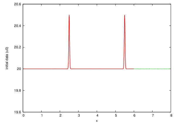
In the next figures we represent the asymptotic stable solutions to system (2.2) on the two-arcs network, produced by our scheme. All the solutions are plotted at a time where the stationary state is already reached. In particular, in Fig. 6 we plot a constant solution obtained using the dissipative transmission coefficients of Section 2.3. In that case we can observe what was explained in Section 2.5, namely that in the case of two arcs and one node, there exist particular dissipative transmission coefficients, such that the asymptotic stationary solutions are constants on all the arcs. In Fig. 7 we plot the more common case of non-constant solutions, obtained using different parameters and non dissipative coefficients. In both cases the limit flux function is equal to zero everywhere, since for the stationary solution the flux is constant, the flux on the external nodes is zero, and all the arcs are connected to external nodes.


Let us now consider a larger network composed of twelve nodes and four arcs, see Fig. 8. We choose some non dissipative transmission coefficients, given in Table 1, in order to satisfy condition (2.8). Let us consider as initial condition on the incoming arc 5, the function plotted in Fig. 9, where we put a small symmetric perturbation of the constant state .
| , | , | , | , | |
| Node S-W | , | , | , | , |
| , | , | , | , | |
| , | , | , | , | |
| , | , | , | , | |
| Node S-E | , | , | , | , |
| , | , | , | , | |
| , | , | , | , | |
| , | , | , | , | |
| Node N-E | , | , | , | , |
| , | , | , | , | |
| , | , | , | , | |
| , | , | , | , | |
| Node N-W | , | , | , | , |
| , | , | , | , | |
| , | , | , | . |

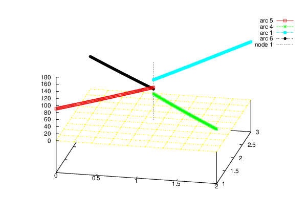
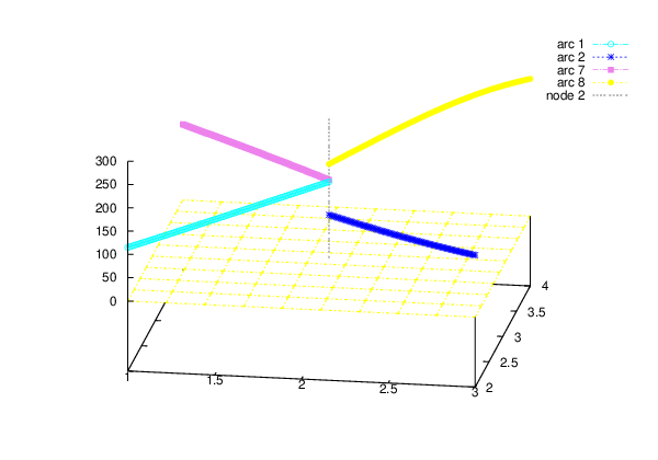
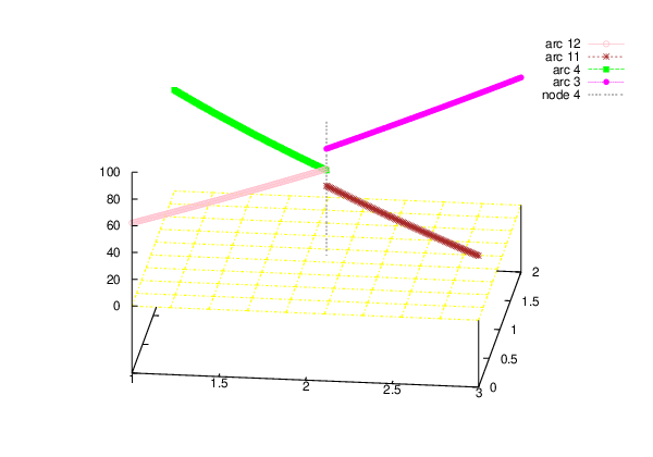
In this case it is hard to compute analytically the stationary solutions. We only know that non-constant solutions are generally expected, according to the discussion in Section 2.5. In Fig. 10 we plot the asymptotic densities on the network node by node, starting from North-East and proceeding in a clockwise direction. Notice that most of the arcs are repeated in the different figures. In Fig. 11 the asymptotic fluxes are represented, and again our scheme is able to stabilize them correctly. We notice that the fluxes of arcs connected to outer boundaries vanish, whereas the fluxes of inner arcs, even if they are constant, are different from zero.
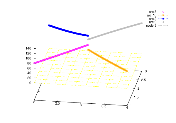

4.3. Instabilities: the appearance of numerical blow-up
Let us consider some cases that present a strong asymptotical instability. Indeed, for some values of the parameters of the problem, namely of the arc’s length and the cell velocity , in connection with the total mass distributed on the arcs of the network, we can observe increasing oscillations, which eventually may cause the blow-up of solutions. It is important to notice that the blow-up can be already observed for this model even for a single arc, see Example 1 below, when the total mass is large with respect to the characteristic parameters and . However, here the presence of more arcs, and so, a greater total length and total mass, makes this kind of phenomenon much more frequent.
Example 1. Here we assume that we have only one interval with and and we take, as initial condition for the density and the chemoattractant, a symmetric perturbation of a constant state . The total mass is , as shown in Figure 12. The solution presents a clear blow-up at time , see Fig. 13. This blow-up seems associated to non physical negative values of the density function , and it is observed in the same way even for refined meshes (see Table 2 for the case of two arcs). This is not surprising, since the quasimonotonicity of the system, see again [24], is violated when the gradient is larger than .


Example 2. Here we take two arcs of length and and the initial density as in Fig. 5, with , , and , . Then we change the values of velocities and in order to see how they influence the behavior of solutions to system (1.1). At the junction we assume transmission and dissipative coefficients, taking and then satisfying equations (2.13)–(2.14). What we observe is that solutions blow up in finite time or not according to the relative values of and , as it is shown in Figure 14. More precisely, we can observe three different regimes. If is large with respect to , solutions stay bounded and converge to stationary solutions (green ”x” in Figure 14). If is small with large enough, then solutions blow up in finite time (red ”+” in Figure 14). Finally, there is a small region in between, around the value 3 and small enough, such that solutions present a large spike at the boundaries (marked by blue asterisks “*”).

Let us now focus on the blow-up behavior. Referring to Fig. 14, we can choose a pair of velocities belonging to the blow-up region marked by red crosses “+“, to say and . The time step just before the numerical blow-up time of corresponding solutions, starting from initial data as in Fig. 5, is plotted in Fig. 15. Even if apparently we are close to the transmission point, there are many grid points separating it from the blow-up point. To show that the blow-up is not just a numerical artifact, we perform the same simulation with the same data, but on refined grids. In Table 2 we report the blow-up time of solutions to system (1.1) for a fixed global mass when either the CFL condition or go to zero. Out of the case of , which appears to be more unstable, the blow-up time is independent of the meshes and has to be considered to occur in the analytical solutions.


| Blow-up time | ||||
4.4. Comparisons and errors
Let us now introduce the formal order of convergence of a numerical method for the computation of the solution as the minimum among the orders on the arcs of the network:
| (4.7) |
where
| (4.8) |
The -error for the numerical solution on each arc is
| (4.9) |
where denotes the numerical solution obtained with the space step discretization equal to , computed in at the final time . The total -error is
| (4.10) |
Table 3 shows the -error (4.9) on the asymptotic solutions , and and order of convergence (4.7) of the approximation scheme applied to the considered network.
| Error on | Error on | Error on | ||||
|---|---|---|---|---|---|---|
| 0.916393 | 1.78849e-04 | 0.965238 | 1.78848e-04 | 1.212334 | 3.34559e-07 | |
| 0.959614 | 8.87206e-05 | 0.982631 | 8.87207e-05 | -0.058657 | 1.44060e-07 | |
| 0.980243 | 4.41941e-05 | 0.990856 | 4.41954e-05 | 0.666605 | 1.49949e-07 | |
| 0.986317 | 2.20550e-05 | 0.992983 | 2.20651e-05 | 0.863690 | 9.43741e-08 | |
| 0.937936 | 1.10172e-05 | 0.937109 | 1.10280e-05 | 0.955806 | 5.17981e-08 |
The results in Table 3 show the effectiveness of AHO approximation scheme in the solution of the transmission problem represented by the hyperbolic model (1.1). We notice indeed that even in this more general case the scheme still keeps a formal accuracy of first order, although the interactions at the boundaries could deteriorate its accuracy.
The research leading to these results has received funding from the European Union Seventh Framework Programme [FP7/2007-2013] under grant agreement n°257462 HYCON2 Network of excellence. This work has also been partially supported by the PRIN project 2008-2009 “Equazioni iperboliche non lineari e fluidodinamica” and by the ANR project MONUMENTALG, ANR-10-JCJC 0103.
References
- [1] D. Aregba-Driollet, M. Briani, and R. Natalini. Asymptotic high-order schemes for dissipative hyperbolic systems, SIAM J. Numer. Anal., 46 (2008), 869–894.
- [2] G. Bretti, R. Natalini and M. Ribot. A numerical scheme for a hyperbolic relaxation model on networks. Numerical Analysis and Applied Mathematics ICNAAM 2011, AIP Conf. Proc. 1389, 1412-1415 (2011);doi: 10.1063/1.3637886.
- [3] A. Chauviere, L. Preziosi. Mathematical framework to model migration of cell population in extracellular matrix, Chapter in ”Cell mechanics. From single scale-based models to multiscale modeling”, A. Chauviere, L. Preziosi and C. Verdier Eds., Taylor & Francis Group, CRC Press publisher, 285-318 (2010)
- [4] R. Dáger and E. Zuazua. Wave propagation, observation and control in flexible multi-structures, volume 50 of Mathématiques & Applications (Berlin) [Mathematics & Applications]. Springer-Verlag, Berlin, 2006.
- [5] Y. Dolak and T. Hillen. Cattaneo models for chemosensitive movement. Numerical solution and pattern formation, J. Math. Biol. 46 (2003), 153–170; corrected version after misprinted p.160 in J. Math. Biol. 46 (2003), 461–478.
- [6] F. Filbet, P. Laurençot, and B. Perthame. Derivation of hyperbolic models for chemosensitive movement. J. Math. Biol., 50(2):189–207, 2005.
- [7] A. Gamba, D. Ambrosi, A. Coniglio, A. de Candia, S. Di Talia, E. Giraudo, G. Serini, L. Preziosi, and F. Bussolino. Percolation, morphogenesis, and Burgers dynamics in blood vessels formation, Phys. Rev. Letters 90 (2003), 118101.1–118101.4.
- [8] M. Garavello and B. Piccoli. Traffic flow on networks, volume 1 of AIMS Series on Applied Mathematics. American Institute of Mathematical Sciences (AIMS), Springfield, MO, 2006. Conservation laws models.
- [9] L. Gosse. Asymptotic-Preserving and Well-Balanced scheme for the 1D Cattaneo model of chemotaxis movement in both hyperbolic and diffusive regimes, preprint, 2010, hal-00528684.
- [10] L. Gosse. Well-balanced numerical approximations display asymptotic decay toward Maxwellian distributions for a model of chemotaxis in a bounded interval, preprint, 2011, hal-00551675.
- [11] J.M. Greenberg and W. Alt. Stability results for a diffusion equation with functional drift approximating a chemotaxis model, Trans. Amer. Math. Soc. 300 (1987), 235–258.
- [12] I. Guaraldo. Some analytical results for hyperbolic chemotaxis model on networks PhD Thesis, Università di Roma “La Sapienza”, 2012.
- [13] F. Guarguaglini and R. Natalini. Nonlinear transmission problems for quasilinear diffusion problems. Networks and heterogeneous media, 2 (2007), 359–381.
- [14] F. Guarguaglini, R. Natalini, C. Mascia and M.Ribot. Stability of constant states and qualitative behavior of solutions to a one dimensional hyper- bolic model of chemotaxis. Discrete Contin. Dyn. Syst. Ser. B, 12 (2009), 39–76.
- [15] T. Hillen. Hyperbolic models for chemosensitive movement. Math. Models Methods Appl. Sci., 12(7): 1007–1034, 2002. Special issue on kinetic theory.
- [16] T. Hillen, C. Rohde, and F. Lutscher, Existence of weak solutions for a hyperbolic model of chemosensitive movement, J. Math. Anal. Appl. 26 (2001), 173–199.
- [17] T. Hillen and A. Stevens. Hyperbolic models for chemotaxis in 1-D. Nonlinear Anal. Real World Appl., 1 (2000), 409–433.
- [18] O. Kedem and A. Katchalsky. Thermodynamic analysis of the permeability of biological membrane to non-electrolytes. Biochimica et Biophysica Acta, 27:229Ð246, 1958.
- [19] E. F. Keller and L.A. Segel. Initiation of slime mold aggregation viewed as an instability. J. Theor. Biol., 26 (1970), 399–415.
- [20] B. A. C. Harley,H. Kim, M. H. Zaman, I. V. Yannas, D. A. Lauffenburger, and L. J. Gibson. Microarchitecture of Three-Dimensional Scaffolds Influences Cell Migration Behavior via Junction Interactions. Biophysical Journal, 29 (2008), 4013–-4024.
- [21] D. Horstmann. From 1970 until present: the Keller-Segel model in chemotaxis and its consequences, I. Jahresber. Deutsch. Math.-Verein. 105 (2003), 103–165.
- [22] B. B. Mandal and S.C. Kundu. Cell proliferation and migration in silk fibroin 3D scaffolds. Biomaterials, 30 (2009) 2956–-2965.
- [23] J. D. Murray. Mathematical biology. I. An introduction. Third edition. Interdisciplinary Applied Mathematics, 17. Springer-Verlag, New York, 2002; II. Spatial models and biomedical applications. Third edition. Interdisciplinary Applied Mathematics, 18. Springer-Verlag, New York, 2003.
- [24] R. Natalini Convergence to equilibrium for the relaxation approximation of conservation laws. Comm. Pure and Appl. Math. 49 (1996), 795–823.
- [25] R. Natalini and M.Ribot. An asymptotic high order mass-preserving scheme for a hyperbolic model of chemotaxis. To appear in SIAM J. Num. Anal.
- [26] B. Perthame. Transport equations in biology, Frontiers in Mathematics, Birkhäuser, 2007.
- [27] L. A. Segel. A theoretical study of receptor mechanisms in bacterial chemotaxis, SIAM J. Appl. Math. 32 (1977), 653–665.
- [28] C. Spadaccio, A. Rainer, S. De Porcellinis, M. Centola, F. De Marco, M. Chello, M. Trombetta, J.A. Genovese. A G-CSF functionalized PLLA scaffold for wound repair: an in vitro preliminary study. Conf Proc IEEE Eng Med Biol Soc., 2010.
- [29] J. Valein and E. Zuazua. Stabilization of the wave equation on 1-D networks. SIAM J. Control Optim., 48(4):2771–2797, 2009.