Correction to Partial Fraction Decomposition Coefficients for Chebyshev Rational Approximation on the Negative Real Axis
Abstract.
Chebyshev rational approximation can be a viable method to compute the exponential of matrices with eigenvalues in the vicinity of the negative real axis, and it was recently applied successfully to solving nuclear fuel burnup equations. Determining the partial fraction decomposition (PFD) coefficients of this approximation can be difficult and they have been provided (for approximation orders 10 and 14) by Gallopoulos and Saad in “Efficient solution of parabolic equations by Krylov approximation methods”, SIAM J. Sci. Stat. Comput., 13(1992). It was recently discovered that the order 14 coefficients contain errors and result in times poorer accuracy than expected by theory. The purpose of this note is to provide the correct PFD coefficients for approximation orders 14 and 16 and to briefly discuss the approximation accuracy resulting from the erroneous coefficients.
Key words and phrases:
best rational approximation, CRAM, partial fraction decomposition, matrix exponential2000 Mathematics Subject Classification
41-04, 65F601. Chebyshev rational approximation
This note concerns the computation of matrix exponential based on the Chebyshev rational approximation method (abbreviated cram in [7]) on the negative real axis. In this approach, the matrix exponential is approximated by a rational matrix function , where the rational function is chosen as the best rational approximation of the exponential function on the negative real axis . Let denote the set of rational functions where and are polynomials of order . The cram approximation of order is defined as the unique rational function satisfying
| (1) |
The asymptotic convergence of this approximation on the negative real axis is remarkably fast with the convergence rate , where is called the Halphen constant [4]. It was recently discovered by Stahl and Schmelzer [11] that this convergence extends to compact subsets on the complex plane and also to Hankel contours in . The application of this approximation to computing the matrix exponential was originally made famous by Cody, Meinardus, and Varga in 1969 in the context of rational approximation of on and it was recently resurfaced by Trefethen, Weideman, and Schmelzer [12]. For self-adjoint and negative semi-definite matrices, the method is guaranteed to yield an error bound in 2-norm that corresponds to the maximum error of the rational approximation on the negative real axis. This has also been the main context for scientific applications [2, 9, 10]. Recently, the method has also been successfully applied to non-self-adjoint matrices with eigenvalues near the negative real axis [7, 6]. These specific matrices arise from a reactor physics application, where the changes in nuclide concentrations due to radioactive decay and neutron-induced reactions are governed by a linear system known as the burnup equations.
2. Partial fraction decomposition form
The main difficulty in using cram for computing the matrix exponential is determining the coefficients of the rational function for a given . In principle, the polynomial coefficients of and can be computed with Remez-type methods but this requires delicate algorithms combined with high-precision arithmetics. Fortunately, these coefficients have been computed to a high accuracy by Carpenter et al. for approximation orders and they are provided in [1]. In practical applications, however, it is usually advantageous to employ cram in the partial fraction decomposition (pfd) form. For simple poles, this composition takes the form
| (2) |
where is the limit of the function at infinity, and are the residues at the poles :
| (3) |
Since the coefficients of are real, its poles form conjugate pairs, so the computational cost can be reduced to half for a real variable
| (4) |
and the matrix exponential solution may be approximated as
| (5) |
for a real matrix .
 |
| (a) |
 |
| (b) |
Although the pfd coefficients can in principle be computed from the polynomial coefficients, the computation of the polynomial roots may be ill-conditioned and requires great care. The pfd coefficients for approximation orders 10 and 14 have been provided in [3], and the given coefficients for have been used in several applications including the matrix exponential computing package expokit [10] and the reactor physics code Serpent [5]. However, in the latter context, it was recently observed that these reported coefficients contain errors and do not correspond to the true best approximation [6]. To illustrate this, Figure 1 shows the error of order 14 approximation on the negative real axis computed using two different sets of coefficients: the partial fraction coefficients from [3], with the corresponding approximation denoted by , and the polynomial coefficients from [1], with the corresponding approximation denoted by . According to theory, a necessary and sufficient condition for the best approximation is that the corresponding error function equioscillates, i.e. there exists a set of points where it attains its maximum absolute value with alternating signs. Notice that the approximation computed with the coefficients from [3] does not exhibit this behavior and in addition results in a times poorer accuracy than expected by theory.
After discovering the erroneous behavior induced by the coefficients from [3], partial fraction coefficients for approximation orders and were computed from the polynomial coefficients provided in [1] and subsequently reported in [6]. The computed pfd coefficients are repeated here in Tables 1 and 2. The computations were performed with Matlab’s Symbolic Toolbox using high precision arithmetics with 200 digits to ensure a sufficient accuracy. In Tables 1 and 2 the coefficients have been rounded off to 20 digits. The coefficients in [1] have been also given with 20 digits’ accuracy, and based on our experience, the approximation order is the highest for which this accuracy is sufficient for computing the pfd coefficients. For lower approximation orders, , the pfd coefficients can be accurately computed with the approximative Carathéodory–Fejér method and a Matlab script is provided for this purpose in [8].
| Coefficient | Real part | Imaginary part |
|---|---|---|
| Coefficient | Real part | Imaginary part |
|---|---|---|
3. Analysis of inaccurate pfd coefficients for
To analyze the effect of inaccurate pfd coefficients denoted by and , let denote the corresponding rational approximation. The error caused by the inaccuracies in the pfd coefficients may be estimated
| (6) |
indicating that the error is the greatest in the vicinity of the poles. It can also be seen from Eq. (6) that the inaccuracy related to the poles has a greater impact near the poles, whereas the error related to the residues should begin to dominate the total error farther away from the poles. By comparing the old and the recomputed pfd coefficients for , it can be seen that the poles all agree to about 6 digits whereas the residues agree to about 5 digits. 11 1 Notice that the pfd coefficients in [3] are given for the rational approximation of on and that they have been multiplied by a factor of two making Eq. (37) in [3] equivalent to Eq. (5). The most dramatic discrepancy occurs for the coefficient for which the significands agree to 5 digits but the exponent value given in [3] is , although the correct value is .
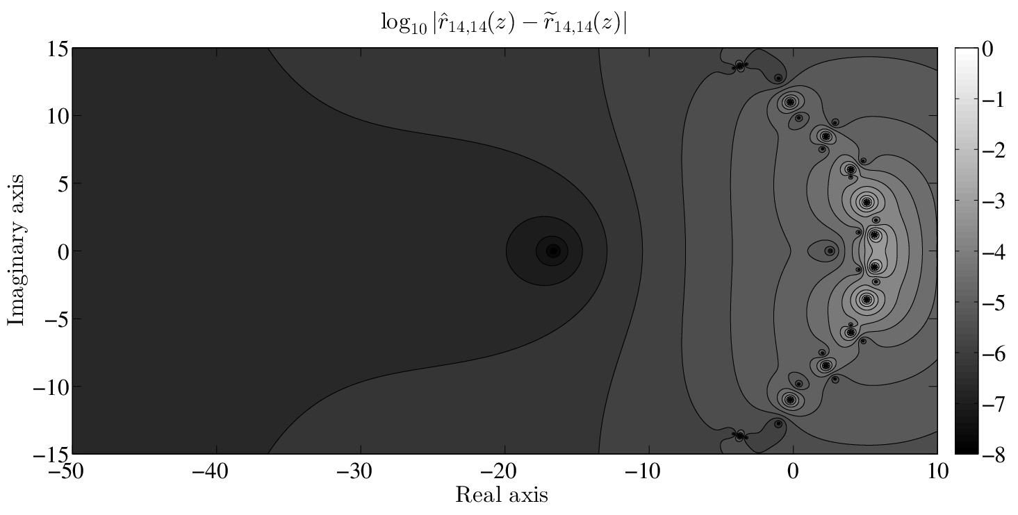
On the grounds of Eq. (6), it can be estimated that coefficients with 6 correct digits should produce a rational function whose deviation from is at most of the order of on the negative real axis. Figure 2 shows the difference between and a rational function that was formed by truncating the pfd coefficients of to 6 significant digits. Interestingly, as can be seen from Fig. 1a, the approximation , corresponding to the pfd coefficients from [3], yields a significantly better accuracy of order than is expected based on the accuracy of the coefficients alone.
To investigate the matter further, let us now take the poles reported in [3] as a starting point for constructing a rational approximation of order 14. The poles define a polynomial
| (7) |
whose values agree to about 6 digits with the values of the correct polynomial on the negative real axis. The residues at the poles cannot be computed in a fully consistent manner, since the poles do not correspond to the true zeros of . However, two alternative approaches for computing the residues can be considered. One possibility is to use the correct rational function and Eq. (3) to compute the residues, but this is inconsistent as Eq. (3) only holds at the true poles. Another option is to define a new rational function using as the denominator and the correct polynomial as the numerator, after which the residues can be computed exactly using symbolic arithmetics. With both of these approaches we obtain a rational approximation, whose accuracy is of the order of on the negative real axis. It is also worth mentioning that forming the rational function based on the poles and the correct residues from Table 1 yields an approximation whose accuracy is of the order of on the negative real axis.
The article [3] by Gallopoulos and Saad does not indicate, how the reported pfd coefficients were computed, but based on the observations regarding the accuracy of the resulting approximation, it is evident that the values given for the residues somehow compensate for the inaccuracies in the poles and it seems likely that they have been optimized to minimize the deviation from on the negative real axis. In fact, using the poles and standard least squares optimization in Matlab with points chosen from the interval , we were able to produce residues yielding only a slightly worse accuracy of order . In any case, it should be noted that optimizing the residues properly in the Chebyshev sense would essentially form a problem of comparable difficulty as the original problem of determining .
References
- [1] A. J. Carpenter, A. Ruttan, and R. S. Varga, Extended numerical computations on the 1/9 conjecture in rational approximation theory, in Rational Approximation and Interpolation, P. R. Graves-Morris, E. B. Saff, and R. S. Varga, eds., vol. 1105 of Lecture Notes in Mathematics, Springer-Verlag, 1984, pp. 383–411.
- [2] W. J. Cody, G. Meinardus, and R. S. Varga, Chebyshev rational approximations to in and applications to heat-conduction problems, J. Approx. Theory, 2 (1969), pp. 50–65.
- [3] E. Gallopoulos and Y. Saad, Efficient solution of parabolic equations by Krylov approximation methods, SIAM J. Sci. Stat. Comput., 13 (1992), pp. 1236–1264.
- [4] A. A. Gonchar and E. A. Rakhmanov, Equilibrium distributions and degree of rational approximation of analytic functions, Math. USSR Sb., 62 (1989).
- [5] J. Leppänen, Serpent, a Continuous-energy Monte Carlo Reactor Physics Burnup Calculation Code, URL: http://montecarlo.vtt.fi, VTT Technical Research Centre of Finland, 2012.
- [6] M. Pusa, Rational approximations to the matrix exponential in burnup calculations, Nucl. Sci. Eng., 169 (2011), pp. 155–167.
- [7] M. Pusa and J. Leppänen, Computing the matrix exponential in burnup calculations, Nucl. Sci. Eng., 164 (2010), pp. 140–150.
- [8] T. Schmelzer, Carathéodory–Fejér approximation, Matlab Central, 2008.
- [9] T. Schmelzer and L. N. Trefethen, Evaluating matrix functions for exponential integrators via Carathéodory–Fejér approximation and contour integrals, Electron. Trans. Numer. Anal., 28 (2007), pp. 1–18.
- [10] R. B. Sidje, Expokit: a software package for computing matrix exponentials, ACM Trans. Math. Softw., 24 (1998), pp. 130–156.
- [11] H. Stahl and T. Schmelzer, An extension of the ‘1/9’-problem, Journal of Computational and Applied Mathematics, 233 (2009), pp. 821–834.
- [12] L. N. Trefethen, J. A. C. Weideman, and T. Schmelzer, Talbot quadratures and rational approximations, BIT., 46 (2006), pp. 653–670.