BA-TH 654-12
Solar System constraints on local dark matter density
Abstract
We study how the classical tests of general relativity are modified by the presence of a subdominant dark matter halo in the solar system. We use a general formalism to calculate the corrected expression for the relevant parameters, and obtain bound plots for the mean energy density and the dimension of the dark matter halo. Our results seem to favor a density profile peaked at the center of the solar system.
pacs
95.35.+d; 98.35.Gi; 04.20.Cv; 95.30.SfI Introduction
It is widely accepted that more than of the matter of our universe is “dark”, a term indicating either that it does not interact with photons, or our lack of knowledge of the profound nature of its constituents. Since the seminal observations by Oort [1] and Zwicky [2] of the early XX century, there have been several independent evidences that some sort of non-baryonic dark matter may exist: the observations of the galactic rotation curves [3] and strong lensing data from Hubble space telescope [4] can be accounted for by the single hypothesis that galaxies are surrounded by a much larger dark matter halo, which contains most of the mass of the galaxies. This is remarkably consistent with the CDM model of our universe, suggested by the WMAP observations [5], which assumes that the mass energy density in our universe is about of the critical energy density, while the observable matter is only , and with various observations on clusters of galaxies, which suggest a “mass-to-light” ratio much higher than . In addition, successful theoretical models and numerical simulations of the formation of structures requires the presence of dark matter.
However, if the existence of dark matter is (almost) commonly accepted, its distribution poses serious challenges. In fact, theoretical models and numerical simulations predict, both for clusters of galaxies [6] and for single galaxies themselves [7, 8] that the radial density profile is quite steep and peaked at the center of the galaxy. But other evidences suggest, on the contrary, that the density profile should be flat, or even shallow [9]. For a comprehensive review of the density profile problem (and many others issue related to dark matter), see [10].
The possibility that the galactic dynamics of massive test particles may be understood without the need for dark matter was also considered in the framework of modified theories of gravity [12, 11, 13]. In particular, the vacuum gravitational field equations in gravity, in the constant velocity region, and the general form of the metric tensor is derived in a closed form was analyzed [12]. The resulting modification of the Einstein-Hilbert Lagrangian is of the form , with the parameter expressed in terms of the tangential velocity. Therefore, it was concluded that in order to explain the motion of test particles around galaxies only requires very mild deviations from classical general relativity, and that modified gravity can explain the galactic dynamics without the need of introducing dark matter. In the context of modified gravity, the virial theorem in gravity was generalized by using the collisionless Boltzmann equation [13]. It was found that supplementary geometric terms in the modified Einstein equation provides an effective contribution to the gravitational energy. Furthermore, the total virial mass was found to be proportional to the effective mass associated with the new geometrical term, which may account for the well-known virial theorem mass discrepancy in clusters of galaxies. The model considered in [13] predicts that the geometric mass and its effects extend beyond the virial radius of the clusters. Thus, it was shown that the virial theorem can be an efficient tool in observationally testing the viability of this class of generalized gravity models.
It is interesting to note that recently the possibility that dark matter is a mixture of two non-interacting perfect fluids, with different four-velocities and thermodynamic parameters was extensively analyzed [14]. By assuming a non-relativistic kinetic model for the dark matter particles, the density profile and the tangential velocity of the dark matter mixture were obtained by numerically integrating the gravitational field equations. The cosmological implications of the model were also briefly considered, and it was shown that the anisotropic two-fluid model isotropizes in the large time limit. In fact, this model was further explored in [15], by assuming that the two dark matter components are pressureless, non-comoving fluids. For this particular choice of the equations of state the dark matter distribution can be described as a single anisotropic fluid, with vanishing tangential pressure, and non-zero radial pressure. The general, radial coordinate dependent, functional relationship between the energy density and the radial pressure was also determined, and it was shown to differ from a simple barotropic equation of state.
Presently, it is considered that the upper bound of the dark matter density in the Solar System is g/cm3 cm-3 [16]. The presence of a local dark matter halo could have some influence on the motion of the objects of the solar system [17, 18, 19]. The problem of the density and distribution of the dark matter in the Solar System is of fundamental importance, not only from a pure theoretical point of view, but also for the design of the dark matter particle detectors. Recently an analysis of the kinematics of 412 stars at 1¡V4 kpc from the Galactic midplane performed in [20] has derived a local density of dark matter that is an order of magnitude below standard expectations, of the order of pc-3, or 0.04 GeV/cm3. This result was contested in [21], where it was claimed that it arises from the invalid assumption that the mean azimuthal velocity of the stellar tracers is independent of the Galactocentric radius at all heights. The assumption of constant mean azimuthal velocity is physically implausible, since it requires the circular velocity to drop more steeply than allowed by any plausible mass model, with or without dark matter, at large heights above the mid-plane [21]. Using the correct approximation that the circular velocity curve is flat in the mid-plane, it was found that the data imply a local dark-matter density of Gev/cm3 [21], consistent with the standard estimates. A new method for the determination of the local disk matter and dark halo matter density was proposed in [22]. The method assumes only that the disc is locally in dynamical equilibrium, and that the ’tilt’ term in the Jeans equations is small up to 1 kpc above the plane. By using this approach a local dark matter density of /pc3 ( GeV/cm3) at 90% confidence level, assuming no correction for the non-flatness of the local rotation curve, and /pc3 ( GeV/cm3), if the correction is included. The obtained lower bound for the local dark matter density is larger than the standard adopted value, and it is inconsistent with the data obtained by extrapolating rotation curves that assume a spherical halo.
In this paper we will consider a different approach to the problem of the dark matter density in the Solar System. If the dark matter density profile follows (roughly) the baryonic matter distribution (for example, because of gravitational interaction), it is plausible to assume that there can be specific features at a much lower scale with respect to the galactic one. In particular, due to some accretion processes, there can be an excess of dark matter around compact objects such as the Sun. Numerical simulation, of course, do not have the resolution to test this hypothesis, but some speculations have been made. A brief review of this particular issue is given in [23]. Our aim is to study how classical tests of general relativity, i.e., the precession of the perihelion of the planet Mercury, the deflection of light rays and the delay of radio signals passing close to the Sun, are modified by the presence of a local, subdominant dark matter energy density distribution. The Solar System tests are very powerful tools for testing different gravitational models, as well as the theoretical extensions of General Relativity, and they have been applied recently to a variety of contexts [24, 25, 26].
The present paper is organized as follows. In Section II, we derive an approximate expression for the space-time metric of the Solar System in the presence of dark matter. In Section III we use this expression, and the formalism of Section A to evaluate the corrections due to the presence of dark matter to the relevant parameters in the Solar System gravitational tests. Finally in Section IV, we discuss our results and draw our conclusions. In the Appendix we describe the general formalism used to evaluate the observational parameters of physical interest.
II Metric of a static dark matter halo surrounding the Sun
Throughout this work, we assume a general metric of the form
| (1) |
which will be used to obtain the general expressions for the classical tests of general relativity, namely, for the precession of the perihelion of Mercury, for the deflection of light rays passing close to the Sun and for the radar echo delay observations. For the Schwarzschild metric, giving the spherically symmetric vacuum solution of the Einstein gravitational field equations, the functions and are given by
| (2) |
where is the Schwarzschild radius, with the mass of the central object.
We begin this Section by deriving an approximate expression for the metric of a space-time filled by static dark matter around a star, by using an ansatz of the form (1). We assume that the dark matter source is described by a perfect fluid stress-energy tensor
| (3) |
where and are related by the equation of state , constant (later on, we will set according to the general equation of state of the matter source). The Einstein field equations reduce to two independent differential equations (we set
| (4) | |||||
| (5) |
We assume that energy density and pressure of dark matter are very small, and , and hence the presence of dark matter can be regarded as a small perturbation of the vacuum state. Therefore we can expand the metric around the Schwarzschild solution as
| (6) | |||||
| (7) |
with and given by Eq. (2). Then, after some algebraic manipulation, using the leading order equation of motion and neglecting higher order terms, Eq.(4) becomes
| (8) |
By defining the effective mass function (see, for example, [27])
| (9) |
from Eq. (8) we obtain the function as
| (10) |
where we have expressed the gravitational coupling constant in terms of the mass and of the Schwarzschild radius. By using the definition of the effective mass and the equation of state of the matter, we can relate and with the derivative of . Then, after some algebra and using again leading order equations of motion and solutions, Eq. (5) becomes
| (11) |
where the prime denotes a derivative with respect to .
Now, using the conservation equation to get another independent equation relating the metric and the effective mass would be an unnecessary effort, since the barotropic assumption is too constrictive to get a realistic energy distribution, and the resulting equations of motion are too difficult to handle. We will instead use, for the dark matter energy density, an effective distribution, inspired by the Navarro-Frenk-White profile for the energy density of the galactic halos [19]
| (12) |
where and are constant arbitrary parameters related to the mean density and the dimension of the star halo, and is assumed to be a constant. We set , as usual for pressureless matter sources. Then the effective mass function and the metric function can be easily evaluated, and are provided by the following relationships
| (13) | |||||
| (14) |
A closed expression for can not be found. However, the general solution of Eq. (11) is given by
| (15) |
Though it is reasonable to assume , there is no need in principle to set another limit to , since our approximation holds only outside the Sun, and a matter distribution like (12) can be trusted up to a cutoff radius (for example the virial radius in the NFW distribution). Nevertheless, the analysis we are proposing makes sense only if the contribution to the metric around the Sun from dark matter is actually localized in the Solar System. Thus, we do expect the corrections to the metric functions to vanish as , and so we will assume for simplicity .
In the next Section, we will use the approximated metric we have deduced to see how the classical tests of general relativity constrain the form of the dark matter distribution.
III Classical tests of General Relativity in the Dark Matter halo
In Appendix A, we briefly review the formalism used in studying the classical tests of general relativity, which we have included for self-consistency and self-completeness. The formalism is completely general, and can be used to treat any static spherically symmetric metric [25, 26].
In this Section, we will use the metric given by Eqs. (14) - (15) to study how the results of the classical tests of General Relativity (perihelion precession, light deflection and radar echo delay) are modified in the Solar System due to the presence of the dark matter. Let us first write down the metric functions in terms of the variable ,
| (16) |
and
| (17) |
respectively.
III.1 Perihelion precession
In order to obtain the change in the perihelion precession due to the presence of dark matter we need to evaluate the function , where is the standard GR result, given in (51), and is the first order perturbation generated from the modification of the metric functions, which can be written as
| (18) |
Plugging into this equation the expressions of the metric functions (16)-(17), we arrive at
| (19) | |||||
and
| (20) | |||||
respectively. In the small velocity limit, , so that (higher order would be subleading in our expansion), and we can write
| (21) |
Using for and the values given in Eqs. (50)-(60) respectively, the perihelion precession angle can be written as
| (22) | |||||
The observed value of the perihelion precession for the planet mercury is arcsec per century [28], while the predicted value from GR is arcsec per century. Assuming that the entire discrepancy is due to the presence of dark matter, we obtain the following constraint for the mean density and the radius of the dark matter subhalo
| (23) |
where and are, respectively, the periods of revolution of Mercury and of the Earth.
III.2 Light deflection
To obtain the correction to the deflection of light given by the presence of dark matter around the Sun, we must solve the general equation (58). By defining , where is the straight line solution and is the GR result (65), we can write the equation as
| (24) |
with the functions and obtained from the first order corrections to the metric functions due to dark matter11 1 In the right hand side of Eq. (24) we have dropped the term , since it is of order , and can thus be neglected. For the function we obtain
| (25) |
so that, by inserting the solutions (16)-(17), the functions and are given by
| (26) | |||||
| (27) | |||||
respectively.
Keeping only the leading order in the expansion, we can again set and . Then, inserting the expression of in (27), we can write Eq. (24) as
| (28) |
The solution of this equation is
| (29) |
The condition now yields
| (30) |
where
| (31) |
is the Euler’s function [35].
Since we have assumed , we can discard the term in the previous equation, so that we are left with a simple linear equation. Finally, the deflection angle can be evaluated as
| (32) |
The best available data on light deflection by the Sun come from long baseline radio interferometry [29], which gives , with arcsec. Thus, assuming, as usual, that all the discrepancy is due to the dark matter correction, and taking , we obtain the following constraint
| (33) |
III.3 Radar echo delay
To obtain the expression of the radar echo delay in the presence of the dark matter sub halo, we have to evaluate the integral (67) with the corrected metric functions. Since we can set
| (34) |
by neglecting higher order terms we obtain
| (35) |
Therefore the correction to the standard GR result can be set as
| (36) | |||||
where is the Hypergeometric function [35], defined as the solution of the differential equation
| (37) |
Observational constraints on the radar echo delay comes form the frequency shift of radio photons to and from the Cassini spacecraft [30]. We have , with . Therefore, assuming as usual that the discrepancy is completely due to the presence of dark matter, we obtain the constraint
| (38) |
The next Section will be devoted to some comments on the above results, and we will draw our conclusions.


IV Comments and conclusions
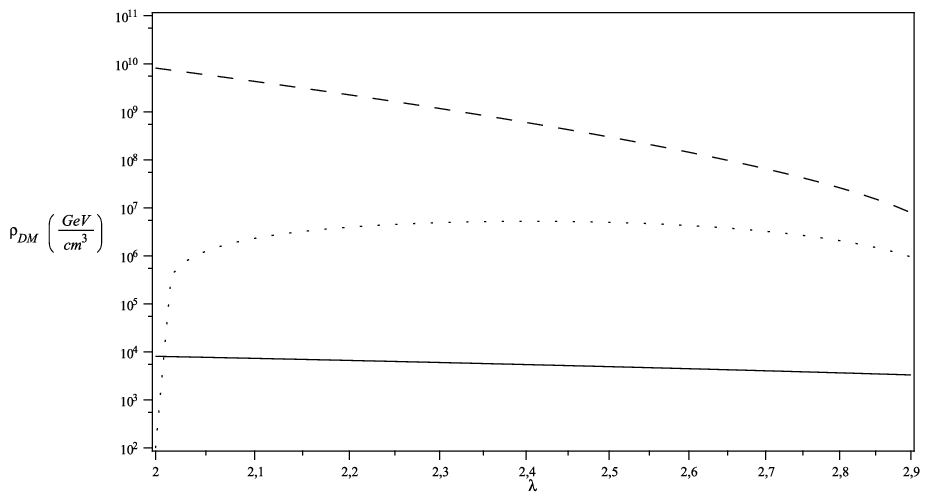
In the previous Section we have evaluated the possible influence that the presence of Sun-bound dark matter could have on the classical tests of general relativity. The results we obtained are summarized in Figs. 1 and 2.
As we can see, the most constraining test is always the study of the perihelion precession. The results strongly depends on the extension of the dark matter halo (Fig. 1). If the distribution is extremely concentrated around the Sun, the effect become more and more negligible. On the contrary, for halos extending roughly to the orbit of the Earth, the constraint on the mean dark density becomes comparable with the results obtained by other authors [17, 18, 19]. For halos as big as the planetary solar system, the constraint on the mean dark matter energy becomes tighter. On the contrary, at least for what concerns the perihelion precession, the -dependence is quite mild (Fig. 2). Notice that for very large values of the bounds obtained becomes comparable with what is expected from the mean energy density distribution of the galaxy [31]. This is a consequence of the choice of our hypothesis for the energy density distribution (12), which do not constraint the total amount of dark matter around the Sun. Nevertheless, we can argue that, if some sort of overdensity can be localized around the Sun, a distribution packed close to the Sun seems to be less in tension with observations.
Some considerations on how the analysis we have performed can be improved seems appropriate. Of course, assuming that the dark matter distribution is static is certainly not true. Probably a model of rotating dark matter could improve the constraints, but the metric would be quite complicated. In fact, no exact non-empty spherically symmetric rotating solution is known. As a future work, it could be possible to perform a similar analysis, using the Kerr geometry as the background expansion. For what concerns the profile energy density, we believe that the expression we have used could capture the essential features of a more realistic energy density distribution, especially because we are mainly interested in the dimension and the mean density of such a distribution. From this point of view, we think that our results are robust. A different but still interesting issue would be to take into account the possibility of dark matter “streams” of extragalactic objects recently captured by our galaxy, which could give some strong local overdensities, and which could be characterized by a definite velocity pattern. Maybe it could be possible to model such an effect, for example via an Einstein cluster approach [32]. This will also be the object of future investigations.
In conclusion, our analysis suggest that indirect gravitational effect originated by dark matter can be interesting even at small scales, and can be a useful cross-check for direct detection experiments.
Acknowledgments
We would like to thank Pasquale Dario Serpico for useful discussion, and Maurizio Gasperini for helpful comments on the manuscript. The work of TH was supported by an GRF grant of the government of the Hong Kong SAR. FSNL acknowledges financial support of the Fundação para a Ciência e Tecnologia through the grants CERN/FP/123615/2011 and CERN/FP/123618/2011.
Appendix A Classical tests of General Relativity in an arbitrary spherically symmetric static space-time
In this Appendix, we briefly review the formalism used in studying the classical tests of general relativity. This formalism is completely general, and can be used to treat any static spherically symmetric metric [25, 26]. The Appendix follows closely the line of the analogous Section of [26], and we include it for self-completeness and self-consistency. The general metric of the form
| (39) |
which will be used to obtain a general expressions for the classical tests of general relativity. For the Schwarzschild metric the functions and are given by Eqs. (2).
A.1 Perihelion precession
The motion of a test particle in the gravitational field described by the metric given by Eq. (39) can be derived from the variational principle
| (40) |
where the dot denotes . It is easy to see that the orbit must be planar, and hence we can set without any loss of generality. Therefore we will use as the angular coordinate. Since neither nor appear explicitly in Eq. (40), their conjugate momenta yield constants of motion (related respectively with energy and angular momentum conservation)
| (41) |
From (40), using the constants of motion (41), changing the variable and expressing the affine derivative as an angular derivative we arrive at the equation
| (42) |
By taking the derivative of the previous equation with respect to we find
| (43) |
where
| (44) |
A circular orbit is given by the root of the equation . Any deviation from a circular orbit must satisfy the equation
| (45) |
which is obtained by substituting in Eq. (43). Therefore, to first order in , the trajectory is given by
| (46) |
where and are constants of integration. The angles of the perihelia of the orbit are the angles for which is minimum and hence or is maximum. Therefore, the variation of the orbital angle from one perihelion to the next is
| (47) |
The parameter defined by the above equation represents the perihelion advance, giving the rate of the perihelion change. As the planet advances through radians in its orbit, its perihelion advances through radians. From Eq. (47), is given by
| (48) |
or, for small , by
| (49) |
For a complete rotation we have , and the advance of the perihelion is . In order to be able to perform effective calculations of the perihelion precession we need to know the expression of as a function of the orbit parameters. If the planet is moving on a Keplerian ellipse with semi-axis , and eccentricity of the orbit is , then [25, 26]
| (50) |
As an example of the application of the present formalism, and for future references, we consider the precession of the perihelion of a planet in the Schwarzschild geometry, where we have
| (51) | |||||
| (52) |
The radius of the circular orbit is obtained as the solution of the quadratic algebraic equation
| (53) |
with the only physical solution given by
| (54) |
A.2 Deflection of light
In the absence of external forces a photon follows a null geodesic, . The affine parameter along the photon’s path can be taken as an arbitrary quantity, and we denote again by a dot the derivatives with respect to the arbitrary affine parameter. There are two constants of motion, the energy and the angular momentum , given again by eqs. (41).
The equation of motion of the photon is
| (56) |
which, with the use of the constants of motion, the change of variable and the use of the conservation equations to eliminate the derivative with respect to the affine parameter leads to
| (57) |
By taking the derivative of the previous equation with respect to we find
| (58) |
where
| (59) |
In the lowest approximation, in which the term of the right hand side of the equation (58) is neglected, the solution is a straight line,
| (60) |
where is the distance of the closest approach to the mass. In the next approximation Eq. (60) is used on the right-hand side of Eq. (58), to give a second order linear inhomogeneous equation of the form
| (61) |
with a general solution given by . The light ray comes in from infinity at the asymptotic angle and goes out to infinity at an asymptotic angle . The angle is obtained as a solution of the equation , and the total deflection angle of the light ray is .
A.3 Radar echo delay
The time travel of a light signal changes in the presence of a gravitational field. The time difference can be cast as
| (67) |
where we can set , with being the distance of closest approach.
In the case of the Schwarzschild metric we have
| (68) |
By assuming that the sources are far enough, and , and we have [34]
| (69) |
References
- [1] J.H. Oort, Bulletin of the Astronomical Institutes of the Netherlands 6, 249 (1932).
- [2] F. Zwicky, Astrophys. J. 86, 246 (1937).
- [3] V. C. Rubin and W. K. Ford, Jr., Astrophys. J. 159, 379 (1970); K. G. Begeman, A. H. Broeils and R. H. Sanders, Mon. Not. Roy. Astron. Soc. 249, 523 (1991).
- [4] M. J. Hudson, S. D. J. Gwyn, H. Dahle and N. Kaiser, Astrophys. J. 503, 531 (1998) [astro-ph/9711341].
- [5] E. Komatsu et al. [WMAP Collaboration], Astrophys. J. Suppl. 192, 18 (2011) [arXiv:1001.4538 [astro-ph.CO]].
- [6] J. F. Navarro, C. S. Frenk and S. D. M. White, Astrophys. J. 490, 493 (1997) [astro-ph/9611107].
- [7] P. Salucci and A. Borriello, Lect. Notes Phys. 616, 66 (2003) [astro-ph/0203457].
- [8] D. Reed, F. Governato, L. Verde, J. Gardner, T. R. Quinn, J. Stadel, D. Merritt and G. Lake, Mon. Not. Roy. Astron. Soc. 357, 82 (2005) [astro-ph/0312544].
- [9] W. J. G. de Blok, S. S. McGaugh, A. Bosma and V. C. Rubin, Astrophys. J. 552, L23 (2001) [astro-ph/0103102].
- [10] G. Bertone, D. Hooper and J. Silk, Phys. Rept. 405, 279 (2005) [hep-ph/0404175].
- [11] S. Capozziello, V. F. Cardone and A. Troisi, JCAP 0608, 001 (2006); S. Capozziello, V. F. Cardone and A. Troisi, Month. Not. R. Astron. Soc. 375, 1423 (2007); A. Borowiec, W. Godlowski and M. Szydlowski, Int. J. Geom. Meth. Mod. Phys. 4, 183 (2007). [28] C. F. Martins and P. Salucci, Mon. Not. Roy. Astron. Soc. 381, 1103 (2007).
- [12] C. G. Boehmer, T. Harko and F. S. N. Lobo, Astropart. Phys. 29, 386 (2008) [arXiv:0709.0046 [gr-qc]].
- [13] C. G. Boehmer, T. Harko and F. S. N. Lobo, JCAP 0803, 024 (2008) [arXiv:0710.0966 [gr-qc]].
- [14] T. Harko and F. S. N. Lobo, Phys. Rev. D 83, 124051 (2011) [arXiv:1106.2642 [gr-qc]].
- [15] T. Harko and F. S. N. Lobo, Astropart. Phys. 35, 547 (2012) [arXiv:1104.2674 [gr-qc]].
- [16] L. Iorio, Journal of Cosmology and Astroparticle Physics 05, 018 (2010).
- [17] M. Sereno and P. .Jetzer, Mon. Not. Roy. Astron. Soc. 371, 626 (2006) [astro-ph/0606197].
- [18] L. Iorio, JCAP 0605, 002 (2006) [gr-qc/0602095].
- [19] J. -M. Frere, F. -S. Ling and G. Vertongen, Phys. Rev. D 77, 083005 (2008) [astro-ph/0701542].
- [20] C. Moni Bidin, G. Carraro, R. A. Mendez, and R. Smith, Astrophys. J. 751, 30 (2012).
- [21] J. Bovy and S. Tremaine, arXiv:1205.4033v1 (2012).
- [22] S. Garbari, C. Liu, J. I. Read,and G. Lake, arXiv:1206.0015 (2012).
- [23] S. L. Adler, arXiv:0903.4879 [astro-ph.EP].
- [24] C. G. Boehmer, T. Harko and F. S. N. Lobo, Class. Quant. Grav. 25, 045015 (2008) [arXiv:0801.1375 [gr-qc]].
- [25] T. Harko, Z. Kovacs and F. S. N. Lobo, Proc. Roy. Soc. Lond. A Math. Phys. Eng. Sci. 467, 1390 (2011) [arXiv:0908.2874 [gr-qc]].
- [26] C. G. Boehmer, G. De Risi, T. Harko and F. S. N. Lobo, Class. Quant. Grav. 27, 185013 (2010) [arXiv:0910.3800 [gr-qc]].
- [27] M. P. Hobson, G. P. Efstathiou and A. N. Lasenby, General relativity: An introduction for physicists, Cambridge University Press, United Kingdom, p. 572 (2006).
- [28] I. I. Shapiro, W. B. Smith, M. E. Ash and S. Herrick, Astron. J. 76, 588 (1971); I. I. Shapiro, C. C. Counselman and R. W. King, Phys. Rev. Lett. 36, 555 (1976).
- [29] D. S. Robertson, W. E. Carter and W. H. Dillinger, Nature 349, 768 (1991); D. E. Lebach, B. E. Corey, I. I. Shapiro, M. I. Ratner, J. C. Webber, A. E. E. Rogers, J. L. Davis, and T. A. Herring, Phys. Rev. Lett. 75, 1439 (1995).
- [30] R. D. Reasenberg, I. I. Shapiro, P. E. MacNeil, R. B. Goldstein, J. C. Breidenthal, J. P. Brenkle, D. L. Cain, T. M Kaufman, T. A. Komarek and A. I. Zygielbaum, Astrophys. J. 234L, 219 (1979); B. Bertotti, L. Iess, and P. Tortora, Nature 425, 374 (2003).
- [31] R. Catena and P. Ullio, JCAP 1008, 004 (2010) [arXiv:0907.0018 [astro-ph.CO]].
- [32] C. G. Boehmer and T. Harko, Mon. Not. Roy. Astron. Soc. 379, 393 (2007).
- [33] L. D. Landau and E. M. Lifshitz, The classical theory of fields, Oxford, Pergamon Press (1975).
- [34] I. I. Shapiro, W. B. Smith, M. E. Ash and S. Herrick, Astron. J. 76, 588 (1971); I. I. Shapiro, C. C. Counselman and R. W. King, Phys. Rev. Lett. 36, 555 (1976).
- [35] I. S. Gradshteyn, I. M. Ryzhik, “Table of Integrals, Series, and Products” Alan Jeffrey and Daniel Zwillinger (eds.) Seventh edition (Feb 2007) 1171 pages