Semiparametric Mixed Model for Evaluating Pathway-Environment Interaction

Let us consider that we have a total of $n$ subjects and the $i$th subject has a continuous disease-related outcome $y_{i},i=1,2,...n$. We are interested in relating this response $\mathbf{y}=(y_{1},y_{2},...,y_{n})^{T}$ with one particular pathway gene expression data $Z=({\boldsymbol{z}}_{1},{\boldsymbol{z}}_{2},...,{\boldsymbol{z}}_{n})^{T}$ and $k$ environmental variables. In a general form, we can write this nonlinear relationship as

where $\boldsymbol{\epsilon}$ and $\mathbf{f}$ are $n\times 1$ dimensional vectors with a specific relationship with $\mathbf{y}$ for the $i$th entry as $y_{i}=f({\boldsymbol{x}}^{T}_{i},{\boldsymbol{z}}^{T}_{i})+\epsilon_{i}$, in which ${\boldsymbol{x}}^{T}_{i}=(x_{i1},x_{i2},...,x_{ik})$ is $1\times k$ vector of environmental variables and ${\boldsymbol{z}}^{T}_{i}=(z_{i1},z_{i2},...,z_{ip})$ is the $1\times p$ vector of gene expression within a pathway and $p$ is the gene number. In this paper, we only consider the case with one environmental variable, i.e., $k=1$ so that the input $\boldsymbol{x}^{T}$ is reduced to univariate $x$. We assume that the errors $\boldsymbol{\epsilon}\sim N(0,\sigma^{2}I)$ are $n\times 1$ iid random variables vector. $f(\cdot)$ denotes the unknown non-linear smooth functions for $x_{i}$, ${\boldsymbol{z}}^{T}_{i}$, and their interaction. In this paper, we assume function $f$ has the following form:

where $\beta_{0}$ is the intercept term, and $f_{\alpha},\alpha\in\{x,z,xz\}$, represents the nonlinear effect of the environmental variable, the pathway or the interaction respectively. The above equation is similar to the additive model with two univariate variables and their interaction, except ${\boldsymbol{z}}^{T}$ is a multivariate variable. By writing the general model (1) in this way, we can estimate $f_{x}$, $f_{z}$ and their interaction $f_{xz}$ separately according to the characteristics of the pathway and the environmental variable. We model $f_{x}(x)$ using the nonparametric function such as a cubic smoothing spline (Wahba, 1990; Lin and Zhang, 1999; Zhang and Lin, 2003). To handle the high dimensional pathway covariates, ${\boldsymbol{z}}^{T}$, we may consider a Gaussian process to express $f_{z}({\boldsymbol{z}}^{T})$ since the least squares kernel machine method with the Gaussian kernel has achieved success in a genetic pathway data analysis (Liu et al., 2007).

Before we derive the specific representation for the interaction function, we need examine the function space of $f_{x}$ and $f_{z}$ respectively. For the smoothing spline $x\in\mathcal{T}=[0,1]$, $f_{x}$ is spanned on the function space $\mathcal{H}_{x}=\mathcal{H}_{x}^{0}\bigoplus\mathcal{H}_{x}^{1}$, where “$\bigoplus$”, $\mathcal{H}_{x}^{0}$ and $\mathcal{H}_{x}^{1}$ represent the direct sum operator of two subspaces, the null function space and the penalized function space respectively (Wahba, 1990). Assuming $n$ distinct values of $x_{i}$ such that $0<x^{0}_{1}<\cdots<x^{0}_{n}<1$, the $m$th order smoothing spline estimator $f_{x}(x)$ can be expressed as (Wahba, 1990; Zhang and Lin, 2003),

where $\phi_{j}(x)$ is the polynomial basis that span the null space $\mathcal{H}_{x}^{0}$ with $\phi_{j}(x)=x^{j-1}/(j-1)!,j=1,2,\dots,m$, and $k_{x}(x,x^{0}_{i})=[(m-1)!]^{-2}\int(x-u)^{m-1}_{+}(x^{0}_{i}-u)_{+}^{m-1}du$ is the kernel which uniquely determines the space $\mathcal{H}_{x}^{1}$. For $m=2$, the natural cubic spline that we shall apply in our model, the kernel of $\mathcal{H}_{x}^{1}$ can be calculated as (Hastie et al., 2009; Rasmussen and Williams, 2006)

where subscript “+” indicates the positive part of the expression. For the null space $\mathcal{H}_{x}^{0}$, the kernel is calculated as $k^{0}_{x}(x,x^{\prime})=\sum_{j=1}^{2}\phi_{j}(x)\phi_{j}(x^{\prime})=1+xx^{\prime}$.

With the orthonormal polynomial basis, $\mathcal{H}_{x}^{0}=\{1\}\bigoplus\{x\}$, where $\{1\}$ and $\{x\}$ stand for the linear function spaces spanned by the constant 1 and the linear basis $x$ which is centered (Guo, 2002). Since the kernel of the function space of the direct sum of two subspaces is expressed by the direct sum of the kernel of the subspaces (Aronszajn, 1950; Wahba, 1990), we can derive the kernel of the function space without the the constant term for the cubic smoothing spline, $\{x\}\bigoplus\mathcal{H}_{x}^{1}$, as $[xx^{\prime}+k_{x}(x,x^{\prime})]$.

For the function space of $f_{z}$, we consider a similar argument by MacKay (1998) that starting from a parametric model, we can span the function of $f_{z}$ by a radial basis

where $\phi_{h}({\boldsymbol{z}}^{T})=\exp\left[-{\|{\boldsymbol{z}}-{\boldsymbol{z}}_{h}\|^{2}}\over{2\rho}\right]$ is the radial basis functions centered at fixed points $\{{\boldsymbol{z}}_{h}\}_{h=1}^{H}$. Assuming $\mathbf{c}=(c_{1},...,c_{h})^{T}\sim N(0,\tau_{z}I)$, the entry of the covariance matrix of $\mathbf{f}_{z}$ is expressed as

Taking as an example a one-dimensional case, MacKay (1998) shows that in the above expression the sum over $h$ becomes an integral when taking the limit $H\rightarrow\infty$ such that $R=\tau_{z}\exp\left[-(z-z^{\prime})^{2}/\rho\right]$. Generalizing from this particular case, we can define the Gaussian kernel of the function space $\mathcal{H}_{z}^{1}$ on ${\boldsymbol{z}}$

and we assume that $f_{z}$ is generated from a zero mean Gaussian process with the kernel matrix produced by $k_{z}$.

Since the tensor product of the kernels of two function spaces determines a new function space (Aronszajn, 1950), we use the tensor product of the kernels of $\{x\}\bigoplus\mathcal{H}_{x}^{1}$ and $\mathcal{H}_{z}^{1}$ to construct a new function space, $\mathcal{H}_{xz}^{1}$, which contains any order interaction $f_{xz}$ between $x$ and ${\boldsymbol{z}}^{T}$. Now we can express the kernel of the interaction function space as

Therefore, we are able to represent the nonparametric interaction function using a zero mean Gaussian process with the kernel matrix produced by this kernel function.

In the rest of this paper, we use $K_{x}$, $K_{z}$ and $K_{xz}$ to stand for the Gram or kernel matrices produced by $k_{x},k_{z}$ and $k_{xz}$ respectively. In a specific problem, the environmental variable $x$ must be scaled into $\mathcal{T}=[0,1]$ to construct the interaction kernel. Notice the model expression (2) is not the analysis of variance (ANOVA) decomposition of the smoothing function $f$ since $\mathcal{H}_{z}^{1}$ and $\mathcal{H}_{xz}^{1}$ are not orthogonal to each other. This may cause the identifiability problem between $f_{z}$ and $f_{xz}$. However, in practice, this problem only happens to our model in extreme situations such as when the entries of matrix $xx^{\prime}+k_{x}(x,x^{\prime})$ are close to each other. In general, $f_{z}$ and $f_{xz}$ can be identified well as shown in the simulation and application study.

Now we are prepared to pose the optimization problem. Based on the above argument, the corresponding function spaces that are penalized are $\mathcal{H}_{x}^{1}$, $\mathcal{H}_{z}^{1}$ and $\mathcal{H}_{xz}^{1}$. Analogous to the additive models (Hastie and Tibshirani, 1990), the estimation problem for model (1) becomes: for a given set of predictors $(x_{i},\boldsymbol{z}_{i}^{T}),i=1,2,...,n$, find $f$ to maximize

where $\|f_{\alpha}\|_{\mathcal{H}^{1}_{\alpha}}$’s are the norms induced by $K_{\alpha}$ of $\mathcal{H}_{\alpha}^{1},\alpha\in\{x,z,xz\}$, and $\lambda_{\alpha}$’s are the penalty parameters that balance the tradeoff between goodness-of-fit and smoothing of the curve or high dimensional surface. The solutions to expression (7) are called the least square kernel machine estimation, and Liu et al. (2007) showed the equivalence of the least square kernel machine to the linear mixed model without interaction effects.

The model (2) can be represented in terms of a mixed model as follows. According to the Representer Theorem (Kimeldorf and Wahba, 1971), the nonparametric function can be expressed by the kernel, $f_{z}(\cdot)=\sum_{i=1}^{n}a_{i}k_{z}(\cdot,\boldsymbol{z}^{T}_{i})$ and $f_{xz}(\cdot)=\sum_{i=1}^{n}b_{i}k_{xz}(\cdot;x_{i},{\boldsymbol{z}}^{T}_{i})$. So the vectors of these functions are

where $a_{i}\in\mathbb{R},b_{i}\in\mathbb{R}$. Based on the properties of reproducing kernels, the squared norms of $\mathcal{H}_{z}^{1}$ and $\mathcal{H}_{xz}^{1}$ can be expressed as

To represent the remaining part of model (2), $\beta_{0}+f_{x}(\cdot)$, we follow Lin and Zhang (1999); Zhang et al. (1998); Green (1987); Green and Silverman (1994)’s procedure. The vector of $f_{x}$, $\mathbf{f}_{x}$ (note here the constant $\beta_{0}$ is absorbed into $f_{x}$), can be expressed in terms of $\boldsymbol{\beta}=(\beta_{0},\beta_{1})^{T}$ and $(n-2)\times 1$ random vector $\mathbf{r}_{x}$ as

for $n$ distinct input $x$ values, where $\mathbf{r}_{x}\sim N(0,\tau_{x}I)$ and $X$ is the design matrix of the null space $\mathcal{H}_{x}^{0}$ spanned by the orthogonal polynomial basis, i.e., $X=(\mathbf{1},\mathbf{x})$ and $\mathbf{x}$ is the $n\times 1$ vector of centered $x$. $B$ is a matrix defined as $B=L(L^{T}L)^{-1}$, where $L$ is $n\times(n-2)$ full rank matrix with $M=LL^{T}$. $M$ is a penalty matrix defined by Green and Silverman (1994) such that the squared norm of $\mathcal{H}_{x}^{1}$,

More details to define $B$ and $M$ can be found in Green and Silverman (1994), Zhang et al. (1998) and Appendix A.

Plugging those representations of square norms and $\mathbf{f}_{\alpha}$’s back into (7), we have

If we define $\lambda_{x}=\sigma^{2}/\tau_{x},\lambda_{z}=\sigma^{2}/\tau_{z}$ and $\lambda_{xz}=\sigma^{2}/\tau_{xz}$, and have random vectors $\mathbf{r}_{z}=\mathbf{f}_{z},\mathbf{r}_{z}\sim N(0,\tau_{z}K_{z})$ and $\mathbf{r}_{xz}=\mathbf{f}_{xz},\mathbf{r}_{xz}\sim N(0,\tau_{xz}K_{xz})$, then the above equation is equivalent to

which is the triple penalized log likelihood function of the linear mixed model

From the Bayesian point-of-view, $\mathbf{f}$ is interpreted as the sum of four zero-mean stationary Gaussian processes, each with a prior covariance function $\tau_{\alpha}K_{\alpha}$ ($\boldsymbol{\beta}$ can be viewed with infinite variance). The vectors $\mathbf{r}_{z}$ and $\mathbf{r}_{xz}$ have more specific meanings as the pathway main effect and the P-E interaction effect. Although $\mathbf{r}_{x}$ does not have such a meaning, it can be interpreted as the nonlinear contribution of the relationship of the response and the environmental variable.

Differentiating expression (12) with respect to $\boldsymbol{\beta}$ and $\mathbf{r}_{\alpha}$’s, it is easy to show that the best linear unbiased prediction (BLUP) estimate of the random effects, given $\sigma^{2}$ and $\tau_{\alpha}$’s as fixed, is obtained from solving

Equation (13) shows that the BLUP estimate of $\boldsymbol{\beta}$ and $\mathbf{r}_{\alpha}$’s are unique if $X^{T}X$ is full rank which is usually satisfied.

Given the fixed parameters $\sigma^{2}$ and $\tau_{\alpha}$’s, the covariance of $\mathbf{y}$ is obtained as follows using model (12),

Instead of solving expression (13) directly, we perform recursive steps to simultaneously achieve the approximate expressions of $\boldsymbol{\beta}$ and $\mathbf{r}_{\alpha}$’s, $\alpha\in\{x,z,xz\}$,

where $I$ is the $(n-2)\times(n-2)$ identity matrix, and $\Delta_{j},\;j=1,2,3$, are covariances for the following distributions,

The above expressions for $\hat{\boldsymbol{\beta}}$ and $\hat{\mathbf{r}}_{\alpha}$’s are all linear transformations of $\mathbf{y}$; thus, their covariances are easily determined using identity $\hbox{Cov}(A\mathbf{y})=A\hbox{Cov}(\mathbf{y})A^{T}=A\Sigma A^{T}$, where $A$ is the transformation matrix in expressions (15).

In the previous Section, when solving the equation (13) we assume that the regularization parameters, $\tau_{x}$, $\tau_{z}$ and $\tau_{xz}$, the scale parameter $\rho$ for Gaussian processes, and the error variance $\sigma^{2}$ are already known. In this linear mixed model framework, we can estimate the parameter $\boldsymbol{\theta}=(\sigma^{2},\tau_{x},\tau_{z},\tau_{xz},\rho)^{T}$ simultaneously using restricted maximum likelihood (REML) estimation. REML is superior to the maximum likelihood (ML) method in terms of adjusting the small sample bias (Zhang and Lin, 2003). The REML of our model is derived routinely (Harville, 1977) up to the usual additive constant

where $c$ is constant. Another advantage of using REML is that it accounts for the degrees-of-freedom adjustment of replacing $\boldsymbol{\beta}$ with $\hat{\boldsymbol{\beta}}$ in expression (17) (Breslow and Clayton, 1993). Taking the derivatives of (17) with respect to $\boldsymbol{\theta}$, the estimates of $\boldsymbol{\theta}$ are obtained by solving

where $P=\Sigma^{-1}-\Sigma^{-1}X(X^{T}\Sigma^{-1}X)^{-1}X^{T}\Sigma^{-1}$, and ${{\partial\Sigma}\over{\partial\rho}}=\tau_{z}{{\partial K_{z}}\over{\partial\rho}}+\tau_{xz}{{\partial K_{xz}}\over{\partial\rho}}$. The $5\times 5$ information matrix $\mathcal{I}(\boldsymbol{\theta})$ has the $i,j$th entry as

and the variance of $\hat{\boldsymbol{\theta}}$ can be estimated through the expression of the information matrix. Equation (18) can be solved using an iteration method such as Fisher’s scoring method. In practice, the sample size $n$ may be small, for instance the Type II diabetes data contains only 35 observations, while the model (12) includes two fixed-effect parameters and three smoothing parameters. We may have problems with overparameterization, and it may cause a negative estimate of the variance components based on REML. In such case, the step-halving method can be adopted (Jennrich and Schluchter, 1986), but still the corresponding variance component can be estimated as very close to zero.

In this Section, we suggest a modification to the REML estimation of the variance components so that the estimate of the error components always remains in the parameter space. This new approach makes the use of the profile restricted maximum likelihood (p-REML). The covariance of $\mathbf{y}$ in expression (14) can be written as $\Sigma=\sigma^{2}\Sigma_{\lambda}$, where $\Sigma_{\lambda}=(I+\lambda_{x}^{-1}BB^{T}+\lambda_{z}^{-1}K_{z}+\lambda_{xz}^{-1}K_{xz})$. Defining the matrix $P_{\lambda}=\Sigma_{\lambda}^{-1}-\Sigma_{\lambda}^{-1}X(X^{T}\Sigma_{\lambda}^{-1}X)^{-1}X\Sigma_{\lambda}^{-1}$, and $P=P_{\lambda}/\sigma^{2}$, the restricted log likelihood function (17) can be rewritten as

where $q=2$ is the rank of $X$. Assuming that $\lambda_{\alpha},\alpha\in\{x,z,xz\}$ are known, by solving the derivative of (20) with respect to $\sigma^{2}$ set equal to zero, the p-REML estimator of $\sigma^{2}$ is

Since $P_{\lambda}\Sigma_{\lambda}$ is idempotent, ${{\mathbf{y}^{T}P_{\lambda}\mathbf{y}}\over\sigma^{2}}\sim\chi^{2}_{\hbox{r}(P_{\lambda})}$, where $\hbox{r}(P_{\lambda})=\hbox{Tr}(P_{\lambda})$ is the rank of $P_{\lambda}$, the variance of $\hbox{Var}(\hat{\sigma}^{2})\approx 2\hat{\sigma}^{4}\hbox{Tr}(P_{\lambda})/(n-q)^{2}$. Plug $\hat{\sigma}^{2}$ back into expression (20) and we have the log profile restricted likelihood (PRL) function

Now we can use the similar scoring algorithm to estimate $\boldsymbol{\theta}^{*}=(\lambda_{x}^{-1},\lambda_{z}^{-1},\lambda_{xz}^{-1},\rho)$. By simple algebra the score of the p-REML likelihood is

and the $i,j$th entry of the information matrix $\mathcal{I}^{*}(\boldsymbol{\theta}^{*})$ for the PRL can be approximated as

Note that $\mathcal{I}^{*}(\boldsymbol{\theta}^{*})$ is positive definite when $n$ is large enough. Claeskens (2004) also showed the convergence of $\mathcal{I}^{*}(\boldsymbol{\theta}^{*})$ under regular conditions so that we can apply the restricted likelihood ratio test (RLRT, see Section 4). Since PRL is not a true likelihood, we only use PRL for statistical test purposes, and use p-REML to obtain a better estimate of the variance components. The variances of $\boldsymbol{\theta}$ is found by plugging the p-REML estimates into (19).

One of the primary problems in the study of pathway based analysis is testing the “overall” pathway effects. Recall that the meaning of “overall” refers to either the main effect of a pathway, the interaction effect associated with the pathway, or both. In model (12), two random effects are involved with the overall pathway effects. Thus, the hypothesis for testing the overall pathway effect is

which is equivalent to the following test

For this type of test problem, a likelihood ratio test (LRT) is most commonly used. Note that parameter space for $\boldsymbol{\theta}=(\lambda^{-1}_{x},\lambda^{-1}_{z},\lambda^{-1}_{xz},\rho)^{T}$ equals $[0,\infty)^{3}\times(0,\infty)$ (to avoid abuse of notation, in this Section, $\boldsymbol{\theta}$ and $\mathcal{I}$ stand for counterparts of PRL). The true parameters $\boldsymbol{\theta}_{0}$ are either in the interior or on the boundary of the parameter space, so the LRT is nonstandard. Vu and Zhou (1997) generalized the hypothesis test for both interior and boundary problems within a setting of mixed regression fitting, so it allows the nonidentically distributed response variable $y_{i}$’s to depend on the covariates and allows the random effects to induce dependence between the response values. (Claeskens, 2004) further extended the non-standard LRT test to the profile restricted likelihood ratio test (RLRT), focusing on nonparametric mixed models with spline fitting.

Following (Claeskens, 2004), we apply RLRT to test hypothesis (26). Under this hypothesis, the RLRT test statistics, $D$, is the deviance of two times the log PRL, $-2l_{PR}(\boldsymbol{\theta})$, i.e. $D=2l_{PR}(\boldsymbol{\theta})-2l_{PR}(\boldsymbol{\theta}_{0})$. Note that $D$ is the same using either $l_{R}$ or $l_{PR}$. Assuming that the corresponding regular conditions in Vu and Zhou (1997) are satisfied for the PRL function model, $D$ converges to

where $\tilde{C}=\{\tilde{\boldsymbol{\theta}}:\tilde{\boldsymbol{\theta}}=\mathcal{I}(\boldsymbol{\theta}_{0})^{T/2}(\boldsymbol{\theta}-\boldsymbol{\theta}_{0}),\boldsymbol{\theta}\in C_{\Omega}\}$ is the orthonormal transformation of the cone approximation, $C_{\Omega}$, of the parameter space $\Omega$ with $\boldsymbol{\theta}_{0}$ as the vertex, and $\tilde{C}_{0}=\{\tilde{\boldsymbol{\theta}}:\tilde{\boldsymbol{\theta}}=\mathcal{I}(\boldsymbol{\theta}_{0})^{T/2}(\boldsymbol{\theta}-\boldsymbol{\theta}_{0}),\boldsymbol{\theta}\in C_{\Omega_{0}}\}$ is the orthonormal transformed cone approximation of the parameter space $\Omega_{0}$ under the null hypothesis. $U$ is a random vector from $N(0,I)$, and $\mathcal{I}(\boldsymbol{\theta}_{0})^{T/2}$ is the right Cholesky square root of p-REML information matrix, i.e. $\mathcal{I}(\boldsymbol{\theta}_{0})=\left[\mathcal{I}(\boldsymbol{\theta}_{0})\right]^{1/2}\left[\mathcal{I}(\boldsymbol{\theta}_{0})\right]^{T/2}$.

Note that under the null hypothesis, $\boldsymbol{\theta}_{0}=(\lambda^{-1}_{x},0,0,\rho)^{T}$, $\rho$ is inestimable. We suggest estimating the parameters with $\rho$ fixed at the average of $\|\mathbf{z}-\mathbf{z}^{\prime}\|^{2}$ (average on pairwise observations) to not only reduce the parameter space dimensions but also achieve a better fit. Let $\boldsymbol{\theta}=(\lambda^{-1}_{x},\lambda^{-1}_{z},\lambda^{-1}_{xz})^{T}=(\theta_{1},\theta_{2},\theta_{3})^{T}$. Now the cone parameter spaces are reduced to $C_{\Omega}=[0,\infty)^{3}$ and $C_{\Omega_{0}}=[0,\infty)\times\{0\}\times\{0\}$. However, in this problem, all three parameters can be on the boundaries and the orthonormal transformation for the nuisance parameter $\theta_{1}$ is not invariant, which leads to a transformation for 3 dimensional space. The calculation of (27) in a 3 dimensional space becomes considerably more difficult when the information matrix is not diagonal. To simplify the calculation, we consider the special case that $\theta_{1}\approx 0$, which is a reasonable consideration for the Type II diabetes data in a later Section, where the p-REML estimates of $\theta_{1}$’s are very close to zero for most pathways.

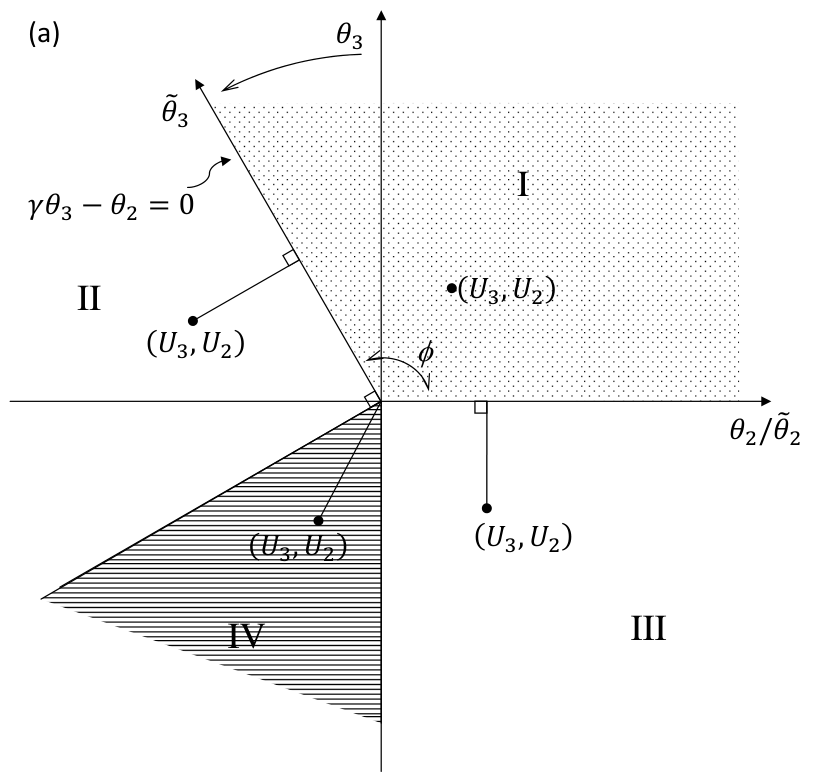
Now the parameter space is reduced to 2 dimensions. Under the orthonormal transformation, the cone spaces become to $\tilde{C}=\{\boldsymbol{\theta}:\gamma\theta_{3}-\theta_{2}\geq 0,\theta_{3}\geq 0\}$, and $\tilde{C}_{0}=\{\boldsymbol{\theta}:\theta_{3}=\theta_{2}=0\}$, where $\gamma=\tilde{\mathcal{I}}_{23}\cdot|\tilde{\mathcal{I}}(\boldsymbol{\theta}_{0})|^{-1/2}$ is the slope of the axis $\theta_{3}$ after transformation as shown in Figure 1(a). To account for the fact that $\theta_{1}$ is estimated, $\tilde{\mathcal{I}}(\boldsymbol{\theta}_{0})$ is defined from the $3\times 3$ information matrix $\mathcal{I}(\boldsymbol{\theta}_{0})$ as

From the graphic point of view, the representation of the test statistics (27) is determined by the minimum distance of the independent normal vector $U=(U_{2},U_{3})^{T}$ to $\boldsymbol{\theta}$. Under the alternative hypothesis, the minimum distance, $\inf_{\boldsymbol{\theta}\in\tilde{C}}\|U-\boldsymbol{\theta}\|^{2}$, can be understood as the projection of $U$ on the cone space $\tilde{C}$ when $U$ is outside of the cone. As shown in Figure 1(a), the representations of $\inf_{\boldsymbol{\theta}\in\tilde{C}}\|U-\boldsymbol{\theta}\|^{2}$ are different in the four regions of the plane with coordinates $(\theta_{2},\theta_{3})$

The area proportions, $(\phi,1/4,1/4,1/2-\phi)$ as in the aforementioned order, of these four regions determine the probabilities that the vector $U$ lies in which region, where $\phi=\cos^{-1}\left(\gamma\cdot(1+\gamma^{2})^{-1/2}\right)=\tilde{\mathcal{I}}_{23}\cdot(\tilde{\mathcal{I}}_{22}\tilde{\mathcal{I}}_{33})^{-1/2}$.

Under the null hypothesis, the parameters space is reduced to the origin of the plane, thus according to Vu and Zhou (1997)

Then the asymptotic distribution of $D$ is the difference of the above two representations

Note that because $U_{2}$ and $U_{3}$ are independent, thus $(\gamma U_{2}+U_{3})/\sqrt{1+\gamma^{2}}\sim N(0,1)$, and the final approximate asymptotic distribution of $D$ is

In this paper, we suppose $\lim_{n\rightarrow\infty}|\gamma|<\infty$. If $\lim_{n\rightarrow\infty}|\gamma|\rightarrow\infty$, the representation of $\inf_{\boldsymbol{\theta}\in\tilde{C}}\|U-\boldsymbol{\theta}\|^{2}$ is in different form (Vu and Zhou, 1997) and the asymptotic distribution of $D$ may be different. An additional approximation is that we obtain $\gamma$ with a finite sample size under the null hypothesis, so we assume that $n$ is large enough that the finite $\gamma$ is close to the converged value.

The RLRT for two variance components introduced above allows us to test the overall pathway effect. Furthermore, we may be attracted to testing single variance components, such as testing the P-E effect, given that the overall the pathway effect test is significant. The hypothesis of this problem is

which is equivalent to testing $H_{0}:\tau_{xz}=0$ vs. $H_{a}:\tau_{xz}>0$. The RLRT test statistics $d=2l_{PR}(\boldsymbol{\theta})-2l_{PR}(\boldsymbol{\theta}_{0})$ for one variance component in semiparametric model with PRL was also suggested by Claeskens (2004), and an exact RLRT algorithm was proposed by Crainiceanu et al. (2005). Unfortunately, this exact RLRT method cannot apply to test (31) for model (12). In their work, there are no random effects in the model under the null hypothesis, thus $d$ can be represented exactly as the form of a mixture of chi-square distribution. On the contrary, our model (12) under the null hypothesis of (31) contains two random effects $\mathbf{r}_{x}$ and $\mathbf{r}_{z}$, which makes it impossible to represent $d$ exactly.

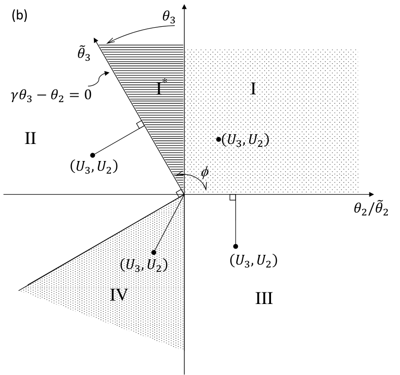
The second choice is to use the method described in the previous section using an asymptotic distribution. However, we need the same approximations; that is, we fix $\rho$ and assume that the relationship between the response and the environmental variable is almost linear, i.e. $\tau_{x}\approx 0$. Then similarly, the parameters cone space is reduced to 2 dimensions. One interesting parameter $\theta_{3}=\lambda^{-1}_{xz}$, and one nuisance parameter $\theta_{2}=\lambda_{z}^{-1}$, both have the true values on the boundary. Thus, $C_{\Omega}=[0,\infty)\times[0,\infty)$ and $C_{\Omega_{0}}=[0,\infty)\times\{0\}$.
Under the approximations described above, the asymptotic representation of 2 times the log PRL function under the null hypothesis is

where $I(\cdot)$ is the indicator function. The representation under the alternative hypothesis is the same as in (28), but because the cone under the null hypothesis is no longer the origin of the $(\theta_{2},\theta_{3})$ plane, $\inf_{\boldsymbol{\theta}\in\tilde{C}_{0}}\|U-\boldsymbol{\theta}\|^{2}$ has two regions as shown by (32). Now we must divide the plane with coordinates $(\theta_{2},\theta_{3})$ into five regions and set the approximated asymptotic representation of $d$ as (see Figure 1(b))

Thus, we have the asymptotic distribution of $d$ for testing $\theta_{3}=\lambda_{xz}^{-1}=0$ or $\tau_{xz}=0$

References

- Adami, et al. (2008) Adami, H. O., Hunter, D., and Trichopoulos, D. (2008). Textbook of Cancer Epidemiology. New York: Oxford University Press.
- Aronszajn (1950) Aronszajn, N. (1950). Theory of Reproducing Kernels, Transactions of the American Mathmatical Society, 68, 337-404.
- Benjamini and Hochberg (1995) Benjamini, Y. and Hochberg, Y. (1995). Controlling the False Discovery Rate: a Practical and Powerful Approach to Multiple Testing. Journal of the Royal Statistical Society, Series B, 57, 289-300.
- Breiman (1995) Breiman, L. (1995). Better Subset Regression Using the Nonnegative Garrote. Technometrics, 37, 373-384.
- Breslow and Clayton (1993) Breslow, N. E. and Clayton, D. G. (1993). Approximate Inference in Generalized Linear Mixed Models. Journal of the American Statistical Association, 88, 9-25.
- Chakravarti and Little (2003) Chakravarti, A. and Little, P. (2003). Nature, Nurture, and Human Disease. Nature, 421, 412-414.
- Chatterjee et al. (2006) Chatterjee, N., Kalaylioglu, Z., Moslehi, R., Peters, U., and Wacholder, S. (2006). Powerful Multilocus Tests of Genetic Association in the Presence of Gene-gene and Gene-environment Interactions. The American Journal of Human Genetics, 79, 1002-1016.
- Claeskens (2004) Claeskens, G. (2004). Restricted Likelihood Ratio Lack-of-fit Tests Using Mixed Spline Models. Journal of the Royal Statistical Society, Series B, 66, 909-926.
- Crainiceanu et al. (2005) Crainiceanu, C., Ruppert, D., Claeskens, G., and Wand, M. P. (2005). Exact Likelihood Ratio Tests for Penalized Splines. Biometrika, 92, 91-103.
- Czyzyk et al. (1989) Czyzyk, A., Lao, B., Orowska, K., Szczepanik, Z., and Bartosiewicz, W. (1989). Effect of Antidiabetics on Post-exercise Alaninemia in Patients with Non-insulin-dependent Diabetes Mellitus (Type 2). Polskie Archiwum Medycyny Wewntrznej, 81, 193-206.
- Franconi et al. (2006) Franconi, F., Loizzo, A., Ghirlanda, G., and Seghieri, G. (2006). Taurine Supplementation and Diabetes Mellitus. Current Opinion in Clinical Nutrition & Metabolic Care, 9, 32-36.
- Goeman et al. (2004) Goeman, J. J., van de Geer, S. A., de Kort F., and van Houwelingen, H. C. (2004). A Global Test for Groups of Genes: Testing Association with a Clinical Outcome. Bioinformatics, 20, 93-99.
- Goeman et al. (2005) Goeman, J. J., Oosting, J., Cleton-Jansen, A., Anninga, J. K., and van Houwelingen, H. C. (2005). Testing Association of a Pathway with Survival Using Gene Expression data. Bioinformatics, 21, 1950-1957
- Green (1987) Green, P. J. (1987). Penalized Likelihood for General Semi-parametric Regression Models. International Statistical Review, 55, 245-259.
- Green and Silverman (1994) Green, P. J. and Silverman, B. W. (1994). Nonparametric Regression and Generalized Linear Models. London: Chapman and Hall.
- Gu and Wahba (1993) Gu, C. and Wahba, G. (1993). Semiparametric Analysis of Variance with Tensor Product Thin Plate. Journal of the Royal Statistical Society, Series B, 55, 353-368.
- Guo (2002) Guo, W. (2002). Inference in Smoothing Spline Analysis of Variance. Journal of the Royal Statistical Society, Series B, 64, 887-898.
- Harville (1977) Harville, D. A. (1977). Maximum Likelihood Approaches to Variance Component Estimation and to Related Problems. Journal of the American Statistical Association, 72, 320-338.
- Hastie and Tibshirani (1990) Hastie, T. and Tibshirani, R. (1990). Generalized Additive Models. London; New York: Chapman and Hall.
- Hastie et al. (2009) Hastie, T., Tibshirani, R., and Friedman, J. (2009). The Elements of Statistical Learning: Data Mining, Inference, and Prediction. New York: Springer.
- Hahn et al. (2003) Hahn, L. W., Ritchie, M. D., and Moore, J. H. (2003). Multifactor Dimensionality Reduction Software for Detecting Gene-gene and Gene-environment Interaction. Bioinformatics, 19, 376-382.
- Jennrich and Schluchter (1986) Jennrich, R. J. and Schluchter, M. D. (1986). Unbalanced Repeated Measures Models with Structured Covariance Matrices. Biometrics, 42, 805-820.
- Juretić et al. (2002) Juretić, D., Krajnović, V., and Lukac-Bajalo, J. (2002). Altered Distribution of Urinary Glycosaminoglycans in Diabetic Subjects. Acta Diabetologica, 39, 123-8.
- Kim et al (2011) Kim, I., Pang, H., and Zhao, H. (2011). Semiparametric Methods for Evaluating Pathway Effects on Clinical Outcomes Using Gene Expression Data. Technical Report.
- Kimeldorf and Wahba (1971) Kimeldorf, G. and Wahba, G. (1971). Some Results on Tchebychefian Spline Functions. Journal of Mathematical Analysis and Applications, 33, 82-95.
- Lin (1997) Lin, X. (1997). Variance Component Testing in Generalized Linear Models with Random Effects. Biometrika, 84, 309-326.
- Lin and Zhang (1999) Lin, X. and Zhang, D. (1999). Inference in Generalized Additive Mixed Models by Using Smoothing Splines. Journal of the Royal Statistical Society, Series B, 61, 381-400.
- Liu et al (2008) Liu, D., Ghosh, D., and Lin, X. (2008). Estimation and Testing for the Effect of a Genetic Pathway on a Disease Outcome Using Logistic Kernel Machine Regression via Logistic Mixed Models. BMC Bioinformatics, 9, 292.
- Liu et al. (2007) Liu, D., Lin, X., and Ghosh, D. (2007). Semiparametric Regression of Multi-Dimensional Genetic Pathway Data: Least Squares Kernel Machines and Linear Mixed Models. Biometrics, 63, 1079-1088.
- MacKay (1998) MacKay, D. J. C. (1998). Introducing to Gaussian Process. In Bishop, C. M., editor, Neural Networks and Machine Learning. New York: Springer-Verlag.
- Maity et al. (2009) Maity, A., Carroll, R. J., Mammen, E., and Chatterjee, N. (2009). Testing in Semiparametric Models with Interaction, with Applications to Gene-environment Interactions. Journal of the Royal Statistical Society, Series B, 71, 75-96.
- Manolio et al. (2006) Manolio, T. A., Bailey-Wilson, J. E., and Collins, F. S. (2006). Genes, Environment and the Value of Prospective Cohort Studies. Nature Review Genetics, 7, 812-820.
- Misu et al. (2007) Misu, H., Takamura, T., Matsuzawa, N., Shimizu, A., Ota, T., Sakurai, M., Ando, H., Arai, K., Yamashita, T., Honda, M., Yamashita, T., and Kaneko, S. (2007). Genes Involved in Oxidative Phosphorylation are Coordinately Upregulated with Fasting Hyperglycaemia in Livers of Patients with Type 2 Diabetes. Diabetologia, 50, 268-277.
- Moore et al. (2010) Moore, J. H., Asselbergs, F. W., and Williams, S. M. (2010). Bioinformatics Challenges for Genome-wide Association Studies. Bioinformatics, 26, 445-455.
- Mootha et al. (2004) Mootha, V. K., Handschin, C., Arlow, D., Xie, X., Pierre, J. S., Sihag, S., Yang, W., Altshuler, D., Puigserver, P., Patterson, N., Willy, P. J., Schulman, I. G., Heyman, R. A., Lander, E. S., and Spiegelman, B. M. (2004). Err and Gabpa/b Specify PGC-1-dependent Oxidative Phosphorylation Gene Expression that is Altered in Diabetic Muscle. Proceedings of the National Academy of Sciences, 101, 6570-6575.
- Mootha et al. (2003) Mootha, V. K., Lindgren, C. M., Eriksson, K., Subramanian, A., Sihag, S., Lehar, J., Puigserver, P., Carlsson, E., Ridderstrale, M., Laurila, E., Houstis, N., Daly, M. J., Patterson, N., Mesirov, J. P., Golub, T. R., Tamayo, P., Spiegelman, B., Lander, E. S., Hirschhorn, J. N., Altshuler, D., and Groop, L. C. (2003). PGC-l alpha-Responsive Genes Involved in Oxidative Phosphorylation are Coordinately Downregulated in Human Diabetes. Nature Genetics, 34, 267-273.
- Pang et al. (2006) Pang, H., Lin, A., Holford, M., Enerson, B., Lu, B., Lawton, M. P., Floyd, E., and Zhao, H. (2006). Pathway Analysis Using Random Forests Classification and Regression. Bioinformatics, 22, 2028-2036.
- Pang and Zhao (2008) Pang, H. and Zhao, H. (2008). Building Pathway Clusters form Random Forest Classification Using Class Votes. BMC Bioinformatics, 9, 87.
- Pang et al. (2011) Pang, H., Kim, I., and Zhao, H. (2011). Random Effect Model for Multiple Pathway Analysis with Applications to Type II Diabetes Microarray Data. Technical Report.
- Park and Hastie (2008) Park, M. Y. and Hastie, T. (2008). Penalized Logistic Regression for Detecting Gene Interactions. Biostatistics, 9, 30-50.
- Rasmussen and Williams (2006) Rasmussen, C. E. and Williams, C. K. I. (2006). Gaussian Process for Machine Learning. Cambridge: MIT Press.
- Ritchie et al. (2001) Ritchie, M. D., Hahn, L. W., Roodi, N., Bailey, L. R., Dupont, W. D., Parl, F. F., and Moore, J. H. (2001). Multifactor-dimensionality Reduction Reveals High-order Interactions Among Estrogen-metabolism Genes in Sporadic Breast Cancer. The American Journal of Human Genetics, 69, 138-147.
- Tipping (2001) Tipping, M. E. (2001). Sparse Bayesian Learning and the Relevance Vector Machine. Journal of Machine Learning Research, 1, 211-244.
- Searle et al. (1992) Searle, S. R., Casella, G., and McCulloch, C. E. (1992). Variance Components. New York: Wiley.
- Simon et al. (2011) Simon, R., Marks, V., Leeds, A., and Anderson, J. (2011). A Comprehensive Review of Oral Glucosamine Use and Effects on Glucose Metabolism in Normal and Diabetic Individuals. Diabetes Metabolism Research and Reviews, 27, 14-27
- Storey (2002) Storey, J. D. (2002). A Direct Approach to False Discovery Rates. Journal of the Royal Statistical Society, Series B, 64, 479-498.
- Vu and Zhou (1997) Vu, H. T. V. and Zhou, S. (1997). Generalization of Likelihood Ration Tests under Nonstandard Conditions. Annals of Statistics, 25, 897-916.
- Wahba (1990) Wahba, G. (1990). Spline Models for Observational Data. Philadelphia: Society for Industrial and Applied Mathematics.
- Wang, et al. (2007) Wang, K., Li M., and Bucan, M. (2007). Pathway-based Approaches for Analysis of Genomewide Association Studies. The American Journal of Human Genetics, 81, 1278-1283.
- Zhang et al. (1998) Zhang, D., Lin, X., Raz, J., and Sowers, M. (1998). Semiparametric Stochastic Mixed Models for Longitudinal data. Journal of the American Statistical Association, 93, 710-719.
- Zhang and Lin (2003) Zhang, D. and Lin, X. (2003). Hypothesis Testing in Semiparametric Additive Mixed Models. Biostatistics, 4, 57-74.
- Zou et al. (2010) Zou, F., Huang, H., Lee, S., and Hoeschele, I. (2010). Nonparametric Bayesian Variable Selection with Applications to Multiple Quantitative Trait Loci Mapping with Epistasis and Gene-Environment Interaction. Genetics, 186, 385-394.