The purely singular 1-D acoustic reflection problem

The physical setup is as follows. Consider a three-dimensional acoustic medium with coordinates $(x,y,z)$ such that the medium varies only in the $z$-direction and such that the density $\rho(z)$ and bulk modulus $K(z)$ are piecewise constant with respect to $z$, having jumps at points

$$z_{0}<z_{1}<\cdots<z_{M},$$

where $M\geq 1$. Let $z_{-1}<z_{0}$ denote a fixed reference depth in the homogeneous half space $z<z_{0}$ from which signals in the form of traveling plane waves may be transmitted and received. In keeping with the geophysical perspective, the $z$-coordinate will be interpreted as depth, and it will be depicted as increasing downward, as in Figure 1.

The depth range $z_{n-1}<z<z_{n}$ with be referred to as the $n$th layer, for $1\leq n\leq M$. Thus there are $M$ layers and $M+1$ interfaces, the latter being located at depths $z_{0},z_{1},\ldots,z_{M}$.

Let $u(t,z)$ denote the velocity (in the $z$-direction) of a material particle at depth $z$ and time $t$, and let $p(t,z)$ denote the pressure. The medium evolves according to the coupled one-dimensional equations

	$\displaystyle\rho\frac{\partial u}{\partial t}+\frac{\partial p}{\partial z}$	$\displaystyle=0$		(1.1a)
	$\displaystyle\frac{1}{K}\frac{\partial p}{\partial t}+\frac{\partial u}{\partial z}$	$\displaystyle=0.$		(1.1b)

In analyzing the solution to the above system, there is a choice to be made between working with $u(t,z)$ or $p(t,z)$ (or a certain combination or the two). The situation is essentially the same whatever the choice; for the sake of definiteness the present article will focus on the velocity field $u(t,z)$, which is the quantity measured by a coil/magnet geophone, for instance. The initial conditions corresponding to a plane wave unit impulse propagating downward from $z_{-1}$ are

$$\begin{split}u(0,z)&=\delta(z-z_{-1})\\ p(0,z)&=\sqrt{K(z_{-1})\rho(z_{-1})}\;\delta(z-z_{-1}).\end{split}$$

(1.2)

Let $G(t)$ denote the (velocity) impulse response at $z_{-1}$, so that

$$G(t)=u(t,z_{-1})\quad\quad(t>0),$$

(1.3)

the solution at depth $z_{-1}$ to the system (1.1a,1.1b,1.2).

The work [8, Chapter 3] of Fouque et al. summarizes very clearly the standard theory concerning propogation of waves in a piecewise constant layered medium, including a derivation of the governing equations (1.1a,1.1b) from physical principles; it will serve as a principal reference. See [5, Section 2] for an alternate treatment of the same material. The following facts, proved in [8, Chapter 3] and elsewhere, serve as a starting point for the present paper. For $1\leq n\leq M$, let $\tau_{n}$ denote the two-way travel time (for a traveling wave) across the $n$th layer of the above $M$-layer medium, and let $\tau_{0}$ denote the two-way travel time from depth $z_{-1}$ to $z_{0}$. For $0\leq n\leq M$, let $R_{n}$ denote the reflection coefficient at depth $z_{n}$ relative to a wave traveling toward the interface from above. Letting $K_{n}$ and $\rho_{n}$ denote the density and bulk modulus inside the $n$th layer—with $K_{-1},\rho_{-1}$ and $K_{M+1},\rho_{M+1}$ denoting the respective values at $z_{-1}$ and any point $z_{M+1}$ below $z_{M}$—the travel times and reflectivities are given by the formulas

$$\tau_{n}=\frac{2(z_{n}-z_{n-1})}{\sqrt{K_{n}/\rho_{n}}}\quad\mbox{ and }\quad R_{n}=\frac{\sqrt{K_{n}\rho_{n}}-\sqrt{K_{n+1}\rho_{n+1}}}{\sqrt{K_{n}\rho_{n}}+\sqrt{K_{n+1}\rho_{n+1}}},$$

(1.4)

for $0\leq n\leq M$. Note that $-1<R_{n}<1$ by virtue of (1.4). Let $(\tau,R)$ denote the pair of sequences

$$\tau=(\tau_{0},\ldots,\tau_{M})\quad\mbox{ and }\quad R=(R_{0},\ldots,R_{M}),$$

and let $|\tau|$ denote the total two-way travel time from $z_{-1}$ to $z_{M}$,

$$|\tau|=\tau_{0}+\cdots+\tau_{M}.$$

The pair $(\tau,R)$ will be referred to as a model; it completely determines $G(t)$ and hence represents the underlying physical structure insofar as concerns the impulse response. To emphasize this dependence, the impulse response as defined in (1.3) will be denoted $G^{(\tau,R)}(t)$. Moreover, the impulse response has the structure of a delta train of the form

$$G^{(\tau,R)}(t)=\sum_{n=1}^{\infty}\alpha_{n}\delta(t-\sigma_{n}).$$

(1.5)

Without loss of generality the representation (1.5) will be taken to be in normal form, whereby each $\alpha_{n}\neq 0$ and the arrival times $\sigma_{n}$ are in their natural order,

$$\sigma_{1}<\sigma_{2}<\sigma_{2}<\cdots.$$

In practice the impulse response (1.5) can only be known for some finite time interval $[0,t_{\rm max}]$. If $t_{\rm max}<|\tau|$, say

$$\tau_{0}+\cdots+\tau_{N}\leq t_{\rm max}<\tau_{0}+\cdots+\tau_{N+1},$$

then the terms $\tau_{N+1},\ldots,\tau_{M}$ and $R_{N+1},\ldots,R_{M}$ have no influence on $G^{(\tau,R)}(t)$ for $t\in[0,t_{\rm max}]$. That is, letting $\tau^{\prime}=(\tau_{0},\ldots,\tau_{N})$ and $R^{\prime}=(R_{0},\ldots,R_{N})$,

$$G^{(\tau,R)}(t)=G^{(\tau^{\prime},R^{\prime})}(t)\mbox{ for }t<t_{\rm max}.$$

Thus one may as well study just $G^{(\tau^{\prime},R^{\prime})}$. Based on this reasoning, let $\chi_{[0,|\tau|]}$ denote the characteristic function of the finite interval $[0,|\tau|]$ and consider the partial impulse response

$$\chi_{[0,|\tau|]}G^{(\tau,R)}(t)=\sum_{n=1}^{d}\alpha_{n}\delta(t-\sigma_{n}).$$

(1.6)

Letting $(\sigma,\alpha)$ denote the finite sequences

$$\sigma=(\sigma_{1},\ldots,\sigma_{d})\mbox{ and }\alpha=(\alpha_{1},\ldots,\alpha_{d}),$$

the central problem of the present paper is to analyze the mapping

$$(\tau,R)\mapsto(\sigma,\alpha).$$

The data $(\sigma,\alpha)$ corresponding to (1.6) is well-defined provided that the right-hand side is in normal form, a convention that will be in force from now on.
Forward problem. Given an $M$-layer model $(\tau,R)$, for some $M\geq 1$, determine the data $(\sigma,\alpha)$ for which equation (1.6) holds. Inverse problem. Given the data $(\sigma,\alpha)$ such that equation (1.6) holds for an $M$-layer model $(\tau,R)$, for some $M\geq 1$, determine the model.
In the above formulation, the vectors $\tau$ and $R$ are arbitrary, in the sense that any

$$\tau\in\mathbb{R}^{M+1}_{>0}\quad\mbox{ and }\quad R\in(-1,1)^{M+1}$$

comprise a possible model, for any $M\geq 1$. Three features distinguish the above formulation, setting it apart from earlier treatments of the problem:

1. 1.

   the data is a delta train and hence purely singular;

2. 2.

   the $\tau_{n}$ are arbitrary—they need not all be equal;

3. 3.

   the data is restricted to finite time.

The purely singular structure fits the scenario of Candès and Fernandez-Granda’s work [6] on superresolution. Their results suggest that, within certain constraints, it may be possible to extract the function $\chi_{[0,|\tau|]}G^{(\tau,R)}(t)$ from measured data, which one expects to be a convolution of the form

$$\bigl(G^{(\tau,R)}\ast f\bigr)(t),$$

for some non-sigular wavelet $f(t)$. Deconvolution, which has its own long history, will not be considered in the present paper. While the purely singular structure is suited to superresolution, it is unsuited to classical methods such as that of Gelfand-Levitan, as pointed out by Bube and Burridge [5, Section 1.2]. The second item above, that the $\tau_{n}$ need not be equal, distinguishes the present formulation from several influential papers on the 1-D reflection problem, including that of Berryman-Goupillaud-Waters [2], Kunetz [11] and Bube-Burridge [5]. Each of the latter assumes constant travel times across layers, which turns out to change the problem substantially from the generic case in which travel times across layers are unrelated to one another. (See below for more on this point.) Lastly, the finite time restriction of item (3) makes frequency domain methods unsuitable if one is interested in exact formulas rather than series approximations. This motivates Browning’s work [4] on extrapolation, for example. Indeed series approximations underpin a range of approaches to the reflection problem, in both 1-D and higher. See the survey [21] for an overview based on the Lippmann-Scwinger equation, and [9] for more recent work along the same lines. The present paper avoids series approximations altogether.

The forward and inverse problems stated in Section 1.1 are solved completely, facilitating a precise description of the model-data correspondence. The picture that emerges will be sketched below, following some remarks on the forward problem. An explicit solution to the forward problem is stated in Theorem 2.1 and its corollories. The proof of the theorem—deferred to Section 6—entails a comprehesive analysis of scattering sequences, carried out by means of combinatorial arguments tailored specifically to the task. The resulting formulas have a very nice structure: the amplitudes $\alpha_{n}$ in the data turn out to be polynomial functions of the reflectivity $R$. These polynomials are homogeneous, have integer coefficients, and are consequently easy to code up. The arrival times $\sigma_{n}$ have an even simpler structure. Thus the solution to the forward problem leads to a straightforward exact algorithm, Algorithm 5.1.

It is proved in Section 3 that the mapping from models to data is not globally injective; distinct models of differing dimensions can produce the same data as one another. This ill-posedness is shown to to stem from alignment of the travel time vector $\tau=(\tau_{0},\ldots,\tau_{M})$ with the integer lattice $\mathbb{Z}^{M+1}$, such as when the $\tau_{n}$ are all equal—a basic assumption of numerous papers on the 1-D problem! The ill-posedness is remedied by discarding a small set of models (having measure zero in each dimension). As shown in Corollary 4.3, the mapping from models to data is injective on the remainder, which are referred to as generic models.

More than this, the set of $M$-layer generic models is naturally partitioned into open sets $X_{\psi}$. On each set, the mapping $(\tau,R)\mapsto(\sigma,\alpha)$ is given by a fixed formula, which has the following form. Viewing $\tau$ and $\sigma$ as row vectors, there is an integer matrix $A_{\psi}$ (Definition 4.3) such that

$$\sigma=\tau A_{\psi}$$

(1.7)

(valid throughout $X_{\psi}$). And each amplitude $\alpha_{n}$ has the form $p_{\psi,n}(R)$ (also valid throughout $X_{\psi}$), where $p_{\psi,n}$ is an explicitly given multivariate polynomial determined by $\psi$. Thus within each $X_{\psi}$ the mapping decouples into two independant maps $\tau\mapsto\sigma$ and $R\mapsto\alpha$. The integer matrix $A_{\psi}$ and the polynomials $p_{\psi,n}$ change from one open set $X_{\psi}$ to another. In fact, the integer matrix $A_{\psi}$ is an invariant that uniquely labels $X_{\psi}$ and determines the associated polynomials $p_{\psi,n}$. The mapping from generic models to data is a diffeomorphism on each $X_{\psi}$, and it is globally injective when $X_{\psi}$ ranges over all possible $M$. See Theorem 4.1.

Concerning the inverse problem, the discrete invariant $A_{\psi}$ can be computed directly from the arrival time data $\sigma$, where $(\sigma,\alpha)$ is the data corresponding to some $(\tau,R)\in X_{\psi}$. In practice the travel time vector $\tau$ and the matrix $A_{\psi}$ are simultaneously extracted from $\sigma$—see Algorithm 5.2. The matrix $A_{\psi}$ then serves as a pointer, indicating which formulas $p_{\psi,n}(R)$ are associated with which amplitudes $\alpha_{n}$. This allows one to pick out the amplitudes of primary reflections, which have the simplest formulas, and from which the reflection coefficients $R_{n}$ may be rapidly computed. Crucially, it also allows one to cross-check the reflection coefficients using the amplitudes of multiple reflections (a hugely redundant source) making it possible to correct amplitudes that may have been distorted. The idea is implemented in Algorithm 5.3. An important feature of the inverse algorithm (Algorithm 5.2), which depends on the irregular structure of generic models, is that it sequentially solves for $\tau$ from $\sigma$ and then for $R$ from $\alpha$. (With one extra piece of data it is possible to solve the inverse problem for non-generic data, but the algorithm does not decouple as in the generic case and is therefore much slower.)

This is not to say that the inverse problem can be solved in a practical way without limitation. On the contrary, there is a simple geometric way to interpret the formula (1.7) as a projection of lattice points that shows that for any precision $\varepsilon$, there are orientations of the vector $\tau$ (and hence associated $\psi$) for which successive entries in the arrival time data $\sigma$ will be separated by less than $\varepsilon$, rendering practical computation impossible. See Section 2.3.

The key results in the present paper are: the explicit form of the amplitude polynomials $p_{\psi,n}$ (Theorem 2.1), the decoupled inverse algorithm (Algorithms 5.2 and 5.3), and the characterization of the mapping from models to data as locally linear/polynomial and globally injective (Theorems 4.1 and 4.2).

Newton’s paper [15] surveys literature on the reflection problem up to 1980. Apart from the papers cited already in previous sections, notable results since 1980 include those of Santosa-Schwetlick [16] and Santosa-Symes [17]. The past two decades have seen considerable progress in the study of scaling limits for randomly layered media, and time reversal methods. The book [8] by Fouque et al. systematically covers the latter topics, which may be broadly characterized as stochastic. By contrast, the present paper, while starting with the same layered medium as in [8], takes an entirely deterministic approach—and the analysis is entirely in the time domain.

The non-negative integer lattice $\mathbb{Z}^{M+1}_{\geq 0}$ plays a central role in the analysis of an $M$-layer model $(\tau,R)$; fix notation as follows. A point $k\in\mathbb{Z}^{M+1}$ will be indexed starting with 0,

$$k=(k_{0},k_{1},\ldots,k_{M}),$$

consistent with the convention for models. For lattice points $k,k^{\prime}\in\mathbb{Z}^{M+1}$, the notation $k\leq k^{\prime}$ refers to the entrywise comparison of vectors,

$$k\leq k^{\prime}\mbox{ if and only if }k_{n}\leq k^{\prime}_{n}\mbox{ for each }0\leq n\leq M.$$

(This will be referred to as the natural partial order on $\mathbb{Z}^{M+1}$.) By the same token, the minimum of a pair of lattice points is to be interpreted entrywise,

$$\min\{k,k^{\prime}\}=\bigl\{\min\{k_{0},k^{\prime}_{0}\},\ldots,\min\{k_{M},k^{\prime}_{M}\}\bigr\}.$$

The symbol $\mathbb{1}\in\mathbb{Z}^{M+1}$ indicates the vector of ones,

$$\mathbb{1}=(1,1,\ldots,1),$$

and for $0\leq n\leq M$, the symbol $k^{n}$ denotes the vector consisting of $n+1$ ones followed by $M-n$ zeros,

$$k^{n}_{j}=\left\{\begin{array}[]{cl}1&\mbox{ if }0\leq j\leq n\\ 0&\mbox{ if }n+1\leq j\leq M\end{array}.\right.$$

(2.1)

So in particular $k^{M}=\mathbb{1}$ and $k^{0}=(1,0,\ldots,0)$; the lattice points $k^{0},\ldots,k^{M}$ are called primary vectors.

(The term “transit count vector” is a reference to scattering sequences; see Section 6.) Note that the lattice set $\mathfrak{L}^{\tau}_{M}$ of a travel time sequence is a finite set of lattice points, containing each of the primary vectors $k^{0},\ldots,k^{M}$. The notion of lattice set induces an equivalence relation on travel time sequences: declare $M$-layer travel time sequences $\tau$ and $\tau^{\prime}$ equivalent if $\mathfrak{L}^{\tau}_{M}=\mathfrak{L}^{\tau^{\prime}}_{M}$. The equivalence relation for $M=3$ is depicted in Figure 3 of Section 3.2.

The following (standard) multi-index notation helps to simplify some needed formulas. Give a vector $x=(x_{0},\ldots,x_{M})$ and a lattice point $k\in\mathbb{Z}^{M+1}$, $x^{k}$ denotes the monomial

$$x^{k}=\prod_{n=0}^{M}x_{n}^{k_{n}}.$$

And given lattice points $b,k\in\mathbb{Z}^{M+1}$ with $0\leq b\leq k$, the multi-index binomial coefficient $\binom{k}{b}$ is defined by the formula

$$\binom{k}{b}=\prod_{n=0}^{M}\binom{k_{n}}{b_{n}}=\prod_{n=0}^{M}\frac{k_{n}!}{b_{n}!(k_{n}-b_{n})!}.$$

The following propositions record properties and examples of amplitude polynomials that will be needed later. Observe that $a(x,k)$ has degree $2|k|-1$ and is homogenous with respect to the $2M+1$ variables $x_{0},\ldots,x_{M},y_{0},\ldots,y_{M-1}$. (Since $b\leq\tilde{k}$ the variable $y_{M}$ does not occur.) Homogeneity and odd degree imply that amplitude polynomials are odd, as follows.

The following connection between amplitude polynomials of differing numbers of variables is immediate from the definition.

Thus an amplitude polynomial $a(x,k)$ depends only on the non-zero entries $k_{n}$ of $k$ and the corresponding variables $x_{n}$. An important special case is that of primary vectors $k^{n}$, as defined above by (2.1).

A second example serves to illustrate how amplitude polynomials relate to one another when their respective transit count vectors differ in a single entry. Fix notation as follows: for $0\leq n\leq M$, let $e^{n}$ denote the standard basis vector in $\mathbb{Z}^{M+1}$, whose entries are

$$e^{n}_{j}=\left\{\begin{array}[]{cl}1&\mbox{ if }j=n\\ 0&\mbox{ if }\quad j\neq n\end{array}.\right.$$

The impulse response may be expressed in terms of the underlying model using the amplitude polynomials of Definition 2.2, as follows.

The proof of the theorem is postponed to Section 6. The simplicity of this result is remarkable—yet it is apparently new. Restricting the sum (2.4) to the lattice set for $\tau$ adapts the result to the finite time interval $0\leq t\leq|\tau|$, as follows.

Thus the data $(\sigma,\alpha)$ corresponding to a given model $(\tau,R)$ is obtained by putting the right-hand side of (2.5) in normal form, thereby solving the forward problem. It will be useful to formalize this procedure by introducing an explicit mapping, in order to distinguish some fundamentally different cases.

The enumeration function $\psi=\Psi(\tau,R)$ need not be injective; in general it induces a partial ordering $\preceq$ on the lattice set $\mathfrak{L}^{\tau}_{M}$ according to the prescription

$$\forall k,k^{\prime}\in\mathfrak{L}^{\tau}_{M},\quad k\preceq k^{\prime}\Longleftrightarrow\psi(k)\leq\psi(k^{\prime}).$$

(2.6)

The data for a given model may be expressed in terms of the model with the aid of its enumeration function as follows.

This solves the forward problem completely.

There is a simple geometric interpretation of the arrival times $\sigma_{n}$ in the typical case where $\psi$ is non-zero. Up to rescaling, arrival times are essentially the orthogonal projection of the positive octant of the $M+1$-dimensional integer lattice onto a line having direction vector $\tau$. More precisely, they are a rescaling of the projection of the lattice set $\mathfrak{L}^{\tau}_{M}$ onto the line with direction vector $\tau$. This can be sketched in low dimensions; as an illustration, consider the 3-layer case

$$\tau=(1,0.327971,0.152455,1.51957).$$

Except for the vector $k^{3}=(1,1,1,1)$, each member of $\mathfrak{L}^{\tau}_{3}$ lies in a two-dimensional plane in $\mathbb{Z}^{4}$. See Figure 2.

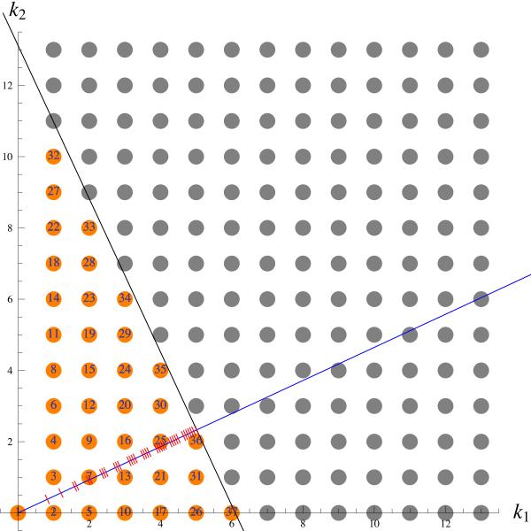
For this particular choice of $\tau$, the numbers $\sigma_{n}$ corresponding to arrival time data are depicted in Figure 2 as the orthogonal projection (red dashes) of the orange points onto the blue line. The blue line is the orthogonal projection of $\tau$ onto the $(k_{1},k_{2})$-plane. Later arrival times would correspond to projections of the gray points. The numbering of the orange points indicates the values of the enumeration function $\psi$, which will be shown later to be a locally constant function of $\tau$.

This view of arrival times as the orthogonal projection of lattice points onto a line explains both their pattern and density with increasing time. It is closely related to the cut-and-project construction of quasicrystals due to Kramer and Neri [10]. In this connection see [1] and also [7], who traces lattice projections back to the almost periodic functions of Bohr [3]. Note that for layered media the link to almost periodicity has a direct manifestation: the Fourier transform $\widehat{G^{(\tau,R)}}(\omega)$ of the impulse response is an almost periodic function in the sense of Bohr. Returning to present considerations, as long as the direction of the line determined by $\tau$ is not rational, arrival times will be aperiodic and eventually arbitrarily dense. On the other hand, the periodic structure of arrival times associated with, for example, a Bragg mirror, corresponds to a rational choice of $\tau$ that lines up with the lattice.

The mapping $(\tau,R)\mapsto(\sigma,\alpha)$ taking a model to its data is not injective, as the following example illustrates.

Let $\psi=\Psi(\tau,R)$, the enumeration function for the above $2$-layer model. Notice that

$$\psi\bigl((1,2,0)\bigr)=\psi\bigl(k^{2})=0.$$

So $\psi$ both takes the value zero and fails to be injective. Example 3.1 is part of a general pattern; similar examples exist in every higher dimension. The following technical lemma captures the essential reason.

Many of the historical approaches to the 1-D seismic problem make a simplifying assumption that the travel time vector $\tau$ is constant. But constant $\tau$ are easily seen to satisfy the hypothesis of Lemma 3.2. It follows from this that the inverse problem for such models is ill-posed.

What about non-constant travel time vectors? After all, a randomly chosen $M$-layer travel time vector will not be constant. (In fact, with probability one, it’s entries will be linearly independent over the rational numbers.)

A starting point is to consider travel time vectors that satisfy the hypothesis of Lemma 3.2, since this is the source of the ill-posedness expressed in Theorem 3.1. The case of $3$-layer travel time vectors $\tau=(\tau_{0},\tau_{1},\tau_{2},\tau_{3})$ illustrates the general situation. Observe that a transit count vector $k\in\mathfrak{L}^{\tau}_{M}$ different from $k^{3}$ satisfies $\langle k,\tau\rangle=\langle k^{3},\tau\rangle$ if and only if

$$(k_{1}-1)\hat{\tau}_{1}+(k_{2}-1)\hat{\tau}_{2}-\hat{\tau_{3}}=0,\quad\mbox{ where }\hat{\tau}=\textstyle\frac{1}{\tau_{1}+\tau_{2}+\tau_{3}}(\tau_{1},\tau_{2},\tau_{3}).$$

(3.2)

Thus the normalized subvector $\hat{\tau}$ determines whether a given $3$-layer transit vector $\tau$ satisfies the hypothesis of Lemma 3.2. Of course $\hat{\tau}$ is a point in the standard two dimensional simplex $\Delta_{2}$, which is a triangle. Each $k\in\mathfrak{L}_{3}$ determines a line segment in $\Delta_{2}$ defined by the equation (3.2). The set of all such lines is plotted in Figure 3. The vertices, clockwise from the top, are $\hat{\tau}=(0,0,1),(0,1,0)$ and $(1,0,0)$. The union of lines represents the set of transit count vectors that satisfy the hypothsis of Lemma 3.2, so the lemma fails to hold on the complement. The cells bounded by the lines represent the set of all travel time vectors that have a given lattice set, in the sense that $\mathfrak{L}_{3}^{\tau}$ is constant for $\hat{\tau}$ ranging over a single cell—with distinct cells corresponding to distinct lattice sets. The bottom left triangular cell represents the set of travel time vectors $\tau$ such that $\mathfrak{L}_{2}^{\tau}=\bigl\{k^{0},k^{1},k^{2},k^{3}\bigr\}$, the minimum possible. Moving to the right, each successive cell adds a vector of the form $k=(1,n,0,0)$, with $n$ increasing from $2$ to $\infty$. Moving upward from the lower left, each successive cell adds a vector of the form $(1,1,n,0)$.

A zoomed image from the upper part of the triangle is depicted in Figure 4.

Of course there is a corresponding construction in every higher dimension. In general, for $M$-layer travel time vectors, the triangle $\Delta_{2}$ becomes a standard $(M-1)$-dimensional simplex $\Delta_{M-1}$, lines become hyperplanes, and polygonal cells become convex polytopes. Lemma 3.2 fails on the interior of each of the convex polytopes.

Thus in general Lemma 3.2 only holds on a set of $M$-layer travel time vectors of measure zero in $\mathbb{R}^{M+1}_{>0}$; this set happens to include constant travel time vectors. The idea of the next section is to recover injectivity of the mapping from models to data by excluding a thin set of models which encompasses all those whose travel time vectors satisfy the hypothesis of Lemma 3.2.

Thus if $(\tau,R)$ is generic, then its enumeration function $\psi=\Psi(\tau,R)$ has an inverse,

$$\varphi=\psi^{-1}:\{1,\ldots,d\}\mapsto\mathfrak{L}^{\tau}_{M}.$$

(4.1)

Here is an alternate characterization that follows directly from Defintion 2.3.

It will be useful to refer to the reflectivity sequences that satisfy property (2) of Proposition 4.1, and furthermore to have a notation for the set of travel time vectors associated to a common enumeration function.

Observe that $\tau^{\prime}\in U_{\psi}$ only if both $\mathfrak{L}^{\tau^{\prime}}_{M}=\mathfrak{L}^{\tau}_{M}$ and condition (1) of Proposition 4.1 holds. More than this,

As in Section 3.2, the case $M=3$ serves to illustrate the general situation. Proposition 4.1 implies that the question of whether or not a given

$$\tau=(\tau_{0},\ldots,\tau_{3})\in\mathbb{R}^{4}_{>0}$$

is generic depends only on the normalized vector

$$\hat{\tau}=\textstyle\frac{1}{\tau_{1}+\tau_{2}+\tau_{3}}(\tau_{1},\tau_{2},\tau_{3}).$$

In detail, $\tau$ fails to be generic if and only if there exist $k,k^{\prime}\in\mathfrak{L}_{3}$ such that

	$\displaystyle\langle(k_{1},k_{2},k_{3}),$	$\displaystyle\hat{\tau}\rangle\leq\langle\mathbb{1},\hat{\tau}\rangle,\quad\quad\langle(k^{\prime}_{1},k^{\prime}_{2},k^{\prime}_{3}),\hat{\tau}\rangle\leq\langle\mathbb{1},\hat{\tau}\rangle$		(4.2a)
	and	$\displaystyle\langle(k_{1}-k^{\prime}_{1},k_{2}-k^{\prime}_{2},k_{3}-k^{\prime}_{3}),\hat{\tau}\rangle=0.$		(4.2b)

Note that the two inequalities (4.2a) simply express that $k,k^{\prime}\in\mathfrak{L}^{\tau}_{3}$. The particular case where $k\in\mathfrak{L}^{\tau}_{3}$ and $k^{\prime}=k^{3}$ reduces to equation (3.2). Therefore the set of $\hat{\tau}$ that satisfy (4.2) for some $k,k^{\prime}\in\mathfrak{L}_{3}$ is a superset of the line segments plotted in Figure 3. The full set of solutions is plotted in Figure 5, with the additional segments coloured orange. The sets $U_{\psi}$ are the travel time vectors $\tau$ that correspond to the interiors of the cells in this figure.

A zoomed image from the upper part of the triangle is depicted in Figure 6.

A similar picture exists in every higher dimension. Thus in general, $U_{\psi}$ is the interior of the postive cone over a convex polytope crossed with $\mathbb{R}_{>0}$. The important point is that $U_{\psi}$ is a convex open neighbourhood of $\tau$, and such neighbourhoods partition the set of all travel time vectors belonging to generic models.

As for reflectivities, given a fixed $\psi=\Psi(\tau,R)$, Proposition 4.1 asserts that the vectors $R^{\prime}\in(-1,1)^{M+1}$ excluded from $\mathcal{R}_{\psi}$ are precisely those satisfying a polynomial equation of the form

$$a(R^{\prime},k)=0\quad\mbox{ for some }\quad k\in\mathfrak{L}^{\tau}_{M}.$$

Thus $\mathcal{R}_{\psi}$ is the complement of a finite union of algebraic hypersurfaces in $(-1,1)^{M+1}$. In particular, $\mathcal{R}_{\psi}$ is open and has full measure.

The enumeration function for a generic model may be represented as a matrix, as follows.

Note that since each of the primary vectors $k^{0},\ldots,k^{M}$ belongs to $\mathfrak{L}^{\tau}_{M}$, the matrix

$$K_{M}=\Bigl((k^{0})^{T}\;\;(k^{1})^{T}\;\cdots\;(k^{M})^{T}\Bigr)=\left(\begin{array}[]{ccccc}1&1&1&\cdots&1\\ 0&1&1&\cdots&1\\ 0&0&1&\cdots&1\\ \vdots&\vdots&\ddots&\ddots&\vdots\\ 0&0&\cdots&0&1\end{array}\right)$$

(4.3)

is a submatrix of $A_{\psi}$. Therefore $A_{\psi}$ has rank $M+1$. For future reference, let $J_{M}$ denote the inverse of $K_{M}$,

$$J_{M}=K_{M}^{-1}=\left(\begin{array}[]{cccccc}1&-1&0&0&\cdots&0\\ 0&1&-1&0&\cdots&0\\ 0&0&1&-1&\ddots&\vdots\\ 0&0&0&1&\ddots&0\\ \vdots&\vdots&\vdots&\ddots&\ddots&-1\\ 0&0&0&\cdots&0&1\end{array}\right).$$

(4.4)

The notation developed in the previous section sets the stage for a very simple description of the correspondence between a generic model and its data.

References

- [1] M. Baake and R. V. Moody. Self-similarities and invariant densities for model sets. In Algebraic methods in physics (Montréal, QC, 1997), CRM Ser. Math. Phys., pages 1–15. Springer, New York, 2001.
- [2] L. H. Berryman, P. L. Goupillaud, and K. H. Waters. Reflections from multiple transition layers part I—theoretical results. Geophysics, 23(2):223–243, 1958.
- [3] H. Bohr. Zur Theorie der fastperiodischen Funktionen. Acta Math., 47(3):237–281, 1926. III. Dirichletentwicklung analytischer Funktionen.
- [4] B. L. Browning. Time and frequency domain scattering for the one-dimensional wave equation. Inverse Problems, 16(5):1377–1403, 2000.
- [5] K. P. Bube and R. Burridge. The one-dimensional inverse problem of reflection seismology. SIAM Rev., 25(4):497–559, 1983.
- [6] E. J. Candès and C. Fernandez-Granda. Towards a mathematical theory of super-resolution. arXiv:1203.5871v1 [cs.IT], 42 pages, 8 figures.
- [7] S. Favorov. Bohr and Besicovitch almost periodic discrete sets and quasicrystals. Proc. Amer. Math. Soc., 140(5):1761–1767, 2012.
- [8] J.-P. Fouque, J. Garnier, G. Papanicolaou, and K. Sølna. Wave propagation and time reversal in randomly layered media, volume 56 of Stochastic Modelling and Applied Probability. Springer, New York, 2007.
- [9] K. A. Innanen. Born series forward modelling of seismic primary and multiple reflections: an inverse scattering shortcut. Geophysical Journal International, 177(3):1197–1204, 2009.
- [10] P. Kramer and R. Neri. On periodic and nonperiodic space fillings of obtained by projection. Acta Cryst. Sect. A, 40(5):580–587, 1984.
- [11] G. Kunetz. Quelques exemples d’analyse d’enregistrements sismiques. Geophysical Prospecting, 11(4):409–422, 1963.
- [12] D. Kurrant and E. Fear. An improved technique to predict the time-of-arrival of a tumor response in radar-based breast imaging. Biomedical Engineering, IEEE Transactions on, 56(4):1200 –1208, april 2009.
- [13] J.-F. Le Gall. Random trees and applications. Probab. Surv., 2:245–311, 2005.
- [14] A. E. Malcolm, B. Ursin, and M. V. De Hoop. Seismic imaging and illumination with internal multiples. Geophysical Journal International, 176(3):847–864, 2009.
- [15] R. G. Newton. Inversion of reflection data for layered media: a review of exact methods. Geophysical Journal of the Royal Astronomical Society, 65(1):191–215, 1981.
- [16] F. Santosa and H. Schwetlick. The inversion of acoustical impedance profile by methods of characteristics. Wave Motion, 4(1):99–110, 1982.
- [17] F. Santosa and W. W. Symes. Reconstruction of blocky impedance profiles from normal-incidence reflection seismograms which are band-limited and miscalibrated. Wave Motion, 10(3):209–230, 1988.
- [18] R. P. Stanley. Enumerative combinatorics. Vol. 2, volume 62 of Cambridge Studies in Advanced Mathematics. Cambridge University Press, Cambridge, 1999. With a foreword by Gian-Carlo Rota and appendix 1 by Sergey Fomin.
- [19] W. W. Symes. The seismic reflection inverse problem. Inverse Problems, 25(12):123008, 39, 2009.
- [20] G. Van Groenestijn and D. Verschuur. Using surface multiples to estimate primaries by sparse inversion from blended data. Geophysical Prospecting, 59(1):10–23, 2011.
- [21] A. B. Weglein, F. V. Araújo, P. M. Carvalho, R. H. Stolt, K. H. Matson, R. T. Coates, D. Corrigan, D. J. Foster, S. A. Shaw, and H. Zhang. Inverse scattering series and seismic exploration. Inverse Problems, 19(6):R27–R83, 2003.
- [22] T. Williams, E. Fear, and D. Westwick. Tissue sensing adaptive radar for breast cancer detection-investigations of an improved skin-sensing method. Microwave Theory and Techniques, IEEE Transactions on, 54(4):1308 – 1314, june 2006.
- [23] O. Yilmaz. Seismic data analysis : processing, inversion, and interpretation of seismic data. Number 10 in Investigations in Geophysics. Society of Exploration Geophysicists, Tulsa, OK, 2nd edition, 2001. Edited by Stephen M. Doherty.