Combinatorial degree bound for toric ideals of hypergraphs

The edge subring of a hypergraph $H$ is the monomial subalgebra parametrized by the edges of $H$. We derive a general degree bound for the minimal generators of its defining ideal, $I_{H}$, in terms of the structure of the underlying hypergraph.

Let $H$ be a hypergraph on $V=\{1,\dots,n\}$ with edge set $E$. Each edge $e_{i}\in E$ of size $d$ encodes a squarefree monomial $x^{e_{i}}:=\prod_{j\in e_{i}}x_{j}$ of degree $d$ in the polynomial ring $k[x_{1},\dots,x_{n}]$. The edge subring of the hypergraph $H$, denoted by $k[H]$, is the following monomial subring:

The toric ideal of $k[H]$, denoted $I_{H}$, is the kernel of the monomial map $\phi_{H}:k[t_{e_{i}}]\to k[H]$ defined by $\phi_{H}(t_{e_{i}})=x^{e_{i}}$. The ideal $I_{H}$ encodes the algebraic relations among the edges of the hypergraph. For the special case where $H$ is a graph, generating sets of the toric ideal of $k[H]$ have been studied combinatorially in [12, 13], [15], [19], and [20, 21].

The motivation for studying toric ideals $I_{H}$ is threefold. First, explicit results that relate $I_{H}$ to combinatorial properties of $H$ have existed only for graphs. Second, $I_{H}$ is related to the Rees algebra $\mathcal{R}(\mathcal{I}(H))$ of the edge ideal of $H$: in case when $H$ is a graph, the presentation ideal of $\mathcal{R}(\mathcal{I}(H))$ is completely determined by generators of $I_{H}$ and the syzygies of the edge ideal $\mathcal{I}(H)$. Third, these toric ideals correspond to Markov bases for algebraic statistical models; this connection is outlined at the end of the Introduction. A starting point of our work is the fact that combinatorial signatures of generators of $I_{H}$ are balanced edge sets of $H$. Balanced edge sets on uniform hypergraphs were introduced in [14], and are referred to as monomial walks.

This paper is based on the fact that the ideal $I_{H}$ is generated by binomials $f_{\mathcal{E}}$ arising from primitive balanced edge sets $\mathcal{E}$ of ${H}$ (See Proposition 3.1, a generalization of [14, Theorem 2.8]). A balanced edge set of $H$ is a multiset of bicolored edges $\mathcal{E}=\mathcal{E}_{blue}\sqcup\mathcal{E}_{red}$ satisfying the following balancing condition: for each vertex $v$ covered by $\mathcal{E}$, the number of red edges containing $v$ equals the number of blue edges containing $v$, that is,

A binomial $f_{\mathcal{E}}$ arises from $\mathcal{E}$ if it can be written as

Note that while $H$ is a simple hypergraph (it contains no multiple edges), $\mathcal{E}$ allows repetition of edges. In addition, the balanced edge set $\mathcal{E}$ is primitive if there exists no other balanced edge set $\mathcal{E}^{\prime}=\mathcal{E}^{\prime}_{blue}\sqcup\mathcal{E}^{\prime}_{red}$ such that $\mathcal{E}^{\prime}_{blue}\subsetneq\mathcal{E}_{blue}$ and $\mathcal{E}^{\prime}_{red}\subsetneq\mathcal{E}_{red}$; this is the usual definition of an element in the Graver basis of $I_{H}$. If $H$ is a uniform hypergraph, a balanced edge set is called a monomial walk to conform with the terminology in [20, 21] and [14].

In what follows, we give two general degree bounds for generators of $I_{H}$ (Section 5), study the combinatorics of splitting sets and reducibility (defined in Section 3), and explore implications to algebraic statistics throughout. Section 4 focuses on indispensable binomials, i.e. binomials that are members of every minimal generating set of $I_{H}$. Proposition 4.1 gives a combinatorial sufficient condition for determining whether a binomial $f\in I_{H}$ is indispensable. Consequently, the Graver basis is the unique minimal generating set of $I_{H}$ for any $2$-regular hypergraph (Proposition 4.2). In particular, this means that the Graver basis is equal to the universal Gröbner basis, although the defining matrix need not be unimodular.

Theorem 5.1 is a combinatorial criterion for the ideal of a uniform hypergraph to be generated in degree at most $d\geq 2$. The criterion is based on decomposable balanced edge sets, separators, and splitting sets; see Definitions 3.2 and 3.3. Our result generalizes the well-known criterion for the toric ideal of a graph to be generated in degree $2$ from [12] and [20, 21]. Splitting sets translate and extend the constructions used in [12] and [20, 21] to hypergraphs and arbitrary degrees. Theorem 5.3 provides a more general result for non-uniform hypergraphs.

In algebraic statistics, any log-linear statistical model corresponds to a toric variety whose defining ideal gives a Markov basis for the model (cf. Fundamental Theorem of Markov bases [6], [8]). Since these varieties, by definition, have a monomial parametrization, we can also associate to any log-linear model $\mathcal{M}$ with a square-free parameterization a (non-uniform) hypergraph $H_{\mathcal{M}}$. By Proposition 3.1, Markov moves for the model $\mathcal{M}$ are described by balanced edge sets of $H_{\mathcal{M}}$: if $\mathcal{E}$ is a balanced edge set of $H_{\mathcal{M}}$, then a Markov move on a fiber of the model corresponds to replacing the set of red edges in $\mathcal{E}$ by the set of blue edges in $\mathcal{E}$. Our degree bounds give a bound for the Markov complexity (Markov width) of the model $\mathcal{M}$. For general references on Markov complexity of classes for some log-linear models, the reader should refer to [4], [5], [8, Chapter 1, §2] and [10].

We apply our combinatorial criteria to recover a well-known result in algebraic statistics from [4] in Corollary 4.8. Finally, we study the Markov complexity of a set of models from [18] called hidden subset models. Namely, Theorem 5.6 says that the ideal associated to the image of $\Tan(({\mathbb{P}}^{1})^{n})$ in higher cumulants is generated by quadratics and cubics.

We remind the reader that all hypergraphs in this paper are simple, that is, they contain no multiple edges. In contrast, balanced edge sets of hypergraphs are not, since the binomials arising from the sets need not be squarefree. Therefore, for the purpose of this manuscript, we will refer to a balanced edge set as a multiset of edges, with implied vertex set; and, as usual, $V(\mathcal{E})$ denotes the vertex set contained in the edges in $\mathcal{E}$.

For the remainder of this short section, we will clear the technical details and notation we need for the proofs that follow.

A multiset, $M$, is an ordered pair $(A,f)$ such that $A$ is a set and $f$ is a function from $A$ to ${\mathbb{N}}_{>0}$ that records the multiplicity of each of the elements of $A$. For example, the multiset $M=(\{1,2\},f)$ with $f(1)=1$ and $f(2)=3$ represents $M=\{1,2,2,2\}$ where ordering doesn’t matter. We will commonly use the latter notation.

Given a multiset $M=(A,f)$, the support of $M$ is $\supp(M):=A$, and its size is $|M|:=\sum_{a\in A}f(a)$. For two multisets $M_{1}=(A,f_{1})$ and $M_{2}=(B,f_{2})$, we say $M_{2}\subseteq M_{1}$ if $B\subseteq A$ and for all $b\in B$, $f_{2}(b)\leq f_{1}(b)$. $M_{2}$ is a proper submultiset of $M_{1}$ if $B\subsetneq A$, or there exists a $b\in B$ such that $f_{2}(b)<f_{1}(b)$.

Unions, intersections, and relative complements of multisets are defined in the canonical way:

Note that the support of the union (intersection) of two multisets is the union (intersection) of their supports. Finally, we define a sum of $M_{1}$ and $M_{2}$:

If $M_{1}\sqcup M_{2}$ is a balanced edge set, then the notation $M_{1}\sqcup_{b}M_{2}$ will be used to record the bicoloring of $M_{1}\sqcup M_{2}$: edges in $M_{1}$ are blue, and edges in $M_{2}$ are red.

Finally, the number of edges in a hypergraph $H$ containing a vertex $v$ will be denoted by $\deg(v;H)$. For a bicolored multiset $M:=M_{blue}\sqcup_{m}M_{red}$, the blue degree $\deg_{blue}(v;M)$ of a vertex $v$ is defined to be $\deg(v;M_{blue})$. The red degree $\deg_{red}(v;M)$ is defined similarly.

The aim of this section is to lay the combinatorial groundwork for studying toric ideals of hypergraphs. In particular, we explicitly state what it combinatorially means for a binomial arising from a monomial walk to be generated by binomials of a smaller degree. We begin by describing the binomial generators of $I_{H}$. Unless otherwise stated, $H$ need not be uniform.

Motivated by the application of reducible simplicial complexes to understand the Markov bases of hierarchical log-linear models [7], we now introduce notions of reducibility and separators for balanced edge sets. For simplicity, we will often abuse notation and use $H$ to denote the edge set of $H$.

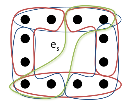
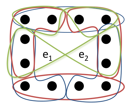
Figure 2 shows an example of a reducible balanced edge set $\mathcal{E}$. The separator is proper and consists of the single green edge $e_{s}$; it appears twice in the balanced edge set $\mathcal{E}$, once as a blue edge and once as a red edge. Figure 2 shows a reducible balanced edge set where the separator, consisting of the two green edges $e_{1}$ and $e_{2}$, is not proper. As before, the separator edges appear twice in the balanced edge set.

If $H$ is a hypergraph and $\mathcal{E}$ is a balanced edge set with $\supp(\mathcal{E})\subseteq H$, given a multiset $S$ with $\supp(S)\subseteq H$, we can construct a new balanced edge set in the following manner:

The previous example illustrates the algebraic interpretation of a splitting set. Notice there is a correspondence between monomials in $k[t_{e_{i}}]$ and multisets of edges of $H$. We will write $E(t_{e_{i_{1}}}^{a_{1}}t_{e_{i_{2}}}^{a_{2}}\cdots t_{e_{i_{l}}}^{a_{l}})$ for the multiset $(\{e_{i_{1}},\ldots,e_{i_{l}}\},f)$ where

Thus the support of $E(t_{e_{i_{1}}}^{a_{1}}t_{e_{i_{2}}}^{a_{2}}\cdots t_{e_{i_{l}}}^{a_{l}})$ corresponds to the support of the monomial $t_{e_{i_{1}}}^{a_{1}}t_{e_{i_{2}}}^{a_{2}}\cdots t_{e_{i_{l}}}^{a_{l}}$.

If $f_{\mathcal{E}}=u-v\in I_{H}$ is the binomial arising from the balanced edge set $\mathcal{E}$, then a monomial $s$ corresponds to a splitting set $S$ if and only if there exist two binomials $u_{1}-v_{1},u_{2}-v_{2}\in I_{H}$ such that $us=u_{1}u_{2}$, $vs=v_{1}v_{2}$ and $s=\gcd(v_{2},u_{1})$. In this case, the decomposition of $\mathcal{E}+S$ is $(\Gamma_{1},S,\Gamma_{2})$ where $\Gamma_{1}=E(u_{1})\sqcup_{m}E(v_{1})$ and $\Gamma_{2}=E(u_{2})\sqcup_{m}E(v_{2})$.

For a balanced edge set, $\mathcal{E}$, the existence of a spitting set determines whether the binomial $f_{E}\in I_{H}$ can be written as the linear combination of two binomials $f_{\Gamma_{1}}$,$f_{\Gamma_{2}}$ $\in I_{H}$. While, in general, the existence of a splitting set does not imply $\deg(f_{\Gamma_{1}}),\deg(f_{\Gamma_{2}})<\deg(f_{\mathcal{E}})$, if $H$ is uniform and the splitting set is proper, then the following lemma holds.

A binomial $f$ in a toric ideal $I$ is indispensable if $f$ or $-f$ belongs to every binomial generating set of $I$. Indispensable binomials of toric ideals were introduced by Takemura et al, and are studied in [1], [2], [3], [13], [15].

If every Graver basis element of a binomial ideal $I_{H}$ is indispensable, then the Graver basis of $I_{H}$ is the unique minimal generating set of $I_{H}$. Propositions 4.2 and 4.6 describe two classes of hypergraphs where this is the case. In particular, for these hypergraphs, the universal Gröbner basis of $I_{H}$ is a minimal generating set.

For the proof of Proposition 4.2, we make use of Proposition 3.2 in [14] which concerns balanced edge sets that are pairs of perfect matchings.

From the above discussion, we can see that if a uniform hypergraph $H$ contains an induced subhypergraph $H_{s}$ that is 2-regular and there exists a bicoloring such that with this bicoloring $H_{s}$ is also a balanced edge set, then the maximum degree of any minimal generating set of $I_{H}$ is at least $|E(H_{s})|/2$.

A similar statement holds for $k$-uniform, $k$-partite hypergraphs with vertex partition $V=\cup_{i=1}^{k}V_{i}$. Namely, if $H$ contains an induced subhypergraph $H_{s}$ that is 2-regular on $V_{i}$ (i.e., $H$ satisfies the conditions of Proposition 4.6) and there exists a bicoloring such that with this bicoloring $H_{s}$ is a balanced edge set (e.g., $H_{s}$ is a pair of disjoint perfect matchings), then the maximum degree of any minimal generating set of $I_{H}$ is at least $|E(H_{s})|/2$.

Recall that degree bounds on minimal generators give a Markov complexity bound for the corresponding log-linear model in algebraic statistics. This allows us to recover a well-known result:

For uniform hypergraphs, balanced edge sets are referred to as monomial walks. In the previous sections, we saw that splitting sets of $\mathcal{W}$ translate to algebraic operations on the binomials $f_{\mathcal{W}}$, providing a general construction for rewriting a high-degree binomial in terms of binomials corresponding to shorter walks. This, along with Lemma 3.5, is the key to the general degree bound result.

References

- [1] A. Takemura and S. Aoki. Some characterizations of minimal Markov basis for sampling from discrete conditional distributions, Ann. Inst. Statist. Math. 56 1 (2004), 1Ð17.
- [2] S. Aoki, A. Takemura, R. Yoshida. Indispensable monomials of toric ideals and Markov bases, Journal of Symbolic Computation 43 6Ð7 (2008) 490-507.
- [3] H. Charalambous, A. Katsabekis, and A. Thoma. Minimal systems of binomial generators and the indispensable complex of a toric ideal, Proceedings of the American Mathematical Society 135 (2007) 3443-3451.
- [4] J. De Loera and S. Onn, Markov bases of three-way tables are arbitrarily complicated, J. Symb. Comput. 41 2 (February 2006) 173-18.
- [5] M. Develin and S. Sullivant. Markov bases of binary graph models, Annals of Combinatorics 7 (2003) 441-466.
- [6] P. Diaconis and B. Sturmfels. Algebraic algorithms for sampling from conditional distributions, Ann. Statist. 26, no. 1, 363–397 (1998)
- [7] A. Dobra and S. Sullivant. A divide-and-conquer algorithm for generating Markov bases of multi-way tables. Computational Statistics 19 (2004), 347-366
- [8] M. Drton, B. Sturmfels and S. Sullivant. Lectures on algebraic statistics, Oberwolfach Seminars 39, Birkhäuser (2009)
- [9] I. Gitler, E. Reyes, R. Villarreal. Ring graphs and toric ideals, Electronic Notes in Discrete Mathematics 28 1 (2007) 393-400.
- [10] S. Hoşten and S. Sullivant. A finiteness theorem for Markov bases of hierarchical models, J. Comb. Theory Ser. A 114 2 (2007) 311-321.
- [11] L. Oeding. Set-theoretic defining equations of the tangential variety of the Segre variety, J. Pure and Applied Algebra, 215 (2011) 1516-1527.
- [12] H. Ohsugi and T. Hibi. Toric ideals generated by quadratic binomials, Journal of Algebra 218 (1999), 509-527.
- [13] H. Ohsugi and T. Hibi. Indispensable binomials of finite graphs, J. Algebra Appl. 4 (2005), no 4, 421-434.
- [14] S. Petrović and D. Stasi. Toric algebra of hypergraphs. Preprint: arXiv:1206.1904
- [15] E. Reyes, C. Tatakis, A. Thoma. Minimal generators of toric ideals of graphs, Adv. in Appl. Math 48 (2012), no. 1, 64-67
- [16] B. Sturmfels. Gröbner bases and convex polytopes, University Lecture Series, 8. American Mathematical Society, 1996.
- [17] B. Sturmfels and S. Sullivant. Toric ideals of phylogenetic invariants, Journal of Computational Biology 12 (2005) 204-228.
- [18] B. Stumfels and P. Zwiernik. Binary cumulant varieties, Annals of Combinatorics, to appear.
- [19] C. Tatakis andA. Thoma. On the universal Gröbner basis of toric ideals of graphs, Journal of Combinatorial Theory, Series A, 118 (2011) 1540-1548
- [20] R. Villarreal. Rees algebras of edge ideals, Communications in Algebra, 23 (9), 3513–3524 (1995)
- [21] R. Villarreal, Monomial Algebras. Monographs and Textbooks in Pure and Applied Mathematics 238, Marcel Dekker, Inc., New York, 2001.