Improved Inapproximability for TSP

As mentioned, we will view TSP as the problem of selecting edges from $E$ to form a minimum-weight multi-set $E_{T}$ that makes the graph Eulerian. It is easy to see that no edge will be selected more than twice, since if an edge is selected three times we can remove two copies of it from $E_{T}$ and the graph will still be Eulerian while we have improved the cost.

In our construction we would like to be able to stipulate that some edges are to be used at least once in any valid tour. We can achieve this with the following trick: suppose that there is an edge $(u,v)$ with weight $w$ that we want to force into every tour. We sub-divide this edge a large number of times, say $p-1$, that is, we remove the edge and replace it with a path of $p$ edges going through new vertices of degree two. We then redistribute the original edge’s weight to the $p$ newly formed edges, so that each has weight $w/p$. Now, any tour that fails to use two or more of the newly formed edges must be disconnected. Any tour that fails to use exactly one of them can be augmented by adding two copies of the unused edge. This only increases the cost by $2w/p$, which can be made arbitrarily small by giving $p$ an appropriately large value. Therefore, we may assume without loss of generality that in our construction we can force some edges to be used at least once. Note that these arguments apply also to quasi-tours.

In $I_{1}$ each variable appears at most a constant number of times $B$, where $B$ depends on $\epsilon$. We would like to reduce the maximum number of occurrences of each variable to a small absolute constant. For this, one typically uses some kind of expander or amplifier construction. Here we will rely on a construction due to Berman and Karpinski that reduces the number of occurrences to 5.

We now use the above construction to construct a system of equations where each variable appears exactly 5 times. First, we may assume that in $I_{1}$ the number of appearances of each variable is a multiple of 5 (otherwise, repeat all equations five times). Also, by repeating all the equations we can make sure that all variables appear at least $B^{\prime}$ times, where $B^{\prime}$ is a sufficiently large number to make Theorem 3.2 hold.

For each variable $x_{i}$ in $I_{1}$ we introduce the variables $x_{(i,j)},j\in[d(i)]$ and $y_{(i,j)},j\in[0.8d(i)]$ where $d(i)$ is the number of appearances of $x_{i}$ in the original instance. We call $X_{i}=\{x_{(i,j)}\ |\ j\in[d(i)]\}\cup\{y_{(i,j)}\ |\ j\in[0.8d(i)]\}$ the cloud that corresponds to $x_{i}$. Construct a bipartite graph with the property described in Theorem 3.2 with $L=[d(i)],R=[0.8d(i)]$ (since $d(i)<B$ is a constant that depends only on $\epsilon$ this can be done in constant time by brute force). For each edge $(j,k)\in E$ introduce the equation $x_{(i,j)}+y_{(i,k)}=1$. Finally, for each equation $x_{i_{1}}+x_{i_{2}}+x_{i_{3}}=b$ in $I_{1}$, where this is the $j_{1}$-th appearance of $x_{i_{1}}$, the $j_{2}$-th appearance of $x_{i_{2}}$ and the $j_{3}$-th appearance of $x_{i_{3}}$ replace it with the equation $x_{(i_{1},j_{1})}+x_{(i_{2},j_{2})}+x_{(i_{3},j_{3})}=b$.

Denote this instance by $I_{2}$ and we have $|I_{2}|=13m$, with $12m$ equations having size 2. A consistent assignment to a cloud $X_{i}$ is an assignment that sets all $x_{(i,j)}$ to $b$ and all $y_{(i,j)}$ to $1-b$. By standard arguments using the graph of Theorem 3.2 we can show that an optimal assignment to $I_{2}$ is consistent (in each inconsistent cloud let $S$ be the vertices with the minority assignment; flipping all variables of $S$ cannot make the solution worse). From this it follows that it is NP-hard to distinguish if the maximum number of satisfiable equations is at least $(13-\epsilon)m$ or at most $(12.5+\epsilon)m$.

In the MAX-1-in-3-SAT problem we are given a collection of clauses $(l_{i}\lor l_{j}\lor l_{k})$, each consisting of at most three literals, where each literal is either a variable or its negation. A clause is satisfied by a truth assighment if exactly one of its literals is set to True. The problem is to find an assignment that satisfies the maximum number of clauses.

We would like to produce a MAX-1-in-3-SAT instance from $I_{2}$. Observe that it is easy to turn the size two equations $x_{(i,j)}+y_{(i,k)}=1$ to the equivalent clauses $(x_{(i,j)}\lor y_{(i,k)})$. We only need to worry about the $m$ equations of size three.

If the $k$-th size-three equation of $I_{2}$ is $x_{(i_{1},j_{1})}+x_{(i_{2},j_{2})}+x_{(i_{3},j_{3})}=1$ we introduce three new auxilliary variables $a_{(k,i)},i\in[3]$ and replace the equation with the three clauses $(x_{(i_{1},j_{1})}\lor a_{(k,1)}\lor a_{(k,2)})$, $(x_{(i_{2},j_{2})}\lor a_{(k,2)}\lor a_{(k,3)})$, $(x_{(i_{3},j_{3})}\lor a_{(k,1)}\lor a_{(k,3)})$. If the right-hand-side of the equation is $0$ then we add the same three clauses except we negate $x_{(i_{1},j_{1})}$ in the first clause. We call these three clauses the cluster that corresponds to the $k$-th equation.

It is not hard to see that if we fix an assignment to $x_{(i_{1},j_{1})},x_{(i_{2},j_{2})},x_{(i_{3},j_{3})}$ that satisfies the $k$-th equation of $I_{2}$ then there exists an assignment to $a_{(k,1)},a_{(k,2)},a_{(k,3)}$ that satisfies the whole cluster. Otherwise, at most two of the clauses of the cluster can be satisfied. Furthermore, in this case there exist three different assignments to the auxilliary variables that satisfy two clauses and each leaves a different clause unsatisfied.

From now on, we will denote by $M$ the set of (main) variables $x_{(i,j)}$, by $C$ the set of (checker) variables $y_{(i,j)}$ and by $A$ the set of (auxilliary) variables $a_{(k,i)}$. Call the instance of MAX-1-in-3-SAT we have constructed $I_{3}$. Note that it consists of $15m$ clauses and $8.4m$ variables.

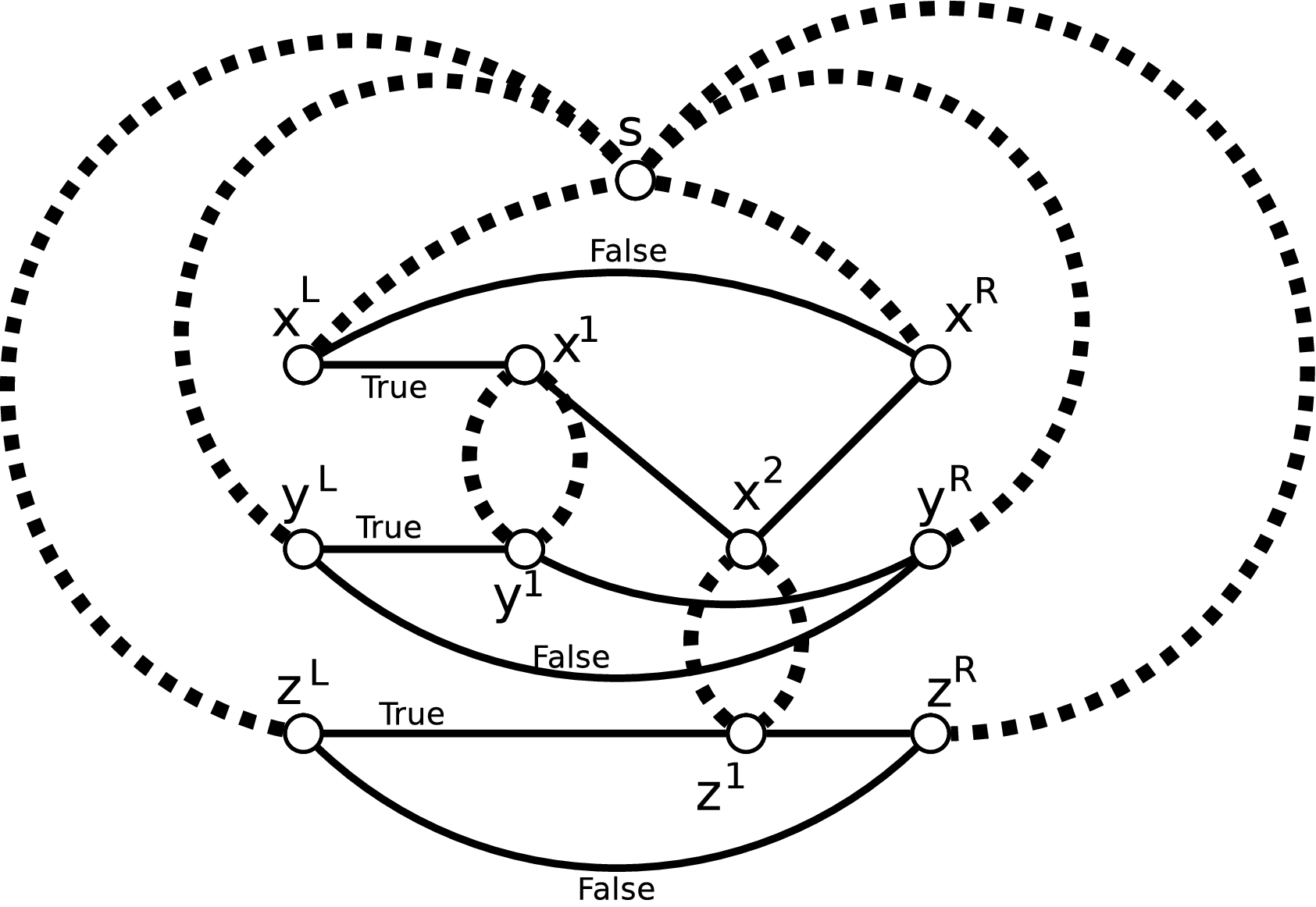
We now describe a construction that encodes $I_{3}$ into a TSP instance $G(V,E)$. Rather than viewing this as a generic construction from MAX-1-in-3-SAT to TSP, we will at times need to use facts that stem from the special structure of $I_{3}$. In particular, the fact that variables can be partitioned into sets $M,C,A$, such that variables in $M\cup C$ appear five times and variables in $A$ appear twice; the fact that most clauses have size two and they involve one positive variable from $M$ and one positive variable from $C$; and also the fact that clauses of size three come in clusters as described in the construction of $I_{3}$.

As mentioned, we assume that in the graph $G(V,E)$ we may include some forced edges, that is, edges that have to be used at least once in any tour. The graph includes a central vertex, which we will call $s$. For each variable in $x\in M\cup C\cup A$ we introduce two new vertices named $x^{L}$ and $x^{R}$, which we will call the left and right terminal associated with $x$. We add a forced edge from each terminal to $s$. For terminals that correspond to variables in $M\cup C$ this edge has weight $7/4$, while for variables in $A$ it has weight $1/2$. We also add two (parallel) non-forced edges between each pair of terminals representing the same variable, each having a weight of 1 (we will later break down at least one from each pair of these, so the graph we will obtain in the end will be simple). Informally, these two edges encode an assignment to each variable: we arbitrarily label one the True edge and the other the False edge, the idea being that a tour should pick exactly one of these for each variable and that will give us an assignment. We will re-route these edges through the clause gadgets as we introduce them, depending on whether each variable appears in a clause positive or negative.

Now, we add some gadgets to encode the size-two clauses of $I_{3}$. Let $(x_{(i,j_{1})}\lor y_{(i,j_{2})})$ be a clause of $I_{3}$ and suppose that this is the $k_{1}$-th clause that contains $x_{(i,j_{1})}$ and the $k_{2}$-th clause that contains $y_{(i,j_{2})}$, $k_{1},k_{2}\in[5]$. Then we add two new vertices to the graph, call them $x_{(i,j_{1})}^{k_{1}}$ and $y_{(i,j_{2})}^{k_{2}}$. Add two forced edges between them, each of weight $3/2$ (recall that forced edges represent long paths, so these are not really parallel edges). Finally, re-route the True edges incident on $x_{(i,j_{1})}^{L}$ and $y_{(i,j_{2})}^{L}$ through $x_{(i,j_{1})}^{k_{1}}$ and $y_{(i,j_{2})}^{k_{2}}$ respectively. More precisely, if the True edge incident on $x_{(i,j_{1})}^{L}$ connects it to some other vertex $u$, remove that edge from the graph and add an edge from $x_{(i,j_{1})}^{L}$ to $x_{(i,j_{1})}^{k_{1}}$ and an edge from $x_{(i,j_{1})}^{k_{1}}$ to $u$. All these edges have weight one and are non-forced (see Figure 1).

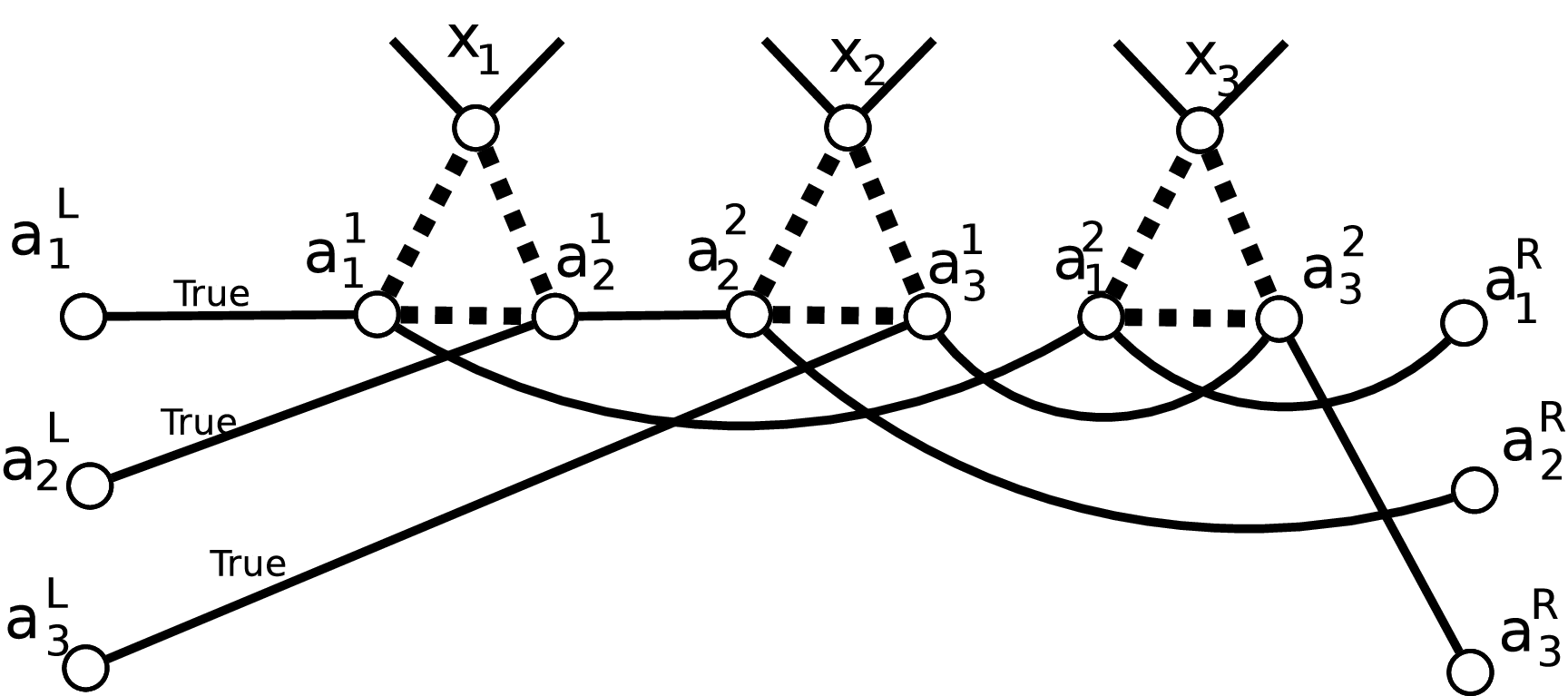
We use a similar gadget for clauses of size three. Consider a cluster $(x_{(i_{1},j_{1})}\lor a_{(k,1)}\lor a_{(k,2)})$, $(x_{(i_{2},j_{2})}\lor a_{(k,2)}\lor a_{(k,3)})$, $(x_{(i_{3},j_{3})}\lor a_{(k,1)}\lor a_{(k,3)})$ and suppose for simplicity that this is the fifth appearance for all the main variables of the cluster. Then we add the new vertices $x_{(i_{1},j_{1})}^{5},x_{(i_{2},j_{2})}^{5},x_{(i_{3},j_{3})}^{5}$ and also the vertices $a_{(k,1)}^{1},a_{(k,1)}^{2},a_{(k,2)}^{1},a_{(k,2)}^{2}$ and $a_{(k,3)}^{1},a_{(k,3)}^{2}$. To encode the first clause we add two forced edges of weight $5/4$, one from $x_{(i_{1},j_{1})}^{5}$ to $a_{(k,1)}^{1}$ and one from $x_{(i_{1},j_{1})}^{5}$ to $a_{(k,2)}^{1}$. We also add a forced edge of weight 1 from $a_{(k,1)}^{1}$ to $a_{(k,2)}^{1}$, thus making a triangle with the forced edges (see Figure 2). We re-route the True edge from $a_{(k,1)}^{L}$ through $a_{(k,1)}^{1}$ and $a_{(k,1)}^{2}$. We do similarly for the other two auxilliary variables and the main variables. Finally, for a cluster where $x_{(i_{1},j_{1})}$ is negated, we use the same construction except that rather than re-routing the True edge that is incident on $x_{(i_{1},j_{1})}^{L}$ we re-route the False edge. This completes the construction.

Let us now prove one direction of the reduction and in the process also give some intuition about the construction. Call the graph we have constructed $G(V,E)$.

We would like now to prove the converse of Lemma 1, namely that if a tour of cost $L+k$ exists then we can find an assignment that leaves at most $k$ clauses unsatisfied. Let us first give some high-level intuition and in the process justify the weights we have selected in our construction.

Informally, we could start from a simple base case: suppose that we have a tour such that all edges of $G$ are used at most once. It is not hard to see that this then corresponds to an assignment, as in the proof of Lemma 1. So, the problem is how to avoid tours that may use some edges twice.

To this end, we first give some local improvement arguments that make sure that the number of problematic edges, which are used twice, is limited. However, arguments like these can only take us so far, and we would like to avoid having too much case analysis.

We therefore try to isolate the problem. For variables in $M\cup C$ which the tour treats honestly, that is, variables which are not involved with edges used twice, we directly obtain an assignment from the tour. For the other variables in $M\cup C$ we pick a random value and then extend the whole assignment to $A$ in an optimal way. We want to show that the expected number of unsatisfied clauses is at most $k$.

The first point here is that if a clause containing only honest variables turns out to be violated, the tour must also be paying an extra cost for it. The difficulty is therefore concentrated on clauses with dishonest variables.

By using some edges twice the tour is paying some cost on top of what is accounted for in $L$. We would like to show that this extra cost is larger than the number of clauses violated by the assignment. It is helpful to think here that it is sufficient to show that the tour pays an additional cost of $\frac{5}{2}$ for each dishonest variable, since main variables appear 5 times.

A crucial point now is that, by a simple parity argument, there has to be an even number of violations (that is, edges used twice) for each variable (Lemma 4). This explains the weights we have picked for the forced edges in size-three gadgets ($\frac{5}{4}$) and for edges connecting terminals to $s$ ($\frac{7}{4}=\frac{5}{4}+\frac{1}{2}$ or $\frac{5}{4}$ extra to the cost already included in $L$ for fixing the parity of the terminal vertex). Two such violations give enough extra cost to pay for the expected number of unsatisfied clauses containing the variable.

At this point, we could also set the weights of forced edges in size-two gadgets to $\frac{5}{2}$, which would be split among the two dishonest variables giving $\frac{5}{4}$ to each. Then, any two violations would have enough additional cost to pay for the expected unsatisfied clauses. However, we are slightly more careful here: rather than setting all dishonest variables in $M\cup C$ independently at random, we pick a random but consistent assignment for each cloud. This ensures that all size-two clauses with violations will be satisfied. Thus, it is sufficient for violations in them to have a cost of $\frac{3}{2}$: the amount "paid" to each variable is now $\frac{3}{4}=\frac{5}{4}-\frac{1}{2}$, but the expected number of unsatisfied clauses with this variable is also decreased by $\frac{1}{2}$ since one clause is surely satisfied.

Let us now proceed to give the full details of the proof. Recall that if a tour of a certain cost exists, then there exists also a quasi-tour of the same cost. It suffices then to prove the following:

In order to prove Lemma 2 it is helpful to first make some easy observations. First, observe that if a quasi-tour uses a unit-weight edge twice then we can remove both of these appearances of the edge from the solution without increasing the cost, since the number of components can only increase by one. Therefore, all (non-forced) edges of weight one are used at most once.

Second, if both forced edges of a gadget of size two are used twice then we can remove one appearance of each from the solution, decreasing the cost. Similarly, in a gadget of size three if two forced edges are used twice then we can drop one copy of each and use the third edge twice, making the tour cheaper. Therefore, in each gadget there is at most one forced edge that is used twice.

Third, if both forced edges that connect the terminals $x^{L},x^{R}$ to $s$ are used twice, then we can remove one appearance of each from the solution and replace them by the shortest path from $x^{L}$ to $x^{R}$ that uses only non-forced unit weight edges. This has weight at most one for the auxilliary variables and two for the rest, which in both cases is at most as much as the weight of the removed edges. Therefore, for each variable $x$, at least one of the forced edges that connect $x^{L},x^{R}$ to $s$ is used exactly once.

Given a tour $E_{T}$, we will say that a variable $x$ is honestly traversed in that tour if all the forced edges that involve it are used exactly once (this includes the forced edges incident on $x^{L},x^{R}$ and $x^{i}$, $i\in[5]$).

Let us now give two more useful facts.

Observe that it follows from Lemmata 3,4 that if all the main variables involved in a cluster are honest then the auxilliary variables of that cluster are also honest. This holds because if the main variables are honest then by Lemma 3 no forced edge inside the gadgets of the cluster is used twice, so by Lemma 4 and the fact that at least one of the forced edges incident on the terminals is used once, the auxilliary variables are honest.

We would like now to be able to extract a good assignment even if a tour is not honest, thus indirectly proving that honest tours are optimal.

References

- [1] P. Berman and M. Karpinski. On some tighter inapproximability results (extended abstract). In J. Wiedermann, P. van Emde Boas, and M. Nielsen, editors, ICALP, volume 1644 of Lecture Notes in Computer Science, pages 200–209. Springer, 1999.
- [2] P. Berman and M. Karpinski. Efficient amplifiers and bounded degree optimization. Electronic Colloquium on Computational Complexity (ECCC), 8(53), 2001.
- [3] P. Berman and M. Karpinski. Improved approximation lower bounds on small occurrence optimization. Electronic Colloquium on Computational Complexity (ECCC), 10(008), 2003.
- [4] H.-J. Böckenhauer, J. Hromkovic, R. Klasing, S. Seibert, and W. Unger. An improved lower bound on the approximability of metric tsp and approximation algorithms for the tsp with sharpened triangle inequality. In H. Reichel and S. Tison, editors, STACS, volume 1770 of Lecture Notes in Computer Science, pages 382–394. Springer, 2000.
- [5] L. Engebretsen. An explicit lower bound for tsp with distances one and two. Algorithmica, 35(4):301–318, 2003.
- [6] S. O. Gharan, A. Saberi, and M. Singh. A randomized rounding approach to the traveling salesman problem. In Ostrovsky [11], pages 550–559.
- [7] J. Håstad. Some optimal inapproximability results. Journal of the ACM (JACM), 48(4):798–859, 2001.
- [8] M. Karpinski and R. Schmied. On approximation lower bounds for tsp with bounded metrics. CoRR, abs/1201.5821, 2012.
- [9] T. Mömke and O. Svensson. Approximating graphic tsp by matchings. In Ostrovsky [11], pages 560–569.
- [10] M. Mucha. 13/9-approximation for graphic tsp. In C. Dürr and T. Wilke, editors, STACS, volume 14 of LIPIcs, pages 30–41. Schloss Dagstuhl - Leibniz-Zentrum fuer Informatik, 2012.
- [11] R. Ostrovsky, editor. IEEE 52nd Annual Symposium on Foundations of Computer Science, FOCS 2011, Palm Springs, CA, USA, October 22-25, 2011. IEEE, 2011.
- [12] C. H. Papadimitriou and S. Vempala. On the approximability of the traveling salesman problem (extended abstract). In F. F. Yao and E. M. Luks, editors, STOC, pages 126–133. ACM, 2000.
- [13] C. H. Papadimitriou and S. Vempala. On the approximability of the traveling salesman problem. Combinatorica, 26(1):101–120, 2006.
- [14] C. H. Papadimitriou and M. Yannakakis. The traveling salesman problem with distances one and two. Mathematics of Operations Research, pages 1–11, 1993.
- [15] A. Sebö and J. Vygen. Shorter tours by nicer ears:. CoRR, abs/1201.1870, 2012.