Incorporating Ambipolar and Ohmic Diffusion in the AMR MHD code RAMSES
Abstract
We have implemented non-ideal Magneto-Hydrodynamics (MHD) effects in the Adaptive Mesh Refinement (AMR) code RAMSES, namely ambipolar diffusion and Ohmic dissipation, as additional source terms in the ideal MHD equations. We describe in details how we have discretized these terms using the adaptive Cartesian mesh, and how the time step is diminished with respect to the ideal case, in order to perform a stable time integration. We have performed a large suite of test runs, featuring the Barenblatt diffusion test, the Ohmic diffusion test, the C-shock test and the Alfven wave test. For the latter, we have performed a careful truncation error analysis to estimate the magnitude of the numerical diffusion induced by our Godunov scheme, allowing us to estimate the spatial resolution that is required to address non-ideal MHD effects reliably. We show that our scheme is second-order accurate, and is therefore ideally suited to study non-ideal MHD effects in the context of star formation and molecular cloud dynamics.
Keywords:
stars: formation — ISM: magnetic fields — methods: numericalI Introduction
The impact of magnetic fields on various objects in astrophysics is now well established. They play a major role on a wide range of scales, from the study of the early universe, the stellar and intergalactic medium to the formation and interiors of stars or the accretion flows around stellar objects. They are difficult to study both from an observational and a theoretical (and numerical) point of view. Several implementations of ideal MHD have been performed since the last decade (Fromang et al. [12], Stone & Norman [33], Machida et al. [25] among others), and numerical issues concerning the divergence free condition have now been resolved. However, ideal magnetohydrodynamics (MHD) is in many circumstances a poor approximation and non-ideal MHD effects need to be thoroughly considered.
Ambipolar diffusion is expected to play a major role in star formation (Mestel & Spitzer [27]), at the scale of molecular clouds by enabling the collapse of otherwise magnetically supported clouds (Basu & Ciolek [4]) and at the scale of the first Larson’s core with the formation of a centrifugally supported disk and the well-known fragmentation crisis (Hennebelle & Teyssier [14]). Ambipolar diffusion is also important in protoplanetary disks as they are in general only partially ionised. The microscopic and entropic heating resulting from the drift and collision between neutral and charged species is another very important and relatively unknown aspect which is crucial as soon as cooling or heating of the gas (thus radiative transfert) is taken into account (in contrast it is not relevant when using a barotropic equation of state).
Magnetic resistivity effects range from prohibiting long-term MHD turbulence in molecular clouds (Basu & Dapp [5]) to preventing the magnetic braking catastrophe on small scales (Dapp & Basu [8]). Its importance is also crucial in order to study disk formation around protostellar objects (Krasnopolsky et al. [16]) and the physics of binary formation and brown dwarfs.
Thus, it appears necessary to introduce the ambipolar and Ohmic diffusion in a 3D MHD code. Before exploring the astrophysical impact of such a study, however, the accuracy of the treatment of the complete MHD set of equations must be unambiguously assessed. This is the very aim of the present paper, in which we describe a prescription to incorporate ambipolar and Ohmic diffusion in the multi-dimensional MHD AMR code RAMSES (Teyssier [34]), extending the ideal MHD version presented in Teyssier et al. [35] and Fromang et al. [12].
Several numerical treatments have been derived from ideal MHD models, following different aims and thus using different methods. The first attempt to implement ambipolar diffusion in a code was made by Black & Scott [6] using an iterative approximation in an implicit first-order code. Toth [38] used a semi-explicit method in a two-dimensional code to investigate instabilities in C-schocks. Mac Low et al. [20] presented a widely used explicit method (Choi et al. [7], Mellon & Li [26], Li et al. [19]) to implement single-fluid ambipolar diffusion in the strong coupling limit, and then developed a two-fluid model in order to capture shock instabilities. Tilley & Balsara [36] and more recently Tilley & Balsara [37] presented a semi-implicit scheme for solving two-fluid ambipolar diffusion, arguing that the single fluid approximation does not carry the full set of MHD waves that can propagate in a poorly ionized system. Multi-fluid approaches including ambipolar diffusion and Ohmic diffusion have been suggested by [11], or [29] and then investigated by e.g. Kunz & Mouschovias [17]. Recently, Li et al. [19] used the single-fluid approach including more realistic resistivities based on a multi-fluid approach for ambipolar diffusion, Ohmic diffusion and Hall effect in two-dimensional (axi-symmetric) calculations. Another approach has been used by Machida et al. [21] was to describe both ambipolar diffusion and Ohmic diffusion in one single Laplace operator , with taking into account every diffusive process at stake. These numerous studies have also given rise to several numerical tests, a number of which we will either perform directly or slightly modify to assess the accuracy of our treatment.
Our current study focusses on the one-fluid approximation (Shu et al. [32]), as in previous calculations by Mac Low et al. [20] and Duffin & Pudritz [9]. We used a direct explicit method to implement non-ideal MHD terms in both the induction and energy equations (Mac Low et al. [20]) in an AMR framework. We did not choose to account for non-ideal effects by adding ambipolar diffusion and Ohmic dissipation in a single Laplace operator as Machida et al. [21]. Instead we kept the full expressions and proceeded separately for each non-ideal effect.
The paper is organized as follows. In § II, we first derive the equations for ambipolar diffusion in the single fluid approximation. We then describe the various tests we have performed, first without the hydrodynamics and then in a complete MHD situation, exploring in particular the propagation of Alfvén waves. Comparisons with existing analytical or benchmark solutions are presented in details, demonstrating the validity and the accuracy of our scheme. § III addresses the case of Ohmic diffusion, following the same procedure as for ambipolar diffusion, while § IV is devoted to the conclusion.
II Ambipolar diffusion
II.1 Equations
When the ions pressure and momentum are negligible compared to those of neutral species (as is the case for example in molecular clouds), the Lorentz force exerted on the ions is in equilibrium with the drag force exerted by the neutrals, which corresponds to a situation of strong coupling between the neutral fluid and the field lines. In such a situation, the plasma can be adequately described by a single fluid (Shu et al. [32] and Choi et al. [7]) of mass density , and neutrals and ions mass densities and respectively. Interestingly, in the case of the one-fluid approximation the results can be directly compared with the ones obtained with ideal MHD giving clear insights about MHD wave propagation properties in the non-ideal case (Balsara [2]).The present study is devoted to the technical resolution of the resistive MHD equations and we will also ignore gravity (and thus the Poisson equation). The MHD equations are given by the usual continuity, momentum, energy and induction equations, completed by the magnetic field divergence-free condition (in rational units, ):
| (1) | ||||
| (2) | ||||
| (3) | ||||
| (4) | ||||
| (5) |
denotes the total energy
| (6) |
where is the specific internal energy.
is the total pressure
| (7) |
where is the adiabatic index.
denotes the Lorentz force
| (8) |
with
| (9) |
The ambipolar electromagnetic force (EMF) is given by
| (10) |
where and denote respectively the ions and neutrals velocities, and is the drift coefficient between ions and neutrals due to ambipolar diffusion. The last equality in Equation (10) illustrates the balance between magnetic and drag forces in the ion fluid, while Equation (3) is accounting for ambipolar heating of neutrals by ions (Shu [31]). In order to write both Equation (3) and Equation (10) we need to assume that the velocity drift between ions and neutrals and the one between electrons and neutrals are not too different (by a factor ). Therefore, as long as the Hall effect is negligible, these equations remain valid (see Pinto et al. [30] for a more detailed study).
Equation (3) (the conservation of energy: ) is equivalent to
| (11) |
where we can see that the neutrals-ions friction term heats up the gas and increases the entropy.
II.2 Computing the ambipolar diffusion terms
In this section, we describe the numerical implementation of the previous equations, focusing on the ambipolar diffusion terms in the energy and induction equations.
II.2.1 The ambipolar EMF
The ambipolar term in the induction equation can be considered as an additional electromotive force (EMF). To update the magnetic field the values of the EMF have to be defined as time and space averages along cell edges (Teyssier et al. [35]). For instance, the EMF in the direction is defined at (and the same for the other directions with circular permutations) where i,j and k are the cell indices in the directions respectively.
We focus now on the EMF in the direction, defined at and explain in details how it is computed. writes
| (12) |
with the drift velocity . We therefore have to evaluate and at , and then calculate
| (13) |
The RAMSES code is based on the Constrained Transport scheme for the magnetic field evolution (Teyssier et al. [35]), for which the components of the magnetic field are defined at the center of cell faces: if are the coordinates of a cell center, is defined at position , at and at (see Figure 1). Each magnetic field component is computed using the finite-surface approximation, which reads for the x component:
| (14) |
while other components are defined by circular permutations.
We also need to define the drift velocity at using the Lorentz force , the density and the ions density . The two latter quantities are cell-centered quantities (in contrast to the magnetic field):
| (15) |
and
| (16) |
We then define the edge-centered density (and the ions edge-centered density) as an arithmetic average of surrounding cells (see Figure 1, right panel):
| (17) |


This definition is adapted for the components of the magnetic field to compute them at (see Figure 2):
| (18) | ||||
| (19) |


Given the Lorentz force at (see Sections II.2.2 and II.2.3), it is possible to compute the first component (z direction, with unit vector ) of the ambipolar EMF: , while the two other components are obtained through circular permutations.
These ambipolar EMFs are then added to the ideal MHD EMFs calculated with a 2D Riemann solver, as described in Teyssier et al. [35] and Fromang et al. [12].
II.2.2 The Lorentz force as the product of the current and the magnetic field
We now focus on the computation of the Lorentz force at . The first way to calculate this term is to explicitly compute the magnetic field components and the current at , as:
| (20) |
is naturally defined at and and are naturally defined respectively at and . In order to have all three components of at the location of the EMF () we need to use the magnetic field components at specific positions, as follows:
| (21) | ||||
| (22) | ||||
| (23) |
As above, we have to express each of these terms through arithmetic averages of the naturally defined components of the magnetic field:
| and | (24) | ||||
| and | (25) | ||||
| and | (26) |
and are naturally defined at and respectively, and thus the two terms in Equation (24) need not to be computed again.
The terms in Equation (25) and Equation (26) are obtained thanks to averages on four components (see Figure 3):
| (27) | ||||
| (28) | ||||
| (29) | ||||
| (30) |


The Lorentz force for the other components of the EMF ( and directions) are obtained through circular permutations.
II.2.3 The Lorentz force as the divergence of a flux
Another way to compute the Lorentz force is to express it as the divergence of a well chosen flux:
| (31) |
and
| (32) |
with and .
Let us focus on the component of the Lorentz force for the EMF in the direction. It reads:
| (33) |
In order to compute the Lorentz force at , we compute each term at specific positions:
| (34) | ||||
| (35) | ||||
| (36) |
We then only need to compute each component of the magnetic field at in order to get the EMF in the direction.
As explained in the previous paragraph, an average over well chosen (where the magnetic field is naturally defined) surrounding cells is used (see Figures 2 and 4):
| (37) | ||||
| (38) | ||||
| (39) | ||||
| (40) | ||||
| (41) |
and
| (42) | ||||
| (43) | ||||
| (44) |

Again and as highlighted previously, in order to get the two other components of the EMF one only needs to perform circular permutations.
These two methods (described in Sections II.2.2 and II.2.3) to compute the Lorentz force are implemented in RAMSES and show similar performances. This method might work better under certain conditions, for a particular setup of the magnetic field lines. Nonetheless, when counting the number of floating point operations, the computer performs using this method 4911 more additions and 8047 more multiplications for a given cell than with the previously described method.
II.2.4 Contribution of ambipolar diffusion to the energy flux
II.2.5 Computation of the time step in presence of ambipolar diffusion
The ambipolar diffusion timescale can be estimated through the drift velocity of ions. Recalling Equation (10) we get:
| (46) |
where is a characteristic length for ambipolar diffusion, which can be estimated as . We then have the timescale:
| (47) |
Written as a diffusion, with the ambipolar diffusion coefficient , where is the Alfvén speed and is the characteristic collision time between ions and neutrals. A Von Neumann analysis for the diffusion part of the equation can be performed for the scheme used:
| (48) |
It can be differenced (in one dimension):
| (49) |
Using ,
| (50) |
Equation (50) shows that the scheme is stable according to Von Neumann stability analysis provided the coefficient is lower than 0.5:
| (51) |
For the three dimensional case, this time-step constraint is more stringent than for the one dimensional case presented above.
Therefore, the time step used to update the solution is computed by taking the minimum of the usual MHD Courant condition (Fromang et al. [12]) and the ambipolar timestep defined by
| (52) |
where the minimum is taken over all the cells of the computational grid. The coefficient is taken to achieve better convergence. This choice is based on the various tests performed, and might not be suited to all other problems. As can be noted in equation (52), the time-step scales as . Even though this is very demanding in terms of numerical resources as the grid becomes more and more refined, there are means to speed-up the calculations, as explained in the following paragraph.
The ambipolar time step is proportional to (see Equation (52)), which is assumed to be proportional to : (see Elmegreen [10]). Both the factor () and the power law () are very dependent on the microphysics and the geometry of the grains. This assumption is thus made for the sake of simplicity, but might not always be valid. In some cases, for example in star formation simulations, the time-step can become unphysically small in very diffuse regions where the ionisation approximated as above (Equation (52)) is very small. Following Nakamura & Li [28], we use a threshold in order to limit the time-step when needed. On the other hand, in very dense parts where the grid is fairly refined (where is small), the dependence of and with the density prevent the time-step from becoming too becoming too small. This situation has to be studied for each different physical problem and can’t be assumed once and for all. We will address this issue in the case of star-formation in a forthcoming paper.
II.3 The AMR scheme
The AMR algorithm used in RAMSES is described in Teyssier [34], and its extension to MHD is first described in Teyssier et al. [35] and then in Fromang et al. [12]. We briefly recall the main features here. It is a tree-based AMR code whose data structure is a ’Fully Threaded Tree” (Khokhlov [15]). The grid is divided into ”octs” which are groups of 8 cells with the same parent cell. The first level of refinement () corresponds to the unit cube, which defines the computational domain. The grid is recursively refined from the to the minimum level of refinement , in order to build the base Cartesian grid. Adaptive refinement then proceeds from this coarse grid up to the user-defined maximum level of refinement . When the computational grid is a traditional Cartesian grid. Issues arise when refined cells are created, in the case where . Concerning the non-ideal MHD, the EMF and energy fluxes are simply added to the existing ideal MHD EMF and fluxes. As a consequence, there are no more complications in refining and derefining cells than in the ideal MHD case.
II.3.1 Divergence-free prolongation operator: refining cells
The ”prolongation operator” is the creation of a new ”oct” of 8 cells when a cell is newly refined. Cell-centered variables and magnetic field components are needed for each refined cell. This is usually done using a conservative interpolation of the variables, yet in the case of magnetic fields, the divergence-free constraint has to be fulfilled by each of the new cells which makes things more complicated in details. A critical step has been solved by Balsara [3] and Toth & Roe [39] in the constrained transport framework. The idea developed in those articles is to use slope limiters to interpolate the magnetic field components in each parent face conserving the flux, and then to perform a three dimensional (which is divergence-free inside the cell volume) reconstruction in order to compute the new magnetic field components for each children faces. The same slope limiters as the ones used in the Godunov scheme for the hydrodynamics are used in this step.
II.3.2 Magnetic flux corrections: derefining cells
The ”Restriction Operator” is, in the multigrid terminology, the operation of derefining a split cell. The divergence-free constraint still needs to be satisfied, so that the magnetic field components in the coarse faces are simply the arithmetic averages of the four fine faces values. This is the parallel in MHD of the ”flux correction step” for the Euler system.
II.3.3 EMF corrections
This is specific to the induction equation: for a coarse face adjacent to a refined face, the coarse EMF in the conservative update of the solution needs to be replaced by the arithmetic average of the two fine EMF vectors. This is mandatory to guarantee that the magnetic field remains divergence-free even at coarse/fine boundaries.
II.4 Tests for the ambipolar diffusion
II.4.1 The Barenblatt diffusion test
In this section, we first test the accuracy of the calculation of the ambipolar term alone. For sake of simplicity, we assume that the magnetic field has the form , with and , that all the velocities remain equal to zero and that density and thermal pressure are constant. The induction equation takes the form of a diffusion equation:
| (53) |
which can also be written in compact form:
| (54) |
This is a non-linear diffusion equation, since the diffusion coefficient, , depends non-linearly on the magnetic field. Here, denotes the y-component of the Alfvén velocity. The solution of this problem with a Dirac pulse as initial condition (known as the Barenblatt-Pattle solutions) has been derived by Grundy & McLaughlin [13] (See Appendix A for more details about the analytical solution).
The initial states in one and two dimensions are respectively:
with being the cell size at the lowest level of refinement used (in this case: 3). This ensures that the initial perturbation is the same for the case of an AMR grid and a fully refined grid.
We performed the test both with a uniform grid and using the AMR with the same maximum level. The level of refinement refers to the number of cells used: cells are used for the level of refinement in a -dimensional calculation. As seen in the figures, the agreement between the numerical and the analytical curves is excellent, a few tenths of a percent on average. The results obtained on an AMR grid (with levels varying from 3 to 7, corresponding to a mesh size and ) are almost as good as the ones obtained on a regular grid corresponding to the highest level of refinement (level 7, with a cell size and 128 cells): the maximum relative error is less than one percent except where the magnetic field equals zero. The difference between AMR and uniform grid is less than for values of magnetic field of about .
The grid is refined if the gradient of magnetic field is greater than 0.1 (this insures for this test that the error on the AMR grid and on the regular grid are about the same). We also checked that the same accuracy is obtained for any orientation of the magnetic field (using or instead of ). Figure 7 represents the evolution of the error calculated as as function of the mesh size ( being the number of cells for each level).
In terms of computational time for this particular test using the refinement strategy described above, the time is about the same for a regular grid at level 7 as for a grid going from levels 5 to 7, but there is a gain of about in the number of cells. One level further (regular grid at level 8 or AMR grid going from levels 5 to 8) the computation is faster in the AMR case and needs less cells. For a regular grid at level 9 or an AMR grid going from levels 5 to 9 the calculation is faster with less cells needed.


II.4.2 The C-shock test
Following Duffin & Pudritz [9] and Mac Low et al. [20], we have tested our new scheme for the case of both isothermal and non-isothermal oblique C-shock including ambipolar heating as given by Equation (3). We start from a steep function as initial state for the different variables, whose values are the ones taken at infinity ahead of and behind the shock. Our calculation takes place in the frame of the shock. The post- and pre-shock values are displayed in Table 1. The angle between the shock normal and the magnetic field is set to 45∘.
| Variable | ||||||
|---|---|---|---|---|---|---|
| Pre-shock value | 0.5 | 5 | 0 | 0.125 | ||
| Post-shock value (isothermal) | 1.0727 | 2.3305 | 1.3953 | 3.8809 | 0.2681 | |
| Post-shock value (non-isothermal) | 0.9880 | 2.5303 | 1.1415 | 3.4327 | 1.4075 |
For this test, we set , . The sonic Mach number is and the Alfvén Mach number is . Outflow boundary conditions are used in the simulation. After a short transient phase, the shock becomes stationary.
The isothermal shock is modeled through with the sound speed, and without solving the energy Equation (3). Results are shown in Figure 8 and compared to the semi-analytical solution described in Mac Low et al. [20] (see Appendix B for more details).


For the non-isothermal case the energy Equation (3) is solved assuming a perfect gas with an adiabatic index and without any additional cooling. The semi-analytical set of equations to be solved is derived from Duffin & Pudritz [9], where we assume a constant ion density (see Appendix C for more details). The steady-state is not very different from the isothermal case, except for the pressure. The results for the non-isothermal case are shown Figure 9. Our results are significantly different from Duffin & Pudritz [9] in the pressure across the shock. This is explained by the additional heating term (and an artificial cooling term necessary for the equations to converge) in their set of equations. Therefore the equations tested are not exactly the same and thus neither are the semi-analytical solution nor the results.
In astrophysical simulations solving non-isothermal ambipolar diffusion only makes sense if cooling or heating of the gas is properly taken into account, i.e. if radiative transfer is solved. Otherwise, the set of MHD Equations ((1), (2), (4) and (5)) is closed by an equation of state (a barotropic one in most cases).


We also checked that the results are similar for any orientation of the initial magnetic field and velocity field. Using AMR gives results almost as good as with a regular grid corresponding to the highest level of refinement (not displayed here for conciseness).
The grid is refined if the gradient of magnetic field, pressure, density or velocity is greater than 0.1 (this insures for this test that the error on the AMR grid and on the regular grid are about the same).
II.4.3 The Alfvén wave test
Studying the decay of Alfvén waves in an ionized plasma provides a stringent test of the coupling between the flow and the magnetic field due to ambipolar diffusion. Following Choi et al. [7], we have examined the behaviour of propagating and standing Alfvén waves in such a plasma. We closely follow the prescription and the notations defined by Lesaffre & Balbus [18] for the study of Alfvén waves in a plasma with Ohmic diffusion, and adapt them to the ambipolar diffusion case. Here we derive exact solutions for torsional Alfvén waves in a non-isothermal plasma with ambipolar diffusion.
The unperturbed state without Alfvén waves is defined as:
| (59) | |||||
We seek for perturbed solutions of the form
| (60) | ||||
| (61) |
where and . is the wave angular frequency and the wave number. For a perturbation wavelength along the direction, the wave vector is set to . For such solutions, the mass density remains constant along the wave trajectory ().
Following Lesaffre & Balbus [18], we restrict ourselves to MHD flows satisfying , so that the momentum equation reads:
| (62) |
and the induction equation simplifies to:
| (63) |
Combining Equation (62) and Equation (63) gives a quadratic dispersion relation:
| (64) |
where the ambipolar diffusion coefficient is defined by and the Alfvén velocity by . This equation is similar to the dispersion relation obtained by Balsara [2], but we have derived it for the more general adiabatic, non-isothermal case, and also for any amplitude in , provided that . If we restrict ourselves to circularly polarized waves with e.g., then will also ensure as we now demonstrate.
It is clear from Equation (64) that Alfvén waves propagate (, with the imaginary part of ) only for . The solutions of Equation (64) are given by:
| (65) |
In the numerical tests that follow, we restrict ourselves to and equal to the box size, so that . We will explore first a value , yielding a diffusion coefficient , and resulting in a moderate damping with imaginary part and real part . We then consider the case (), resulting in a stronger damping with and .
Estimating numerical diffusion
In order to estimate the quality of our numerical solution we need to compute the leading order error term in the ideal MHD scheme. This is done usually using the Modified Equation approach where a Taylor expansion of the numerical solution is performed. We restrict our analysis to the propagation of Alfvén waves since the Modified Equation is much simpler to handle in this case. We use the characteristic variable , so that the system describing the propagation of Alfvén waves becomes
| (66) |
We consider here only the right-propagating wave, dropping the superscript . The conservative update writes
| (67) |
Since the Riemann solver accounts for Alfvén waves, the interface flux is given by the upwind value, solution of the predictor step.
| (68) |
This entirely defines our second-order accurate numerical solution. We assumed here that the time-step is much smaller than the Courant time step, so that . Taylor expanding the solution and its spatial derivative to the first non vanishing order in respect to leads to the following Modified Equation with a second-order leading error term
| (69) |
The right-hand-side represents a third-order derivative of the solution, usually interpreted as a dispersive term. We nevertheless restrict ourselves to the test case studied in this paper, namely a sinusoidal wave of period equal to the box size L, and approximate the leading-order term as a diffusive term with numerical diffusion coefficient, namely:
| (70) |
From this analysis, we can estimate the amplitude of the diffusion due to the hyperbolic solver that needs to be added to the physical (whether ambipolar or Ohmic) diffusion to interpret the numerical solution. We also conclude that the leading order term coming from the ideal MHD solver scales as . This sets the physical range of ambipolar and Ohmic diffusion one can expect to explore for a given mesh resolution. For a mesh of cells the numerical diffusivity is six times smaller than the ambipolar diffusion with : and . This is a good test case in order to assess the accuracy of the correction: the dominant term is still coming from the physics, but the numerical contribution is not negligible.
For Alfvén standing waves, the same study can be done. Considering two waves: and , one propagating to the right and the other to the left. The system describing the standing Alfvén waves is
| (71) |
The interface flux are given by the upwind value for
| (72) | |||
| (73) |
and the downwind value for
| (74) | |||
| (75) |
where we then express each term (values and spatial derivatives) in terms of , using a third order Taylor expansion in .
We then obtain for the two propagating waves:
| (76) | |||
| (77) |
Combining those two equations in order to obtain Equation (71) leads to the solution:
| (78) |
Again, we interpret this fourth order term as a diffusive term with numerical diffusion coefficient:
| (79) |
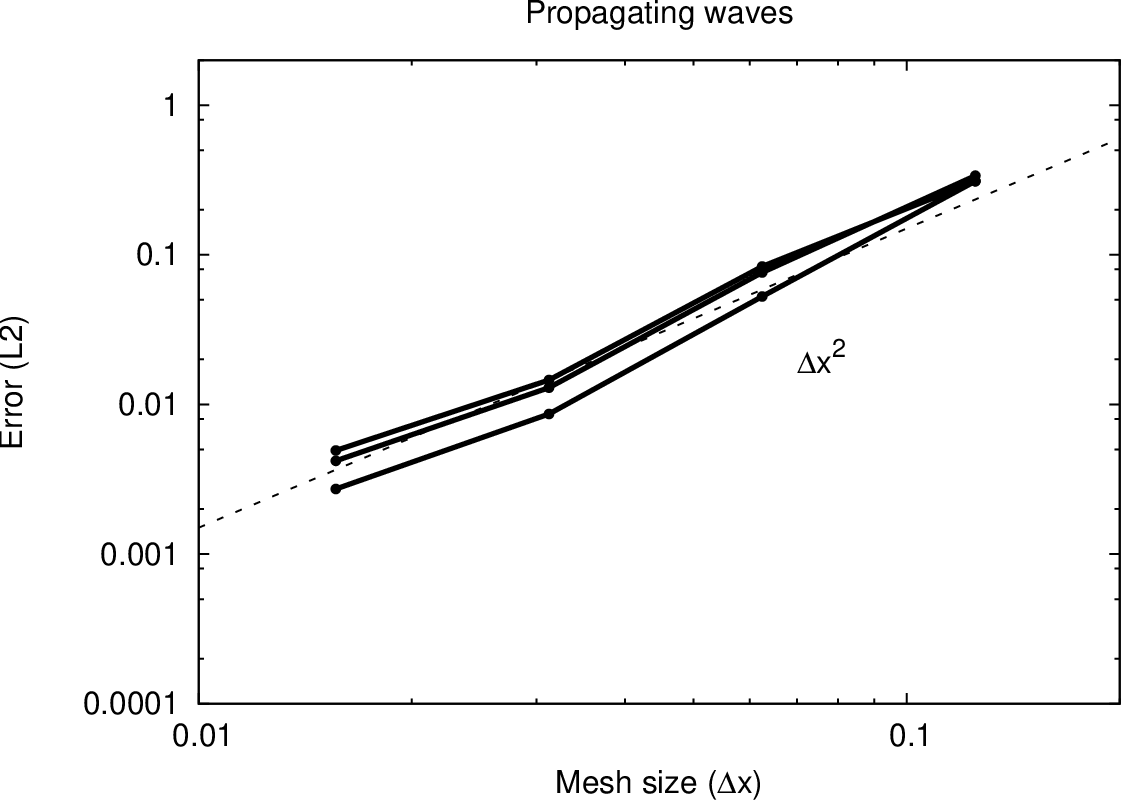
These two expressions for numerical diffusion ( for propagating waves, and for standing waves) are representative of the real diffusion, as confirmed by the study of the evolution of the error (Figure 10).

To take into account this numerical diffusivity, we solve again the equations of induction (Equation 63) and momentum (Equation 62) for a dispersion equation with an additional (numerical) diffusion:
| (80) | ||||
| (81) |
yield
| (82) |
As we have restricted the numerical effect to a diffusion, there is no contribution to the imaginary part of the pulsation, as can be seen in Equation (82).
The propagating Alfvén waves test
We start the simulation with an initial perturbed state with , , , and and , where denotes the real part of a complex number. For the propagating wave test, we have chosen our initial conditions so that .
The internal energy equation (see Shu [31]) can be written as:
| (83) |
In the case of perfect gases, we have . Since Alfvén waves are transverse waves, and . The energy equation thus reduces to
| (84) |
. This last equation, combined with our choice , gives .
Using Equation (84), the time evolution of the pressure writes
| (85) |
Figure 11 shows profiles of , , , , and along the direction after three wave periods (i.e, ), for , with a fully refined grid using 32 cells. The solid line represents the analytical solution. The agreement between the numerical and the analytical solution is excellent (see the amplitude of the error on the figure), even after the wave amplitude has decreased by a factor of about 2.
In order to check for the numerical diffusion as explained in Equation (82) we need to perform the same simulation using less cells for the numerical diffusivity () to be not negligible compared to the physical diffusivity (). The profiles of , , and along the direction after five wave periods (i.e, ) for with a grid of 16 cells is represented Figure 12. The solid lines represent the analytical solutions either without taking into account the numerical diffusivity (the not corrected curves), or correcting the damping factor according to Equation (82) (the corrected curves). The agreement between the numerical and the analytical solution taking into account numerical diffusivity is excellent (see the amplitude of the error on the figure).


The standing Alfvén waves test
We now start the simulation from an initial perturbed state obtained by adding two propagating waves in opposite directions with the same damping , and let the system evolve. Figure 13 displays a snapshot of the evolution of , , , , and along , after about 4 periods (in order for and to be greater than zero) for . The excellent agreement between the numerical and the analytical solution is confirmed.
As previously, we determine the time evolution of the pressure thanks to Equation (84)
| (86) |


Following Choi et al. [7] it is interesting to study the time variation of the magnetic field in the direction, , as represented Figure 14. The analytical solution is represented by the solid line while the dotted line represents the error and the squares the simulation.

II.4.4 Convergence order
We tested the evolution of the precision of the implementation of ambipolar diffusion by examining the evolution of the error with the level of refinement, i.e with the mesh size , for Alfvén standing waves and the Barenblatt test. The error is defined here as the maximum difference between the analytical values and the numerical solution, corrected by the damping factor for Alfvén waves. The error against the cell size follows a power-law, at least in the range studied here (up to 10 periods of the wave). For the standing waves we find
| (87) |
For the Alfvén propagating waves
| (88) |
For the Barenblatt test
| (89) |
A log-log plot of the error as a function of cell size for different times is shown on Figure 10 for Alfvén standing waves and propagating waves, and on Figure 7 for the Barenblatt test. Note that the evolution of the error follows the power laws found through the modified equation study, in Section II.4.3.
II.4.5 Estimate of the numerical drift coefficient of ambipolar diffusion
As seen in § II.4.3, the dissipation of Alfvén waves is slightly larger than expected according to the analytical values. The spurious dissipation due to the numerical scheme can be estimated as:
| (90) |
where is the value measured in the numerical simulation, with , and is the drift contribution due to numerical dissipation. Another way to proceed is to set , to examine how the Alfvén waves dissipate, and then to estimate as . Both methods give about the same value for . For a level of AMR refinement of , we get ; for , and for , , to be compared with or 0.033 for the present simulations. As expected, the better the resolution, the smaller the numerical diffusion.
Figure 15 is a plot of the dissipation of Alfvén waves with , as explained previously. The red solid line corresponds to the analytical solution corrected with our estimate of the magnitude of the numerical diffusion, as explained in Equation (82), while the black solid line corresponds to the uncorrected analytical solution (no diffusion).

III Ohmic diffusion
III.1 Equations
We now turn to the case of Ohmic diffusion in the MHD equations. Equations (1), (2), (5) and (8) remain the same. The energy equation is now:
| (91) |
where and denote the total energy and pressure:
| (92) | |||
| (93) |
The time evolution of reads:
| (94) |
The Lorentz force and the Ohmic diffusivity EMF read:
| (95) | ||||
| (96) |
where denotes the Ohmic diffusivity.
III.2 Computation of Ohmic diffusivity
Various authors (Machida et al. [21], Machida et al. [22], Machida et al. [23], Machida et al. [24]) have studied the influence of Ohmic diffusion, in particular in the context of molecular cloud’s collapse. Their work assumes that the heating from Ohmic resistivity is negligible, and that the approximation is valid. We choose a more general framework and do not assume either of these two assumptions. We implement in RAMSES non-isothermal Ohmic diffusivity, with the exact EMF
To compute the term of Ohmic diffusivity we proceed exactly as in § II.2.1.
III.2.1 The Ohmic diffusion EMF
III.2.2 The Ohmic diffusion energy flux
III.2.3 Computation of the time step in presence of Ohmic diffusion
The characteristic Ohmic diffusivity time step, , is computed according to
| (98) |
where, as for the ambipolar diffusion case, the coefficient 0.1 yields a small enough time step to ensure good code convergence. The computational time step is the minimum between and the time step obtained for the ideal MHD case.
III.3 Tests for the Ohmic diffusion
III.3.1 Test of Ohmic diffusivity alone
We first examine the accuracy of the treatment of Ohmic diffusivity alone. We take exactly the same conditions as in § II.4.1 for ambipolar diffusion. We further assume that is constant. In that case the induction equation reduces to a diffusion equation with a constant diffusion coefficient, using the divergence-free condition :
| (99) |
The solution to this equation for an initial state given by a Dirac pulse is the well known heat diffusion equation which yields a gaussian distribution with a width spreading as . This can easily be studied either for a one dimensional pulse (e.g. , , ) or a two dimensional pulse (e.g. , , ). The results (setting ) are displayed on Figure 16. The agreement between the numerical and the analytical results is excellent, always better than about 0.5%. We checked that the results obtained on an AMR grid are as good as the ones obtained on a regular grid corresponding to the highest level of refinement, and that exactly the same results are obtained for any orientation of the magnetic field.
The evolution of the error as a function of the resolution is represented Figure 17. For this particular test (heating equation) the spatial scheme is of order 2: .


In this case, due to the smoothly varying magnetic field, using a refinement strategy based on is not very efficient: the AMR runs are using typically the same number of cells as a fully refined grid (at least for our tests between level 5 and 9).
III.3.2 C-shock
Proceeding as in § II.4.2 we have tested the accuracy of our treatment of Ohmic diffusivity for the case of an oblique C-shock. For a stationary shock in the direction (all quantities are supposed to only depend on ) the equations of mass, momentum, energy, magnetic field conservation and the condition read:
| (100) | ||||
| (101) | ||||
| (102) | ||||
| (103) | ||||
| (104) | ||||
| (105) |
This set of equations is solved numerically and provides the benchmark to which the simulation with the RAMSES code will be compared to assess the accuracy of the numerical treatment in the code.
We start from a steep function as initial state for the different variables whose values are the ones taken at infinity ahead of and behind the shock, respectively, in the frame of the shock. These values are displayed in Table 2. For this test the Ohmic diffusivity coefficient is set to . The results are portrayed on Figure 18. As seen in the figure, after a transitory regime the shock becomes stationary, as expected. A very small drift velocity of the shock front persists, of the order of 0.25% of the minimum value of . Identical results are obtained for any orientation of the magnetic field and of the initial velocity.


| Variable | ||||||
| Pre-shock value | 0.4 | 3 | 0 | 0.4 | ||
| Post-shock value | 0.71084 | 1.68814 | 0.4299 | 1.43667 | 1.19222 |
Such an agreement between the numerical and the analytical solutions, within about 0.2% (except a few points where it can reach 1%) can be considered as very satisfactory and asseses the validity of our treatment when hydrodynamics and Ohmic diffusion are coupled.
The grid is refined if the gradient of magnetic field, pressure, density or velocity is greater than 0.1 (this insures for this test that the error on the AMR grid and on the regular grid are about the same).
III.3.3 Alfvén waves
Proceeding as for the ambipolar diffusion study we have examined the behaviour of propagating Alfvén waves as well as of standing waves in an non-isothermal ionized plasma in the case of Ohmic diffusion. Lesaffre and Balbus (2007) derived analytical solutions for the general case of MHD flows with shear, non-zero resistivity , viscosity and cooling. In the absence of shear and rotation, these authors showed that torsional Afvén waves are a solution for such flows.
Following closely the notations of Lesaffre and Balbus (2007), the unperturbed state in both studies for a wave propagating in the direction is defined as:
For the propagating wave study, the perturbed state is chosen such as and (we necessarily have ). Furthermore, we have (constant density), but the pressure varies with time, so that (see Lesaffre & Balbus 2007). In the absence of shear, viscosity and rotation, the relation between the perturbed magnetic field, , and the perturbed velocity, , reads
| (106) |
with the wave angular frequency and the wave number.
The time evolution of the gaz pressure is governed by the equation:
| (107) |
with the adiabatic coefficient of the gaz and the current.
Since only depends on and has components only in the and direction, . We finally get
| (108) |
The solutions of the dispersion relation read:
| (109) |
with . A value yields a moderate damping, with and , whereas a value produces a stronger damping, with and .
Estimating numerical diffusion
Proceeding exactly as in § II.4.3 we can derive the leading order error term in the ideal MHD scheme for Alfvén standing, and propagating waves.
Propagating waves
We start the simulation from an initial perturbed state with and . The time evolution of the pressure is:
| (110) |
For the propagating wave test, we have arbitrarily chosen and let the system evolve from the initial state. Figure 19 portrays a snapshot of the evolution of , , , , and along the -direction after five wave periods (i.e, ), for . Once again, the agreement between the numerical and the analytical solution is very satisfactory, at most of the order of a few percents.


Standing waves
As for the ambipolar diffusion, we start the simulation from an initial perturbed state obtained by adding two propagating waves with opposite values of and the same value of , and let the system evolve. The evolution of the pressure is (in real notation):
| (111) |
Figure 20 shows a snapshot of the evolution of , , , , and along after three wave periods ( ), for . As seen, once again, the agreement between the numerical and the analytical solution is very good, of the order of or better than a few percents.


III.3.4 Convergence order
We tested the evolution of the precision of the implementation of Ohmic diffusion by examining the evolution of the error with the level of refinement, i.e with the mesh size for Alfvén standing waves and the Barenblatt test. The error is defined here as the maximum difference between the analytical values and the numerical solution, corrected by the damping factor for Alfvén waves, and the error at the center of the box for the Barenblatt test. The error as function of cell size follows a power-law, at least in the range studied here (up to 10 periods of the wave). For the standing waves we find:
| (112) |
For the Alfvén propagating waves
| (113) |
For the Barenblatt test
| (114) |
A log-log plot of the error as a function of cell size for different times is given on Figure 22 for Alfén standing waves, and on Figure 17 for the barenblatt test. The behavior of the error for the propagating waves differs if the mesh size is coarse or fairly refined ( or respectively). For the Barenblatt test, the error scales as . In the case of Ohmic diffusion, Equation (99) reduces exactly to the Heat equation, whereas in the case of ambipolar diffusion, Equation (54) reduces to a non-linear diffusion equation. The error in the two cases scales as .


III.3.5 Estimate of the numerical drift coefficient of Ohmic diffusion
As seen in Section III.3.3, the dissipation of Alfvén waves is slightly larger than expected according to the analytical values. The spurious dissipation due to the numerical scheme can be estimated as:
| (115) |
where is the value measured in the numerical simulation, with , and is the drift contribution due to numerical dissipation. Another way to proceed is to set , to examine how the Alfvén waves dissipate, and then to estimate as . Both methods give about the same value for . For a level of AMR refinement of 4, we get ; for 5, and for 6, , to be compared with or 0.02 for the present simulations. As expected, the better the resolution, the smaller the numerical diffusion.
IV Conclusion
In this paper we have described a numerical method to implement the treatment of the two important terms of non-ideal MHD, namely ambipolar diffusion and Ohmic dissipation, into the multi-dimensional AMR code RAMSES. For ambipolar diffusion, we have used a single fluid approach, which is valid when the Lorentz force and the neutral-ion drag force are comparable, corresponding to a domain of strong coupling between the fluid and the field lines. The situations where such an approximation can be made are numerous, of which cloud collapse or certain protoplanetary disks are two typical examples. The accuracy of our numerical resolution of the MHD equations was examined by performing a diversity of tests, for which either analytical or benchmark solutions exist. For both ambipolar and Ohmic diffusion, we first explored the purely magnetic case, without any coupling to the hydrodynamics. For ambipolar diffusion, this was done by comparing the evolution of a Dirac pulse to the solution provided by Barenblatt while for Ohmic diffusion, the solution is confronted to the well known heat diffusion equation. In a second step, we studied the full MHD case (coupling the fluid to the magnetic field) by considering first an oblique shock, and then the behavior of propagating and standing Alfvén waves. For all these tests the solutions obtained with our method show excellent agreement with the analytical predictions, typically within a few tenths of a percent on average, showcasing the validity and the robustness of our method. We have also carefully analyzed the main source of numerical error using the Modified Equation framework. In order to estimate the spatial resolution that is required to model non-ideal MHD effects reliably. This opens the avenue to a vast domain of astrophysical applications, in particular cloud collapse, pre-stellar core formation and protostellar disks where ambipolar and Ohmic diffusion processes are believed to play a dominant role. Such astrophysical applications of the non-ideal MHD equations with RAMSES will be explored in forthcoming papers.
Acknowledgement
The research leading to these results has received funding from the European Research Council under the European Community’s Seventh Framework Programme (FP7/2007-2013 Grant Agreement no. 247060)
Appendix A The Barenblatt-Pattle solution
Following Grundy & McLaughlin [13], the solution of Equation (54) in general form (), where depends on the problem, is:
| (A1) |
With the dimensionality of the problem, the various constants are defined as follow:
| (A2) | ||||
| (A3) | ||||
| (A4) | ||||
| (A5) |
Appendix B Semi-analytical solution for the isothermal C-shock
Following Mac Low et al. [20], in the isothermal case with a constant ion density, we reduce the set of MHD equations to:
| (B1) | ||||
| (B2) | ||||
| (B3) | ||||
| (B4) |
with and derived from the initial state, the Alfvén Mach number, and the Mach number; is the angle between the magnetic field and the velocity field; and and are the dimensionless density and magnetic field.
Appendix C Semi-analytical solution for the non-isothermal C-shock
Following Duffin & Pudritz [9] and Wardle [40], and reminding that the set of equations is not exactly the same as ours, we solve the set of equations:
| (C1) | ||||
| (C2) | ||||
| (C3) | ||||
| (C4) | ||||
| (C5) | ||||
| (C6) |
where the dimensionless quantities are , , the velocities , . and are the initial dimensionless pressure and magnetic fields, is the angle between the pre-shock velocity and the magnetic field, and the Alfvén Mach number.
References
- [1] Alexiades, V., Amiez, G., & Gremaud, P. A. 1996, Communications in Numerical methods in engineering, 12, 31
- [2] Balsara, D. S. 1996, Astrophys. J. , 465, 775
- [3] —. 2001, Journal of Computational Physics, 174, 614
- [4] Basu, S. & Ciolek, G. E. 2004, Astrophys. J., Lett. , 607, L39
- [5] Basu, S. & Dapp, W. B. 2010, Astrophys. J. , 716, 427
- [6] Black, D. C. & Scott, E. H. 1982, Astrophys. J. , 263, 696
- [7] Choi, E., Kim, J., & Wiita, P. J. 2009, Astrophys. J., Suppl. Ser. , 181, 413
- [8] Dapp, W. B. & Basu, S. 2010, A&A , 521, L56+
- [9] Duffin, D. F. & Pudritz, R. E. 2008, MNRAS , 391, 1659
- [10] Elmegreen, B. G. 1979, Astrophys. J. , 232, 729
- [11] Falle, S. A. E. G. 2003, MNRAS , 344, 1210
- [12] Fromang, S., Hennebelle, P., & Teyssier, R. 2006, A&A , 457, 371
- [13] Grundy, R. E. & McLaughlin, R. 1982, Proc. R. Soc. Lond., 383, 89
- [14] Hennebelle, P. & Teyssier, R. 2008, A&A , 477, 25
- [15] Khokhlov, A. 1998, Journal of Computational Physics, 143, 519
- [16] Krasnopolsky, R., Li, Z., & Shang, H. 2010, Astrophys. J. , 716, 1541
- [17] Kunz, M. W. & Mouschovias, T. C. 2009, Astrophys. J. , 693, 1895
- [18] Lesaffre, P. & Balbus, S. A. 2007, MNRAS , 381, 319
- [19] Li, Z.-Y., Krasnopolsky, R., & Shang, H. 2011, ArXiv e-prints
- [20] Mac Low, M., Norman, M. L., Konigl, A., & Wardle, M. 1995, Astrophys. J. , 442, 726
- [21] Machida, M. N., Inutsuka, S., & Matsumoto, T. 2006, Astrophys. J., Lett. , 647, L151
- [22] —. 2007, Astrophys. J. , 670, 1198
- [23] —. 2008, Astrophys. J. , 676, 1088
- [24] —. 2009, Astrophys. J., Lett. , 704, L10
- [25] Machida, M. N., Matsumoto, T., Tomisaka, K., & Hanawa, T. 2005, MNRAS , 362, 369
- [26] Mellon, R. R. & Li, Z. 2009, Astrophys. J. , 698, 922
- [27] Mestel, L. & Spitzer, Jr., L. 1956, MNRAS , 116, 503
- [28] Nakamura, F. & Li, Z. 2008, Astrophys. J. , 687, 354
- [29] O’Sullivan, S. & Downes, T. P. 2006, in Astronomical Society of the Pacific Conference Series, Vol. 359, Numerical Modeling of Space Plasma Flows, ed. G. P. Zank & N. V. Pogorelov, 178
- [30] Pinto, C., Galli, D., & Bacciotti, F. 2008, A&A , 484, 1
- [31] Shu, F. H. 1992, Journal of the British Astronomical Association, 102, 230
- [32] Shu, F. H., Lizano, S., & Adams, F. C. 1987, in IAU Symposium, Vol. 115, Star Forming Regions, ed. M. Peimbert & J. Jugaku, 417–433
- [33] Stone, J. M. & Norman, M. L. 1992, Astrophys. J., Suppl. Ser. , 80, 753
- [34] Teyssier, R. 2002, A&A , 385, 337
- [35] Teyssier, R., Fromang, S., & Dormy, E. 2006, Journal of Computational Physics, 218, 44
- [36] Tilley, D. A. & Balsara, D. S. 2008, MNRAS , 389, 1058
- [37] —. 2011, MNRAS , 415, 3681
- [38] Toth, G. 1994, Astrophys. J. , 425, 171
- [39] Toth, G. & Roe, P. 2002, Journal of Computational Physics, 180, 736
- [40] Wardle, M. 1991, MNRAS , 251, 119