Satellites of Legendrian knots and representations of the Chekanov–Eliashberg algebra
Abstract.
We study satellites of Legendrian knots in and their relation to the Chekanov–Eliashberg differential graded algebra of the knot. In particular, we generalize the well-known correspondence between rulings of a Legendrian knot in and augmentations of its DGA by showing that the DGA has finite-dimensional representations if and only if there exist certain rulings of satellites of the knot. We derive several consequences of this result, notably that the question of existence of ungraded finite-dimensional representations for the DGA of a Legendrian knot depends only on the topological type and Thurston–Bennequin number of the knot.
1. Introduction
The satellite construction in knot theory produces new knot types from a given knot by considering the image of a solid torus knot (or link) inside a tubular neighborhood of . This construction provides a simple template for producing whole classes of knot invariants of since we can simply apply existing invariants to the various satellites of . As a well-known example, when this scheme is applied to the Jones polynomial, the associated class of satellite invariants are typically organized into a sequence of so-called colored Jones polynomials. This wider collection of invariants generalizes the Jones polynomial to a family of quantum invariants obtained by labeling by an arbitrary irreducible representation.
An analog of the satellite construction exists for Legendrian knots in with its standard contact structure. In this setting, a Legendrian satellite arises from a Legendrian pattern, , and a Legendrian companion, , where denotes the -jet space of . In this article, we study the effect of this Legendrian satellite operation on a pair of related invariants of Legendrian knots, the ruling polynomials, and the Chekanov–Eliashberg differential graded algebra (DGA). All of the relevant definitions are recalled in Section 2.
A well-known result [5, 6, 17] in Legendrian knot theory asserts that for a Legendrian knot , the existence of a normal ruling of the front projection of is equivalent to the existence of an augmentation of the Chekanov–Eliashberg DGA of . (See Theorem 2.24 below.) In addition, a relationship between ruling polynomials and the Kauffman and HOMFLY-PT knot polynomials ([15], see Theorem 2.14 below) shows that for either of these conditions to hold, the Thurston–Bennequin number of must be maximal. Moreover, the existence of - or -graded augmentations or normal rulings depends only on the Thurston–Bennequin number and topological knot type of . In this article, we present generalizations of these results to finite-dimensional representations of the Chekanov–Eliashberg algebra (where an augmentation is simply a -dimensional representation) and certain normal rulings of Legendrian satellites of .
To give a more precise overview of our main results, we introduce some notation. Denote the Chekanov–Eliashberg differential graded algebra of over by . In our notation, refers to a chosen base point on which corresponds to a distinguished algebra generator measuring homology classes in . Given a divisor of twice the rotation number of , a -graded representation of consists of a -graded vector space together with a homomorphism of differential graded algebras . The requirements here are that and preserves grading mod . See Definition 2.26 below.
In Theorem 4.8 we provide necessary and sufficient conditions for the existence of -graded representations of of any fixed graded dimension in terms of so-called normal rulings of certain satellites of (see Section 2.5 for the definition of normal ruling). We can give a particularly simple statement in the special case of -graded representations:
Theorem 1.1 (cf. Theorem 4.8).
Let be a Legendrian knot. Then the DGA admits a -graded representation of dimension if and only if the satellite of with an -stranded Legendrian full twist, , has a normal ruling.
Topologically, the satellite in Theorem 1.1 is the -component link given by parallel copies of with respect to framing coefficient . We also generalize Theorem 4.8 to give an explicit relation between satellites with more general patterns than and representations of the DGA of particular sorts; see Theorem 4.7.
In order to prove Theorems 1.1 and 4.7, we need to study normal rulings of general Legendrian satellites in terms of the pattern and companion , and this is an interesting subject in its own right. Many normal rulings of a satellite do not reflect any significant aspect of . Indeed, an explicit construction (Theorem 3.4 below) shows that any normal ruling of the pattern may be extended to a normal ruling of , so the satellite always has at least as many normal rulings as . (See Corollary 3.5.) If happens to have more normal rulings than we say that is -compatible. The question of existence of normal rulings of then naturally generalizes to the question of -compatibility. This turns out to be related to the existence of representations of : has a finite dimensional representation if and only if we can find a pattern such that is -compatible, and for particular we can classify which sorts of representations of are equivalent to -compatibility. The approach here is to reduce from the case of an arbitrary pattern to the case when is a product (disjoint union) of particularly simple patterns called basic fronts. See Theorems 4.7 and 4.11.
We also extend other results regarding augmentations and rulings to the setting of finite-dimensional representations. For instance, we have the following generalization of the result that the existence of an augmentation of the DGA implies maximal Thurston–Bennequin number and depends only on topological knot type and :
Theorem 1.2 (cf. Theorem 4.9).
If the DGA has an (ungraded) finite-dimensional representation, then maximizes within its topological knot type. Furthermore, the existence of such a representation depends only on and the topological type of .
This result again makes use of the connection with the Kauffman and HOMFLY-PT polynomials as in the work of the second author [15]. There is also a relation to a conjecture by the first author [11] about the topological invariance of the so-called abelianized characteristic algebra; see Section 4.2.
We note that there are examples of Legendrian torus knots with maximal that admit -dimensional representations but not -dimensional representations. This was observed by Sivek in [19]; the question of existence of finite dimensional representations was raised in the same article, and is discussed in this context in Section 5. At this time, it is an open question if there are knots that admit -dimensional representations but have no representations of dimension or .
Remark 1.3.
Our work indicates that in a certain concrete way, information about the DGA of various satellites of is already encoded in the Chekanov–Eliashberg algebra of itself, though in an algebraically complicated manner. (By comparison, note e.g. that the colored Jones polynomials for a smooth knot are not determined by the Jones polynomial.) For example, Theorem 1.1 shows that augmentations of the satellite of with a full twist correspond to -dimensional representations of . It is interesting to ask how much this situation persists to the plethora of other invariants derived from . For instance, can the collection of linearized homology groups of satellites of be recovered from ?
We conclude this section by outlining the rest of the paper. In Section 2, we recall necessary background about the satellite construction, normal rulings, and the Chekanov–Eliashberg algebra. Section 3 focuses on normal rulings of satellite links. A restricted class of reduced normal rulings is introduced as they have a particularly close connection with representations of .
Section 4 contains theorems connecting finite-dimensional representations and normal rulings of satellites, including most of the results discussed in this introduction. Our most precise result, Theorem 4.7, gives, in the case of a pattern without cusps, an equivalence between the existence of reduced rulings of and finite dimensional representations of in which the distinguished generator has matrix related to the path matrix of introduced by Kálmán [8].
Finally, Section 5 provides a detailed treatment of a special case, the question of existence of -dimensional representations (with particular restrictions on the image of ). A sufficient condition for -compatibility is given in Theorem 5.4, and the case of knot types with or fewer crossings is addressed completely.
Acknowledgments
We thank Brad Henry, Steven Sivek, and Michael Sullivan for interesting conversations related to this work. The first author was partially supported by NSF CAREER grant DMS-0846346. The second author thanks the Max-Planck-Institut für Mathematik in Bonn for providing an excellent research atmosphere during a portion of this work.
2. Background
In this section, we give background on Legendrian links in and , the Legendrian satellite construction, normal rulings, the Chekanov–Eliashberg differential graded algebra, and assorted other constructions that will be necessary for the remainder of the paper.
2.1. Legendrian links
We consider Legendrian links in and in an open solid torus with the contact structure provided in either case by the kernel of . From the point of view of contact geometry, these spaces are perhaps more naturally viewed as the -jet spaces of the line and circle respectively. Correspondingly, we will usually use to denote with this contact structure.
A Legendrian link in a -jet space can be recovered from its image in under the projection ; this image is referred to as the front projection or front diagram of . We will use the same notation for a link and its front diagram, but will point out the distinction when necessary. In the case when , the -coordinate is circle-valued, so the front projection is a subset of an annulus. We write this annulus as with the lines and identified, and we will often view the front projection of a Legendrian link in as a subset of .
Generically, front projections are unions of closed curves in the -plane or annulus which are immersed away from semi-cubical cusp singularities and one-to-one except for transverse double points. In addition, vertical tangencies cannot occur. Conversely, any collection of curves of this type lifts to a Legendrian link. Two Legendrian links, and , are Legendrian isotopic if there is a smooth isotopy, , connecting them with Legendrian for all . The Legendrian isotopy may always be chosen so that the front projections of the are generic except for a finite number of Legendrian Reidemeister moves; see Figure 1. A Legendrian isotopy of this type will be referred to as a generic isotopy.

A Legendrian link has a framing arising from the contact structure. There is a Legendrian isotopy invariant which equals the corresponding framing number in the case that is null-homologous. In general, we define via a generic front projection for by where is the writhe of the projection and is the number of cusps.
For an oriented (connected) Legendrian knot , a second integer-valued invariant, the rotation number , is provided by the winding number of the tangent to around in the contact planes. This is computed from a front diagram as where (resp. ) denotes the number of downward (resp. upward) oriented cusps. For a multi-component link , we will adopt the convention of taking to be the greatest common divisor of the rotation numbers of the components of .
2.2. Maslov potentials
The following additional structure on a front diagram may be viewed as a generalization of an orientation.
Definition 2.1.
Let be a divisor of . A -graded Maslov potential, , for is a function from the front diagram of to which is constant except at cusp points where it increases by when moving from the lower branch of the cusp to the upper branch. See Figure 2. If is even we assume in addition that is even along strands where the orientation of is in the positive -direction.

A -graded Legendrian link is a pair consisting of a Legendrian link with chosen -graded Maslov potential . Maslov potentials may be continued in a canonical way during any of the Legendrian Reidemeister moves. Two -graded Legendrian links , , are Legendrian isotopic if there is a generic isotopy from to which takes to .
We note that for a single-component Legendrian knot , Maslov potentials are unique up to the addition of an overall constant. In fact, more is true: if and are -graded Maslov potentials on , then and are Legendrian isotopic, assuming if is even that and determine the same orientation on . See Remark 2.4.
2.3. Legendrian satellites
The following construction first appears in the literature in [14] where we refer the reader for additional details. Let be an oriented (connected) Legendrian knot with chosen base point, , and a link. Using this information, we form a new link whose Legendrian isotopy type depends only on the Legendrian isotopy types of and . The knot is referred to as the companion; is the pattern; and is the resulting satellite.
Say that is in general position if its front has generic singularities and lies away from these; say that is in general position if its front, viewed as a subset of with ends identified, has generic singularities, all away from . Then we can define diagrammatically.
Let denote the number of intersection points of the front diagram of with the vertical line . We begin by forming a link whose front projection is obtained by taking copies of and shifting the -coordinate of each successive copy downward by a small amount. This link is referred to as the -copy of . Next, we insert the front projection of into the -copy of at the location of the base point. To do this we view the front projection of as a subset of and scale appropriately so that the intersection points of with and line up with the parallel strands in the -copy of . Furthermore, the scaling should be carried out so that does not intersect other parts of the -copy of . If is oriented to the right at then we insert directly into the -copy. However, if is oriented to the left at we instead insert the reflection of across a vertical axis. See Figure 3.
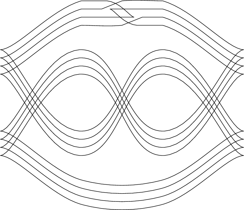
Remark 2.2.
It will often be convenient to have an enumeration of the parallel copies of that make up the satellite. In this article, we adopt the convention of labeling strands of corresponding to a single strand of from to from top to bottom, with the index label increasing as the -coordinate decreases.
If is a common divisor of and , then the choice of -graded Maslov potentials, and , for and gives rise to a -graded Maslov potential, , for as follows. At the location of the base point where is inserted, is the sum of and . Since is connected, this uniquely characterizes . Indeed, let denote the value of on the -th strand of at . Then at the -th strand of corresponding to the point , .
In [14], generic Legendrian isotopies are given to show that the Legendrian isotopy type of depends only on the Legendrian isotopy types of and and, in particular, is independent of the choice of base point . Paying attention to Maslov potentials in the proof shows that the -graded Legendrian isotopy type of depends only on that of and .
Remark 2.3.
The analogous construction for smooth knots requires a choice of framing for in order to produce a satellite whose isotopy type is well defined. If and are Legendrian, such a framing is given by the contact framing for , which has framing coefficient relative to the Seifert framing; thus in this case the smooth knot type of depends only on along with the underlying smooth knot types of and .
Remark 2.4.
As mentioned in Section 2.2, one can use the satellite construction to give an easy proof of the following result.
Theorem 2.5.
Let be a connected Legendrian knot in with two -graded Maslov potentials and , where for some constant , with the additional stipulation that if is even, then is also even. Then and are Legendrian isotopic.

Proof.
It suffices to prove the theorem when , since a general is a multiple of (note that when is odd, every integer is even mod ). If in addition is the standard unknot , then the theorem holds since we can apply two Legendrian Reidemeister I moves, then undo these moves, as shown in Figure 4.
For a general knot , note that can be expressed as a satellite of the unknot, for some : simply perform a Reidemeister I move somewhere along the knot, and then the new loop is the unknot . We can choose Maslov potentials on and so that the Maslov potential on is the sum of these two, in the sense discussed in this subsection. By the theorem for the unknot, there is a Legendrian isotopy on that changes the Maslov potential on by ; then the induced Legendrian isotopy on changes by as well. ∎
2.4. Basic fronts
For , let denote the Legendrian knot whose front diagram is given by identifying the ends of the -stranded braid , where strands are labeled from top to bottom, composition of braids is from left to right, and represent the standard generators of the braid group . That is, is the closure of the -strand front ![[Uncaptioned image]](1206.2259v1/BFront.png) , which winds times around the factor and has crossings. We will refer to the as basic fronts. Moreover, for we write for the basic front
with -graded Maslov potential identically equal to .
, which winds times around the factor and has crossings. We will refer to the as basic fronts. Moreover, for we write for the basic front
with -graded Maslov potential identically equal to .
Given front diagrams , we define their product by stacking above . We introduce some notation for -graded products of basic fronts (see Figure 5 for an illustration). Let be a (finite) sequence of positive integers and a sequence of elements of . Writing for a pair of such sequences, we define as the -graded Legendrian link . Given such a pair , we introduce a function
That is, denotes the total number of strands of a fixed -coordinate with Maslov potential equal to .
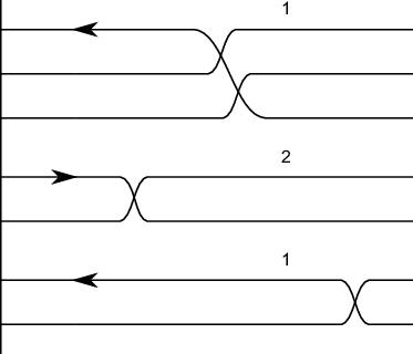
Later, we are able to reduce some questions about satellites with arbitrary pattern to the case where is a product of basic fronts.
2.5. Normal rulings
The notion of normal ruling was developed independently in the works [2, 5]. Let be a Legendrian knot in or whose front projection is generic in the sense described earlier in this section. In addition, we now assume that all crossings and cusps have distinct -coordinates. This can be achieved after a small Legendrian isotopy.
In this section, we unify our notation by viewing . For or , we let denote the projection , where the domain is viewed as the front projection of . Let denote the projection of the set of cusp and crossing points of the front projection of . Furthermore, for any let .
Definition 2.6.
A continuous function from a subset to the front projection of is called a section if .
Definition 2.7.
A normal ruling of the front projection of a link in or is a continuous involution, , , satisfying the following:
- (i)
The involution is fixed point free.
- (ii)
The involution satisfies and therefore restricts to involutions for each .
For a component , the inverse image of in is a union of “strands”, , where each is mapped homeomorphically onto by . Due to the continuity condition, induces an involution of the collection of strands, and we say pairs with if .
- (iii)
In a neighborhood of a cusp point, the involution interchanges the upper and lower branch of the cusp. On the remaining strands, the involution induced by should be the same on either side of the cusp.
- (iv)
Strands meeting at a crossing should not be paired by .
- (v)
The involution extends continuously near crossings in the following sense. If is such that contains a single crossing at -coordinate , then we can find sections such that every point of is in the image of exactly one of the except for the crossing point which is in the image of exactly two of the . Moreover, these sections are preserved by the involution. That is, for any , there exists such that on . It is clear that, except for their enumeration, the sections are uniquely determined by the involution .
At the crossing point, there are two possibilities. Either the two sections that meet at the crossing follow the diagram and cross in a transverse manner, or they each turn a corner at the crossing. In the latter case, we refer to the crossing as a switch of . At a switch, one section covers the upper half of the crossing, and another covers the lower half. Due to requirements (i) and (iv), each of these sections is paired by with a companion strand away from the crossing.
- (vi)
(Normality condition) Near a switch we can produce intervals on the vertical axis by connecting each switching strand with its companion strand. These two intervals should either be disjoint or one should be contained in the other. See Figure 6.

Definition 2.8.
Suppose now that is a -graded Legendrian link. We say that a ruling of is -graded with respect to if for with and , we have mod .
Remark 2.9.
Alternatively, a normal ruling may be viewed as a global decomposition of the front diagram into pairs of sections, and we will make use of this perspective in our figures and proofs. In the case of a link in , it is important here that we view the front diagram as a subset of . Then starting at or at the first left cusp of and working to the right, we can piece together the sections from condition (v). This allows us to cover the front diagram of with a collection of sections with maximal domains of definition. The involution then divides the sections into pairs that begin and end at common cusps or possibly at common components of the boundary of in the case .
Note that in the case , a section that begins at does not necessarily have to end up at the same -coordinate if it makes it all the way to without terminating at a cusp. However, the involution is defined on the front diagram viewed as a subset of , so the overall division of points of into pairs at and should be the same.
For Legendrian links in , it is appropriate for some purposes (see [9]) to relax the fixed point free condition of Definition 2.7 (i).
Definition 2.10.
Let . A generalized normal ruling of is an involution satisfying the requirements of Definition 2.7 except for the following modifications.
- (i)
The involution may have fixed points.
Near crossings, the locally defined sections are no longer uniquely determined by in the case where both of the crossing strands are fixed by . However, if at least one of the crossing strands is not fixed by , then uniqueness still holds. In particular, it is possible to have a switch where one of the switching strands has a companion strand and the other is a fixed point strand. In this case, the normality condition is extended.
- (ii)
(Generalized normality condition) Near switches where one of the strands is fixed by , the vertical interval connecting the non-fixed point strand to its companion strand should not intersect the other strand of the switch. See Figure 7.

Definition 2.8 carries over without change to provide a notion of -graded generalized normal ruling.
Remark 2.11.
A generalized normal ruling produces a decomposition of the front diagram of into pairs of sections and a fixed point subset which does not contain cusps. (Compare Remark 2.9.) We make use of this perspective in our figures.
Given a -graded Legendrian link in or , let (resp. ) denote the set of all normal rulings (resp. generalized normal rulings) of which are -graded with respect to . Finally, we define the -graded ruling polynomial, , by
Chekanov and Pushkar [2] prove the following invariance result.
Theorem 2.12 ([2]).
If and are Legendrian isotopic as -graded links, then .
Remark 2.13.
Note that ruling polynomials are unchanged by the addition of an overall constant to the Maslov potential. In particular, if is a (connected) knot, then the -graded ruling polynomials are independent of the choice of . Moreover, if is an oriented knot, then for any -graded with , the polynomial is a Legendrian isotopy invariant of .
When or the ruling polynomials depend only on the underlying framed knot type of . This follows from:
Theorem 2.14 ([15]).
For any Legendrian link , let denote the Kauffman and HOMFLY-PT link polynomials11 1 We follow here the conventions of [15] for the HOMFLY-PT and Kauffman polynomials. However, our conventions for the power appearing in the ruling polynomial differ by from [15].. Then the -graded (resp. -graded) ruling polynomial (resp. ) is equal to times the coefficient of in (resp. ).
2.6. Chekanov–Eliashberg differential graded algebra
In this subsection we recall the definition of the Chekanov–Eliashberg DGA associated to a Legendrian knot in , with some adjustments (related to base points and commutativity) to adapt the standard treatment to the needs of this paper.
For the purposes of defining the DGA, it is more convenient to work in the Lagrangian () projection than in the front () projection used in the first part of this section. One can use an elementary construction called resolution [11] to produce a Lagrangian projection from a front projection: diagrammatically, smooth out all left cusps, and replace right cusps by a loop with a negative crossing.
Let be an oriented Legendrian knot with a base point , generic in the sense that the Lagrangian projection is immersed with only transverse double points as singularities, and lies away from the double points. Contact homology associates to a differential graded algebra , the Chekanov–Eliashberg algebra, as we now briefly recall; see e.g. [1, 4] for more details.
Definition 2.16.
Label the crossings (double points) of by . The algebra is the associative, noncommutative unital algebra over generated by
with no relations besides .
The algebra is generated as a -vector space by words of the form
(including the empty word, which serves as the identity element ), with multiplication given by concatenation. We note that this definition of is slightly different from the corresponding definition in [4], even accounting for the fact that we work over and not : the algebra considered in [4] is the quotient of ours by allowing powers of to commute with the ’s. This construction follows [12]; see [3, section 2.3.2] for further discussion.
We next give a -grading (and thus a -grading for any ). If is a crossing of , let be a path along beginning at the overcrossing and ending at the undercrossing of . Let be the (non-integral) number of counterclockwise revolutions made by the unit tangent vector to the path from beginning to end, and define . Note that the grading is well-defined, independent of the choice of , modulo . Extend the grading to all of by setting and extending in the usual way (the degree of a product is the sum of the degrees).
If is a resolution of a front diagram endowed with a Maslov potential, then the degree of crossing is the difference of the Maslov potentials associated to the strands passing through . We can also use this to define a grading on the DGA in the more general case where is a multi-component link.
We now come to the differential on . Attach signs to each corner
at every crossing in as
depicted: ![[Uncaptioned image]](1206.2259v1/Reebsigns.png) .
Let denote the closed
disk. For , write , where
are points on appearing in order as
we traverse the boundary counterclockwise.
.
Let denote the closed
disk. For , write , where
are points on appearing in order as
we traverse the boundary counterclockwise.
Definition 2.17.
Let be crossings in the Lagrangian projection of a Legendrian knot . Define to be the space of all orientation-preserving immersions , up to reparametrization, such that:
- •
sends the boundary punctures of to the crossings of
- •
sends a neighborhood of to a corner at labeled by a
- •
sends a neighborhood of each to a corner at labeled by a .
For , the image of maps to a union of paths , where each path begins and ends at a crossing, and goes from to , from to for , and from to . For each of these paths , we can associate a monomial by , where is the number of times passes through the base point , counted with sign according to the orientation of . Finally, we can associate a monomial to , as follows:
Definition 2.18.
Let be a crossing of . The differential is defined by:
where the sum is over all and all choices of crossings such that is nonempty.
We can extend the map to all of by setting and imposing the Leibniz rule.
Theorem 2.19 ([1, 4]).
The map lowers degree by and is a differential: . Up to stable tame isomorphism, the differential graded algebra is an invariant of under Legendrian isotopy (and choice of base point).
Here “stable tame isomorphism” is an equivalence relation of differential graded algebras that in particular fixes and preserves isomorphism type of the homology ; see [1], or [3] for a definition in our setting. For the purposes of this paper, this relation may be treated as a black box.
In Section 4, we will need a slight generalization of the above notion of the Chekanov–Eliashberg DGA, to the setting where we have multiple base points on . As before, we assume that in the projection, no base point coincides with a crossing; we also assume that the base points are cyclically ordered along , i.e., are encountered in that order as we traverse the knot in the direction of its orientation.
Given this data, we define the algebra to be the noncommutative unital algebra over generated by crossings , along with additional generators , with no relations besides for all . (Note in particular that the ’s do not commute with the ’s, or indeed with each other.) We give a -grading as before, with for all .
We can define a differential on analogously to Definition 2.18. Note that in the presence of multiple base points, the monomial associated to a path in can involve any or all of : it is the product , where passes through in succession, and the signs depend on whether the orientation of agrees or disagrees with the orientation of as passes through the base point.
The DGA depends only minimally on the choice of base points, and indeed contains no more information than the single-base-pointed DGA . More precisely, we have the following results.
Theorem 2.20.
Let and denote two collections of base points on , each of which is cyclically ordered along . Let and denote the corresponding multi-pointed DGAs. Then there is a DGA isomorphism such that for all .
Proof.
It suffices to establish the result when and are identical except that for some , is the result of sliding across a crossing of . Suppose then that and lie on opposite sides of a crossing , with the orientation of pointing from to . We first consider the case where the strand containing and is the overstrand at . In this case, if is a disk with a positive corner at and are the words associated to in and respectively, then . Furthermore, if is a disk with a negative corner at , then is the result of replacing by in . It follows that the map defined by , for , and for all satisfies .
If the strand containing and is the understrand at , a similar argument shows that the map defined by , for , and for all satisfies . ∎
Theorem 2.21.
Let be a cyclically ordered collection of base points along , and let be a single base point on . Then there is a DGA homomorphism such that and .
Proof.
By Theorem 2.20, we may assume that all lie in a small neighborhood of . In this case, the map defined by for all crossings and is the desired homomorphism. ∎
2.7. Augmentations and representations of the DGA
Here we discuss representations of the DGA introduced in the previous subsection. We begin with augmentations, which can be viewed as -dimensional representations.
Definition 2.22.
Let . A -graded augmentation of is an algebra map such that:
- •
;
- •
;
- •
if with .
Stable tame isomorphism (discussed briefly in the previous subsection) preserves the existence and nonexistence of -graded augmentations. Theorem 2.19 then immediately implies the following.
Theorem 2.23.
If and are Legendrian isotopic knots with base points and , then for any , the Chekanov–Eliashberg DGA has a -graded augmentation if and only if does.
There is a well-known correspondence between augmentations and rulings:
Theorem 2.24 ([5, 6, 17]).
Let be a Legendrian knot in , and let . Then the front projection of has a -graded ruling if and only if the DGA has a -graded augmentation.
We need the following more precise statement. Recall that a Legendrian link in is said to be in plat position if all right cusps have the same -coordinate as do all left cusps.
Theorem 2.25 ([17, 7]).
Let be a -graded Legendrian link in with front diagram in plat position, and denote by the Chekanov–Eliashberg DGA associated with the resolution of .
- (i)
Given any -graded augmentation of , there exists a -graded normal ruling of so that the first switch of occurs at or to the right of the first augmented crossing.
- (ii)
For any -graded normal ruling of ,there is a -graded augmentation of so that the first augmented crossing agrees with the first switch of .
Proof.
Statement (i) follows from an algorithm in [17, section 3.3] that assigns a normal ruling to an augmentation of a plat position front diagram. This algorithm is also presented in [13], and it is easy to see that the first switch of the normal ruling must be to the right of the first augmented crossing.
For (ii), we cite work of Henry [7]. The main objects of study in [7] are “Morse complex sequences,” which consist of sequences of chain complexes assigned to a front diagram of a Legendrian link in . In [7, section 6.5], two different standard forms for a Morse complex sequence (MCS) are introduced, the -form and the -form. These standard forms are related to normal rulings and augmentations respectively.
Given a normal ruling as in (ii), we consider the -form MCS associated with where none of the returns have handleslides. Theorem 6.20 of [7] shows that this MCS may be transformed into an -form MCS by an algorithm that sweeps handleslide marks from left to right. In particular, the leftmost handleslide in this -form MCS will be located directly to the left of the first switch of . According to Corollary 6.29 of [7], this -form MCS corresponds to an augmentation of the Chekanov–Eliashberg algebra of the resolution of where a crossing is augmented if and only if there is a handleslide immediately to the left of the crossing. This augmentation has the desired form. ∎
We now generalize our discussion from augmentations to representations of the DGA. Suppose is a finite-dimensional vector space over with a -grading, . Then is a -graded algebra where we take each to be homogeneous of degree22 2 Note that with this convention, our definition of degree is the negative of the standard grading for graded linear maps. .
Definition 2.26.
A -graded representation of is a -graded vector space over along with a DGA map from to , i.e., a grading-preserving algebra map satisfying and . The graded dimension of the representation, , is the function defined by
Note that a representation of does not need to send to , but merely to an invertible map on .
3. Normal Rulings of Legendrian Satellites
We begin this section by establishing some basic properties of normal rulings of Legendrian satellites. The definition of normal ruling requires working with a front projection of with the property that crossings have distinct -coordinates. To achieve this, we assume that and are in general position, and then apply a planar isotopy to perturb the -coordinates of the crossings of the front diagram for described in Section 2.3. The precise order that the crossings end up in will not be relevant for our arguments. In this section, we continue to use the convention of labeling the parallel translates of a strand of appearing in from to with decreasing -coordinate.
We introduce some terminology associated with a normal ruling of . Outside of neighborhoods of cusps, crossings, and the base point we can assign an involution, , of to each point according to:
- (i)
Let if, of the parallel copies of in that correspond to the point , the ruling pairs the -th strand with the -th strands, and
- (ii)
let if pairs the -th strand of at with a strand of corresponding to a point other than in .
We will refer to as the thin part of at . In addition, we refer to strands of that correspond to the same strand of and are paired by as a pair of thin strands of .
In combination, the following two lemmas show that the thin part of is independent of .
Lemma 3.1 (Crossing Lemma).
A pair of thin strands cannot be involved in any switches at crossings of that correspond to a crossing of .
Proof.
Let denote the subset of the front diagram corresponding to a neighborhood of a crossing of . We prove the more general statement:
Let and be a pair of companion paths of the ruling. If both, and pass through the region , then neither of them can switch in .
The proof is by induction on, , the number of strands lying in the vertical interval between and at such a switch. The base case of is prohibited by the normality condition. For the inductive step, by symmetry we may assume that lies above and such a switch occurs along .
- Case 1:
The corner along at the switch points toward . Then by the normality condition, the other path at the switch must have its companion path between and . The inductive hypothesis then provides a contradiction.
- Case 2:
The corner along at the switch points away from . Then heading in the appropriate direction, (left or right, depending on the slope of at the switch), and will be on course to intersect within . This is prohibited, so there must be another switch along either or . This next switch will be of the type covered by Case 1, and, prior to this switch, the number of strands between and can only decrease since they are angled toward one another in this direction. Thus, the inductive hypothesis may be applied.
∎
Lemma 3.2 (Cusp Lemma).
The thin part of does not change when passing a cusp. Furthermore, at those crossings of corresponding to a particular cusp of the crossing between the -th strand and the -th strand is a switch if and only if before and after the cusp.
Proof.
By symmetry we may consider the case of a left cusp of . Let denote the corresponding left cusps of numbered from top to bottom. The ruling provides a pair of paths and emanating from each of the where we assume to have larger -coordinate than . Although, it need not literally be the case, we will refer to those strands of which correspond to the upper (resp. lower) branches of cusps as positive (resp. negative) sloped. (Compare Figure 8.)
Claim: Among those crossings near the cusp of , none of the (resp. ) can have a switch where the slope increases (resp. decreases).
This is proved by induction on, , the number of strands lying between and at the offending switch . The base case would violate the normality condition. By symmetry we may assume is a switch along . The normality condition forces that there is some such that (i) the lower half of is an arc along , and (ii) lies above at .
- Case 1:
is positively sloped at . Then immediately to the right of , is negatively sloped and is positively sloped. To the right of , one of these paths must switch or they will intersect before leaving the nearby collection of crossings. However, as we move to the right of the number of strands between and can only decrease, therefore this contradicts the inductive hypothesis.
- Case 2:
is negatively sloped at . This time follow and to the left of . Since they lie between and at , and because of the way they are sloped, one of and must switch in order for them to meet at the cusp . However, the number of strands between and decreases when moving to the left, and thus the inductive hypothesis applies to provide a contradiction at the first such switch.
Finally, we deduce the result from the Claim. Near the cusp, each pair of paths and can have at most one switch combined. Indeed, the claim forbids both and from individually having more than one switch, and if both and have a single switch then they will intersect before leaving the collection of crossings near the cusp. Now, in the case that there is no switch along or , the -th strand will be a fixed point of along either branch of the cusp. Any switches that do occur must have upper strand and lower strand with , and such a switch results in before and after the crossing. Conversely, if before or after the crossing, then a switch of this type is necessary in order for the corresponding thin strands to meet at a common cusp. ∎
3.1. Reduced normal rulings
Definition 3.3.
For a non-empty pattern , we say that a normal ruling is reduced if
- (i)
the front projection of intersects and
- (ii)
there are no switches at the crossings of which arise from left cusps of .
Denote by the set of reduced -graded normal rulings of and by the corresponding reduced ruling polynomial. When we make the convention that the empty ruling is reduced so that contains a single element.
Any normal ruling of corresponds to a generalized normal ruling of along with a reduced normal ruling of a certain satellite associated to . More precisely, we have the following.
Theorem 3.4.
Assume that and have front diagrams in general position. There is a bijection where is the set of ordered pairs satisfying and . Here, denotes the link whose front diagram corresponds to the portion of that is fixed by . Furthermore, , and is -graded if and only if and are.
Proof.
Given a pair , is constructed as follows.
- Step 1.
Extend to a partial ruling, of with some fixed point strands:
This is done by letting along the subset and then extending so that away from cusps the thin part of agrees with the involution at the boundary of the front projection of in . That is, except near cusps, the -th and -th parallel copies of a strand of in are paired by if and only if on the vertical line , . All other strands of are fixed point strands for . Finally, to piece together, for each such and we add one switch at every cusp. Assuming , these switches occur where the -th strand corresponding to the lower branch of the cusp passes over the -th strand. See Figure 8.

Figure 8. The thin part of a ruling of near cusps. - Step 2.
Extend to :
The fixed point strands of (after smoothing near any relevant switches within ) form a front diagram which is combinatorially the same as . We extend by requiring that the restriction to is the normal ruling . See Figure 9.
The switches of can be divided into three disjoint types: (A) Switches of , (B) switches of , and (C) switches near cusps added in Step 1.

The normality condition is easily verified for switches of type (B) and (C). For switches of type (A) we need to consider two subcases. If neither of the involved strands are fixed point strands of , then the normality condition follows since it holds in . If one of the switching strands, say , is a fixed point strand of , then the normality condition for the ruling follows from the generalized normality condition for provided that we know the companion strand of in lies outside of . This is true for the following reason. The fixed point subset, , cannot contain cusps, so if their are a pair of thin strands of within the subset , then we will continue to have a pair of thin strands immediately to the left of . Following this strand of to the left the Crossing Lemma implies that we continue to have a pair of thin strands until we reach a left cusp of . Finally, the Cusp Lemma then contradicts the assumption that is a reduced ruling of .
Next, we verify that . The cusps of not belonging to the subsets and are in two-to-one correspondence with switches of type (C). Recall that the negative term of counts the total number of cusps. Thus, in the computation of switches of type (C) precisely cancel these unclaimed cusps and we are left with . (Here, we used that does not contain cusps, so that none of the cusps of are double counted in .)
Now we check that is -graded if and are. In the construction the only paired paths of that do not belong to either or are the thin pairs arising from Step 1. Clearly, immediately next to the requirement of Definition 2.8 continues to hold. Following along , it is enough to verify that the condition continues to hold for thin pairs after passing a cusp. This is immediate. Near cusps, thin pairs belonging to the upper and lower branch of the cusp are in correspondence, and the Maslov potentials differ by .
Finally, we show that is onto. Let be arbitrary. The restriction of to produces a generalized normal ruling by making the convention that strands of mapped outside of by are fixed point strands of . The cusp and crossing lemmas imply that the thin part of is constant and that, precisely as in the construction from Step 1, the only switches outside of involving thin strands are near cusps of . Moreover, the complement of the thin strands of will be precisely and restricting to this subset produces such that . ∎
Corollary 3.5.
For any Legendrians and with -valued Maslov potential, we have
where refers to inequality between all coefficients of corresponding powers of .
Proof.
This follows from Theorem 3.4 and the injection sending , where is the unique element of . ∎
3.2. Normal rulings of satellites and the Thurston–Bennequin number
Corollary 3.5 suggests the following definition.
Definition 3.6.
Let be a Legendrian knot and a Legendrian link, each equipped with a -valued Maslov potential. Then is -compatible if .
In this subsection, we discuss a correlation between -compatibility and maximal Thurston–Bennequin number; later we show that -compatibility is related to the existence of representations of the Chekanov–Eliashberg DGA.
Recall that a Legendrian knot has positive and negative stabilizations and obtained by inserting a pair of consecutive cusps (a zigzag) into a strand of the front projection of . The stabilization is positive (resp. negative) if the new cusps have the orientation of running downward (resp. upward) along the cusp. The Legendrian isotopy type of depends only on the Legendrian isotopy type of , and any Legendrian that is isotopic to for some is said to be stabilized.
Remark 3.7.
- (i)
Stabilization may be viewed as a special case of the Legendrian satellite construction since where are pictured in Figure 10.
- (ii)
Note that .
Theorem 3.8.
If is stabilized, then for any nonempty with any choice of Maslov potential, , i.e., is not -compatible.
Proof.
We may assume that and are in general position; that the front diagram of contains a zigzag; and that the base point does not lie on the strand, , that connects the two cusps of the zigzag. On the front diagram of the satellite , let and denote the left and right cusps corresponding to the zigzag on .
Let be a normal ruling of . We will show that along the thin part of , , does not have fixed points. Consider the ruling paths and originating at a cusp . If switches before leaving the crossing near the , then it follows from the Cusp Lemma that . If not, then must end at one of the . Then would need to end at as well, but this ensures that must switch at one of the crossings near the . Again, the Cusp Lemma shows that .
Now, from the Cusp and Crossing Lemmas we see that the thin part of must be fixed point free everywhere. In particular, restricts to a normal ruling, , (without fixed points) on . It follows that . Thus, the injection of from Corollary 3.5 composed with is onto , and the result follows. ∎
Corollary 3.9.
If there exists a pattern such that is -compatible, then is maximal within the smooth knot type of .
Proof.
If is non-maximal, then there exists a stabilized knot with the same smooth type as and . Then
where the first equality is a combination of Remark 2.3 with Theorem 2.14 and the second is Theorem 3.8.
If is -compatible where has a -graded Maslov potential, then it remains -compatible in the ungraded setting. This contradicts . ∎
3.3. Reduced ruling polynomials
Theorem 3.4 shows that
| (1) |
We will use this relation to deduce properties of reduced ruling polynomials from corresponding results about standard ruling polynomials.
Theorem 3.10.
Let be a Legendrian knot with . For any fixed -graded with generic front projection, is a Legendrian isotopy invariant of .
Proof.
First we establish the result for those front projections that do not have cusps. In this case, the summation on the right side of (1) contains (when is the generalized ruling that fixes every strand of ). The remaining terms on the right hand side are a -linear combination of reduced ruling polynomials of the form where is again a front projection without cusps and fewer strands than . The front projections that appear in the summation as well as the coefficients depend only on . Since the left hand side of (1) is a Legendrian isotopy invariant of (Theorem 2.12), the result follows from inducting on the number of strands of .
The general case when has cusps follows from this special case. The reduced ruling polynomial of arises from restricting the sum on the right hand side of (1) to those generalized rulings that are fixed point free on the line . (This is due to the construction of the bijection in Theorem 3.4.) The remaining terms form a linear combination of reduced ruling polynomials of satellites of where the patterns do not have cusps. (For any generalized ruling, the fixed point set cannot have cusps.) Moreover, the particular patterns and coefficients appearing in this linear combination only depend on . These reduced ruling polynomials are all known to be Legendrian isotopy invariants of , as is the left hand side of (1), so the result follows. ∎
Remark 3.11.
The reduced ruling polynomials are not invariant under Legendrian isotopy of . For instance, an isotopy of that pushes a left cusp from the right side of to the left side of causes the reduced ruling polynomial to vanish. Currently, we do not know if reduced ruling polynomials may be reformulated to obtain this property, and we leave the matter as an open question.
Theorem 3.12.
For or , depends only on , , and the underlying smooth knot type of .
Proof.
Example 3.13.
As an example, we consider the case of -graded reduced rulings when the pattern is a product of basic fronts, , where . Notation is as in Section 2.3. In the case of -graded rulings, is uninteresting, and it is not too hard to use (1) to give a rather explicit relation between the ruling polynomials of satellites and their reduced analogs.
Theorem 3.14.
Given a partition , let denote the set of all symmetric matrices with nonnegative integer entries with row sums and column sums equal to . Then
where is the Kronecker delta , and denotes the ruling polynomial if and if .
The following result allows us to reduce questions of -compatibility for general to the special case of the products .
Theorem 3.15.
Let be a Legendrian knot in and a divisor of . Then the following are equivalent:
- (i)
There exists a nonempty -graded product of basic fronts, , with , such that .
- (ii)
There exists a nonempty -graded product of basic fronts, , with , such that is -compatible.
- (iii)
There exists with a -graded Maslov potential, such that is -compatible.
Furthermore, any of these conditions imply that maximizes .
Proof.
The remark about maximizing is Corollary 3.9.
The equivalence of (i) and (ii) follows from equation (1) with . Indeed, all of the summands on the right hand side have nonnegative coefficients, and the terms with produce exactly the polynomial . Since also has the form for some , we see that these are the only non-zero terms if for all . Hence, (ii) implies (i). On the other hand, also appears in the sum when is the generalized ruling where every strand is a fixed point. It follows that if , then . Thus, (i) implies (ii).
That (ii) implies (iii) is immediate. For the converse, we need to recall some results about ruling polynomials.
The ruling polynomial satisfies skein relations as in Lemma 6.8 of [16] with the following modification from the -graded case: The coefficient (resp. ) is if the strands that cross in the first (resp. second) term have equal Maslov potential mod and is otherwise. (The proof is virtually identical.) Moreover, the proof of Lemma 6.10 in the same article provides an algorithm for evaluating the ruling polynomial of an arbitrary Legendrian as a linear combination of ruling polynomials of basic fronts using these skein relations. The algorithm, addressed to the -graded case in [16], applies equally well in the -graded case. In addition, the ruling polynomial of a satellite, , satisfies the same skein relations in the factor . It follows that we can find coefficients such that
| (2) |
We now prove (the contrapositive of) (iii) implies (ii). Assume that for all , . Combining this with (2) shows that . ∎
4. Finite-Dimensional Representations of
In this section we give necessary and sufficient conditions for the existence of finite dimensional representations of in terms of normal rulings of Legendrian satellites of , including most of the main results mentioned in the Introduction.
4.1. The path matrix
We begin with some linear algebra. Let be a -graded Legendrian link without cusps that intersects the line in points. In this case, the DGA of the satellite can be described in terms of the DGA of and a matrix , known as the path matrix of , which was introduced in [8]. The definition and properties of discussed here are all contained in [8].
Label the crossings of from left to right as . As usual each crossing is assigned a degree in as the difference of the value of the Maslov potential on the over- and understrands of the crossing, and the are viewed as non-commuting variables.
Definition 4.1.
We consider paths within the front projection of that begin on the -th strand (counting from top to bottom) at and end on the -th strand (from top to bottom) at . At crossings we allow paths to either go straight through the crossing or turn a corner around the upper quadrant of the crossing. To each such path we assign a word in the which is the product of crossings corresponding to corners of the path ordered from left to right (if there are no corners, the word is ). The path matrix is the matrix whose -entry is the sum of words associated with all such paths.
The path matrix is invertible as a matrix with entries in the non-commutative -algebra generated by the . To see this note that
where , , is the invertible matrix equal to the identity matrix except with the block placed on the diagonal in rows and , where are the labels of the strands involved in crossing . Using this perspective, it is also not hard to see that the entries of correspond to paths from right to left in that are allowed to turn corners around the lower quadrant of a crossing.
Example 4.2.
For the basic front , label the crossings in from left to right as ; then the path matrix of satisfies:
Note that is a matrix in rational canonical form, the so-called companion matrix to the polynomial .
More generally, if and , then is also a matrix in rational canonical form: it is in block-diagonal form with blocks . For future use, we record the following:
Lemma 4.3.
Any invertible matrix is conjugate to a matrix of the form for some .
Proof.
Any matrix at all, in particular , is conjugate to a block diagonal matrix with blocks of the form except that in some blocks the in the upper right corner may be replaced by . (This is the standard rational canonical form found in most introductory algebra texts.) Since is invertible all of these entries must equal , so has the desired form. ∎
Example 4.4.
Let denote a positive half twist of strands. The path matrix of is skew-upper triangular (i.e., all entries below the northeast-southwest “antidiagonal” are ), with ’s on the antidiagonal and variables in the entries with . See Figure 11.

Given we let denote a positive full twist of strands with -graded Maslov potential as follows: The first strands have , the next strands have , and continue in this manner until the last strands have . The full twist is the concatenation of two half twists, , so it follows that the path matrix of is the product of two skew-upper triangular matrices, . Note that in (resp. ) the crossings with degree mod are all on the blocks of sizes running along the antidiagonal and ordered from upper right to lower left (resp. lower left to upper right).
We conclude this discussion by proving two lemmas. The first provides a standard form result related to the path matrices , and the second involves normal rulings of satellites .
Lemma 4.5.
Any matrix is conjugate to a matrix of the form
where is upper triangular and are skew-upper triangular.
Proof.
We first prove the lemma when has the form in the notation of Example 4.2. If we define by
then it is easy to check that .
For general , up to conjugation, we may assume that is in rational canonical form, so that is conjugate to the block-diagonal form with blocks . Apply the lemma to each of these blocks to obtain the desired . (Note that are also block-diagonal, with blocks corresponding to blocks of running along the antidiagonal from top right to bottom left in and from bottom left to top right in .) ∎
Lemma 4.6.
Every normal ruling of or is reduced.
Proof.
We treat the case of a half twist; the proof applies equally well to a full twist.
Following the labeling scheme for crossings indicated in Figure 11, we modify the front projection of by a planar isotopy so that crossings appear from left to right in the order . That is, working from left to right the -strand crosses over the -strand, then the -strand crosses over the two strands below it. This continues, so that each strand takes its turn crossing over all of the strands below.
Suppose that we are given a non-reduced normal ruling of . From the Cusp and Crossing Lemmas, there will be at least one pair of thin strands entering the left side of . To avoid intersecting each other, this pair of strands must be involved in at least one switch within since every pair of strands crosses in . Thus we can find a switch, , within with the property that at least one of the companion strands also lies within , and we can assume that the number of strands lying between the switching strand and its companion strand near the -coordinate of the switch is minimized.
- Case 1:
This switching strand lies above its companion at . Then the strand must constitute the lower half of the switch. (Suppose not; then, contrary to the minimality assumption, the normality condition would show that the companion strand to the lower half of the switch lies between the upper switching strand and its companion.) According to the way we have arranged , heading to the right the switching strand will cross over its companion strand unless one of the two strands switches. Again, the normality condition would force such a switch to contradict the minimality hypothesis.
- Case 2:
This switching strand lies below its companion at . The argument is symmetric. This switching strand must be the upper half of the switch. Heading left, it will intersect its companion strand unless a switch occurs. Such a switch would contradict the minimality assumption.
∎
4.2. Necessary and sufficient conditions for the existence of representations
We are now in a position to state precisely our main results relating finite-dimensional representations and satellite rulings.
Given a -graded Legendrian link we define a -graded -vector space . Suppose the front projection of intersects the vertical line at points with Maslov potential from top to bottom. Let be the vector space with basis with basis vectors assigned the grading for . The chosen basis provides an isomorphism , and in the following we make use of this identification to view elements of as matrices. Note that has graded dimension where is the number of strands of with Maslov potential equal to at .
Our main technical statement relates reduced normal rulings of to representations of with underlying vector space, .
Theorem 4.7.
Let be a -graded Legendrian knot and a -graded Legendrian link without cusps. Then has a -graded reduced normal ruling if and only if there exists a -graded representation
such that:
- •
is a -algebra map and ;
- •
is a matrix of the form , where is an upper triangular matrix, and is the image of the path matrix under an algebra map that sends each to some element of , with sent to unless .
The proof of Theorem 4.7 is given in Section 4.4. First we derive some consequences which are some of the central results of this paper.
Theorem 4.8.
Let be a Legendrian knot in and a divisor of . Then for fixed, non-zero , the following are equivalent:
- (i)
The Chekanov–Eliashberg algebra has a -graded representation of graded dimension .
- (ii)
There exists with such that has a -graded reduced normal ruling.
- (iii)
The satellite of with a full positive twist, , has a -graded normal ruling. (Note that this link is topologically is the -twisted -copy of .)
Note that when is the map , for , Theorem 4.8 reduces to Theorem 2.24, the correspondence between existence of -graded augmentations and -graded rulings.
Proof of Theorem 4.8.
The forward direction of Theorem 4.7 in conjunction with Lemma 4.6 shows that either of (ii) or (iii) implies (i).
We now assume that is a -graded representation with , and prove that (ii) and (iii) hold. From the definitions, with , and since , has the form with .
For (ii), we choose bases for each , so that the matrix of has the form described in Lemma 4.3, and then concatenate these bases to produce a basis for . Now, let denote the block sizes and denote the grading of the corresponding components. Using notation as in the statement of Theorem 4.7, the choice of basis provides a grading preserving isomorphism . With this identification, we obtain a representation
and as discussed in Example 4.2 has the desired form so that we can apply Theorem 4.7 to produce a reduced ruling of .
Now we establish (iii). Applying Lemma 4.5, we can choose a basis for each , , such that the matrix of has the form with skew-upper triangular and upper triangular. Concatenating these bases provides a grading preserving isomorphism . With respect to the distinguished basis, has the form where (resp. ) is obtained from placing the blocks (resp. ) along the antidiagonal from upper right to lower left (resp. lower left to upper right). Consulting Example 4.4 we see that this matrix is of the form so that an application of Theorem 4.7 completes the proof. ∎
Theorem 4.9.
The existence of a - or -graded representation of of any given dimension depends only on the smooth knot type of and . If admits finite dimensional representations, then must have maximal Thurston–Bennequin number.
Remark 4.10.
Shonkwiler and Vela-Vick [18] gave examples of Legendrian knots in the topological knot types and with non-maximal Thurston–Bennequin and non-trivial Chekanov–Eliashberg algebras. Sivek [19] observed by a direct argument that these algebras do not admit finite-dimensional representations. This may alternatively be deduced from Theorem 4.9.
The following corollary of Theorem 3.15 and Theorem 4.8 addresses the problem of finding an arbitrary pattern that is compatible with .
Theorem 4.11.
The DGA has a -graded finite dimensional representation if and only if there exists a -graded pattern so that is -compatible.
We conclude this subsection by discussing the relation between Theorem 4.9 and a conjecture from [11] about topological invariance of the abelianized characteristic algebra.
Definition 4.12 ([11]).
Let be a Legendrian knot with DGA . Define to be the two-sided ideal generated by the collection of differentials of generators of . The characteristic algebra of is the algebra ; the abelianized characteristic algebra of is the abelianization of .
It was observed in [11] that the abelianized characteristic algebra, viewed without grading, often seems to depend only on the smooth knot type of and , and it was conjectured that this is always the case (up to a natural equivalence relation; see [11]). We do not resolve this conjecture here, but address a related construction.
Definition 4.13.
Let be a Legendrian knot, and as above. Define to be the smallest two-sided ideal containing such that whenever satisfy , then as well. The partially abelianized characteristic algebra of is defined to be .
Note that we have a sequence of successive quotients: characteristic algebra; partially abelianized characteristic algebra; abelianized characteristic algebra. From computations, it appears that the (ungraded) partially abelianized characteristic algebra, like the abelianized version, depends only on smooth type and , and perhaps this is a more natural conjecture than the conjecture from [11].
Conjecture 4.14.
Up to equivalence, the ungraded partially abelianized characteristic algebra of a Legendrian knot depends only on the smooth type and of .
Theorem 4.9 gives some corroborating evidence:
Corollary 4.15.
Let be Legendrian knots with the same smooth type and . Then for any , the ungraded partially abelianized characteristic algebras of and either both have, or both do not have, an -dimensional representation over .
It is conceivable that this corollary could be strengthened to give some sort of correspondence between -dimensional representations of and , and that the collection of finite-dimensional representations of a -algebra of the type considered here is enough to determine the -algebra, in which case Conjecture 4.14 would follow. However, we do not pursue this direction further in this paper.
4.3. The DGA of the satellite
For the rest of this section, we let and be -graded Legendrian links such that has no cusps. We fix a base point on which is assumed to be located on a strand of that is oriented to the right. For the proof of Theorem 4.7, there is no loss of generality from this assumption in view of Theorems 3.10 and 2.21. Furthermore, we may assume that the front diagram of is in plat position. This can always be achieved by a Legendrian isotopy which will not effect the existence of either reduced rulings (Theorem 3.10) or the type of representation in question. (After an isotopy, changes only by a stable tame isomorphism which maps to .)
When is in plat position it follows that will be plat as well. We now describe the Chekanov–Eliashberg algebra associated with the resolution of this front diagram. We maintain here our convention of, away from , labeling the strands running parallel to from to as one moves from top to bottom.

4.3.1. Generators of
We first label the crossings and right cusps of ; see Figure 12 for an illustration. Enumerate the left cusps of as . Each of these produces a strictly upper triangular matrix worth of generators , , where denotes the crossing of the -th strand over the -th strand at the location of the cusp . Enumerate the crossings of as . For , there are corresponding generators with where the -th strand crosses over the -th strand at . Finally, at each of the right cusps there is a lower triangular matrix worth of generators (note the absence of the term strictly) with where the -th strand crosses over the -th strand in the Lagrangian projection. Generators of the form correspond to right cusps of .
Finally, there are generators corresponding to the crossings of which, following our convention for the path matrix, we enumerate as from left to right.
4.3.2. Grading
For , let denote the value of the Maslov potential for on the -th strand at . The generators of have degrees related to the degrees of generators of as follows:
The crossings arising from have their degrees determined by the Maslov potential of as discussed above Definition 4.1.
4.3.3. Differential
After a short preparation we will describe the differential for . We collect generators corresponding to the left cusps, crossings, and right cusps of into matrices , , and respectively. The matrices (resp. ) are lower triangular (resp. strictly upper triangular). Let
denote the algebra homomorphism which takes generators and to the corresponding matrices and and takes to the path matrix .
In our notation we will use to denote the differential of , and for the differential in . Moreover, let denote the map resulting from applying entry by entry.
Theorem 4.16.
The differential satisfies the following matrix formulas:
| (3) |
| (4) |
| (5) |
In formulas (4) and (5), denotes a matrix whose entries belong to the two-sided ideal generated by the . In (5), denotes the projection which replaces all of the entries above the main diagonal by .
In addition, for any crossing arising from , belongs to the two-sided ideal generated by the .
Proof.
The formula (3) is easily seen explicitly.
In establishing (4) and (5) we follow Mishachev [10] and divide the disks involved in computing the differential for into two disjoint sets: thin disks and thick disks. By definition, thin disks are entirely contained in the neighborhood of the front diagram of where the satellite construction is carried out, and all remaining disks are considered to be thick. (At each right cusp there is also a disk not visible on the front projection that contributes to . These disks arise from the twists added near right cusps when converting a front projection to a Lagrangian projection via the resolution procedure. We will consider such disks to be thick and refer to them later in the proof as invisible disks.)
As in [10], we consider a “stick together map” that retracts the neighborhood of the front projection of containing onto the front projection of itself. The image of a thick disk under coincides with a disk involved in the computation of the differential in . Moreover, we have the following:
Claim: If has , then the collection of thick disks corresponding to provides precisely the term (resp. ) in when is a crossing (resp. right cusp) of .
From this claim it follows that restricting the sum defining to thick disks produces precisely the first terms on the right hand side of (4) and (5).
To verify the claim, we need to consider “lifts” of to such that . Here, we use the notation from Section 2.6: are marked points along , and . We need to allow the possibility that since may have more negative corners than because of the additional possibility of negative corners at crossings of . For concreteness, let’s assume that and are all crossings. Moreover, initially we treat the case in which does not contain the base point of .
Such a lift arises from an appropriate choice of corners in . If , then since a neighborhood of must map to a corner at we see that the arc of extending counter-clockwise from must initially map to the -th copy of in . (Recall that our subscripts always indicate the -th copy of crossing over the -th copy.) When we arrive at the crossings of corresponding to the boundary of remains on the -th copy of and must turn around a corner of a crossing of the form . This puts the next arc of on the -copy of . Similarly, the next corner of must be a corner at a crossing of the form . In total, has negative corners at where the choices of can be arbitrary.
We see that lifts of with initial positive corner at contribute the sum
to . This is precisely the entry of the product , so in this case the claim follows.
Now we consider how the collection of lifts changes when is allowed to intersect the base point. Recall the notation for the images under of the circular arcs from to , to , , and to respectively. Suppose intersects positively. Since we have assumed is located on a strand of which is oriented to the right, it follows that crosses from left to right. Moreover, since is orientation preserving, a neighborhood of in maps to the region of above . The corresponding portion of , , will travel from left to right through the subset , with possibly some convex negative corners at crossings in at which the image of necessarily covers the upper quadrant of . The -entry of the path matrix records precisely the products of negative corners that can result if enters the subset along the -th strand of and departs along the -th strand of . This shows that, as desired, such an occurrence of in requires placing between and when computing the terms in which correspond to lifts of .
A similar argument shows that appearances of in translate to in the computation of . Indeed, if intersects negatively, then travels from right to left along with convex corners corresponding to the bottom quadrants of crossings of . As discussed after Definition 4.1 the matrix whose -entry corresponds to such paths is precisely .
The above analysis of thick disks applies equally well to establish the term in . The projection appears simply because there are no crossings with . Note also that the invisible disks at right cusps mentioned earlier in the proof contribute the identity matrix to and this corresponds to applied to the in arising from the invisible disk in at .
The only claim made in the Theorem about and the remaining terms of and is that they belong to the two-sided ideal generated by the . All of these items correspond to thin disks. Therefore, the proof is completed by showing that any thin disk must have a negative corner at some .
In general, any disk other than an invisible disk at a right cusp will attain its minimum -coordinate at a left cusp. (As a consequence of the resolution construction negative corners can never provide a minimum -coordinate and only the invisible disks have positive corners at the right quadrant of a crossing.) With our assumption that has no cusps, the only left cusps of are those corresponding to a left cusp of . They are accompanied on their right by a collection of crossings of the form .
Now, in order to reach its left cusp, the boundary of a thin disk will enter the collection of crossings along two parallel strands of that correspond to the same strand of . For these strands to meet up at a common left cusp of , one of them must have a negative corner at one of the . ∎
Remark 4.17.
When consists of horizontal lines so that is the -copy we can be more explicit about the terms . In this case, we have
Here, (resp. ) are such that beginning at the upperstrand (resp. lowerstrand) of or and heading left the first left cusp reached will be (resp. ).
4.4. Proof of Theorem 4.7
Throughout this subsection we fix notations as in the statement of Theorem 4.7: the -graded vector space has basis vectors where the degree of is given by the Maslov potential of at on the -th strand. Also, denotes a matrix obtained from the path matrix by assigning values in to the variables with the restriction that unless mod .
Lemma 4.18.
The satellite has a -graded reduced ruling if and only if there exists a -graded augmentation of such that for all .
Proof.
This is an application of Theorem 2.25. ∎
Consider the Lagrangian projection of where in addition to our original base point, , we add base points (cyclically ordered) at all right cusps. We use to denote the differential in the corresponding multi-pointed DGA for . (See Section 2.6.) The relation of with the differential of is simply
provided that we identify and to view as the subalgebra .
Lemma 4.19.
There exists a -graded augmentation of such that for all if and only if there exists has a -graded representation, , such that and with upper triangular for all .
Proof.
Assume is such an augmentation. We let denote the algebra homomorphism resulting from applying entry by entry.
We define the desired representation in two steps. First, we require that on the subalgebra we have
| (6) |
Explicitly, ; ; and . Note that since is -graded has the required form . On the remaining generators with we define
The computation
shows that is non-singular and upper triangular as required.
To check that is -graded it suffices to show that on any generator . (The grading on is defined as in Section 2.7.) First we treat the case when has the form . Note that the same argument applies when .
On a basis vector we have
Since is -graded, if we have
which shows that
It follows from the definition that has degree in .
Next, we verify that . Notice that if the -entry of is non-zero, then there is a path from to which starts on the -th strand, ends on the -th strand, and only turns along crossings which have equal Maslov potential. Clearly, the Maslov potential is constant along such a path, so which implies that preserves the grading on .
At this point we have shown that is degree preserving on the sub-algebra . Since lowers degree by on , it follows now that both the terms defining have degree .
It remains to show that , and it suffices to verify this equality on generators with the case of being immediate for . For a crossing of , , so using (6), (4), and the hypothesis that we can compute
For a cusp of , we have , so we compute
(The final equality is just the definition of .)
Suppose now that the representation is given. We define by requiring that the corresponding homomorphism of matrix algebras satisfies
| (7) |
These formulas uniquely specify except possibly on the generators where the hypothesis on the matrix allows us to fix values for which satisfy the matrix equation and have unless . That is -graded on generators of the form and is verified in a similar manner to the corresponding portion of the proof of the forward implication.
To complete the proof, we show that . This is immediate on generators of the form or since in either case applied to such a generator belongs to the two-sided ideal generated by the . For the remaining generators it suffices to verify that .
Lemma 4.20.
The algebra has a -graded representation such that and with upper triangular for all , if and only if there exists a -graded representation such that with upper triangular.
Proof.
Given such a representation of we obtain the required representation of as the composition where is the homomorphism guaranteed by Theorem 2.21.
For the converse, assume that is a representation with . Place base points in a small neighborhood of the original base point . Then there is a DGA homomorphism defined by fixing all generators other than and setting . We define an algebra homomorphism by
and on the remaining generators. Note that, . We verify that by checking the equality on generators with the case of the being immediate since . For any other generator, , we can compute
Finally, we obtain a representation of by composing with the isomorphism guaranteed by Theorem 2.20. ∎
5. Ungraded Two-Dimensional Representations of
As mentioned earlier, Theorem 4.8 generalizes the known result that a Legendrian knot has a -graded ruling if and only if its DGA has a -graded augmentation. In this section, we analyze the next simplest case of Theorem 4.8, which provides a correspondence between rulings of doubles of and -dimensional representations of . For the sake of simplicity, we will specialize to the case , in which all representations and all rulings are ungraded, and we will suppress any occurrences of or of the grading in our notation.
In this case, Theorem 4.8 states that has an ungraded -dimensional representation if and only if for at least one of the two partitions of , and . For , the only generalized rulings of are the trivial ruling with no fixed points (where the two strands of are paired) and the trivial ruling with all fixed points. It follows from Theorem 3.4 or (1) that we have
Thus is -compatible if and only if has a reduced ruling.
For , the only generalized ruling of is the trivial ruling where all points are fixed by the involution. From (1), we have
In this case as well, is -compatible if and only if has a reduced ruling.
Theorem 4.7 then yields the following statement for -dimensional representations.
Theorem 5.1.
Let be a Legendrian knot in with DGA .
- (1)
is -compatible if and only if has a two-dimensional (ungraded) representation sending to an upper triangular matrix .
- (2)
is -compatible if and only if has a two-dimensional representation sending to a matrix , where is upper triangular and is of the form .
Given a representation of a DGA sending to a matrix , we can clearly construct a representation sending to any matrix conjugate to . In the group , there are three conjugacy classes, represented by
Easy linear algebra yields the following corollary to Theorem 5.1.
Corollary 5.2.
Let be a Legendrian knot in with DGA .
- (1)
is -compatible if and only if has a two-dimensional representation sending to either or .
- (2)
is -compatible if and only if has a two-dimensional representation sending to either or (equivalently, sending to any invertible matrix besides ).
Furthermore, both conditions depend only on the smooth type and Thurston–Bennequin number of , and either of these conditions ensures that maximizes .
Proof.
We now discuss -compatibility and -compatibility separately. Note that any that has an ungraded ruling is automatically -compatible (just double the ruling in ); it also has an ungraded augmentation and thus a (reducible) two-dimensional representation sending to .

Sivek, in his paper [19] along with some other examples posted online, has constructed examples of Legendrian knots that have no rulings but whose DGAs do have a (necessarily irreducible) two-dimensional representation sending to . These include Legendrian versions of the torus knots with as well as , , and . By Corollary 5.2, each of these knots is -compatible and thus has a reduced ruling. This last fact can be seen explicitly for the torus knots, independent of Sivek’s work; see Figure 13, which gives a reduced ruling when is a torus knot, and which can be readily generalized to any maximal- Legendrian negative torus knot.
Maximal- Legendrian representatives of most knots with or fewer crossings satisfy the Kauffman polynomial bound on and thus have ungraded rulings and augmentations. The exceptions are the knots , , , , , and . Sivek’s calculations, along with Corollary 5.2, gives the following.
Theorem 5.3.
Let be a Legendrian representative of a knot with crossing number . Then is -compatible if and only if both of the following hold: maximizes , and is not of topological type .
Note that the “only if” statement follows from Sivek’s calculation in [19] that the DGA for a particular maximal- representative of is trivial.
We remark that from our results, the existence of a ruling for implies the existence of a two-dimensional representation of , but not necessarily one that sends to as in Sivek’s examples; the representation might send to . However, we do not know of a knot where has a ruling but has no two-dimensional representation sending to .
Finally, we turn to -compatibility. Unlike for , the existence of an ungraded ruling of does not necessarily imply that is -compatible. Indeed, the standard Legendrian unknot with is not -compatible. However, a slightly stronger condition on rulings of does imply -compatibility.
Theorem 5.4.
If is a Legendrian knot in with (i.e., has a ruling where the number of switches is at least the number of right cusps), then is -compatible.
Proof.
Consider a ruling of where the number of switches is at least the number of right cusps ; this decomposes the front of into unknots. Construct a (planar) graph with vertices and edges, where the vertices correspond to the unknots and edges correspond to switches. Since , this graph has a nonempty closed loop. Thus we may choose some nonempty subset of “distinguished” switches such that every unknot contains an even number of distinguished switches.

We use this information to construct a ruling of . Choose one distinguished switch of the ruling of , which we also view as a crossing in the front of . We construct the front for as follows: start with the double of the front for , so that every crossing in the front for produces four crossings in the double; then place the extra crossing for in the middle of the four crossings corresponding to , as shown in the leftmost diagram of Figure 14.
Now place switches at crossings of as follows: do not switch at crossings corresponding to cusps of ; at crossings corresponding to crossings of , switch according to Figure 14. We leave it as an exercise to the reader to check that this choice of switches on determines a ruling. ∎
We can use Theorem 5.4 to address the question of which small Legendrian knots are -compatible. Recall from [15] that the ungraded ruling polynomial depends only on and the Kauffman polynomial of the smooth knot underlying . An inspection of the Kauffman polynomial for smooth knots with up to crossings shows that if is a maximal- representative of a smooth knot with at most crossings, then unless is of one of the following types: , , , , , , , , and . Of these exceptions, a direct computation using Mathematica shows that maximal- representatives of , , , , , and are -compatible: their satellite with has an ungraded ruling. On the other hand, maximal- representatives of , , and are not -compatible. We summarize these findings in the following result.
Theorem 5.5.
Let be a Legendrian representative of a knot with crossing number . Then is -compatible if and only if both of the following hold: has maximal , and is not of topological type , , or .
References
- [1] Yu. V. Chekanov, Differential algebra of Legendrian links, Invent. Math. 150 (2002), no. 3, 441–483.
- [2] Yu. Chekanov and P. Pushkar’, Combinatorics of Legendrian links and the Arnol’d 4-conjectures, Uspekhi Mat. Nauk 60 (2005), no. 1, 99–154, translated in Russian Math. Surveys 60 (2005), no. 1, 95–149.
- [3] T. Ekholm, J. Etnyre, L. Ng, and M. Sullivan, Knot contact homology, arXiv:1109.1542.
- [4] J. B. Etnyre, L. L. Ng, and J. M. Sabloff, Invariants of Legendrian knots and coherent orientations, J. Symplectic Geom. 1 (2002), no. 2, 321–367.
- [5] D. Fuchs, The Chekanov–Eliashberg invariant of Legendrian knots: Existence of augmentations, J. Geom. Phys. 47 (2003), no. 1, 43–65.
- [6] D. Fuchs and T. Ishkhanov, Invariants of Legendrian knots and decompositions of front diagrams, Mosc. Math. J. 4 (2004), no. 3, 707–717, 783.
- [7] M. B. Henry, Connections between Floer-type invariants and Morse-type invariants of Legendrian knots, Pacific J. Math. 249 (2011), no. 1, 77-133.
- [8] T. Kálmán, Braid-positive Legendrian links, Int. Math. Res. Not. 2006, Art. ID 14874.
- [9] M. Lavrov and D. Rutherford, Generalized normal rulings and invariants of Legendrian solid torus links, Pacific J. Math., to appear; arXiv:1109.1319.
- [10] K. Mishachev, The -copy of a topologically trivial Legendrian knot, J. Symplectic Geom. 1 (2002), no. 4, 659–682.
- [11] L. L. Ng, Computable Legendrian invariants, Topology 42 (2003), no. 1, 55–82.
- [12] L. Ng, Rational Symplectic Field Theory for Legendrian knots, Invent. Math. 182 (2010), no. 3, 451–512.
- [13] L. Ng and J. Sabloff, The correspondence between augmentations and rulings for Legendrian knots, Pacific J. Math. 224 (2006), no. 1, 141-150.
- [14] L. Ng and L. Traynor, Legendrian solid-torus links, J. Symplectic Geom. 2 (2005), no. 3, 411-443.
- [15] D. Rutherford, The Thurston–Bennequin number, Kauffman polynomial, and ruling invariants of a Legendrian link: The Fuchs conjecture and beyond, Int. Math. Res. Not. 2006, Art. ID 78591.
- [16] D. Rutherford, HOMFLY-PT polynomial and normal rulings of Legendrian solid torus links, Quantum Topol. 2 (2011), 183–215.
- [17] J. M. Sabloff, Augmentations and rulings of Legendrian knots, Int. Math. Res. Not. 2005, no. 19, 1157–1180.
- [18] C. Shonkwiler and D. S. Vela-Vick, Legendrian contact homology and nondestabilizability, J. Symplectic Geom. 9 (2011), no. 1, 1-12.
- [19] S. Sivek, The contact homology of Legendrian knots with maximal Thurston–Bennequin invariant, J. Symplectic Geom., to appear; arXiv:1012.5038.