Massive 3-loop Ladder Diagrams for

DESY 12-056

DO-TH-12/17

TTK-12-26

SFB/CPP-12-37

LPN 12-055

June 2012

Quarkonic Local Operator Matrix Elements

Jakob Ablinger^a, Johannes Blümlein^b, Alexander Hasselhuhn^b,
Sebastian Klein^c, Carsten Schneider^a, and Fabian Wißbrock^b

^a Research Institute for Symbolic Computation (RISC),
Johannes Kepler University, Altenbergerstraße 69, A-4040 Linz, Austria

^b Deutsches Elektronen–Synchrotron, DESY,
Platanenallee 6, D–15738 Zeuthen, Germany

^c Research Institut für Theoretische Physik E, RWTH Aachen University, D–52056 Aachen, Germany

Abstract

3-loop diagrams of the ladder-type, which emerge for local quarkonic twist-2 operator matrix elements, are computed directly for general values of the Mellin variable $N$ using Appell-function representations and applying modern summation technologies provided by the package Sigma and the method of hyperlogarithms. In some of the diagrams generalized harmonic sums with $\xi\in\{1,1/2,2\}$ emerge beyond the usual nested harmonic sums. As the asymptotic representation of the corresponding integrals shows, the generalized sums conspire giving well behaved expressions for large values of $N$ . These diagrams contribute to the 3-loop heavy flavor Wilson coefficients of the structure functions in deep-inelastic scattering in the region $Q^{2}\gg m^{2}$ .

1 Introduction

The Wilson coefficients for the twist-2 heavy flavor contributions to the unpolarized structure functions in deeply inelastic scattering are known in leading [1] and next-to-leading order [2] ¹¹ 1 For a fast and precise numerical Mellin-space implementation see [3].. In the latter case, the result was obtained in semi-analytic form. It has been shown in [4] that in the region $Q^{2}\gg m^{2}$ one can obtain analytic representations due to a factorization relation of the heavy flavor Wilson coefficients being valid for all contributions but the power corrections $\propto(m^{2}/Q^{2})^{k},~~k\geq 1$ . In this representation the heavy flavor Wilson coefficients are given as convolutions between universal massive operator matrix elements (OMEs) and the massless Wilson coefficients. The final results in case of the previous calculations were most compactly expressed in Mellin space in terms of harmonic sums [5, 6], which allows further simplifications concerning basis representations, cf. [7, 8]. The 2-loop corrections in the neutral current case have been calculated in [4, 9, 10, 11, 12, 13] and for the charged current case up to NLO for $Q^{2}\gg m^{2}$ in [14]. For the structure function $F_{L}(x,Q^{2})$ the general result in the asymptotic case was obtained at 3-loop order in Ref. [15]. Unlike the case for the structure function $F_{2}(x,Q^{2})$ , where the approximation works at the per cent level for $Q^{2}\raisebox{-1.9919pt}{$\,\stackrel{{\scriptstyle>}}{{{\scriptstyle\sim}}}\,$}10~m^{2}$ , much larger scales are needed in the former case. Recently, complete results have been obtained for a series of Mellin moments $N=2\ldots 10(14)$ for the different heavy flavor Wilson coefficients contributing to the structure function $F_{2}(x,Q^{2})$ in Ref. [16]²² 2 The corresponding results in case of transversity were given in [17]., including all operator matrix elements needed to establish the variable flavor scheme [18, 10]. Here all logarithmic contributions $\ln^{k}(Q^{2}/m^{2}),~k=1,2,3$ , are complete for general values of $N$ , [19], referring to the anomalous dimensions and Wilson coefficients known in the literature [20, 21, 22] as well as linear terms in the dimensional expansion parameter $\varepsilon=D-4$ at 2-loop order, [11]. The constant term has been calculated for the color factors $T_{f}^{2}n_{f}C_{A,F}$ at NNLO for the quarkonic and gluonic massive OMEs in [23, 24] and first contributions to $T_{f}^{2}C_{A,F}$ were given in [25].

In the present paper we compute diagrams of the ladder topology with up to six massive propagators contributing to the massive 3-loop operator matrix elements for general values of $N$ as another step towards the general $N$ result. The graphs are computed directly, i.e. without reference to the integration-by-parts method [26] ³³ 3 We also refrain from using Mellin-Barnes integral representations [27], which would lead to complications instead of simplifications in the present case.. We seek for closed representations in $D$ -dimensions referring to suitable higher transcendental functions. At the 2-loop level investigated formerly in Ref. [28] the corresponding class is formed by the generalized hypergeometric functions ${}_{p}F_{q}$ [29, 30], while in the present case Appell-functions emerge [31] as characteristics of the topology being dealt with. The Feynman diagrams are represented by multiple nested sums of products of higher transcendental functions which are easily expanded in $\varepsilon$ . These sums are partly due to the local twist-2 operator insertions, cf. Ref. [16], Appendix 8.1, and partly due to binomial expansions of the Feynman parameter integrals. Finally, these sums are evaluated using modern summation technologies which are made available by the code Sigma [32] and are expressed in sums being transcendental to each other, and multiple zeta values [33] or related constants, which constitute the values at $N\rightarrow\infty$ of the former ones. We also use the method of hyperlogarithms [34], having been extended to the case of local operator insertions at general values of $N$ . For low enough fixed values of $N$ one may compare the results with those obtained by computing the corresponding diagrams using MATAD [35]. The method presented in the present paper is applicable for a wider range of processes.

The paper is organized as follows. In Section 2 the basic diagram, without operator insertion, is analyzed and a sample calculation is presented. The main different cases are evaluated in Section 3. We also provide a series of fixed moments used to compare the results of the present calculation with those obtained using MATAD. We discuss the origin of $S$ -sums [37, 38]⁴⁴ 4 Another generalization of harmonic sums and polylogarithms are those generated by cyclotomic polynomials, cf. [39]. generated of argument $\xi\in\{1,1/2,2\}$ , which emerge in the final result of some of the diagrams besides the usual harmonic sums. Knowing the result for the different diagrams we also apply the method developed in Ref. [40] in Section 4 to establish and solve difference equations from fixed moments and determine the minimal amount of moments needed to reconstruct the corresponding $N$ -dependent functions completely. Section 5 contains the conclusions.

2 Basic Formalism

We consider diagrams of the type shown in Figure 1 and those related to them, cf. also [41].

Refer to caption — Figure 1: A $3$ –loop tadpole ladder graph.

The scalar $D$ –dimensional integral corresponding to the diagram in Figure 1 for arbitrary exponents $\nu_{i}$ of the propagators reads :

\displaystyle T_{1}

\displaystyle=

\displaystyle\iiint\frac{d^{D}qd^{D}kd^{D}l}{(2\pi)^{3D}}\frac{i(-1)^{\nu_{12345}}(m^{2})^{\nu_{12345}-3D/2}(4\pi)^{3D/2}}{(k^{2})^{\nu_{1}}((k-l)^{2}-m^{2})^{\nu_{2}}(l^{2}-m^{2})^{\nu_{3}}((q-l)^{2}-m^{2})^{\nu_{4}}(q^{2})^{\nu_{5}}}~,

(2.1)

where $\nu_{i_{1}i_{2}...i_{l}}=\sum_{k=1}^{l}\nu_{i}$ and suitable normalization factors have been attached for convenience. The loop–momenta are integrated in the order $k,q,l$ . The following Feynman–parameter representation is obtained :

$\displaystyle T_{1}$	$\displaystyle=$	$\displaystyle\Gamma\left[\begin{array}[]{c}\nu_{12345}-6-3\varepsilon/2\\ \nu_{1},\nu_{2},\nu_{3},\nu_{4},\nu_{5}\end{array}\right]$	(2.5)
		$\displaystyle\int_{0}^{1}~dw_{1}\ldots\int_{0}^{1}~dw_{4}\frac{\theta(1-w_{1}-w_{2})w_{1}^{-3-\varepsilon/2+\nu_{12}}w_{2}^{-3-\varepsilon/2+\nu_{45}}(1-w_{1}-w_{2})^{\nu_{3}-1}}{\displaystyle{\left(1+w_{1}\frac{w_{3}}{1-w_{3}}+w_{2}\frac{w_{4}}{1-w_{4}}\right)^{\nu_{12345}-6-3\varepsilon/2}}}$
		$\displaystyle\times w_{3}^{1+\varepsilon/2-\nu_{1}}(1-w_{3})^{1+\varepsilon/2-\nu_{2}}w_{4}^{1+\varepsilon/2-\nu_{5}}(1-w_{4})^{1+\varepsilon/2-\nu_{4}}~,$

with the short–hand notation

\displaystyle\Gamma\left[\begin{array}[]{c}a_{1},...,a_{n}\\ b_{1},...,b_{m}\end{array}\right]=\prod_{k=1}^{n}\prod_{l=1}^{m}\Gamma(a_{k})\Gamma^{-1}(b_{l})~.

In order to perform the $\{w_{1},~w_{2}\}$ integration, one considers

\displaystyle I

\displaystyle=

\displaystyle\int_{0}^{1}dw_{1}\int_{0}^{1}dw_{2}~\theta(1-w_{1}-w_{2})w_{1}^{b-1}w_{2}^{b^{\prime}-1}(1-w_{1}-w_{2})^{c-b-b^{\prime}-1}(1-w_{1}x-w_{2}y)^{-a},

with the parameters $a,b,b^{\prime},c$ such that this integral is convergent. Eq. (2) can then be expressed in terms of the Appell-function $F_{1}$ using the relation, [30] ⁵⁵ 5 Note that Eq. (8.2.2) of Ref. [30] contains typographical errors.,

	$\displaystyle I$	$\displaystyle=$	$\displaystyle\Gamma\left[\begin{array}[]{c}b,b^{\prime},c-b-b^{\prime}\\ c\end{array}\right]\sum_{m,n=0}^{\infty}\frac{\left(a\right)_{m+n}\left(b\right)_{n}\left(b^{\prime}\right)_{m}}{\left(1\right)_{m}\left(1\right)_{n}\left(c\right)_{m+n}}x^{n}y^{m}$
		$\displaystyle=$	$\displaystyle\Gamma\left[\begin{array}[]{c}b,b^{\prime},c-b-b^{\prime}\\ c\end{array}\right]F_{1}\Bigl[a;b,b^{\prime};c;x,y\Bigr].$

Here the parameters $x,y$ correspond to $w_{3}/(w_{3}-1)$ and $w_{4}/(w_{4}-1)$ in Eq. (2.5), respectively. To obtain a series-representation of the integral the analytic continuation of $F_{1}$ , [30],

\displaystyle F_{1}\left[a;b,b^{\prime};c;\frac{x}{x-1},\frac{y}{y-1}\right]=(1-x)^{b}(1-y)^{b^{\prime}}F_{1}[c-a;b,b^{\prime};c;x,y]

(2.16)

has to be carried out. One obtains the infinite double sum

$\displaystyle T_{1}$	$\displaystyle=$	$\displaystyle\Gamma\left[\begin{array}[]{c}-2-\varepsilon/2+\nu_{12},-2-\varepsilon/2+\nu_{45},-6-3\varepsilon/2+\nu_{12345}\\ \nu_{2},\nu_{4},-4-\varepsilon+\nu_{12345}\end{array}\right]$	(2.23)
		$\displaystyle\times\sum_{m,n=0}^{\infty}\Gamma\left[\begin{array}[]{c}2+m+\varepsilon/2-\nu_{1},2+n+\varepsilon/2-\nu_{5}\\ 1+m,1+n,2+m+\varepsilon/2,2+n+\varepsilon/2\end{array}\right]$
		$\displaystyle\times\frac{\left(2+\varepsilon/2\right)_{n+m}\left(-2-\varepsilon/2+\nu_{12}\right)_{m}\left(-2-\varepsilon/2+\nu_{45}\right)_{n}}{\left(-4-\varepsilon+\nu_{12345}\right)_{n+m}}~.$

Here $\left(a\right)_{b}$ is Pochhammer’s symbol defined by

\displaystyle\left(a\right)_{b}=\frac{\Gamma(a+b)}{\Gamma(a)}~.

(2.24)

Eq. (2.23) is symmetric w.r.t. exchanges of the indices $\{\nu_{1},~\nu_{2}\}~\leftrightarrow~\{\nu_{4},\nu_{5}\}$ . For any values of $\nu_{i}$ of the type $\nu_{i}=a_{i}+b_{i}\varepsilon$ , with $a_{i}\in~{\mathbb{N}},~b_{i}\in~{\mathbb{C}}$ , the Laurent–series in $\varepsilon$ can be calculated straight-forwardly using e.g. summer, [6] or Sigma [32]. We have checked (2.23) for various values of the $\nu_{i}$ using ${\sf MATAD}$ [35].

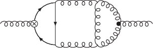
We now consider the diagram shown in Figure 2, which contributes to the massive operator matrix element $A_{Qg}^{(3)}$ , cf. Ref. [16], and derives from the diagram in Figure 1, by adding the local operator insertion $\otimes$ , see [16] and Appendix A, and an external momentum flow $p$ with $p^{2}=0$ . We consider first the case where all exponents of the propagators are equal to one.

Here and in the following we separate a common pre-factor

\displaystyle I_{1a}\equiv\frac{i(\Delta.p)^{N}a_{s}^{3}S_{\varepsilon}^{3}}{(m^{2})^{2-3\frac{\varepsilon}{2}}}\hat{I}_{1a}.

(2.25)

Again the momentum integrals are performed in the order $q,k,l$ through which

	$\displaystyle\hat{I}_{1a}$	$\displaystyle=$	$\displaystyle-\exp\left(-3\frac{\varepsilon}{2}\gamma_{E}\right)\Gamma(2-3\varepsilon/2)\prod_{i=1}^{7}\int_{0}^{1}dw_{i}~\frac{\theta(1-w_{1}-w_{2})w_{1}^{-\varepsilon/2}w_{2}^{-\varepsilon/2}(1-w_{1}-w_{2})}{\displaystyle{\left(1+w_{1}\frac{1-w_{3}}{w_{3}}+w_{2}\frac{1-w_{4}}{w_{4}}\right)^{2-3\varepsilon/2}}}$
			$\displaystyle\times w_{3}^{-1+\varepsilon/2}(1-w_{3})^{\varepsilon/2}w_{4}^{-1+\varepsilon/2}(1-w_{4})^{\varepsilon/2}(1-w_{5}w_{1}-w_{6}w_{2}-(1-w_{1}-w_{2})w_{7})^{N}$

is obtained. The spherical factor $S_{\varepsilon}$ is given by

\displaystyle S_{\varepsilon}=\exp\left[\frac{\varepsilon}{2}\left(\gamma_{E}-\ln(4\pi)\right)\right]~,

(2.27)

and $\gamma_{E}$ the Euler–Mascheroni constant. In the $\overline{\rm MS}$ scheme this factor is later identified by $S_{\varepsilon}\equiv 1$ . It absorbs the universal dependence of $D$ -dimensional integrals on $\ln(4\pi)$ and $\gamma_{E}$ . As in the $2$ –loop case, [28], one observes that the integral–kernel given by the corresponding massive tadpole–integral (2.5) is multiplied by a polynomial containing various integration parameters to the power $N$ . The same holds for the remaining $3$ –loop diagrams. Hence, if a general sum representation for the corresponding tadpole–integrals is known and one knows how to evaluate the corresponding sums, the $3$ –loop massive OMEs can be calculated directly. However, the presence of the polynomial to the power $N$ , which may also involve a finite sum, cf. the Feynman rules given in Appendix 8.1. of Ref. [16], complicates the calculation further, in some cases even in a very essential way.

To perform the remaining integrals for Diagram $I_{1a}$ we split the expression into several finite sums which have a similar structure as $T_{1}$ . One obtains

$\displaystyle\hat{I}_{1a}$	$\displaystyle=$	$\displaystyle\frac{\exp\left(-3\frac{\varepsilon}{2}\gamma_{E}\right)\Gamma(2-3\varepsilon/2)}{(N+1)(N+2)(N+3)}\sum_{m,n=0}^{\infty}\Biggl\{$
		$\displaystyle\hskip 14.22636pt\sum_{t=1}^{N+2}\binom{3+N}{t}\frac{\left(t-\varepsilon/2\right)_{m}\left(2+N+\varepsilon/2\right)_{n+m}\left(3-t+N-\varepsilon/2\right)_{n}}{\left(4+N-\varepsilon\right)_{n+m}}$
		$\displaystyle\hskip 28.45274pt\times\Gamma\left[\begin{array}[]{c}t,t-\varepsilon/2,1+m+\varepsilon/2,1+n+\varepsilon/2,3-t+N,3-t+N-\varepsilon/2\\ 4+N-\varepsilon,1+m,1+n,1+t+m+\varepsilon/2,4-t+n+N+\varepsilon/2\end{array}\right]$
		$\displaystyle\hskip 2.84526pt-\sum_{s=1}^{N+3}\sum_{r=1}^{s-1}\binom{s}{r}\binom{3+N}{s}(-1)^{s}\frac{\left(r-\varepsilon/2\right)_{m}\left(-1+s+\varepsilon/2\right)_{n+m}\left(s-r-\varepsilon/2\right)_{n}}{\left(1+s-\varepsilon\right)_{n+m}}$
		$\displaystyle\hskip 28.45274pt\times\Gamma\left[\begin{array}[]{c}r,r-\varepsilon/2,s-r,1+m+\varepsilon/2,1+n+\varepsilon/2,s-r-\varepsilon/2\\ 1+m,1+n,1+r+m+\varepsilon/2,1+s-r+n+\varepsilon/2,1+s-\varepsilon\end{array}\right]\Biggr\}~.$

After expanding in $\varepsilon$ , the summation can be performed using Sigma and the summation techniques having been explained in [9, 11, 36] before.

The results of the integrals being dealt with in the present paper can be expressed in terms of harmonic sums $S_{\vec{a}}(N)$ [5, 6] and their generalizations $S_{\vec{a}}(\vec{\xi};N)$ [37, 38]. They are defined by :

\displaystyle S_{b,\vec{a}}(N)

\displaystyle=

\displaystyle\sum_{k=1}^{N}\frac{{{\rm sign}(b)}^{k}}{k^{|b|}}S_{\vec{a}}(k),~~~~S_{\emptyset}(k)=1~,

(2.35)

and

\displaystyle S_{b,\vec{a}}(\eta,\vec{\xi};N)

\displaystyle=

\displaystyle\sum_{k=1}^{N}\frac{\eta^{k}}{k^{b}}S_{\vec{a}}(\vec{\xi};k),~~S_{\emptyset}=1,~~~~\eta,\xi\in\mathbb{R},b,a_{i}\in\mathbb{N}\backslash\{0\}~.

(2.36)

In the following we use the short-hand notation for these sums $S_{\vec{a}}(N)\equiv S_{\vec{a}}$ , $S_{\vec{a}}(\vec{\xi};N)\equiv S_{\vec{a}}(\vec{\xi})$ .

Moreover, we calculate the diagrams for all integer values of $N$ , for which they are defined and do not refer either to even or odd moments, as required in subsequent physical applications due to the presence of the respective current crossing relations, cf. [42].

The threefold and fourfold sums in $\hat{I}_{1a}$ yield :

$\displaystyle\hat{I}_{1a}$	$\displaystyle=$	$\displaystyle-\frac{4(N+1){S_{1}}+4}{(N+1)^{2}(N+2)}{\zeta_{3}}+\frac{2{S_{2,1,1}}}{(N+2)(N+3)}+\frac{1}{(N+1)(N+2)(N+3)}\Biggl\{$	(2.37)
		$\displaystyle-2(3N+5){S_{3,1}}-\frac{S_{1}^{4}}{4}+\frac{4(N+1){S_{1}}-4N}{N+1}{S_{2,1}}+2\left[(2N+3){S_{1}}+\frac{5N+6}{N+1}\right]{S_{3}}$
		$\displaystyle+\frac{9+4N}{4}{S_{2}^{2}}+\left[2\frac{7N+11}{(N+1)(N+2)}+\frac{5N}{N+1}{S_{1}}-\frac{5}{2}{S_{1}^{2}}\right]{S_{2}}+\frac{2(3N+5)S_{1}^{2}}{(N+1)(N+2)}$
		$\displaystyle+\frac{N}{N+1}{S_{1}^{3}}+\frac{4(2N+3){S_{1}}}{(N+1)^{2}(N+2)}-\frac{(2N+3){S_{4}}}{2}+8\frac{2N+3}{(N+1)^{3}(N+2)}\Biggr\}$
		$\displaystyle+O(\varepsilon)~,$

which agrees with the fixed moments $N=1\ldots 10$ obtained using ${\sf MATAD}$ [35]. For a direct reference we give a series of moments in Tables 1 and 2 below.

The propagator carrying the operator insertion in Figure 2 also emerges to the second power. The result for the corresponding integral is

$\displaystyle I_{1b}$	$\displaystyle\equiv$	$\displaystyle\frac{i(\Delta.p)^{N}a_{s}^{3}S_{\varepsilon}^{3}}{(m^{2})^{3-3\frac{\varepsilon}{2}}}\hat{I}_{1b}~,$	(2.38)
$\displaystyle\hat{I}_{1b}$	$\displaystyle=$	$\displaystyle\frac{\exp\left(-3\frac{\varepsilon}{2}\gamma_{E}\right)}{(N+1)(N+2)(N+3)}\Gamma\left(3-\frac{3}{2}\varepsilon\right)\Biggl\{-\sum_{m=0}^{\infty}\sum_{n=0}^{\infty}\sum_{l=1}^{N+2}\binom{N+3}{l}$
		$\displaystyle\times B\left(l,m+1+\frac{\varepsilon}{2}\right)B\left(N+3-l,n+1+\frac{\varepsilon}{2}\right)$
		$\displaystyle\times\Gamma\left[\begin{array}[]{c}N+2+\frac{\varepsilon}{2}+m+n\\ m+1,n+1,N+2+\frac{\varepsilon}{2}\end{array}\right]\frac{B\left(l+m-\frac{\varepsilon}{2},N+3-l+n-\frac{\varepsilon}{2}\right)}{(N+4+m+n-\varepsilon)(N+3+m+n-\varepsilon)}$
		$\displaystyle+\frac{1}{N+4}\Biggl[\sum_{m=1}^{\infty}\sum_{n=1}^{\infty}\sum_{l=1}^{N+4}\binom{N+4}{l}\sum_{j=1}^{N+4-l}\binom{N+4-l}{j}(-1)^{j+l}B\left(j,m+1+\frac{\varepsilon}{2}\right)$
		$\displaystyle\times B\left(l,n+1+\frac{\varepsilon}{2}\right)\Gamma\left[\begin{array}[]{c}j+l-2+m+n+\frac{\varepsilon}{2}\\ m+1,n+1,j+l-2+\frac{\varepsilon}{2}\end{array}\right]\frac{B\left(j+m-\frac{\varepsilon}{2},l+n-\frac{\varepsilon}{2}\right)}{j+l+m+n-\varepsilon}$

			$\displaystyle+\sum_{m=1}^{\infty}\sum_{l=1}^{N+4}\binom{N+4}{l}\sum_{j=1}^{N+4-l}\binom{N+4-l}{j}(-1)^{j+l}B\left(j,m+1+\frac{\varepsilon}{2}\right)B\left(l,1+\frac{\varepsilon}{2}\right)$
			$\displaystyle\times\Gamma\left[\begin{array}[]{c}j+l-2+m+\frac{\varepsilon}{2}\\ m+1,j+l-2+\frac{\varepsilon}{2}\end{array}\right]\frac{B\left(j+m-\frac{\varepsilon}{2},l-\frac{\varepsilon}{2}\right)}{j+l+m-\varepsilon}$
			$\displaystyle+\sum_{n=1}^{\infty}\sum_{l=1}^{N+4}\binom{N+4}{l}\sum_{j=1}^{N+4-l}\binom{N+4-l}{j}(-1)^{j+l}B\left(j,1+\frac{\varepsilon}{2}\right)B\left(l,n+1+\frac{\varepsilon}{2}\right)$
			$\displaystyle\times\Gamma\left[\begin{array}[]{c}j+l-2+n+\frac{\varepsilon}{2}\\ n+1,j+l-2+\frac{\varepsilon}{2}\end{array}\right]\frac{B\left(j-\frac{\varepsilon}{2},l+n-\frac{\varepsilon}{2}\right)}{j+l+n-\varepsilon}$
			$\displaystyle+\sum_{l=1}^{N+4}\binom{N+4}{l}\sum_{j=1}^{N+4-l}\binom{N+4-l}{j}(-1)^{j+l}B\left(j,1+\frac{\varepsilon}{2}\right)B\left(l,1+\frac{\varepsilon}{2}\right)\frac{B\left(j-\frac{\varepsilon}{2},l-\frac{\varepsilon}{2}\right)}{j+l-\varepsilon}$
			$\displaystyle-\sum_{m=0}^{\infty}\sum_{n=0}^{\infty}\sum_{l=1}^{N+3}\binom{N+4}{l}B\left(l,m+1+\frac{\varepsilon}{2}\right)B\left(N+4-l,n+1+\frac{\varepsilon}{2}\right)$
			$\displaystyle\times\Gamma\left[\begin{array}[]{c}N+2+m+n+\frac{\varepsilon}{2}\\ m+1,n+1,N+2+\frac{\varepsilon}{2}\end{array}\right]\frac{B\left(l+m-\frac{\varepsilon}{2},N+4-l+n-\frac{\varepsilon}{2}\right)}{N+4+m+n-\varepsilon}\Biggr]\Biggr\}$
		$\displaystyle=$	$\displaystyle\frac{1}{(N+1)(N+2)(N+3)(N+4)}\Biggl\{\frac{1}{2}S_{1}^{4}-\frac{3N+1}{N+1}S_{1}^{3}$
			$\displaystyle-\frac{N^{5}+8N^{4}+45N^{3}+154N^{2}+234N+122}{(N+1)^{2}(N+2)(N+3)}S_{1}^{2}+\frac{4\left(5N^{3}+22N^{2}+23N+3\right)}{(N+1)^{2}(N+2)(N+3)}S_{1}$
			$\displaystyle-\frac{1}{2}\left(2N^{2}+14N+21\right)S_{2}^{2}-\frac{2\left(6N^{5}+46N^{4}+170N^{3}+411N^{2}+575N+324\right)}{(N+1)^{3}(N+2)^{2}(N+3)}$
			$\displaystyle+4(N+3)(N+4)\left[S_{1}+\frac{1}{N+1}\right]\zeta_{3}+\Biggl[5S_{1}^{2}-\frac{5(3N+1)}{(N+1)}S_{1}$

	$\displaystyle-\frac{3N^{5}+28N^{4}+151N^{3}+458N^{2}+638N+318}{(N+1)^{2}(N+2)(N+3)}\Biggr]S_{2}+\Biggl[-\frac{2\left(2N^{3}+16N^{2}+51N+43\right)}{(N+1)}$
	$\displaystyle-4\left(N^{2}+7N+9\right)S_{1}\Biggr]S_{3}+\left(N^{2}+7N+9\right)S_{4}+\Biggl[\frac{2\left(N^{3}+7N^{2}+20N+10\right)}{(N+1)}-8S_{1}\Biggr]S_{2,1}$
	$\displaystyle+2\left(3N^{2}+21N+28\right)S_{3,1}-2\left(N^{2}+7N+8\right)S_{2,1,1}\Biggr\}+O(\varepsilon)~,$		(2.54)

and follows carrying out similar steps as in case of integral $I_{1a}$ . Here,

\displaystyle B(a,b)=\Gamma\left[\begin{array}[]{c}a,b\\ a+b\end{array}\right]

denotes Euler’s Beta-function. The structure of the results of the integrals $I_{1a}$ and $I_{1b}$ are very similar w.r.t. the harmonic sums. However, the polynomial structure in $N$ becomes more involved for $I_{1b}$ .

3 Different Operator Insertions and Fermion Flows

In the following we perform the calculation of ladder-type diagrams of different complexity, which is both due to the number of massive lines and the corresponding local operator insertions. The examples cover the spectrum of possibilities. First we compute diagrams with six massive lines and a second set of examples deals with diagrams which contain three massive lines. The Feynman rules used for the calculation are given in Appendix A.

3.1 Diagrams with Six Fermion Propagators

We consider the diagrams in Figure 3.

In Table 1 we summarize a series of Mellin moments for the diagrams calculated using the code MATAD [35] for comparison to the general- $N$ results.

Diagram $2a$ can be represented in terms of up to sixfold sums.

$\displaystyle I_{2a}$	$\displaystyle\equiv$	$\displaystyle\frac{i(\Delta.p)^{N}a_{s}^{3}S_{\varepsilon}^{3}}{(m^{2})^{2-3\frac{\varepsilon}{2}}}\hat{I}_{2a},$	(3.1)
$\displaystyle\hat{I}_{2a}$	$\displaystyle=$	$\displaystyle\exp\left(-3\frac{\varepsilon}{2}\gamma_{E}\right)\Gamma\left(2-\frac{3}{2}\varepsilon\right)\frac{1}{(N+1)(N+2)}\sum_{m=0}^{\infty}\sum_{n=0}^{\infty}\sum_{l=2}^{N+2}\binom{N+2}{l}\sum_{j=2}^{l}\binom{l}{j}\Biggl\{$	(3.8)
		$\displaystyle\sum_{k=1}^{j}\binom{j}{k}\sum_{r=0}^{l-k}\binom{l-k}{r}(-1)^{l+j+k+r}\;\Gamma\left[\begin{array}[]{c}k+r+m+n+\frac{\varepsilon}{2}\\ m+1,n+1,k+r+\frac{\varepsilon}{2}\end{array}\right]$
		$\displaystyle\times B\left(k,m+1+\frac{\varepsilon}{2}\right)\frac{B\left(k+m-\frac{\varepsilon}{2},r+1+n-\frac{\varepsilon}{2}\right)B\left(r+l-1,n+1+\frac{\varepsilon}{2}\right)}{(k+r+1+m+n-\varepsilon)(N+3-j)}$
		$\displaystyle+\sum_{r=0}^{l-j}\binom{l-j}{r}(-1)^{l+j+r}\;\Gamma\left[\begin{array}[]{c}j+r+m+n+\frac{\varepsilon}{2}\\ m+1,n+1,j+r+\frac{\varepsilon}{2}\end{array}\right]B\left(j,m+1+\frac{\varepsilon}{2}\right)$
		$\displaystyle\times\frac{B\left(j+m-\frac{\varepsilon}{2},r+1+n-\frac{\varepsilon}{2}\right)B\left(r+l-1,n+1+\frac{\varepsilon}{2}\right)}{(j+r+1+m+n-\varepsilon)(N+3-j)}\Biggr\}~.$

Diagram	$N$		Diagram	$N$
$\hat{I}_{1a}$	0	$2-2\zeta_{3}$	$\hat{I}_{2b}$	0	$\frac{1}{8}$
	1	$1-\zeta_{3}$		1	$\frac{5}{108}$
	2	$\frac{199}{324}-\frac{11}{18}\zeta_{3}$		2	$\frac{731}{1728}-\frac{1}{3}\zeta_{3}$
	3	$\frac{91}{216}-\frac{5}{12}\zeta_{3}$		3	$\frac{2142253}{5184000}-\frac{1}{3}\zeta_{3}$
$\hat{I}_{1b}$	0	$-\frac{9}{4}+2\zeta_{3}$	$\hat{I}_{3}$	0	$2-2\zeta_{3}$
	1	$-\frac{247}{216}+\zeta_{3}$		1	$0$
	2	$-\frac{1831}{2592}+\frac{11}{18}\zeta_{3}$		2	$\frac{967}{432}-2\zeta_{3}$
	3	$-\frac{1257637}{2592000}+\frac{5}{12}\zeta_{3}$		3	$0$
$\hat{I}_{2a}$	0	$2-2\zeta_{3}$	$\hat{I}_{4}$	0	$2\zeta_{3}$
	1	$1-\zeta_{3}$		1	$2-2\zeta_{3}$
	2	$\frac{1399}{1296}-\zeta_{3}$		2	$\frac{29}{12}-\frac{83}{36}\zeta_{3}$
	3	$\frac{967}{864}-\zeta_{3}$		3	$\frac{17}{6}-\frac{47}{18}\zeta_{3}$

Table 1: Mellin Moments for the Integrals

\hat{I}_{1a}-\hat{I}_{4}

These sums are performed by Sigma and yield

$\displaystyle\hat{I}_{2a}$	$\displaystyle=$	$\displaystyle\frac{1}{(N+1)(N+2)(N+3)}\Biggl\{2^{N+4}S_{1,2}\left(\frac{1}{2},1\right)+2^{N+3}S_{1,1,1}\left(\frac{1}{2},1,1\right)+\frac{\left(N^{2}+12N+16\right)}{2(N+1)(N+2)}S_{1}^{2}$	(3.9)
		$\displaystyle+\frac{\left(3N^{2}+40N+56\right)}{2(N+1)(N+2)}S_{2}+\frac{1}{6}S_{1}^{3}+\frac{4(2N+3)}{(N+1)^{2}(N+2)}S_{1}-\frac{1}{2}S_{2}S_{1}-(-1)^{N}S_{-3}$
		$\displaystyle+\frac{1}{3}(-3N-17)S_{3}-2(-1)^{N}S_{-2,1}+(-N-3)S_{2,1}-2(-1)^{N}\zeta_{3}-2\left(2^{N+3}-3\right)\zeta_{3}$
		$\displaystyle+\frac{8(2N+3)}{(N+1)^{3}(N+2)}\Biggr\}+O(\varepsilon)~.$

Here generalized harmonic sums emerge with $\xi\in\{\frac{1}{2},1\}$ together with powers $2^{N}$ . In the limit $N\rightarrow\infty$ the generalized harmonic sums approach finite values given below. Still $\hat{I}_{2a}$ does not diverge exponentially due to relations among these special generalized harmonic sums, [38]. The asymptotic series of $\hat{I}_{2a}$ was computed using HarmonicSums [43] and is given by

$\displaystyle\hat{I}_{2a}(N)$	$\displaystyle\simeq$	$\displaystyle\Biggl[\Bigl(\frac{4665}{N^{10}}-\frac{3025}{2N^{9}}+\frac{483}{N^{8}}-\frac{301}{2N^{7}}+\frac{45}{N^{6}}-\frac{25}{2N^{5}}+\frac{3}{N^{4}}-\frac{1}{2N^{3}}\Bigr)L(N)$	(3.10)
		$\displaystyle-\frac{84311831}{168N^{10}}+\frac{73442819}{1008N^{9}}-\frac{495179}{40N^{8}}+\frac{185923}{80N^{7}}-\frac{903}{2N^{6}}+\frac{2029}{24N^{5}}-\frac{55}{4N^{4}}+\frac{3}{2N^{3}}\Biggr]\zeta_{2}$
		$\displaystyle+\Bigl(-\frac{1555}{N^{10}}+\frac{3025}{6N^{9}}-\frac{161}{N^{8}}+\frac{301}{6N^{7}}-\frac{15}{N^{6}}+\frac{25}{6N^{5}}-\frac{1}{N^{4}}+\frac{1}{6N^{3}}\Bigr)L^{3}(N)$
		$\displaystyle+\Bigl(-\frac{15557449}{168N^{10}}+\frac{12331933}{1008N^{9}}-\frac{72181}{40N^{8}}+\frac{22877}{80N^{7}}-\frac{97}{2N^{6}}+\frac{227}{24N^{5}}-\frac{9}{4N^{4}}+\frac{1}{2N^{3}}\Bigr)L^{2}(N)$
		$\displaystyle+\Bigl(\frac{116332471}{240N^{10}}-\frac{3304037}{56N^{9}}+\frac{470549}{60N^{8}}-\frac{1509931}{1440N^{7}}+\frac{2897}{24N^{6}}-\frac{145}{24N^{5}}-\frac{5}{2N^{4}}+\frac{1}{N^{3}}\Bigr)L(N)$
		$\displaystyle-\frac{334237263613}{423360N^{10}}+\frac{1140112957301}{12700800N^{9}}-\frac{158319577}{14400N^{8}}+\frac{1226359}{900N^{7}}-\frac{7771}{48N^{6}}+\frac{1429}{72N^{5}}$
		$\displaystyle-\frac{15}{4N^{4}}+\frac{1}{N^{3}}+\Bigl(-\frac{32633}{N^{10}}+\frac{32545}{3N^{9}}-\frac{3601}{N^{8}}+\frac{3577}{3N^{7}}-\frac{393}{N^{6}}+\frac{385}{3N^{5}}-\frac{41}{N^{4}}$
		$\displaystyle+\frac{37}{3N^{3}}-\frac{3}{N^{2}}\Bigr)\zeta_{3}+O\left(\frac{1}{N^{11}}\right)~,$

where $L(N)=\ln(N)+\gamma_{E}$ . Likewise, one obtains for $I_{2b}$

	$\displaystyle I_{2b}$	$\displaystyle\equiv$	$\displaystyle\frac{i(\Delta.p)^{N}a_{s}^{3}S_{\varepsilon}^{3}}{(m^{2})^{3-3\frac{\varepsilon}{2}}}\hat{I}_{2b},$		(3.11)
	$\displaystyle\hat{I}_{2b}$	$\displaystyle=$	$\displaystyle-\exp\left(-3\frac{\varepsilon}{2}\gamma_{E}\right)\Gamma\left(3-\frac{3}{2}\varepsilon\right)\frac{1}{(N+1)(N+2)}\sum_{m=0}^{\infty}\sum_{n=0}^{\infty}\sum_{l=2}^{N+2}\binom{N+2}{l}\sum_{j=2}^{l}\binom{l}{j}\Biggl[$

	$\displaystyle\phantom{\times}\sum_{k=1}^{j}\binom{j}{k}\sum_{r=0}^{l-k}\binom{l-k}{r}(-1)^{l+j+k+r}\;\Gamma\left[\begin{array}[]{c}k+r+m+n+\frac{\varepsilon}{2}\\ m+1,n+1,k+r+\frac{\varepsilon}{2}\end{array}\right]B\left(k,m+1+\frac{\varepsilon}{2}\right)$
	$\displaystyle\times B(N+3-j,2)\frac{B\left(k+m-\frac{\varepsilon}{2},r+2+n-\frac{\varepsilon}{2}\right)B\left(r+l-1,n+1+\frac{\varepsilon}{2}\right)}{k+r+2+m+n-\varepsilon}$
	$\displaystyle+\sum_{r=0}^{l-j}\binom{l-j}{r}(-1)^{l+j+r}\;\Gamma\left[\begin{array}[]{c}j+r+m+n+\frac{\varepsilon}{2}\\ m+1,n+1,j+r+\frac{\varepsilon}{2}\end{array}\right]B\left(j,m+1+\frac{\varepsilon}{2}\right)$

	$\displaystyle\times B(N+3-j,2)\frac{B\left(j+m-\frac{\varepsilon}{2},r+2+n-\frac{\varepsilon}{2}\right)B\left(r+l-1,n+1+\frac{\varepsilon}{2}\right)}{j+r+2+m+n-\varepsilon}\Biggr\}$	(3.19)
$\displaystyle=$	$\displaystyle\frac{1}{(N+1)(N+2)(N+3)(N+4)}\Biggl\{2^{N+4}NS_{1,2}\left(\frac{1}{2},1\right)+2^{N+3}NS_{1,1,1}\left(\frac{1}{2},1,1\right)$
	$\displaystyle+(-1)^{N}(N^{2}+4N+2)\left(-S_{-3}-2S_{-2,1}-2\zeta_{3}\right)+\frac{1}{3}\left(-6N^{2}-33N-20\right)S_{3}$
	$\displaystyle+\frac{\left(8N^{3}+31N^{2}+17N-18\right)}{2(N+1)(N+2)(N+3)}S_{1}^{2}+\frac{2\left(9N^{3}+43N^{2}+58N+21\right)}{(N+1)^{2}(N+2)(N+3)}S_{1}$
	$\displaystyle+\frac{3\left(12N^{3}+55N^{2}+61N+6\right)}{2(N+1)(N+2)(N+3)}S_{2}-\frac{1}{3}S_{1}^{3}+S_{2}S_{1}+(N+4)S_{2,1}$
	$\displaystyle+2\left(N^{2}-2^{N+3}N+6N+2\right)\zeta_{3}$
	$\displaystyle+\frac{-6N^{5}-14N^{4}+68N^{3}+247N^{2}+225N+36}{(N+1)^{3}(N+2)^{2}(N+3)}\Biggr\}+O(\varepsilon)~.$

Again the sum-structure of the integrals remains the same. Unlike the case for the massless 3-loop Wilson coefficients [22] and massive integrals in [23] the generalized harmonic sums do not vanish diagram by diagram. We remark that sums of this type even emerge in massive 2-loop integrals, if diagrams are simply separated into individual terms in a mathematical manner, e.g. in a fully automated computation to $O(\varepsilon)$ [11], while they are absent in case the diagrams are considered as whole entities being mapped to various final sums [9, 11]. The presence of these generalized harmonic sums does not alter the structure of the diagrams significantly in the special way they appear, as we will outline below.

For diagram 3 a simple representation is obtained :

\displaystyle I_{3}

\displaystyle=

\displaystyle\left[1+(-1)^{N}\right]I_{2a}(N+1)~.

(3.20)

Diagrams with a gluon-quark-quark operator insertion on an external gluon line can always be related to a diagram with the operator insertion on the fermion lines next to this vertex due to the Feynman rule for the operators [16], cf. also Appendix A and [28].

Let us now turn to diagram $I_{4}$ ,

\displaystyle I_{4}

\displaystyle\equiv

\displaystyle\frac{i(\Delta.p)^{N}a_{s}^{3}S_{\varepsilon}^{3}}{(m^{2})^{2-3\frac{\varepsilon}{2}}}\hat{I}_{4}~.

(3.21)

We perform the calculation of this diagram in a different way than used before and apply the $\alpha$ -representation for the Feynman parameters, cf. [44]. The integral is convergent in the limit $\varepsilon\rightarrow 0$ and shall be calculated using the method of hyperlogarithms. This method has been worked out in [34] in case the numerator functions are fixed polynomials, the integrands are rational functions in the parameters $\alpha_{i}$ for convergent integrals in $D=4$ dimensions. It can be applied if an integration order can be found, such that at each integration step the denominator factors into linear polynomials in the respective integration variable.

Integral $\hat{I}_{4}$ is given by :

\displaystyle\hat{I}_{4}

\displaystyle=

\displaystyle\int\cdots\int_{\alpha_{i}>0,\alpha_{1}+\alpha_{2}=1}\prod_{i=1}^{7}d\alpha_{i}\frac{\sum_{j=0}^{N}{T_{4a}^{N-j}T_{4b}^{j}}}{U_{G}^{2}M_{G}^{2}},

(3.22)

with the polynomials, cf. [44],

	$\displaystyle T_{4a}$	$\displaystyle=$	$\displaystyle\alpha_{5}\alpha_{7}\alpha_{4}+\alpha_{2}\alpha_{3}\alpha_{5}+\alpha_{2}\alpha_{5}\alpha_{4}+\alpha_{3}\alpha_{5}\alpha_{7}+\alpha_{2}\alpha_{5}\alpha_{8}+\alpha_{8}\alpha_{5}\alpha_{4}+\alpha_{5}\alpha_{7}\alpha_{8}+\alpha_{2}\alpha_{3}\alpha_{8}$		(3.23)
			$\displaystyle+\alpha_{7}\alpha_{2}\alpha_{8}+\alpha_{6}\alpha_{2}\alpha_{8}+\alpha_{3}\alpha_{7}\alpha_{2}+\alpha_{2}\alpha_{3}\alpha_{6}+\alpha_{4}\alpha_{2}\alpha_{8}+\alpha_{2}\alpha_{6}\alpha_{4}+\alpha_{4}\alpha_{7}\alpha_{2}$		(3.23)

$\displaystyle T_{4b}$	$\displaystyle=$	$\displaystyle\alpha_{2}\alpha_{5}\alpha_{4}+\alpha_{4}\alpha_{2}\alpha_{8}+\alpha_{4}\alpha_{7}\alpha_{2}+\alpha_{2}\alpha_{5}\alpha_{8}+\alpha_{2}\alpha_{3}\alpha_{5}+\alpha_{7}\alpha_{2}\alpha_{8}+\alpha_{3}\alpha_{7}\alpha_{2}+\alpha_{8}\alpha_{5}\alpha_{4}$	(3.24)
		$\displaystyle+\alpha_{5}\alpha_{7}\alpha_{4}+\alpha_{4}\alpha_{1}\alpha_{8}+\alpha_{1}\alpha_{7}\alpha_{4}+\alpha_{3}\alpha_{5}\alpha_{7}+\alpha_{5}\alpha_{7}\alpha_{8}+\alpha_{8}\alpha_{1}\alpha_{7}+\alpha_{1}\alpha_{3}\alpha_{7}$	(3.24)
$\displaystyle U_{G}$	$\displaystyle=$	$\displaystyle\alpha_{2}\alpha_{5}\alpha_{4}+\alpha_{2}\alpha_{3}\alpha_{5}+\alpha_{1}\alpha_{3}\alpha_{5}+\alpha_{5}\alpha_{7}\alpha_{4}+\alpha_{1}\alpha_{6}\alpha_{4}+\alpha_{1}\alpha_{3}\alpha_{6}+\alpha_{2}\alpha_{3}\alpha_{6}+\alpha_{2}\alpha_{6}\alpha_{4}$	(3.25)
		$\displaystyle+\alpha_{5}\alpha_{6}\alpha_{4}+\alpha_{1}\alpha_{5}\alpha_{4}+\alpha_{3}\alpha_{5}\alpha_{7}+\alpha_{1}\alpha_{3}\alpha_{7}+\alpha_{1}\alpha_{7}\alpha_{4}+\alpha_{3}\alpha_{7}\alpha_{2}+\alpha_{4}\alpha_{7}\alpha_{2}+\alpha_{3}\alpha_{5}\alpha_{6}$
		$\displaystyle+\alpha_{2}\alpha_{3}\alpha_{8}+\alpha_{2}\alpha_{5}\alpha_{8}+\alpha_{5}\alpha_{7}\alpha_{8}+\alpha_{8}\alpha_{5}\alpha_{4}+\alpha_{8}\alpha_{5}\alpha_{6}+\alpha_{5}\alpha_{3}\alpha_{8}+\alpha_{1}\alpha_{8}\alpha_{5}+\alpha_{1}\alpha_{8}\alpha_{6}$
		$\displaystyle+\alpha_{6}\alpha_{2}\alpha_{8}+\alpha_{1}\alpha_{8}\alpha_{3}+\alpha_{4}\alpha_{1}\alpha_{8}+\alpha_{4}\alpha_{2}\alpha_{8}+\alpha_{7}\alpha_{2}\alpha_{8}+\alpha_{8}\alpha_{1}\alpha_{7}$
$\displaystyle M_{G}$	$\displaystyle=$	$\displaystyle\alpha_{1}+\alpha_{2}+\alpha_{3}+\alpha_{4}+\alpha_{6}+\alpha_{7}~.$	(3.26)

In order to tackle diagram 4 with the method of hyperlogarithms in case of general values of $N$ , the following ideas have been incorporated. We first perform the transformation

	$\displaystyle\sum_{j=0}^{N}T_{4a}^{N-j}T_{4b}^{j}$	$\displaystyle\rightarrow$	$\displaystyle\sum_{N=0}^{\infty}\sum_{j=0}^{N}x^{N}T_{4a}^{N-j}T_{4b}^{j}=\sum_{N=0}^{\infty}\frac{(T_{4a}x)^{N}-(T_{4b}x)^{N}}{T_{4a}-T_{4b}}$		(3.27)
		$\displaystyle=$	$\displaystyle\frac{1}{T_{4a}-T_{4b}}\left[\frac{1}{1-xT_{4a}}-\frac{1}{1-xT_{4b}}\right]=\frac{x}{(1-xT_{4a})(1-xT_{4b})}~,$		(3.27)

constructing a formal power series being resummed in the tracing parameter $x$ . This effectively moves the action of the local operators into propagator–like terms. For more complicated operator insertions the product structure of the denominator in (3.27) is simply extended. A transformation of this type assumes that one finally can map the function $\tilde{f}(x)$ being obtained back to the desired solution $f(N)$ directly.

We consider the following iterated integrals $\mbox{\rm L}_{\vec{a}}(x)\equiv\mbox{\rm L}_{\vec{a}}$

\displaystyle\mbox{\rm L}_{b,\vec{a}}(x)=\int_{0}^{x}\frac{dy}{y-b}\mbox{\rm L}_{\vec{a}}(y),~~~\mbox{\rm L}_{\emptyset}(y)=1;~~~\mbox{\rm L}_{\underbrace{\mbox{\scriptsize 0, \ldots,0}}_{\mbox{\scriptsize$n$}}}(x)=\frac{1}{n!}\ln^{n}(x)~.

(3.28)

During the integration process the indices $a_{i}$ are usually rational functions of $x$ and the integration variables $\alpha_{i}$ . Because of this the iterated integrals $\mbox{\rm L}_{\vec{a}}$ are called hyperlogarithms rather than polylogarithms over the alphabet $\{a_{1},\ldots,a_{k}\}$ .

$\displaystyle\tilde{I}_{4}(x)$	$\displaystyle=$	$\displaystyle\Biggl[-\frac{1+x}{x^{3}}\mbox{\rm L}_{-1}-\frac{2x-1}{x^{3}}\mbox{\rm L}_{1/2}-\frac{3(1-x)}{x^{3}}\mbox{\rm L}_{1}-\frac{1-2x+x^{2}}{(1-x)x^{3}}\mbox{\rm L}_{0,-1}+\frac{1-2x^{2}}{x^{3}}\mbox{\rm L}_{0,1/2}$
		$\displaystyle-\frac{3-4x-3x^{2}+3x^{3}}{(1-x)x^{3}}\mbox{\rm L}_{0,1}-\frac{1-2x^{2}}{x^{3}}\mbox{\rm L}_{1,1/2}+\frac{(1-x)(2+3x)}{x^{3}}\mbox{\rm L}_{1,1}\Biggr]\zeta_{3}$
		$\displaystyle+\frac{(1+x)}{2x^{3}}\left(3\mbox{\rm L}_{-1,0,0,1}-2\mbox{\rm L}_{-1,0,1,1}-3\mbox{\rm L}_{1,0,0,1}\right)+\frac{1}{x^{2}}\left(6\mbox{\rm L}_{0,0,1,1}-4\mbox{\rm L}_{0,1,0,1}-\mbox{\rm L}_{0,1,1,1}\right)$

	$\displaystyle-\frac{(-1+2x)}{2x^{3}}\left[3\mbox{\rm L}_{1/2,0,0,1}-\mbox{\rm L}_{1/2,0,1,1}-3\mbox{\rm L}_{1/2,1,0,1}+\mbox{\rm L}_{1/2,1,1,1}\right]$
	$\displaystyle-\frac{3}{2x^{2}}\mbox{\rm L}_{1,0,1,1}+\frac{2}{x^{2}}\mbox{\rm L}_{1,1,0,1}-\frac{(-1+x)}{2x^{3}}\mbox{\rm L}_{1,1,1,1}+\frac{2}{x^{2}}\left(\mbox{\rm L}_{0,1,1}-\mbox{\rm L}_{1,0,1}\right)$
	$\displaystyle+\frac{\left(-1+2x+x^{2}\right)}{2(-1+x)x^{3}}\left[3\mbox{\rm L}_{0,-1,0,0,1}-2\mbox{\rm L}_{0,-1,0,1,1}\right]$
	$\displaystyle-\frac{5}{-1+x}\mbox{\rm L}_{0,0,0,1,1}-\frac{5}{2(-1+x)}\mbox{\rm L}_{0,0,1,0,1}+\frac{3(3+x)}{2(-1+x)x}\mbox{\rm L}_{0,0,1,1,1}$
	$\displaystyle-\frac{\left(-1+2x^{2}\right)}{2x^{3}}\left[3\mbox{\rm L}_{0,1/2,0,0,1}+\mbox{\rm L}_{0,1/2,0,1,1}+3\mbox{\rm L}_{0,1/2,1,0,1}-\mbox{\rm L}_{0,1/2,1,1,1}\right]$
	$\displaystyle+\frac{3\left(1-3x^{2}+3x^{3}\right)}{2(-1+x)x^{3}}\mbox{\rm L}_{0,1,0,0,1}+\frac{8-14x+5x^{2}+3x^{3}}{2(-1+x)x^{3}}\mbox{\rm L}_{0,1,0,1,1}$
	$\displaystyle+\frac{8-15x+3x^{2}}{2(-1+x)x^{3}}\mbox{\rm L}_{0,1,1,0,1}-\frac{3(-3+2x)}{2x^{3}}\mbox{\rm L}_{0,1,1,1,1}+\frac{-6+3x+5x^{2}}{x^{3}}\mbox{\rm L}_{1,0,0,1,1}$
	$\displaystyle+\frac{2(-1+x)}{x^{3}}\mbox{\rm L}_{1,1,1,0,1}+\frac{4-2x+5x^{2}}{2x^{3}}\mbox{\rm L}_{1,0,1,0,1}-\frac{-4+6x+3x^{2}}{2x^{3}}\mbox{\rm L}_{1,0,1,1,1}$
	$\displaystyle+\frac{\left(-1+2x^{2}\right)}{2x^{3}}\left[3\mbox{\rm L}_{1,1/2,0,0,1}-\mbox{\rm L}_{1,1/2,0,1,1}\right]-\frac{3(-1+x)(4+3x)}{2x^{3}}\mbox{\rm L}_{1,1,0,0,1}$
	$\displaystyle-\frac{\left(-1+2x^{2}\right)}{2x^{3}}\left[\mbox{\rm L}_{1,1/2,1,0,1}+\mbox{\rm L}_{1,\frac{1}{2},1,1,1}\right]-\frac{(-1+x)(5+3x)}{2x^{3}}\mbox{\rm L}_{1,1,0,1,1}~.$		(3.29)

One first calculates the result of this transformation for integral $\hat{I}_{4}$ in terms of the variable $x$ . It can be expressed in hyperlogarithms $\mbox{\rm L}_{\vec{a}}(x)$ over the alphabet $\{0,1,-1,1/2\}$ ⁶⁶ 6 For more complicated diagrams also the parameter $x$ appears in terms of rational functions in the alphabet. which are thus generalized harmonic polylogarithms [37, 38] : Finally the transformation (3.27) is reversed finding the $N$ th expansion coefficient of (3.29) symbolically using the packages Sigma [32] and HarmonicSums [43]. One obtains in $N$ -space the following representation in terms of harmonic sums and their generalizations :

$\displaystyle\hat{I}_{4}$	$\displaystyle=$	$\displaystyle\frac{P_{1}}{2(1+N)^{5}(2+N)^{5}(3+N)^{5}}+\frac{P_{2}}{(1+N)^{2}(2+N)^{2}(3+N)^{2}}\zeta_{3}$
		$\displaystyle+\frac{(-1)^{N}\left(65+101N+56N^{2}+13N^{3}+N^{4}\right)}{2(1+N)^{2}(2+N)^{2}(3+N)^{2}}S_{-3}+\frac{\left(-24-5N+2N^{2}\right)}{12(2+N)^{2}(3+N)^{2}}S_{1}^{3}$
		$\displaystyle-\frac{1}{2(1+N)(2+N)(3+N)}S_{2}^{2}+\frac{1}{(2+N)(3+N)}S_{1}^{2}S_{2}$
		$\displaystyle+\frac{314+631N+578N^{2}+288N^{3}+68N^{4}+5N^{5}}{4(1+N)^{3}(2+N)^{2}(3+N)^{2}}S_{1}^{2}-\frac{3}{2}S_{5}$
		$\displaystyle-\frac{\left(399+2069N+2774N^{2}+1510N^{3}+349N^{4}+27N^{5}\right)}{6(1+N)^{2}(2+N)^{2}(3+N)^{2}}S_{3}-2S_{-2,-3}$
		$\displaystyle-2\zeta_{3}S_{-2}-S_{-2,1}S_{-2}+\frac{(-1)^{N}\left(65+101N+56N^{2}+13N^{3}+N^{4}\right)}{(1+N)^{2}(2+N)^{2}(3+N)^{2}}S_{-2,1}$
		$\displaystyle+\frac{\left(59+42N+6N^{2}\right)}{2(1+N)(2+N)(3+N)}S_{4}+\frac{(5+N)}{(1+N)(3+N)}\zeta_{3}S_{1}\Bigl(2\Bigr)$
		$\displaystyle-\frac{752+2087N+2490N^{2}+1580N^{3}+558N^{4}+105N^{5}+8N^{6}}{4(1+N)^{3}(2+N)^{2}(3+N)^{2}}S_{2}-\zeta_{3}S_{2}$

	$\displaystyle-\frac{3}{2}S_{3}S_{2}-2S_{2,1}S_{2}+\frac{\left(99+225N+190N^{2}+65N^{3}+7N^{4}\right)}{2(1+N)^{2}(2+N)^{2}(3+N)}S_{2,1}$
	$\displaystyle+\frac{P_{3}}{(1+N)^{4}(2+N)^{4}(3+N)^{4}}S_{1}-\frac{(11+5N)}{(1+N)(2+N)(3+N)}\zeta_{3}S_{1}$
	$\displaystyle-\frac{\left(470+1075N+996N^{2}+447N^{3}+96N^{4}+8N^{5}\right)}{4(1+N)^{2}(2+N)^{2}(3+N)^{2}}S_{2}S_{1}-S_{2,3}$
	$\displaystyle+\frac{(53+29N)}{2(1+N)(2+N)(3+N)}S_{3}S_{1}-\frac{3(3+2N)}{(1+N)(2+N)(3+N)}S_{1}S_{2,1}$
	$\displaystyle+\frac{\left(-79-40N+N^{2}\right)}{2(1+N)(2+N)(3+N)}S_{3,1}-3S_{4,1}+S_{-2,1,-2}$
	$\displaystyle+\frac{2^{1+N}\left(-28-25N-4N^{2}+N^{3}\right)}{(1+N)^{2}(2+N)(3+N)^{2}}S_{1,2}\left(\frac{1}{2},1\right)-\frac{\left(-7+2N^{2}\right)}{(1+N)(2+N)(3+N)}S_{2,1,1}$
	$\displaystyle+5S_{2,2,1}+6S_{3,1,1}+\frac{2^{N}\left(-28-25N-4N^{2}+N^{3}\right)}{(1+N)^{2}(2+N)(3+N)^{2}}S_{1,1,1}\left(\frac{1}{2},1,1\right)$
	$\displaystyle-\frac{(5+N)}{(1+N)(3+N)}S_{1,1,2}\left(2,\frac{1}{2},1\right)-\frac{(5+N)}{2(1+N)(3+N)}S_{1,1,1,1}\left(2,\frac{1}{2},1,1\right)~,$		(3.30)

where

$\displaystyle P_{1}$	$\displaystyle=$	$\displaystyle-31104-159408N-353808N^{2}-446652N^{3}-353808N^{4}-182604N^{5}-61488N^{6}$	(3.31)
		$\displaystyle-13044N^{7}-1584N^{8}-84N^{9},$	(3.31)
$\displaystyle P_{2}$	$\displaystyle=$	$\displaystyle-105+65(-1)^{N}+7\ 2^{4+N}-150N+101(-1)^{N}N+39\ 2^{2+N}N-73N^{2}+56(-1)^{N}N^{2}$	(3.32)
		$\displaystyle+33\ 2^{1+N}N^{2}-12N^{3}+13(-1)^{N}N^{3}+2^{2+N}N^{3}+(-1)^{N}N^{4}-2^{1+N}N^{4},$	(3.32)
$\displaystyle P_{3}$	$\displaystyle=$	$\displaystyle 5436+29004N+67285N^{2}+89175N^{3}+74616N^{4}+41120N^{5}+15107N^{6}+3659N^{7}$	(3.33)
		$\displaystyle+562N^{8}+50N^{9}+2N^{10}~.$	(3.33)

In order to show that the $2^{N}$ -terms are artifacts of the representation as in $I_{2a,b}$ , we calculate the asymptotic representation of $\hat{I}_{4}$ :

$\displaystyle\hat{I}_{4}$	$\displaystyle\simeq$	$\displaystyle\left[\frac{1115231}{20N^{10}}-\frac{74121}{4N^{9}}+\frac{122951}{20N^{8}}-\frac{40677}{20N^{7}}+\frac{13391}{20N^{6}}-\frac{873}{4N^{5}}+\frac{1391}{20N^{4}}-\frac{417}{20N^{3}}+\frac{101}{20N^{2}}\right]\zeta_{2}^{2}$
		$\displaystyle+\Biggl[\left(-\frac{95855}{2N^{10}}+\frac{31525}{2N^{9}}-\frac{10295}{2N^{8}}+\frac{3325}{2N^{7}}-\frac{1055}{2N^{6}}+\frac{325}{2N^{5}}-\frac{95}{2N^{4}}+\frac{25}{2N^{3}}-\frac{5}{2N^{2}}\right)L(N)$
		$\displaystyle-\frac{23280115}{2016N^{10}}+\frac{2093041}{1008N^{9}}-\frac{177251}{1008N^{8}}-\frac{25843}{336N^{7}}+\frac{2569}{48N^{6}}-\frac{155}{8N^{5}}+\frac{91}{24N^{4}}+\frac{2}{3N^{3}}-\frac{11}{12N^{2}}\Biggr]\zeta_{3}$
		$\displaystyle+\Biggl[\left(\frac{19171}{N^{10}}-\frac{6305}{N^{9}}+\frac{2059}{N^{8}}-\frac{665}{N^{7}}+\frac{211}{N^{6}}-\frac{65}{N^{5}}+\frac{19}{N^{4}}-\frac{5}{N^{3}}+\frac{1}{N^{2}}\right)L^{2}(N)$
		$\displaystyle+\left(\frac{103016863}{2520N^{10}}-\frac{3091261}{315N^{9}}+\frac{2571839}{1260N^{8}}-\frac{6215}{21N^{7}}-\frac{293}{20N^{6}}+\frac{2071}{60N^{5}}-\frac{103}{6N^{4}}+\frac{67}{12N^{3}}-\frac{1}{N^{2}}\right)L(N)$
		$\displaystyle+\frac{292993001621}{302400N^{10}}-\frac{4402272031}{30240N^{9}}+\frac{22261739}{840N^{8}}-\frac{78507473}{14112N^{7}}+\frac{180961}{144N^{6}}-\frac{111807}{400N^{5}}+\frac{629}{12N^{4}}$
		$\displaystyle-\frac{319}{72N^{3}}-\frac{7}{4N^{2}}\Biggr]\zeta_{2}$

	$\displaystyle+\left(\frac{249223}{6N^{10}}-\frac{145015}{12N^{9}}+\frac{10295}{3N^{8}}-\frac{11305}{12N^{7}}+\frac{1477}{6N^{6}}-\frac{715}{12N^{5}}+\frac{38}{3N^{4}}-\frac{25}{12N^{3}}+\frac{1}{6N^{2}}\right)L^{3}(N)$
	$\displaystyle+\Bigl(\frac{193493767}{10080N^{10}}+\frac{210658237}{10080N^{9}}-\frac{21541697}{2520N^{8}}+\frac{243269}{96N^{7}}-\frac{30539}{48N^{6}}+\frac{2123}{16N^{5}}-\frac{59}{3N^{4}}$
	$\displaystyle+\frac{5}{8N^{3}}+\frac{1}{2N^{2}}\Bigl)L^{2}(N)$
	$\displaystyle+\Bigl(-\frac{2207364771673}{4233600N^{10}}+\frac{1390655509}{352800N^{9}}+\frac{285594061}{22050N^{8}}-\frac{67234111}{14400N^{7}}+\frac{8617073}{7200N^{6}}-\frac{35209}{144N^{5}}$
	$\displaystyle+\frac{116}{3N^{4}}-\frac{119}{24N^{3}}+\frac{1}{N^{2}}\Bigr)L(N)$
	$\displaystyle+\frac{1344226725047831}{889056000N^{10}}-\frac{165849841805771}{889056000N^{9}}+\frac{808151260279}{27783000N^{8}}-\frac{708430537}{120960N^{7}}+\frac{304474703}{216000N^{6}}$
	$\displaystyle-\frac{606811}{1728N^{5}}+\frac{1867}{24N^{4}}-\frac{1813}{144N^{3}}+\frac{1}{N^{2}}+O\left(\frac{1}{N^{11}}\right)~,$		(3.34)

which shows a convergent behaviour.

In the above expressions generalized harmonic sums occur which are convergent in the limit $N\rightarrow\infty$ . Furthermore, all of them can be represented in terms of multiple zeta values :

$\displaystyle S_{1}\left(\frac{1}{2};\infty\right)$	$\displaystyle=$	$\displaystyle\ln(2)$	(3.35)
$\displaystyle S_{2}\left(\frac{1}{2};\infty\right)$	$\displaystyle=$	$\displaystyle\frac{1}{2}\left[\zeta_{2}-\ln^{2}(2)\right]$	(3.36)
$\displaystyle S_{1,1}\left(\frac{1}{2},1;\infty\right)$	$\displaystyle=$	$\displaystyle\frac{1}{2}\zeta_{2}$	(3.37)
$\displaystyle S_{3}\left(\frac{1}{2};\infty\right)$	$\displaystyle=$	$\displaystyle\frac{1}{6}\ln^{3}(2)-\frac{1}{2}\zeta_{2}\ln(2)+\frac{7}{8}\zeta_{3}$	(3.38)
$\displaystyle S_{1,2}\left(\frac{1}{2},1;\infty\right)$	$\displaystyle=$	$\displaystyle\frac{5}{8}\zeta_{3}$	(3.39)
$\displaystyle S_{2,1}\left(1,\frac{1}{2};\infty\right)$	$\displaystyle=$	$\displaystyle\frac{1}{2}\zeta_{2}\ln(2)+\frac{1}{4}\zeta_{3}+\frac{1}{6}\ln^{3}(2)$	(3.40)
$\displaystyle S_{2,1}\left(\frac{1}{2},1;\infty\right)$	$\displaystyle=$	$\displaystyle\zeta_{3}-\frac{1}{2}\zeta_{2}\ln(2)$	(3.41)
$\displaystyle S_{2,1}\left(\frac{1}{2},2;\infty\right)$	$\displaystyle=$	$\displaystyle\frac{21}{8}\zeta_{3}-\frac{3}{2}\zeta_{2}\ln(2)$	(3.42)
$\displaystyle S_{1,2}\left(\frac{1}{2},2;\infty\right)$	$\displaystyle=$	$\displaystyle\frac{3}{2}\zeta_{2}\ln(2)$	(3.43)
$\displaystyle S_{1,1,1}\left(\frac{1}{2},1,1;\infty\right)$	$\displaystyle=$	$\displaystyle\frac{3\zeta_{3}}{4}$	(3.44)
$\displaystyle S_{1,1,1}\left(\frac{1}{2},2,1;\infty\right)$	$\displaystyle=$	$\displaystyle\frac{3}{2}\ln(2)\zeta_{2}+\frac{7}{4}\zeta_{3}~.$	(3.45)

For completeness, we also give the representations of the generalized harmonic sums in terms of a Mellin transformation

\displaystyle\,\mbox{\bf M}[f(x)](N)=\int_{0}^{1}dxx^{N-1}~f(x),~~\text{resp.}~~\,\mbox{\bf M}\left[\left(\frac{g(x)}{1-x}\right)_{+}\right](N)=\int_{0}^{1}dx\frac{x^{N-1}-1}{1-x}~g(x)~.

(3.46)

It turns out that all cases are related to the usual harmonic polylogarithms over the alphabet $\{-1,0,1\}$ [45], adding in a few cases the letters $1/(\frac{1}{2}-x)$ or $1/(2-x)$ as the first one, for $x\in[0,1]$ . Here the second letter is uncritical. In case of the first letter a new type of $+$ -prescription for the Mellin-transform emerges on $[0,1]$ , through which the singularity of the denominator at $x=1/2$ is regulated,

\displaystyle\,\mbox{\bf M}_{1}\left[\left(\frac{g(x)}{\frac{1}{2}-x}\right)_{+}\right](N)=\int_{0}^{1}dx\frac{(2x)^{N-1}-1}{\frac{1}{2}-x}~g(x)~.

(3.47)

The corresponding Mellin transforms which represent the generalized harmonic sums are :

$\displaystyle S_{1}(2;N)$	$\displaystyle=$	$\displaystyle-\int_{0}^{1}\frac{(2x)^{N}-1}{\frac{1}{2}-x}\,dx$	(3.48)
$\displaystyle S_{1,2}\left(\frac{1}{2},1;N\right)$	$\displaystyle=$	$\displaystyle\frac{5}{8}\zeta_{3}+\int_{0}^{1}\frac{\left(\frac{x}{2}\right)^{N}}{2-x}\mbox{\rm H}_{1,0}(x)\,dx$	(3.49)
$\displaystyle S_{1,1,1}\left(\frac{1}{2},1,1;N\right)$	$\displaystyle=$	$\displaystyle\frac{3}{4}\zeta_{3}-\int_{0}^{1}\frac{\left(\frac{x}{2}\right)^{N}}{2-x}\mbox{\rm H}_{1,1}(x)\,dx$	(3.50)

$\displaystyle S_{1,1,2}\left(2,\frac{1}{2},1;N\right)$	$\displaystyle=$	$\displaystyle-\frac{5}{8}\zeta_{3}\int_{0}^{1}dx\frac{(2x)^{N}-1}{\frac{1}{2}-x}-\int_{0}^{1}\frac{x^{N}-1}{1-x}H_{-1,0,1}(1-x)dx$	(3.51)
		$\displaystyle+\zeta_{2}\int_{0}^{1}dx\frac{x^{N}-1}{1-x}H_{-1}(1-x)$	(3.51)
$\displaystyle S_{1,1,1,1}\left(2,\frac{1}{2},1,1;N\right)$	$\displaystyle=$	$\displaystyle-\frac{3}{4}\zeta_{3}\left[\int_{0}^{1}dx\frac{(2x)^{N}-1}{\frac{1}{2}-x}-\int_{0}^{1}dx\frac{x^{N}-1}{1-x}\right]$	(3.52)
		$\displaystyle-\int_{0}^{1}dx\frac{x^{N}-1}{1-x}\mbox{\rm H}_{2,1,1}(x)~,$	(3.52)

with $\mbox{\rm H}_{-1}(1-x)=\ln(2-x)=-\int_{0}^{x}dy/(2-y)+\ln(2)$ . Similarly, also $\mbox{\rm H}_{-1,0,1}(1-x)$ is a polylogarithm over the alphabet $\{1/x,1/(1-x),1/(2-x)\}$ .

Generalized harmonic sums also occurred in diagram 2. Let us consider the associated functional $\tilde{I}_{2a}$ in similarity to (3.29),

$\displaystyle\tilde{I}_{2a}(x)$	$\displaystyle=$	$\displaystyle\frac{1}{(N+1)(N+2)(N+3)}\Biggl\{-\frac{6x^{3}\zeta_{3}}{(1-x)(1+x)(\frac{1}{2}-x)}+\frac{(-2+x)x^{2}}{(1-x)^{2}}\zeta_{2}\mbox{\rm L}_{1}$	(3.53)
		$\displaystyle+\frac{2(-2+x)x^{2}\left(1-x+x^{2}\right)}{(1-x)^{2}(1+x)(\frac{1}{2}-x)}\mbox{\rm L}_{0,0,1}-\frac{x\left(-4+4x+13x^{2}-17x^{3}+2x^{4}\right)}{2(1-x)^{2}(1+x)(\frac{1}{2}-x)}\mbox{\rm L}_{0,1,1}$
		$\displaystyle+\frac{x\left(5-8x+2x^{2}\right)}{(1-x)(\frac{1}{2}-x)}\mbox{\rm L}_{1,0,1}-\frac{x\left(7-13x+2x^{2}\right)}{2(1-x)(\frac{1}{2}-x)}\mbox{\rm L}_{1,1,1}\Biggr\}~.$

Here all harmonic polylogarithms are formed over the alphabet $\{0,1\}$ and the letter $1/(\frac{1}{2}-x)$ only emerges as pre-factor. It causes the generalized sums in $I_{2a}(N)$ . The structures beyond the usual harmonic polylogarithms in (3.53) are much simpler than in (3.29), which explains the greater difficulty to solve $I_{4}$ using summation technologies.

3.2 Diagrams with Three Fermion Propagators

The corresponding diagrams are given in Figure 4.

Again we first give a number of fixed moments in Table 2. Unlike the former case, the diagrams contain poles up to $1/\varepsilon^{2}$ .

Diagram	N
$\hat{I}_{5a}$	0	$\frac{1}{6}\frac{1}{\varepsilon^{2}}+\frac{1}{9}\frac{1}{\varepsilon}+\frac{13}{54}+\frac{1}{16}\zeta_{2}$
	1	$\frac{1}{12}\frac{1}{\varepsilon^{2}}+\frac{1}{18}\frac{1}{\varepsilon}+\frac{13}{108}+\frac{1}{32}\zeta_{2}$
	2	$\frac{13}{270}\frac{1}{\varepsilon^{2}}+\frac{121}{3600}\frac{1}{\varepsilon}+\frac{138911}{1944000}+\frac{13}{720}\zeta_{2}$
	3	$\frac{11}{360}\frac{1}{\varepsilon^{2}}+\frac{163}{7200}\frac{1}{\varepsilon}+\frac{60911}{1296000}+\frac{11}{960}\zeta_{2}$
$\hat{I}_{5b}$	0	$-\frac{1}{10}\frac{1}{\varepsilon^{2}}+\frac{1}{600}\frac{1}{\varepsilon}-\frac{869}{9000}-\frac{3}{80}\zeta_{2}$
	1	$-\frac{1}{24}\frac{1}{\varepsilon^{2}}+\frac{1}{180}\frac{1}{\varepsilon}-\frac{223}{5400}-\frac{1}{64}\zeta_{2}$
	2	$-\frac{13}{630}\frac{1}{\varepsilon^{2}}+\frac{127}{33075}\frac{1}{\varepsilon}-\frac{2371837}{111132000}-\frac{13}{1680}\zeta_{2}$
	3	$-\frac{11}{960}\frac{1}{\varepsilon^{2}}+\frac{1919}{806400}\frac{1}{\varepsilon}-\frac{8361911}{677376000}-\frac{11}{2560}\zeta_{2}$
$\hat{I}_{6}$	0	$\frac{1}{6}\frac{1}{\varepsilon^{2}}+\frac{1}{9}\frac{1}{\varepsilon}+\frac{13}{54}+\frac{1}{16}\zeta_{2}$
	1	$0$
	2	$\frac{11}{180}\frac{1}{\varepsilon^{2}}+\frac{163}{3600}\frac{1}{\varepsilon}+\frac{60911}{648000}+\frac{11}{480}\zeta_{2}$
	3	$0$
$\hat{I}_{7a}$	0	$\frac{1}{6}\frac{1}{\varepsilon^{2}}+\frac{1}{9}\frac{1}{\varepsilon}+\frac{13}{54}+\frac{1}{16}\zeta_{2}$
	1	$0$
	2	$\frac{1}{54}\frac{1}{\varepsilon^{2}}+\frac{1}{360}\frac{1}{\varepsilon}+\frac{1189}{48600}+\frac{1}{144}\zeta_{2}$
	3	$0$
$\hat{I}_{7b}$	0	$-\frac{2}{15}\frac{1}{\varepsilon^{2}}+\frac{11}{450}\frac{1}{\varepsilon}-\frac{1643}{13500}-\frac{1}{20}\zeta_{2}$
	1	$0$
	2	$-\frac{2}{189}\frac{1}{\varepsilon^{2}}+\frac{19}{2205}\frac{1}{\varepsilon}-\frac{225079}{16669800}-\frac{1}{252}\zeta_{2}$
	3	$0$
$\hat{I}_{8}$	0	$\frac{1}{6}\frac{1}{\varepsilon^{2}}+\frac{1}{9}\frac{1}{\varepsilon}+\frac{13}{54}+\frac{1}{16}\zeta_{2}$
	1	$\frac{1}{12}\frac{1}{\varepsilon^{2}}+\frac{1}{18}\frac{1}{\varepsilon}+\frac{13}{108}+\frac{1}{32}\zeta_{2}$
	2	$\frac{151}{2160}\frac{1}{\varepsilon^{2}}+\frac{1783}{43200}\frac{1}{\varepsilon}+\frac{785701}{7776000}+\frac{151}{5760}\zeta_{2}$
	3	$\frac{31}{720}\frac{1}{\varepsilon^{2}}+\frac{1249}{43200}\frac{1}{\varepsilon}+\frac{166801}{2592000}+\frac{31}{1920}\zeta_{2}$
$\hat{I}_{9a}$	0	$\frac{1}{\varepsilon^{2}}+\frac{3}{2}\frac{1}{\varepsilon}+\frac{13}{4}+\frac{3}{8}\zeta_{2}$
	1	$\frac{3}{4}\frac{1}{\varepsilon^{2}}+\frac{59}{48}\frac{1}{\varepsilon}+\frac{1375}{576}+\frac{9}{32}\zeta_{2}$
	2	$\frac{47}{54}\frac{1}{\varepsilon^{2}}+\frac{73}{54}\frac{1}{\varepsilon}+\frac{2695}{972}+\frac{47}{144}\zeta_{2}$
	3	$\frac{155}{216}\frac{1}{\varepsilon^{2}}+\frac{2035}{1728}\frac{1}{\varepsilon}+\frac{1424773}{622080}+\frac{155}{576}\zeta_{2}$
$\hat{I}_{9b}$	0	$\frac{1}{\varepsilon^{2}}+\frac{3}{2}\frac{1}{\varepsilon}+\frac{13}{4}+\frac{3}{8}\zeta_{2}$
	1	$\frac{1}{2}\frac{1}{\varepsilon^{2}}+\frac{13}{24}\frac{1}{\varepsilon}+\frac{413}{288}+\frac{3}{16}\zeta_{2}$
	2	$\frac{37}{54}\frac{1}{\varepsilon^{2}}+\frac{101}{108}\frac{1}{\varepsilon}+\frac{8333}{3888}+\frac{37}{144}\zeta_{2}$
	3	$\frac{5}{12}\frac{1}{\varepsilon^{2}}+\frac{139}{288}\frac{1}{\varepsilon}+\frac{14297}{11520}+\frac{5}{32}\zeta_{2}$

Table 2: Mellin Moments for Integrals

\hat{I}_{5a}-\hat{I}_{9b}

In a first step the different integrals are represented in finite sums over hypergeometric series keeping the general $\varepsilon$ -dependence. After expanding in $\varepsilon$ , evanescent poles in summation parameters may appear, which have to be dealt with. The resulting indefinite nested sums can again be calculated by SIGMA. For the diagrams $I_{5a}$ and $I_{5b}$ one obtains

$\displaystyle I_{5a(b)}$	$\displaystyle\equiv$	$\displaystyle\frac{i(\Delta.p)^{N}a_{s}^{3}S_{\varepsilon}^{3}}{(m^{2})^{2-3\frac{\varepsilon}{2}}}\hat{I}_{5a(b)}~,$	(3.54)
$\displaystyle\hat{I}_{5a}$	$\displaystyle=$	$\displaystyle\exp\left(-3\frac{\varepsilon}{2}\gamma_{E}\right)\Gamma\left(2-\frac{3}{2}\varepsilon\right)B\left(\frac{\varepsilon}{2},1+\frac{\varepsilon}{2}\right)\sum_{j=0}^{N}\binom{N}{j}\sum_{l=0}^{j}\binom{j}{l}(-1)^{j+l}$	(3.55)
		$\displaystyle\frac{B(-\varepsilon+j+2,3-\varepsilon)}{(l+1)(l+2)(N+1-l)}B\left(\varepsilon-1,-\frac{\varepsilon}{2}+j+3\right)\left[\frac{2}{\varepsilon}+\frac{1}{l+2-\frac{\varepsilon}{2}}+B\left(-\frac{\varepsilon}{2},l+3\right)\right]$
	$\displaystyle=$	$\displaystyle\frac{1}{(N+1)(N+3)(N+4)}\Biggl\{4\left[S_{1}-\frac{N^{2}+N-1}{(N+1)(N+2)}\right]\frac{1}{\varepsilon^{2}}$
		$\displaystyle+\Biggl[\frac{5}{2}S_{1}^{2}-\frac{1}{2}S_{2}+\frac{-5N^{4}-18N^{3}+62N^{2}+289N+244}{(N+1)(N+2)(N+3)(N+4)}S_{1}$
		$\displaystyle+\frac{P_{4}}{(N+1)^{2}(N+2)^{2}(N+3)(N+4)}\Biggr]\frac{1}{\varepsilon}$
		$\displaystyle+\Biggl[\frac{11}{12}S_{1}^{3}+\frac{\left(-8N^{4}+3N^{3}+335N^{2}+994N+736\right)}{4(N+1)(N+2)(N+3)(N+4)}S_{1}^{2}$
		$\displaystyle+\left(\frac{P_{5}}{2(N+1)^{2}(N+2)^{2}(N+3)^{2}(N+4)^{2}}+\frac{11}{4}S_{2}\right)S_{1}$
		$\displaystyle+\frac{P_{6}}{(N+1)^{3}(N+2)^{3}(N+3)^{2}(N+4)^{2}}+\frac{3}{2}\left(S_{1}-\frac{\left(N^{2}+N-1\right)}{(N+1)(N+2)}\right)\zeta_{2}$
		$\displaystyle+\frac{-2N^{4}+9N^{3}+185N^{2}+580N+472}{4(N+1)(N+2)(N+3)(N+4)}S_{2}-\frac{8}{3}S_{3}+6S_{2,1}\Biggr]\Biggr\}+O(\varepsilon),$
$\displaystyle P_{4}$	$\displaystyle=$	$\displaystyle-3N^{6}-65N^{5}-415N^{4}-1109N^{3}-1276N^{2}-468N+64,$	(3.56)
$\displaystyle P_{5}$	$\displaystyle=$	$\displaystyle-12N^{8}-311N^{7}-2943N^{6}-13584N^{5}-32101N^{4}-32407N^{3}+7542N^{2}$	(3.57)
		$\displaystyle+40744N+22784,$	(3.57)
$\displaystyle P_{6}$	$\displaystyle=$	$\displaystyle-24N^{9}-604N^{8}-6089N^{7}-32820N^{6}-104549N^{5}-202546N^{4}$	(3.58)
		$\displaystyle-232976N^{3}-143560N^{2}-32816N+3328,$	(3.58)

$\displaystyle\hat{I}_{5b}$	$\displaystyle=$	$\displaystyle\exp\left(-3\frac{\varepsilon}{2}\gamma_{E}\right)\Gamma\left(3-\frac{3}{2}\varepsilon\right)\sum_{l=0}^{N}\binom{N}{l}\sum_{j=0}^{l}\binom{l}{j}\frac{(-1)^{j+l}}{(j+1)(j+2)}B\left(\frac{\varepsilon}{2},1+\frac{\varepsilon}{2}\right)$	(3.59)
		$\displaystyle\times B(N+1-j,2)B(l+2-\varepsilon,4-\varepsilon)$
		$\displaystyle\times B\left(\varepsilon-1,l+3-\frac{\varepsilon}{2}\right)\left[-\frac{2}{\varepsilon}-B\left(-\frac{\varepsilon}{2},j+3\right)-\frac{1}{j+2-\frac{\varepsilon}{2}}\right]$
	$\displaystyle=$	$\displaystyle\frac{1}{(N+1)(N+3)(N+4)(N+5)}\Biggl\{12\Biggl[\frac{\left(N^{2}+N-1\right)}{(N+1)(N+2)}-S_{1}\Biggr]\frac{1}{\varepsilon^{2}}$
		$\displaystyle+\Biggl[-6S_{1}^{2}+\frac{\left(25N^{5}+261N^{4}+775N^{3}+3N^{2}-2744N-2496\right)}{(N+1)(N+2)(N+3)(N+4)(N+5)}S_{1}$
		$\displaystyle+\frac{-N^{7}+104N^{6}+1497N^{5}+7703N^{4}+18378N^{3}+20465N^{2}+8566N+24}{(N+1)^{2}(N+2)^{2}(N+3)(N+4)(N+5)}\Biggr]\frac{1}{\varepsilon}$
		$\displaystyle+\Biggl[-2S_{1}^{3}+\frac{\left(10N^{5}+87N^{4}+97N^{3}-915N^{2}-2699N-1908\right)}{(N+1)(N+2)(N+3)(N+4)(N+5)}S_{1}^{2}$

		$\displaystyle+\left[\frac{P_{7}}{2(N+1)^{2}(N+2)^{2}(N+3)^{2}(N+4)^{2}(N+5)^{2}}-12S_{2}\right]S_{1}$
		$\displaystyle+\frac{P_{8}}{2(N+1)^{3}(N+2)^{3}(N+3)^{2}(N+4)^{2}(N+5)^{2}}$
		$\displaystyle+\frac{9}{2}\left[\frac{\left(N^{2}+N-1\right)}{(N+1)(N+2)}-S_{1}\right]\zeta_{2}+\frac{\left(11N^{2}-39N-74\right)}{2(N+1)(N+2)}S_{2}+5S_{3}-12S_{2,1}\Biggr]\Biggr\}+O(\varepsilon),$
$\displaystyle P_{7}$	$\displaystyle=$	$\displaystyle 5N^{10}+605N^{9}+12811N^{8}+124145N^{7}+674565N^{6}+2189463N^{5}+4196977N^{4}$	(3.61)
		$\displaystyle+4214683N^{3}+1030490N^{2}-1666304N-1086816,$	(3.61)
$\displaystyle P_{8}$	$\displaystyle=$	$\displaystyle-15N^{12}-497N^{11}-5910N^{10}-27570N^{9}+35363N^{8}+1069961N^{7}+5838492N^{6}$	(3.62)
		$\displaystyle+17154824N^{5}+30447858N^{4}+32466210N^{3}+18880180N^{2}$
		$\displaystyle+4223536N-333696.$

Again both results show a similar structure.

Integral $I_{6}$ is related to $I_{5a}$ by

\displaystyle I_{6}(N)=\left[1+(-1)^{N}\right]I_{5a}(N+1)~.

(3.63)

For the diagram $7_{a,b}$ an all- $\varepsilon$ representation without any sums may be obtained. As a result only single harmonic sums occur after expanding in $\varepsilon$ .

$\displaystyle I_{7a(b)}$	$\displaystyle\equiv$	$\displaystyle\frac{i(\Delta.p)^{N}a_{s}^{3}S_{\varepsilon}^{3}}{(m^{2})^{2-3\frac{\varepsilon}{2}}}\hat{I}_{7a(b)},$	(3.64)
$\displaystyle\hat{I}_{7a}$	$\displaystyle=$	$\displaystyle-\exp\left(-3\frac{\varepsilon}{2}\gamma_{E}\right)\Gamma\left(2-\frac{3\varepsilon}{2}\right)B\left(\frac{\varepsilon}{2},\frac{\varepsilon}{2}+1\right)\frac{[1+(-1)^{N}]}{(N+1)(N+2)(N+3)}$
		$\displaystyle\Biggl\{-\frac{2}{\varepsilon}-\frac{1}{N+3-\frac{\varepsilon}{2}}-B\left(-\frac{\varepsilon}{2},N+4\right)\Biggr\}$
		$\displaystyle\Gamma\left[\begin{array}[]{c}-1+\varepsilon,3+N-\varepsilon,2-\varepsilon,N+3-\frac{\varepsilon}{2}\\ N+2+\frac{\varepsilon}{2},N+5-2\varepsilon\end{array}\right]$

$\displaystyle=$	$\displaystyle\frac{\left[1+(-1)^{N}\right]}{(N+1)(N+3)^{2}(N+4)}\Biggl\{2\left[S_{1}+\frac{2N+3}{(N+1)(N+2)}\right]\frac{1}{\varepsilon^{2}}$	(3.68)
	$\displaystyle+\Biggl[\frac{1}{2}\left[S_{1}^{2}+S_{2}\right]-{\frac{(3\,{N}^{4}+18\,{N}^{3}+21\,{N}^{2}-28\,N-40)}{(N+4)(N+3)(N+2)(N+1)}}S_{1}$
	$\displaystyle-2\,\frac{3\,{N}^{5}+23\,{N}^{4}+53\,{N}^{3}+21\,{N}^{2}-57\,N-48}{(N+1)^{2}(N+2)^{2}(N+3)(N+4)}\Biggr]\frac{1}{\varepsilon}$
	$\displaystyle+\Biggl[\frac{1}{12}S_{1}^{3}+\frac{1}{6}S_{3}+{\frac{13}{4}}S_{1}S_{2}-\frac{1}{4}\frac{(3\,{N}^{4}-6\,{N}^{3}-183\,{N}^{2}-568\,N-472)}{(N+1)(N+2)(N+3)(N+4)}S_{2}$
	$\displaystyle-\frac{(3\,{N}^{4}+18\,{N}^{3}+21\,{N}^{2}-28\,N-40)}{4(N+1)(N+2)(N+3)(N+4)}S_{1}^{2}+\frac{3}{4}\left[S_{1}+\frac{(2\,N+3)}{(N+1)(N+2)}\right]\zeta_{2}$
	$\displaystyle-\frac{P_{9}}{2(N+1)^{2}(N+2)^{2}(N+3)^{2}(N+4)^{2}}S_{1}$
	$\displaystyle-\frac{P_{10}}{2(N+3)^{2}(N+4)^{2}(N+1)^{3}(N+2)^{3}}\Biggr]\Biggr\}+O(\varepsilon)~,$

$\displaystyle P_{9}$	$\displaystyle=$	$\displaystyle 36\,{N}^{7}+511\,{N}^{6}+2878\,{N}^{5}+8037\,{N}^{4}+10942\,{N}^{3}+4576\,{N}^{2}$	(3.69)
		$\displaystyle-4128\,N-3648~,$	(3.69)
$\displaystyle P_{10}$	$\displaystyle=$	$\displaystyle 69\,{N}^{8}+1082\,{N}^{7}+6983\,{N}^{6}+23746\,{N}^{5}+44608\,{N}^{4}+41876\,{N}^{3}+7768\,{N}^{2}$	(3.70)
		$\displaystyle-17008\,N-9984~,$	(3.70)
$\displaystyle\hat{I}_{7b}$	$\displaystyle=$	$\displaystyle\exp\left(-3\frac{\varepsilon}{2}\gamma_{E}\right)\frac{(1+(-1)^{N})}{(N+1)(N+2)(N+3)}\Gamma\left(3-\frac{3}{2}\varepsilon\right)B\left(3-\varepsilon,N+3-\varepsilon\right)$
		$\displaystyle\times B\left(\frac{\varepsilon}{2},1+\frac{\varepsilon}{2}\right)B\left(\varepsilon-1,N+3-\frac{\varepsilon}{2}\right)\left[-B\left(-\frac{\varepsilon}{2},N+4\right)-\frac{1}{N+3-\frac{\varepsilon}{2}}-\frac{2}{\varepsilon}\right]$
	$\displaystyle=$	$\displaystyle\frac{[1+(-1)^{N}]}{(N+1)(N+3)^{2}(N+4)(N+5)}\Biggl\{-8\Biggl[S_{1}+\frac{\left(3+2\,N\right)}{(N+1)(N+2)}\Biggr]\frac{1}{\varepsilon^{2}}$
		$\displaystyle+2\Biggl[-\left(S_{1}^{2}+S_{2}\right)+\frac{11\,{N}^{5}+133\,{N}^{4}+567\,{N}^{3}+999\,{N}^{2}+610\,N+8}{(N+1)(N+2)(N+3)(N+4)(N+5)}S_{1}$
		$\displaystyle+\frac{22\,{N}^{6}+301\,{N}^{5}+1563\,{N}^{4}+3869\,{N}^{3}+4667\,{N}^{2}+2394\,N+264}{(N+1)^{2}(N+2)^{2}(N+3)(N+4)(N+5)}\Biggr]\frac{1}{\varepsilon}$
		$\displaystyle+\Biggl[-\frac{2}{3}S_{3}-\frac{1}{3}S_{1}^{3}-13S_{1}S_{2}-3S_{1}\zeta_{2}-3\,\frac{\left(3+2\,N\right)}{(N+1)(N+2)}\zeta_{2}$
		$\displaystyle+\frac{11\,{N}^{5}+133\,{N}^{4}+567\,{N}^{3}+999\,{N}^{2}+610\,N+8}{2(N+1)(N+2)(N+3)(N+4)(N+5)}S_{1}^{2}\Biggr]$
		$\displaystyle+\frac{11\,{N}^{5}+85\,{N}^{4}-81\,{N}^{3}-2121\,{N}^{2}-5654\,N-4312}{2(N+1)(N+2)(N+3)(N+4)(N+5)}S_{2}$
		$\displaystyle-2\,\frac{P_{11}}{(N+1)^{2}(N+2)^{2}(N+3)^{2}(N+4)^{2}(N+5)^{2}}S_{1}$

		$\displaystyle-\frac{P_{12}}{(N+1)^{3}(N+2)^{3}(N+3)^{2}(N+4)^{2}(N+5)^{2}}\Biggr\}+O(\varepsilon),$	(3.71)
$\displaystyle P_{11}$	$\displaystyle=$	$\displaystyle 9\,{N}^{10}+182\,{N}^{9}+1388\,{N}^{8}+4103\,{N}^{7}-4913\,{N}^{6}-72860\,{N}^{5}-225446\,{N}^{4}$	(3.72)
		$\displaystyle-327313\,{N}^{3}-198070\,{N}^{2}+17240\,N+52416,$	(3.72)
$\displaystyle P_{12}$	$\displaystyle=$	$\displaystyle 36\,{N}^{11}+793\,{N}^{10}+6942\,{N}^{9}+28237\,{N}^{8}+28250\,{N}^{7}-224189\,{N}^{6}$	(3.73)
		$\displaystyle-1079534\,{N}^{5}-2213865\,{N}^{4}-2276462\,{N}^{3}-830640\,{N}^{2}$
		$\displaystyle+388496\,N+315456.$

Diagram 8, despite being expressed only by a threefold sum, is more demanding. One obtains

$\displaystyle I_{8}$	$\displaystyle\equiv$	$\displaystyle\frac{i(\Delta.p)^{N}a_{s}^{3}S_{\varepsilon}^{3}}{(m^{2})^{2-3\frac{\varepsilon}{2}}}\hat{I}_{8},$	(3.74)
$\displaystyle\hat{I}_{8}$	$\displaystyle=$	$\displaystyle-\exp\left(-3\frac{\varepsilon}{2}\gamma_{E}\right)\Gamma(\varepsilon-1)\Gamma\left(2-\frac{3}{2}\varepsilon\right)B\left(\frac{\varepsilon}{2},1+\frac{\varepsilon}{2}\right)\sum_{i=0}^{N}\sum_{j=0}^{N-i}\binom{N-i}{j}(-1)^{j}$	(3.78)
		$\displaystyle\times\sum_{l=0}^{i+j}\binom{i+j}{l}(-1)^{l}\Gamma\left[\begin{array}[]{c}3+j+i-\frac{\varepsilon}{2},3+i-\varepsilon,2+j-\varepsilon\\ 5+i+j-2\varepsilon,2+i+j+\frac{\varepsilon}{2}\end{array}\right]$
		$\displaystyle\times\frac{1}{(l+1)(l+2)(N+1-l)}\left[B\left(-\frac{\varepsilon}{2},1\right)-B\left(l+2-\frac{\varepsilon}{2},1\right)-B\left(-\frac{\varepsilon}{2},l+3\right)\right]$
	$\displaystyle=$	$\displaystyle\frac{1}{(N+2)(N+4)(N+5)}\Biggl\{\Biggl[\Biggl(\frac{2(-1)^{N}\left(N^{2}+5N+7\right)}{(N+2)(N+3)^{2}}$
		$\displaystyle+\frac{2\left(2N^{3}+13N^{2}+27N+20\right)}{(N+1)(N+3)^{2}}\Biggr)S_{1}+S_{1}^{2}+3S_{2}+\frac{2(-1)^{N}(2N^{3}+13N^{2}+29N+21)}{(N+1)(N+2)^{2}(N+3)^{2}}$
		$\displaystyle-\frac{2\left(2N^{6}+18N^{5}+57N^{4}+60N^{3}-53N^{2}-163N-99\right)}{(N+1)^{2}(N+2)^{2}(N+3)^{2}}\Biggr]\frac{1}{\varepsilon^{2}}$
		$\displaystyle+\frac{1}{N+3}\Biggl[\frac{1}{2}(N+3)S_{1}^{3}+\Biggl(\frac{(-1)^{N}\left(N^{2}+5N+7\right)}{2(N+2)(N+3)}$
		$\displaystyle+\frac{2N^{6}+43N^{5}+360N^{4}+1529N^{3}+3524N^{2}+4218N+2048}{2(N+1)(N+2)(N+3)(N+4)(N+5)}\Biggr)S_{1}^{2}$
		$\displaystyle+\Biggl(\frac{P_{13}}{(N+1)^{2}(N+2)(N+3)^{2}(N+4)(N+5)}$
		$\displaystyle+\frac{(-1)^{N}P_{14}}{(N+1)^{2}(N+2)^{2}(N+3)^{2}(N+4)(N+5)}$
		$\displaystyle+4S_{-2}\Biggr)S_{1}+\Biggl(\frac{7}{2}(N+3)S_{1}+\frac{(-1)^{N}\left(N^{2}+5N+7\right)}{2(N+2)(N+3)}$
		$\displaystyle+\frac{-10N^{6}-133N^{5}-612N^{4}-915N^{3}+1052N^{2}+4246N+3104}{2(N+1)(N+2)(N+3)(N+4)(N+5)}\Biggr)S_{2}$
		$\displaystyle+\frac{4(2N+3)}{(N+1)(N+2)}S_{-2}+2(N+5)S_{3}-4(N+3)S_{2,1}$

	$\displaystyle+\frac{(-1)^{N}P_{15}}{(N+1)^{3}(N+2)^{3}(N+3)^{2}(N+4)(N+5)}$
	$\displaystyle+\frac{P_{16}}{(N+1)^{3}(N+2)^{3}(N+3)^{2}(N+4)(N+5)}\Biggr]\frac{1}{\varepsilon}$
	$\displaystyle+\frac{1}{N+3}\Biggl[\frac{7}{48}(N+3)S_{1}^{4}+\Biggl(\frac{(-1)^{N}\left(N^{2}+5N+7\right)}{12(N+2)(N+3)}$
	$\displaystyle+\frac{2N^{6}+59N^{5}+588N^{4}+2805N^{3}+7040N^{2}+8974N+4544}{12(N+1)(N+2)(N+3)(N+4)(N+5)}\Biggr)S_{1}^{3}$
	$\displaystyle+\Biggl(\frac{(-1)^{N}P_{17}}{4(N+1)^{2}(N+2)^{2}(N+3)^{2}(N+4)(N+5)}$
	$\displaystyle+\frac{P_{18}}{4(N+1)^{2}(N+2)^{2}(N+3)^{2}(N+4)^{2}(N+5)^{2}}+7S_{-2}\Biggr)S_{1}^{2}$
	$\displaystyle+\Biggl(\frac{(-1)^{N}P_{19}}{2(N+1)^{3}(N+2)^{3}(N+3)^{3}(N+4)^{2}(N+5)^{2}}$
	$\displaystyle+\frac{P_{20}}{2(N+1)^{3}(N+2)^{2}(N+3)^{3}(N+4)^{2}(N+5)^{2}}+5S_{-3}$
	$\displaystyle-\frac{2\left(5N^{5}+49N^{4}+104N^{3}-285N^{2}-1213N-1036\right)S_{-2}}{(N+1)(N+2)(N+3)(N+4)(N+5)}\Biggr)S_{1}+\frac{(55N+141)}{16}S_{2}^{2}$
	$\displaystyle+\frac{(-1)^{N}P_{21}}{2(N+1)^{4}(N+2)^{4}(N+3)^{3}(N+4)^{2}(N+5)^{2}}$
	$\displaystyle+\frac{P_{22}}{2(N+1)^{4}(N+2)^{4}(N+3)^{3}(N+4)^{2}(N+5)^{2}}+\frac{5(2N+3)}{(N+1)(N+2)}S_{-3}$
	$\displaystyle-\frac{4\left(5N^{6}+63N^{5}+275N^{4}+425N^{3}-160N^{2}-1004N-684\right)S_{-2}}{(N+1)^{2}(N+2)^{2}(N+3)(N+4)(N+5)}$
	$\displaystyle+\Biggl(\frac{3(9N+31)}{8}S_{1}^{2}+\Biggl(\frac{13(-1)^{N}\left(N^{2}+5N+7\right)}{4(N+2)(N+3)}$
	$\displaystyle+\frac{-10N^{6}-65N^{5}+420N^{4}+5213N^{3}+18860N^{2}+29514N+16976}{4(N+1)(N+2)(N+3)(N+4)(N+5)}\Biggr)S_{1}$
	$\displaystyle+\frac{(-1)^{N}P_{23}}{4(N+1)^{2}(N+2)^{2}(N+3)^{2}(N+4)(N+5)}$
	$\displaystyle+\frac{P_{24}}{4(N+1)^{2}(N+2)^{2}(N+3)^{2}(N+4)^{2}(N+5)^{2}}+S_{-2}\Biggr)S_{2}+\zeta_{2}\Biggl(\frac{3}{8}(N+3)S_{1}^{2}$
	$\displaystyle+\Biggl(\frac{3(-1)^{N}\left(N^{2}+5N+7\right)}{4(N+2)(N+3)}+\frac{3\left(2N^{3}+13N^{2}+27N+20\right)}{4(N+1)(N+3)}\Biggr)S_{1}$
	$\displaystyle-\frac{3\left(2N^{6}+18N^{5}+57N^{4}+60N^{3}-53N^{2}-163N-99\right)}{4(N+1)^{2}(N+2)^{2}(N+3)}$
	$\displaystyle+\frac{3(-1)^{N}\left(2N^{3}+13N^{2}+29N+21\right)}{4(N+1)(N+2)^{2}(N+3)}+\frac{9}{8}(N+3)S_{2}\Biggr)+\Biggl(\frac{(-1)^{N}\left(N^{2}+5N+7\right)}{6(N+2)(N+3)}$

		$\displaystyle+\frac{-34N^{5}-383N^{4}-1379N^{3}-1280N^{2}+1830N+2632}{6(N+1)(N+2)(N+3)(N+4)}+\frac{(13N+105)}{6}S_{1}\Biggr)S_{3}$	(3.79)
		$\displaystyle+\frac{(53-N)}{8}S_{4}+\left(-\frac{6(2N+3)}{(N+1)(N+2)}-6S_{1}\right)S_{-2,1}$
		$\displaystyle+\left(\frac{12N^{5}+140N^{4}+546N^{3}+725N^{2}-93N-532}{(N+1)(N+2)(N+4)(N+5)}+(-4N-15)S_{1}\right)S_{2,1}$
		$\displaystyle+(N-11)S_{3,1}+(N+9)S_{2,1,1}\Biggr]\Biggr\}+O(\varepsilon)~,$
$\displaystyle P_{13}$	$\displaystyle=$	$\displaystyle-5N^{8}-68N^{7}-264N^{6}+410N^{5}+6293N^{4}+20720N^{3}+32900N^{2}$	(3.80)
		$\displaystyle+26206N+8440,$	(3.80)
$\displaystyle P_{14}$	$\displaystyle=$	$\displaystyle-3N^{8}-49N^{7}-321N^{6}-1069N^{5}-1863N^{4}-1559N^{3}-773N^{2}$	(3.81)
		$\displaystyle-1199N-1108,$	(3.81)
$\displaystyle P_{15}$	$\displaystyle=$	$\displaystyle-6N^{9}-108N^{8}-810N^{7}-3288N^{6}-7855N^{5}-11456N^{4}-11282N^{3}$	(3.82)
		$\displaystyle-10300N^{2}-9171N-4164,$	(3.82)
$\displaystyle P_{16}$	$\displaystyle=$	$\displaystyle-3N^{11}-112N^{10}-1610N^{9}-12443N^{8}-58690N^{7}-178509N^{6}-355289N^{5}$	(3.83)
		$\displaystyle-451853N^{4}-334491N^{3}-98371N^{2}+31775N+23364,$	(3.83)
$\displaystyle P_{17}$	$\displaystyle=$	$\displaystyle-3N^{8}-49N^{7}-321N^{6}-1069N^{5}-1863N^{4}-1559N^{3}-773N^{2}$	(3.84)
		$\displaystyle-1199N-1108,$	(3.84)
$\displaystyle P_{18}$	$\displaystyle=$	$\displaystyle-8N^{11}-189N^{10}-1643N^{9}-4234N^{8}+32416N^{7}+340621N^{6}+1490447N^{5}$	(3.85)
		$\displaystyle+3864842N^{4}+6329756N^{3}+6460920N^{2}+3775088N+971008,$	(3.85)
$\displaystyle P_{19}$	$\displaystyle=$	$\displaystyle-42N^{12}-1213N^{11}-15525N^{10}-115864N^{9}-557609N^{8}-1804421N^{7}-3966084N^{6}$	(3.86)
		$\displaystyle-5845058N^{5}-5625111N^{4}-3597908N^{3}-2035597N^{2}-1373344N-553968,$	(3.86)
$\displaystyle P_{20}$	$\displaystyle=$	$\displaystyle-12N^{13}-523N^{12}-9558N^{11}-98647N^{10}-644321N^{9}-2799010N^{8}-8183392N^{7}$	(3.87)
		$\displaystyle-15639871N^{6}-17214281N^{5}-4125073N^{4}+17049900N^{3}+25968164N^{2}$
		$\displaystyle+16422416N+4131840,$
$\displaystyle P_{21}$	$\displaystyle=$	$\displaystyle-81N^{13}-2458N^{12}-33378N^{11}-267579N^{10}-1405780N^{9}-5075289N^{8}$	(3.88)
		$\displaystyle-12828559N^{7}-22692458N^{6}-27711081N^{5}-23127963N^{4}-14102081N^{3}$
		$\displaystyle-8182893N^{2}-4780496N-1528944,$
$\displaystyle P_{22}$	$\displaystyle=$	$\displaystyle-60N^{15}-2640N^{14}-51484N^{13}-594504N^{12}-4564031N^{11}-24724313N^{10}$	(3.89)
		$\displaystyle-97683496N^{9}-286337829N^{8}-626024531N^{7}-1014709686N^{6}-1194939874N^{5}$
		$\displaystyle-978463105N^{4}-504961532N^{3}-120080691N^{2}+14776800N+11512944,$
$\displaystyle P_{23}$	$\displaystyle=$	$\displaystyle-3N^{8}-25N^{7}+147N^{6}+2723N^{5}+14685N^{4}+40381N^{3}+60691N^{2}$	(3.90)
		$\displaystyle+46645N+14012,$	(3.90)
$\displaystyle P_{24}$	$\displaystyle=$	$\displaystyle-2N^{11}-177N^{10}-3713N^{9}-36850N^{8}-204686N^{7}-647555N^{6}-952035N^{5}$	(3.91)
		$\displaystyle+618266N^{4}+5332620N^{3}+9769044N^{2}+8340336N+2862784.$	(3.91)

The contributions to diagram $9a$ are derived via sixfold nested sums:

\displaystyle I_{9a/b}

\displaystyle\equiv

\displaystyle\frac{i(\Delta.p)^{N}a_{s}^{3}S_{\varepsilon}^{3}}{(m^{2})^{1-3\frac{\varepsilon}{2}}}\hat{I}_{9a/b},

(3.92)

$\displaystyle\hat{I}_{9a}$	$\displaystyle=$	$\displaystyle\exp\left(-3\frac{\varepsilon}{2}\gamma_{E}\right)\Gamma\left(1-3\frac{\varepsilon}{2}\right)\sum_{j=0}^{N}\binom{N+2}{j+2}\sum_{k=0}^{j}\binom{j+1}{k+1}\sum_{l=0}^{k}\binom{k}{l}(-1)^{k+l}$
		$\displaystyle\sum_{q=0}^{N-j}\binom{N-j}{q}(-1)^{N-j-q}\sum_{r_{2}=0}^{N-l-q}\binom{N-l-q}{r_{2}}$
		$\displaystyle\sum_{r_{1}=0}^{N-l-q-r_{2}}\binom{N-l-q-r_{2}}{r_{1}}\frac{B(1-\varepsilon,N+2-j-\varepsilon)B(\frac{\varepsilon}{2},k+1+\frac{\varepsilon}{2})}{(N+1-q-r_{1}-r_{2})(q+r_{2}+1)}$
		$\displaystyle B(r_{2}+\varepsilon,r_{1}+1)B\left(N+1-l-q-r_{1}-r_{2}-\frac{\varepsilon}{2},r_{1}+r_{2}+1+\varepsilon\right)$
	$\displaystyle=$	$\displaystyle\frac{1}{(N+3)(N+4)}\Biggl\{\Biggl[-\frac{4\left(N^{3}+3N^{2}-N-5\right)}{(N+1)(N+2)(N+3)}S_{1}+2S_{1}^{2}+\frac{4(-1)^{N}}{N+3}S_{1}+4S_{-2}$
		$\displaystyle+2(2N+5)S_{2}+\frac{4(-1)^{N}\left(2N^{3}+7N^{2}+4N-3\right)}{(N+1)^{2}(N+2)^{2}(N+3)}+\frac{4\left(6N^{3}+34N^{2}+63N+39\right)}{(N+1)^{2}(N+2)^{2}(N+3)}\Biggr]\frac{1}{\varepsilon^{2}}$
		$\displaystyle+\Biggl[\frac{\left(-4N^{4}-25N^{3}-30N^{2}+49N+76\right)}{(N+1)(N+2)(N+3)(N+4)}S_{1}^{2}-\frac{4\left(2N^{4}+14N^{3}+27N^{2}+5N-16\right)}{(N+1)(N+2)(N+3)(N+4)}S_{-2}$
		$\displaystyle+\frac{\left(10N^{4}+73N^{3}+158N^{2}+73N-52\right)}{(N+1)(N+2)(N+3)(N+4)}S_{2}$
		$\displaystyle+\frac{2(-1)^{N}\left(12N^{5}+127N^{4}+538N^{3}+1177N^{2}+1354N+648\right)}{(N+1)^{2}(N+2)^{2}(N+3)^{2}(N+4)}S_{1}$
		$\displaystyle-\frac{2\left(8N^{6}+51N^{5}-72N^{4}-1330N^{3}-4062N^{2}-5151N-2436\right)}{(N+1)^{2}(N+2)^{2}(N+3)^{2}(N+4)}S_{1}$
		$\displaystyle+S_{1}^{3}+\frac{(-1)^{N}}{N+3}\left(S_{1}^{2}-S_{2}\right)+4S_{-2}S_{1}-5S_{2}S_{1}+2(4N+15)S_{-3}+2(N-1)S_{3}$
		$\displaystyle-12S_{-2,1}+8(N+4)S_{2,1}$
		$\displaystyle+\frac{2(-1)^{N}\left(11N^{6}+60N^{5}-160N^{4}-1837N^{3}-5005N^{2}-5801N-2508\right)}{(N+1)^{3}(N+2)^{3}(N+3)^{2}(N+4)}$
		$\displaystyle+\frac{2\left(70N^{6}+893N^{5}+4640N^{4}+12626N^{3}+19074N^{2}+15269N+5100\right)}{(N+1)^{3}(N+2)^{3}(N+3)^{2}(N+4)}\Biggr]\frac{1}{\varepsilon}$
		$\displaystyle+\frac{7}{24}S_{1}^{4}+\frac{\left(-10N^{4}-61N^{3}-68N^{2}+129N+188\right)}{6(N+1)(N+2)(N+3)(N+4)}S_{1}^{3}$
		$\displaystyle+\frac{(-1)^{N}\left(12N^{5}+127N^{4}+538N^{3}+1177N^{2}+1354N+648\right)}{2(N+1)^{2}(N+2)^{2}(N+3)^{2}(N+4)}S_{1}^{2}$
		$\displaystyle+\frac{P_{25}}{2(N+1)^{2}(N+2)^{2}(N+3)^{2}(N+4)^{2}}S_{1}^{2}+\frac{3}{4}\zeta_{2}S_{1}^{2}-4S_{-2}S_{1}^{2}-\frac{13}{4}S_{2}S_{1}^{2}$
		$\displaystyle+\frac{(-1)^{N}P_{26}}{(N+1)^{3}(N+2)^{3}(N+3)^{3}(N+4)^{2}}S_{1}+\frac{P_{27}}{(N+1)^{3}(N+2)^{3}(N+3)^{3}(N+4)^{2}}S_{1}$
		$\displaystyle-\frac{3\left(N^{3}+3N^{2}-N-5\right)}{2(N+1)(N+2)(N+3)}\zeta_{2}S_{1}-2S_{-3}S_{1}$
		$\displaystyle-\frac{4\left(4N^{4}+41N^{3}+155N^{2}+254N+148\right)}{(N+1)(N+2)(N+3)(N+4)}S_{-2}S_{1}$
		$\displaystyle+\frac{(-1)^{N}}{N+3}\left(-4S_{-2}S_{1}+\frac{9}{2}S_{2}S_{1}+\frac{3}{2}\zeta_{2}S_{1}+\frac{1}{6}S_{1}^{3}-2S_{-3}+\frac{10}{3}S_{3}+2S_{2,1}+12S_{-2,1}\right)$

	$\displaystyle+\frac{\left(-14N^{4}-201N^{3}-936N^{2}-1715N-1044\right)}{2(N+1)(N+2)(N+3)(N+4)}S_{2}S_{1}-\frac{119}{3}S_{3}S_{1}$
	$\displaystyle-12S_{-2,1}S_{1}+22S_{2,1}S_{1}-2S_{-2}^{2}+\frac{1}{8}(32N+119)S_{2}^{2}$
	$\displaystyle+\frac{(-1)^{N}P_{28}}{(N+1)^{4}(N+2)^{4}(N+3)^{3}(N+4)^{2}}+\frac{P_{29}}{(N+1)^{4}(N+2)^{4}(N+3)^{3}(N+4)^{2}}$
	$\displaystyle+\frac{3(-1)^{N}\left(2N^{3}+7N^{2}+4N-3\right)}{2(N+1)^{2}(N+2)^{2}(N+3)}\zeta_{2}+\frac{3\left(6N^{3}+34N^{2}+63N+39\right)}{2(N+1)^{2}(N+2)^{2}(N+3)}\zeta_{2}$
	$\displaystyle+(8N+39)S_{-4}+\frac{2\left(8N^{5}+108N^{4}+558N^{3}+1365N^{2}+1553N+640\right)}{(N+1)(N+2)(N+3)(N+4)}S_{-3}$
	$\displaystyle-\frac{4(-1)^{N}\left(2N^{3}+7N^{2}+4N-3\right)}{(N+1)^{2}(N+2)^{2}(N+3)}S_{-2}-\frac{4P_{30}}{(N+1)^{2}(N+2)^{2}(N+3)^{2}(N+4)^{2}}S_{-2}$
	$\displaystyle+\frac{3}{2}\zeta_{2}S_{-2}+\frac{(-1)^{N}\left(8N^{5}+79N^{4}+186N^{3}-279N^{2}-1426N-1224\right)}{2(N+1)^{2}(N+2)^{2}(N+3)^{2}(N+4)}S_{2}$
	$\displaystyle+\frac{P_{31}}{2(N+1)^{2}(N+2)^{2}(N+3)^{2}(N+4)^{2}}S_{2}+\frac{3}{4}(2N+5)\zeta_{2}S_{2}+8S_{-2}S_{2}$

		$\displaystyle+\frac{\left(-18N^{5}-229N^{4}-1498N^{3}-5558N^{2}-10017N-6460\right)}{3(N+1)(N+2)(N+3)(N+4)}S_{3}$	(3.93)
		$\displaystyle+\frac{1}{4}(20N-29)S_{4}-14S_{-3,1}+\frac{4\left(4N^{4}+22N^{3}+11N^{2}-85N-96\right)}{(N+1)(N+2)(N+3)(N+4)}S_{-2,1}$
		$\displaystyle-14S_{-2,2}+\frac{2\left(11N^{4}+107N^{3}+397N^{2}+640N+361\right)}{(N+1)(N+2)(N+3)}S_{2,1}+2(N+36)S_{3,1}$
		$\displaystyle+28S_{-2,1,1}+2(2N-7)S_{2,1,1}\Biggr\}+O(\varepsilon)~,$
$\displaystyle P_{25}$	$\displaystyle=$	$\displaystyle-6N^{8}-164N^{7}-1613N^{6}-7762N^{5}-19526N^{4}-22888N^{3}-2137N^{2}$	(3.94)
		$\displaystyle+19968N+13264~,$	(3.94)
$\displaystyle P_{26}$	$\displaystyle=$	$\displaystyle 119N^{8}+2250N^{7}+18755N^{6}+90365N^{5}+275464N^{4}+542281N^{3}+668958N^{2}$	(3.95)
		$\displaystyle+469072N+142112~,$	(3.95)
$\displaystyle P_{27}$	$\displaystyle=$	$\displaystyle 16N^{11}+448N^{10}+5568N^{9}+41171N^{8}+204092N^{7}+720291N^{6}+1858328N^{5}$	(3.96)
		$\displaystyle+3504939N^{4}+4712624N^{3}+4272331N^{2}+2335952N+581072~,$	(3.96)
$\displaystyle P_{28}$	$\displaystyle=$	$\displaystyle 78N^{9}+937N^{8}+2466N^{7}-17638N^{6}-155141N^{5}-538674N^{4}-1047495N^{3}$	(3.97)
		$\displaystyle-1197445N^{2}-757472N-206256~,$	(3.97)
$\displaystyle P_{29}$	$\displaystyle=$	$\displaystyle 568N^{9}+11297N^{8}+98332N^{7}+492027N^{6}+1561688N^{5}+3266831N^{4}$	(3.98)
		$\displaystyle+4516420N^{3}+3994885N^{2}+2061840N+475824~,$	(3.98)
$\displaystyle P_{30}$	$\displaystyle=$	$\displaystyle 4N^{8}+96N^{7}+942N^{6}+4995N^{5}+15753N^{4}+30351N^{3}+34903N^{2}$	(3.99)
		$\displaystyle+21844N+5648~,$	(3.99)
$\displaystyle P_{31}$	$\displaystyle=$	$\displaystyle-32N^{9}-730N^{8}-7180N^{7}-40057N^{6}-139918N^{5}-317434N^{4}-466820N^{3}$	(3.100)
		$\displaystyle-426421N^{2}-216416N-45040~,$	(3.100)

For diagram $9b$ one obtains

\displaystyle\hat{I}_{9b}

\displaystyle=

\displaystyle\exp\left(-3\frac{\varepsilon}{2}\gamma_{E}\right)\Gamma\left(1-\frac{3}{2}\varepsilon\right)\sum_{j=0}^{N}\binom{N+2}{j+2}\sum_{k=0}^{j}\binom{j+1}{k+1}\sum_{l=0}^{k}\binom{k}{l}

			$\displaystyle\times\sum_{q=0}^{N-j}\binom{N-j}{q}(-1)^{N-j-q+k}\sum_{r_{1}=0}^{N-l-q}\binom{N-l-q}{r_{1}}\sum_{r_{2}=0}^{N-l-q-r_{1}}\binom{N-l-q-r_{1}}{r_{2}}$
			$\displaystyle\times B(1-\varepsilon,N+2-j-\varepsilon)B\left(k-l+\frac{\varepsilon}{2},l+1+\frac{\varepsilon}{2}\right)B(r_{2}+\varepsilon,r_{1}+1)$
			$\displaystyle\times B\left(N+1-l-q-r_{1}-r_{2}-\frac{\varepsilon}{2},r_{1}+r_{2}+1+\varepsilon\right)\frac{1}{(q+r_{2}+1)(N+1-q-r_{1}-r_{2})}$
		$\displaystyle=$	$\displaystyle\frac{1}{(N+3)(N+4)}\Biggl\{\Biggl[4S_{1}^{2}+\frac{8(2N+3)}{(N+1)(N+2)}S_{1}-4(-1)^{N}S_{-2}+\frac{8(2N+3)}{(N+1)^{2}(N+2)}\Biggr]\frac{1}{\varepsilon^{2}}$
			$\displaystyle+\Biggl[\frac{2(-1)^{N}(2N^{2}+14N+17)}{(N+1)^{2}(N+2)^{2}}S_{1}+\frac{2(14N^{3}+103N^{2}+235N+164)}{(N+1)(N+2)(N+3)(N+4)}S_{1}^{2}$
			$\displaystyle-\frac{4(-1)^{N}(6N^{3}+43N^{2}+95N+64)}{(N+1)(N+2)(N+3)(N+4)}S_{-2}$
			$\displaystyle+\frac{2(44N^{4}+376N^{3}+1135N^{2}+1445N+660)}{(N+1)^{2}(N+2)^{2}(N+3)(N+4)}S_{1}$
			$\displaystyle+2S_{1}^{3}-4(-1)^{N}S_{-2}S_{1}+8S_{-2}S_{1}-2(-1)^{N}S_{2}S_{1}-2(-1)^{N}S_{-3}+8S_{-3}+4(-1)^{N}S_{2,1}$
			$\displaystyle+\frac{2(2N+3)}{(N+1)(N+2)}\Bigl(4S_{-2}-(-1)^{N}S_{2}\Bigr)-2(-1)^{N}S_{3}+4(-1)^{N}S_{-2,1}-16S_{-2,1}$
			$\displaystyle+\frac{2(42N^{4}+355N^{3}+1056N^{2}+1319N+588)}{(N+1)^{3}(N+2)^{2}(N+3)(N+4)}-\frac{2(-1)^{N}(8N+13)}{(N+1)^{2}(N+2)^{2}}\Biggr]\frac{1}{\varepsilon}$
			$\displaystyle+\frac{7}{12}S_{1}^{4}+\frac{\left(38N^{3}+275N^{2}+615N+420\right)}{3(N+1)(N+2)(N+3)(N+4)}S_{1}^{3}+\frac{(-1)^{N}\left(2N^{2}+14N+17\right)}{2(N+1)^{2}(N+2)^{2}}S_{1}^{2}$
			$\displaystyle+\frac{\left(260N^{6}+3844N^{5}+23111N^{4}+72230N^{3}+123747N^{2}+110376N+40304\right)}{2(N+1)^{2}(N+2)^{2}(N+3)^{2}(N+4)^{2}}S_{1}^{2}+\frac{3}{2}\zeta_{2}S_{1}^{2}$
			$\displaystyle+10S_{-2}S_{1}^{2}+\frac{13}{2}S_{2}S_{1}^{2}+\frac{(-1)^{N}\left(-3N^{5}+8N^{4}+197N^{3}+631N^{2}+647N+148\right)}{(N+1)^{3}(N+2)^{3}(N+3)(N+4)}S_{1}$
			$\displaystyle+\frac{P_{32}}{(N+1)^{3}(N+2)^{3}(N+3)^{2}(N+4)^{2}}S_{1}+\frac{4\left(18N^{3}+137N^{2}+325N+236\right)}{(N+1)(N+2)(N+3)(N+4)}S_{-2}S_{1}$
			$\displaystyle+\frac{(-1)^{N}(2N+7)}{(N+3)(N+4)}\left(-8S_{-2}S_{1}-4S_{2}S_{1}+8S_{-2,1}\right)-4(-1)^{N}S_{-3}S_{1}+26S_{-3}S_{1}$
			$\displaystyle+\frac{(2N+3)}{(N+1)(N+2)}\left(3\zeta_{2}S_{1}+13S_{2}S_{1}+\frac{29}{3}S_{3}+2S_{2,1}\right)+\frac{29}{3}S_{3}S_{1}-28S_{-2,1}S_{1}$
			$\displaystyle+2S_{2,1}S_{1}+(-1)^{N}S_{3}S_{1}-2(-1)^{N}S_{2,1}S_{1}+2(-1)^{N}S_{-2}^{2}-(-1)^{N}S_{2}^{2}+\frac{3}{4}S_{2}^{2}$
			$\displaystyle+\frac{(-1)^{N}\left(-127N^{6}-1569N^{5}-7862N^{4}-20557N^{3}-29733N^{2}-22680N-7168\right)}{(N+1)^{4}(N+2)^{4}(N+3)(N+4)}$
			$\displaystyle+\frac{P_{33}}{(N+1)^{4}(N+2)^{4}(N+3)^{2}(N+4)^{2}}+\frac{3(2N+3)}{(N+1)^{2}(N+2)}\zeta_{2}-7(-1)^{N}S_{-4}+14S_{-4}$
			$\displaystyle-\frac{8(-1)^{N}\left(2N^{3}+15N^{2}+35N+25\right)}{(N+1)(N+2)(N+3)(N+4)}S_{-3}+\frac{2\left(42N^{3}+325N^{2}+785N+580\right)}{(N+1)(N+2)(N+3)(N+4)}S_{-3}$
			$\displaystyle+\frac{4\left(25N^{4}+216N^{3}+656N^{2}+831N+372\right)}{(N+1)^{2}(N+2)^{2}(N+3)(N+4)}S_{-2}$

	$\displaystyle-\frac{16(-1)^{N}\left(6N^{6}+86N^{5}+500N^{4}+1508N^{3}+2491N^{2}+2145N+760\right)}{(N+1)^{2}(N+2)^{2}(N+3)^{2}(N+4)^{2}}S_{-2}$
	$\displaystyle-\frac{3}{2}(-1)^{N}S_{-2}\zeta_{2}+\frac{\left(64N^{2}+216N+183\right)}{2(N+1)^{2}(N+2)^{2}}S_{2}$
	$\displaystyle+\frac{(-1)^{N}\left(-30N^{4}-212N^{3}-437N^{2}-177N+156\right)}{2(N+1)^{2}(N+2)^{2}(N+3)(N+4)}S_{2}-8(-1)^{N}S_{-2}S_{2}$
	$\displaystyle-2S_{-2}S_{2}+\frac{(-1)^{N}\left(-6N^{3}-35N^{2}-55N-20\right)}{(N+1)(N+2)(N+3)(N+4)}S_{3}$
	$\displaystyle+2(-1)^{N}S_{4}+\frac{19}{2}S_{4}+4(-1)^{N}S_{-3,1}-24S_{-3,1}$
	$\displaystyle-\frac{4\left(30N^{3}+223N^{2}+515N+364\right)}{(N+1)(N+2)(N+3)(N+4)}S_{-2,1}+2(-1)^{N}S_{-2,2}-20S_{-2,2}$
	$\displaystyle+\frac{2(-1)^{N}\left(6N^{3}+35N^{2}+55N+20\right)}{(N+1)(N+2)(N+3)(N+4)}S_{2,1}-13(-1)^{N}S_{3,1}-17S_{3,1}$
	$\displaystyle+32S_{-2,1,1}+5(-1)^{N}S_{2,1,1}+3S_{2,1,1}\Biggr\}+O(\varepsilon)~,$		(3.101)

with

$\displaystyle P_{32}$	$\displaystyle=$	$\displaystyle 367N^{7}+5827N^{6}+38741N^{5}+139834N^{4}+296246N^{3}+369049N^{2}$	(3.102)
		$\displaystyle+251056N+72240~,$	(3.102)
$\displaystyle P_{33}$	$\displaystyle=$	$\displaystyle 373N^{8}+6728N^{7}+52275N^{6}+228755N^{5}+617580N^{4}+1055293N^{3}$	(3.103)
		$\displaystyle+1117044N^{2}+671360N+175872~.$	(3.103)

The diagrams yield the harmonic sums of maximum depth 3 and maximum weight 4:

\displaystyle S_{1},\;S_{2},\;S_{3},\;S_{4},\;S_{-2},\;S_{-3},\;S_{-4},\;S_{2,1},\;S_{-2,1},\;S_{-2,2},\;S_{3,1},\;S_{-3,1},\;S_{2,1,1},\;S_{-2,1,1}.

(3.104)

This set is the same as for the $O(\alpha_{s}^{2}\varepsilon)$ contributions to the massive OMEs, which contribute at the three loop order via renormalization [11] and for a wide class of other processes, see [46]. In addition, in the case of the diagrams with six massive propagators also the following generalized harmonic sums [37, 38] contribute:

\displaystyle S_{1}\Bigl(2\Bigr),S_{1,1,1}\left(\frac{1}{2},1,1\right),S_{1,2}\left(\frac{1}{2},1\right),S_{1,1,2}\left(2,\frac{1}{2},1\right),S_{1,1,1,1}\left(2,\frac{1}{2},1,1\right),

(3.105)

However, these terms do not contribute to the diagrams with three massive propagators.

Representations for the analytic continuation of the harmonic sums to $N\in\mathbb{C}$ were calculated in [8, 47] and the inverse Mellin transforms of the generalized harmonic sums are given in (3.48–3.52).

4 Functions from Moments

Since the Feynman integrals $I_{1}-I_{9b}$ are recurrent quantities in $N$ one may in principle find their analytic form for general values of $N$ using the method described in Ref. [48]. In the following we determine the amount of Mellin moments needed to find these solutions and solve the recurrences being obtained by Sigma [32]. This method has been used before in Ref. [40] in case of very large recurrences.

In Tables 3 and 4 we summarize the results for diagrams $I_{1a}$ to $I_{4}$ and $I_{5a}$ to $I_{9b}$ , respectively. Here, we ignored pre-factors of the form $[1+(-1)^{N}]$ which can always be identified in the analytic calculation and used the remainder part to evaluate the moments. In general, this method is more efficient since lower moments have to be computed to establish the corresponding recurrences.

	rational			$\zeta_{3}$
Diagram	# Moments	Degree	Order	# Moments	Degree	Order
$I_{1a}$	203	26	8	15	3	2
$I_{1b}$	269	36	9	15	3	2
$I_{2a}$	215	31	8	19	3	3
$I_{2b}$	269	42	9	35	6	3
$I_{4}$	623	90	13	131	24	6

Table 3: Complexity of the smallest recurrences describing the integrals

I_{1a}

–

I_{4}

	$\varepsilon^{-2}$			$\varepsilon^{-1}$			$\varepsilon^{0}$ rat.			$\varepsilon^{0}\zeta_{2}$
Diagram	#	Deg.	Ord.	#	Deg.	Ord.	#	Deg.	Ord.	#	Deg.	Ord.
$I_{5a}$	15	3	2	55	11	3	142	25	5	15	3	2
$I_{5b}$	15	3	2	55	12	3	142	27	5	15	3	2
$I_{7a}$	19	4	2	69	14	3	164	30	5	19	4	2
$I_{7b}$	19	4	2	79	16	3	175	34	5	19	4	2
$I_{8}$	142	26	9	463	83	10	1199	210	16	142	26	5
$I_{9a}$	47	6	4	341	57	10	949	156	16	109	17	6
$I_{9b}$	109	17	6	323	53	10	911	152	16	47	6	4

Table 4: Complexity of the smallest recurrences describing the integrals

I_{5a}

–

I_{9b}

The number of moments needed to determine the corresponding expressions ranges from $N=142$ to 1199, except of the simpler pole- and $\zeta_{3}$ -terms. On the other hand, the most involved recurrence is of order 16 only, with larger polynomial coefficients of a degree up to 210. In Ref. [40] three of the present authors have handled far bigger recurrences of order 35 and degree $\sim 1000$ . Still there is no thorough algorithm known producing the number of moments needed in case of the present integrals.

5 Conclusions

We calculated 3–loop Feynman integrals contributing to the ladder topologies of massive operator matrix elements up to six massive propagators with local operator insertions on the massive quark line at general values of the Mellin variable $N$ . The corresponding Feynman–parameter integrals are characterized by the Appell-function $F_{1}$ in case of six massive propagators. For lower numbers of massive propagators the structures are simpler. The integrals can be turned into multiply nested sums. Most of them have been solved using modern summation technologies encoded in the package Sigma in its present form automatically in product and difference fields. Here up to sixfold sums have been solved. This method applies also in case of integrals containing singularities in the dimensional parameter $\varepsilon$ in the same way as for the constant term.

We also applied the method of hyperlogarithms in case of integrals which converge in $D=4$ dimensions, extended to the case of local operator insertions at general values of $N$ . Up to now one of the diagrams could be solved by this method only. The polynomial expression of the operator product insertion is first resummed using a continuous tracing parameter and the integrals are then performed in terms of hyperlogarithms leading finally to iterated integrals over an alphabet of fixed numbers. It is then possible to symbolically convert the final expression into harmonic sums and their generalizations, with $\xi\in\{1,1/2,2\}$ .

All integrals are recurrent quantities in $N$ and their asymptotic representations are well behaved, since the growth $\sim 2^{N}$ present in individual contributions cancels. We also investigated the complexity of minimal difference equations associated with these integrals. The number of moments needed to reconstruct them directly varies between $\sim 200...1200$ , still being inaccessible by present methods.

The present calculation shows that the topology class of ladder diagrams is widely accessible using the methods presented and can be applied in automated calculations. Generalized harmonic sums occur for individual diagrams. This, however, does not imply essential complications, since their analytic continuations and Mellin-inversions were derived in explicit form. Moreover, the corresponding functions are of a special type, which do not imply new numbers beyond the multiple zeta values in the limit $N\rightarrow\infty$ . In various different steps of the present calculation the methods incorporated in the packages Sigma [32] and Harmonic Sums [43] were instrumental to obtain the corresponding solutions. Both packages have been updated and extended accordingly.

Acknowledgments.

We would like to thank I. Bierenbaum, F. Brown, A. De Freitas, M. Kauers, M. Round, and V. Stan for discussions. This work was supported in part by DFG Sonderforschungsbereich Transregio 9, Computergestützte Theoretische Teilchenphysik, Studienstiftung des Deutschen Volkes, Austrian Science Fund (FWF) grant P203477-N18, the European Commission MRTN HEPTOOLS under Contract No. MRTN-CT-2006-035505, and ERC Starting Grant PAGAP FP7-257638.

Appendix A Feynman Rules

In the present paper we have calculated scalar Feynman integrals with local operator insertions containing massive and massless scalar lines. The corresponding Feynman rules are somewhat different than in the case of QCD, cf. Sect. 8.1. [16], and read :

			$\displaystyle\frac{1}{(p^{2}-m^{2})}$		(A.1)
			$\displaystyle\frac{1}{p^{2}}$		(A.2)
			$\displaystyle g$		(A.3)
			$\displaystyle g$		(A.4)
			$\displaystyle(\Delta.p)^{N}$		(A.5)
			$\displaystyle g\sum_{j=0}^{N}(\Delta.p_{1})^{j}(\Delta.p_{2})^{N-j}$		(A.6)
			$\displaystyle\begin{array}[]{r}\displaystyle\text{a)}\quad g^{2}\sum_{j=0}^{N}\sum_{l=0}^{N-j}(\Delta.p_{2})^{j}(\Delta.p_{1})^{N-l-j}(\Delta.p_{1}+\Delta.p_{4})^{l}\\ \displaystyle\text{b)}\quad g^{2}\sum_{j=0}^{N}\sum_{l=0}^{N-j}(\Delta.p_{2})^{j}(\Delta.p_{1})^{N-l-j}(\Delta.p_{1}+\Delta.p_{3})^{l}\end{array}$		(A.6)

References

[1] E. Witten, Nucl. Phys. B 104 (1976) 445;
J. Babcock, D. W. Sivers and S. Wolfram, Phys. Rev. D 18 (1978) 162;
M. A. Shifman, A. I. Vainshtein and V. I. Zakharov, Nucl. Phys. B 136 (1978) 157 [Yad. Fiz. 27 (1978) 455];
J. P. Leveille and T. J. Weiler, Nucl. Phys. B 147 (1979) 147;
M. Glück, E. Hoffmann and E. Reya, Z. Phys. C 13 (1982) 119.
[2] E. Laenen, S. Riemersma, J. Smith and W. L. van Neerven, Nucl. Phys. B 392 (1993) 162; 229;
S. Riemersma, J. Smith and W. L. van Neerven, Phys. Lett. B 347 (1995) 143 [arXiv:hep-ph/9411431].
[3] S. I. Alekhin and J. Blümlein, Phys. Lett. B 594 (2004) 299 [arXiv:hep-ph/0404034].
[4] M. Buza, Y. Matiounine, J. Smith, R. Migneron and W. L. van Neerven, Nucl. Phys. B 472 (1996) 611 [arXiv:hep-ph/9601302].
[5] J. Blümlein and S. Kurth, Phys. Rev. D 60 (1999) 014018 [arXiv:hep-ph/9810241].
[6] J. A. M. Vermaseren, Int. J. Mod. Phys. A 14 (1999) 2037 [arXiv:hep-ph/9806280].
[7] J. Blümlein, Comput. Phys. Commun. 159 (2004) 19 [arXiv:hep-ph/0311046].
[8] J. Blümlein, Comput. Phys. Commun. 180 (2009) 2218 [arXiv:0901.3106 [hep-ph]]; in : Proceedings of the Workshop Motives, Quantum Field Theory, and Pseudodifferential Operators, held at the Clay Mathematics Institute, Boston University, June 2–13, 2008, Clay Mathematics Proceedings 12 (2010) pp. 167, Eds. A. Carey, D. Ellwood, S. Paycha, S. Rosenberg, arXiv:0901.0837 [math-ph];
J. Ablinger, J. Blümlein, and C. Schneider, in preparation.
[9] I. Bierenbaum, J. Blümlein and S. Klein, Nucl. Phys. B 780 (2007) 40 [hep-ph/0703285].
[10] I. Bierenbaum, J. Blümlein and S. Klein, Phys. Lett. B 672 (2009) 401 [arXiv:0901.0669 [hep-ph]].
[11] I. Bierenbaum, J. Blümlein, S. Klein and C. Schneider, Nucl. Phys. B 803 (2008) 1 [arXiv:0803.0273 [hep-ph]].
[12] M. Buza, Y. Matiounine, J. Smith and W. L. van Neerven, Nucl. Phys. B 485 (1997) 420 [hep-ph/9608342].
[13] I. Bierenbaum, J. Blümlein and S. Klein, PoS (ACAT) 070, arXiv:0706.2738 [hep-ph].
[14] T. Gottschalk, Phys. Rev. D 23 (1981) 56;
M. Glück, S. Kretzer and E. Reya, Phys. Lett. B 380 (1996) 171 [Erratum-ibid. B 405 (1997) 391] [arXiv:hep-ph/9603304];
M. Buza and W. L. van Neerven, Nucl. Phys. B 500 (1997) 301 [hep-ph/9702242];
J. Blümlein, A. Hasselhuhn, P. Kovacikova and S. Moch, Phys. Lett. B 700 (2011) 294 [arXiv:1104.3449 [hep-ph]].
[15] J. Blümlein, A. De Freitas, W. L. van Neerven and S. Klein, Nucl. Phys. B 755 (2006) 272 [arXiv:hep-ph/0608024].
[16] I. Bierenbaum, J. Blümlein and S. Klein, Nucl. Phys. B 820 (2009) 417 [arXiv:0904.3563 [hep-ph]].
[17] J. Blümlein, S. Klein and B. Tödtli, Phys. Rev. D 80 (2009) 094010 [arXiv:0909.1547 [hep-ph]].
[18] M. Buza, Y. Matiounine, J. Smith and W. L. van Neerven, Eur. Phys. J. C 1 (1998) 301 [arXiv:hep-ph/9612398].
[19] I. Bierenbaum, J. Blümlein and S. Klein, PoS DIS 2010 (2010) 148 [arXiv:1008.0792 [hep-ph]].
[20] S. Moch, J. A. M. Vermaseren and A. Vogt, Nucl. Phys. B 688 (2004) 101 [arXiv:hep-ph/0403192];
A. Vogt, S. Moch and J. A. M. Vermaseren, Nucl. Phys. B 691 (2004) 129 [arXiv:hep-ph/0404111] and refences therein.
[21] W. L. van Neerven and E. B. Zijlstra, Phys. Lett. B 272 (1991) 127;
E. B. Zijlstra and W. L. van Neerven, Phys. Lett. B 273 (1991) 476; Nucl. Phys. B 383 (1992) 525.
[22] J. A. M. Vermaseren, A. Vogt and S. Moch, Nucl. Phys. B 724 (2005) 3 [arXiv:hep-ph/0504242] and refences therein.
[23] J. Ablinger, J. Blümlein, S. Klein, C. Schneider and F. Wißbrock, Nucl. Phys. B 844 (2011) 26 [arXiv:1008.3347 [hep-ph]].
[24] J. Blümlein, A. Hasselhuhn, S. Klein and C. Schneider, arXiv:1205.4184 [hep-ph].
[25] J. Ablinger, J. Blümlein, S. Klein, C. Schneider and F. Wißbrock, arXiv:1106.5937 [hep-ph].
[26] J. Lagrange, Nouvelles recherches sur la nature et la propagation du son, Miscellanea Taurinensis, t. II, 1760-61; Oeuvres t. I, p. 263;
C.F. Gauss, Theoria attractionis corporum sphaeroidicorum ellipticorum homogeneorum methodo novo tractate, Commentationes societas scientiarum Gottingensis recentiores, Vol III, 1813, Werke Bd. V pp. 5-7;
G. Green, Essay on the Mathematical Theory of Electricity and Magnetism, Nottingham, 1828 [Green Papers, pp. 1-115];
M. Ostrogradski, Mem. Ac. Sci. St. Peters., 6, (1831) 39;
K. G. Chetyrkin, A. L. Kataev and F. V. Tkachov, Nucl. Phys. B 174 (1980) 345.
[27] E.W. Barnes, Proc. Lond. Math. Soc. (2) 6 (1908) 141; Quart. J. Math. 41 (1910) 136;
H. Mellin, Math. Ann. 68 (1910) 305;
E.T. Whittaker and G.N. Watson, A Course of Modern Analysis, (Cambridge University Press, Cambridge, 1927; reprinted 1996);
E.C. Titchmarsh, Introduction to the Theory of Fourier Integrals, (Oxford, Calendron Press, 1937; 2nd Edition 1948).
[28] I. Bierenbaum, J. Blümlein and S. Klein, Phys. Lett. B 648 (2007) 195 [arXiv:hep-ph/0702265]; Nucl. Phys. Proc. Suppl. 160 (2006) 85 [arXiv:hep-ph/0607300].
[29] W.N. Bailey, Generalized Hypergeometric Series, (Cambridge University Press, Cambridge, 1935).
[30] L.J. Slater, Generalized Hypergeometric Functions, (Cambridge University Press, Cambridge, 1966).
[31] P. Appell and J. Kampé de Fériet, Fonctions Hypergéométriques et Hyperspériques, Polynomes D’ Hermite, (Gauthier-Villars, Paris, 1926);
P. Appell, Les Fonctions Hypergëométriques de Plusieur Variables, (Gauthier-Villars, Paris, 1925);
J. Kampé de Fériet, La fonction hypergëométrique,(Gauthier-Villars, Paris, 1937);
H. Exton, Multiple Hypergeometric Functions and Applications, (Ellis Horwood, Chichester, 1976).
H. Exton, Handbook of Hypergeometric Integrals, (Ellis Horwood, Chichester, 1978).
H.M. Srivastava and P.W. Karlsson, Multiple Gaussian Hypergeometric Series, (Ellis Horwood, Chicester, 1985).
[32] C. Schneider, J. Symbolic Comput. 43 (2008) 611, [arXiv:0808.2543v1]; Ann. Comb. 9 (2005) 75; J. Differ. Equations Appl. 11 (2005) 799; Ann. Comb. 14 (4) (2010), [arXiv:0808.2596]; Proceedings of the Workshop Motives, Quantum Field Theory, and Pseudodifferential Operators, held at the Clay Mathematics Institute, Boston University, June 2–13, 2008, Clay Mathematics Proceedings 12 (2010) pp. 285 Eds. A. Carey, D. Ellwood, S. Paycha, S. Rosenberg; Sém. Lothar. Combin. 56 (2007) 1, Article B56b, Habilitationsschrift JKU Linz (2007) and references therein;
J. Ablinger, J. Blümlein, S. Klein, C. Schneider, Nucl. Phys. (Proc. Suppl.) 205-206 (2010) 110[arXiv:1006.4797 [math-ph]].
[33] J. Blümlein, D. J. Broadhurst and J. A. M. Vermaseren, Comput. Phys. Commun. 181 (2010) 582 [arXiv:0907.2557 [math-ph]].
[34] F. Brown, Commun. Math. Phys. 287 (2009) 925 [arXiv:0804.1660 [math.AG]].
[35] M. Steinhauser, Comput. Phys. Commun. 134 (2001) 335 [arXiv:hep-ph/0009029].
[36] J. Blümlein, A. Hasselhuhn and C. Schneider, arXiv:1202.4303 [math-ph].
[37] S. Moch, P. Uwer and S. Weinzierl, J. Math. Phys. 43 (2002) 3363 [arXiv:hep-ph/0110083].
[38] J. Ablinger, J. Blümlein, and C. Schneider, in preparation.
[39] J. Ablinger, J. Blümlein and C. Schneider, J. Math. Phys. 52 (2011) 102301 [arXiv:1105.6063 [math-ph]].
[40] J. Blümlein, M. Kauers, S. Klein and C. Schneider, Comput. Phys. Commun. 180 (2009) 2143 [arXiv:0902.4091 [hep-ph]].
[41] S. Klein, Mellin Moments of Heavy Flavor Contributions to $F_{2}(x,Q^{2})$ at NNLO, PhD Thesis, U. Dortmund, (2009), arXiv:0910.3101 [hep-ph].
[42] H. D. Politzer, Phys. Rept. 14 (1974) 129;
J. Blümlein and N. Kochelev, Nucl. Phys. B 498 (1997) 285 [arXiv:hep-ph/9612318].
[43] J. Ablinger, Computer Algebra Algorithms for Special Functions in Particle Physics, PhD–Thesis, J. Kepler-University, Linz, April 2012;
J. Ablinger, J. Blümlein, and C. Schneider, in preparation.
[44] N. Nakanishi, Graph Theory and Feynman Integrals, (gordon and Breach, New York, 1970);
C. Itzykson and J.-B. Zuber, Quantum Field Theory, (McGraw-Hill, New York, 1980);
C. Bogner and S. Weinzierl, Int. J. Mod. Phys. A 25 (2010) 2585 [arXiv:1002.3458 [hep-ph]].
[45] E. Remiddi and J. A. M. Vermaseren, Int. J. Mod. Phys. A 15 (2000) 725 [hep-ph/9905237].
[46] J. Blümlein and V. Ravindran, Nucl. Phys. B 749 (2006) 1 [arXiv:hep-ph/0604019]; Nucl. Phys. B 716 (2005) 128 [arXiv:hep-ph/0501178].
[47] J. Blümlein, Comput. Phys. Commun. 133 (2000) 76 [arXiv:hep-ph/0003100];
J. Blümlein and S. O. Moch, Phys. Lett. B 614 (2005) 53 [arXiv:hep-ph/0503188].
[48] M. Kauers, Guessing Handbook, Technical Report RISC 09-07 (2009), JKU Linz.