LU-TP 12-10
February 2012
Parton Cascades, Small , and Saturation in High Energy Collisions
Abstract
These lecture notes are a combination of two lectures and a contribution to the celebration of Andrzej Białas’ birthday at the LI Cracow School of Theoretical Physics in June 2011. I here discuss the dynamics of particle production in high energy reactions. It includes parton cascades and hadronization in -ann., small evolution including the Double Leading Log approximation and the BFKL equation, saturation at high densities and the BK equation, and finally the Lund Dipole Cascade model for high energy collisions, which is implemented in the DIPSY MC.
12.38-t, 13.60.Hb, 13.85-t
1 Introduction
In -annihilation the total hadronic cross section is given by the probability to produce an initial pair, which is determined by QED. The effects of the strong interaction is here only a correction with relative magnitude . The emission of a gluon cascade is, however, essential for the properties of the final state, although it does not change the total cross section. Here angular ordering is crucial for the result, and the dipole formulation particularly convenient.
DIS and hadronic collisions are more complicated. In a high energy or collision the initial partons in a target proton develop virtual parton cascades. A projectile can interact with any of the partons in the cascade, which implies that the total cross section grows with increasing collision energy. The development of the cascade in this “initial state radiation” determines the inclusive total and elastic cross sections, but for exclusive final states also “final state radiation” has to be added. In the initial state radiation the virtualities are spacelike. The final state radiation is more similar to the cascades in -ann.; it does not change the inclusive cross sections, and the virtualities are timelike. Thus in DIS and hadronic collisions we have two different problems, the total cross section and the final state properties. There are also two different hard scales, and , while in -ann. there is only one, .
At high energies and small , gluon cascades and the pole in the splitting function are most important. For large this leads to the DLL approximation, and for limited to BFKL evolution.
The high density of partons in a proton also implies that at high energies the projectile may interact with more than one parton in the target. As the total interaction probability must not be larger than one, the effective gluon density must “saturate”. At high energy the impact parameter is related to the conserved angular momentum, . The interaction probability for fixed is therefore limited by 1, and a description of multiple interactions and saturation is most easy in impact parameter space.
2 Timelike cascades
2.1 Bremsstrahlung
In classical electrodynamics the radiation of bremsstrahlung photons is given by the expression (see \egRef. [1])
| (1) |
For a charged particle moving along the trajectory we get the current (the charge is denoted , as the result is the same in )
| (2) |
With a photon field we find, after division and multiplication by and a partial integration, the amplitude
| (3) |
where
| (4) |
For soft emissions (small ) the exponential is approximately constant in regions where , which implies that
| (5) | |||||
| (6) |
where and are the velocities before and after the radiation. (For large the emission is, however, sensitive to details in the trajectory.)
2.2 Dipole radiation
For emission from pair production of a positive and a negative particle, moving along trajectories and , we get the current
| (7) |
Thus we see that we get the same result as in Eq. (6), only with the replacements and .
In the cms system the matrix element for photon emission becomes
| (8) |
We note that the last expression is relativistically invariant, and thus can be used in any Lorentz frame.
We can compare this result with the expressions from the relevant Feynman diagrams. The two factors in the denominator in Eq. (8) correspond to the propagators and obtained when the photon is emitted from the positive and negative parent respectively. Coherent emission from the two parents give the “dipole formula” in Eq. (8). Denoting the particles with momenta , , and by the numbers 1, 2, and 3, and defining , we also get (including a proper factor )
| (9) |
where
| (10) |
represent the transverse momentum and the rapidity in the dipole rest frame. For gluon emission in QCD we get the same expression with the finestructure constant replaced by . (For radiation from quarks there is a suppression factor , which is not present for dipoles formed by gluon charges.)
2.3 Angular ordering
With the help of Eq. (8) the dipole emission can also be written
| (11) |
where is the direction of particle , and is the angle between and . As in Eq. (9) particle 3 corresponds to the emitted photon or gluon. The last factor can be rewritten in the form
| (12) |
The first term in the parenthesis () is non-singular when . Averaging this term over the azimuth angle, , around , keeping the polar angle fixed, we get
| (13) |
A similar expression is obtained when averaging for fixed angle . Thus approximating and by these averages, the emission corresponds to independent emission from two emitters within the angular ordered regions and respectively.
2.4 More gluons
The emission of two gluons is considerably more complicated. In a compressed form the lowest order result for final states takes three full pages in Ref. [2]. However, when the emissions are strongly ordered, i.e. when , where and are the gluon momenta, the result factorizes, and thus simplifies considerably. In a semiclassical picture the hardest gluon is emitted first from the dipole. This gluon carries away colour charge and thus changes the current responsible for subsequent softer emissions. If the first emission produces \ega red quark, a blue-antired gluon, and an antiblue antiquark, then the red-antired charges radiate coherently as a colour dipole formed by the quark and the gluon. In the rest frame of this dipole the distribution is also given by the expression in Eq. (9). In the same way the blue and antiblue charges radiate coherently as a colour dipole formed by the gluon and the antiquark [3]. (There is also a colour-suppressed term corresponding to a dipole spanned between the quark and the antiquark, with relative weight .) The emission of a gluon with transverse momentum is determined by an average of the current in Eqs. (1, 3) over the “Landau–Pomeranchuk formation time” . Thus the ordering of the gluons is determined by their transverse momenta, when measured locally in the emitting dipole rest frame.
This result can be generalized so that the emission of many gluons can be described as a dipole cascade [4]. The phase space for the emissions can be represented by the () diagram shown in Fig. 1.

This formulation of the timelike parton cascade is implemented in the Ariadne MC [5], which very successfully reproduces experimental data from LEP and other colliders.
The phase space in Fig. 1 apparently has a fractal structure. It is possible to define a fractal dimension given by [6]. As is running this is a so called multifractal. It has been discussed if this feature is responsible for the “intermittency” signal observed in experimental data. However, later it has been realized that a large fraction of the observed effect is related to BE correlations.
3 Hadronization
Quark confinement can be understood if the colour field is compressed to a flux tube by a gluon condensate in vacuum. In an -ann. event a stringlike field is stretched out between a quark and an antiquark, and when enough energy is stored in the field, it can break due by the production of a new pair. A space-time picture of this process is shown in Fig. 2.

In the Lund model the probability for a definite final state is given by the product of a phase space factor and the exponent of a constant times the space-time area spanned by the string before it breaks, denoted by in Fig. 2 [7]. This expression can be interpreted as a Wilson loop integral, or an imaginary part of the string action. An important feature of the result is boost invariance, which is also a property of a homogenous longitudinal electric field.
A gluon carries colour and anticolour charges, and in the Lund string hadronization model it behaves as a transverse excitation on the stringlike field, stretched between a quark and an antiquark [8]. In a three-jet event the string gets a transverse boost, and in the break-up the hadrons are produced around two hyperbolae in momentum space, as shown in Fig. 3 [9]. Thus fewer particles are produced in the angular region opposite to the gluon jet, and this asymmetry was experimentally confirmed, first by the JADE detector at the Petra collider [10].

Gluon radiation is singular for soft and collinear emissions. A very important feature of the string hadronization model is that it is infrared stable. The motion of a soft transverse gluon is soon stopped by the tension in the attached strings. In the subsequent string motion the gluon kink is split into two corners, which do not carry energy or momentum and which are connected by a straight string piece, as shown in Fig. 4a. The energy in the small sections close to the quark and the antiquark is not sufficient for a hadron, and all breakups will occur in the central string piece, which is stretched and breaks up in the same way as the straight string in Fig. 2. The string motion with a collinear gluon is shown in Fig. 4b, and also here the effects of the gluon goes to zero in the collinear limit.
4 Spacelike cascades
As discussed in the introduction, DIS and hadronic collisions are more complicated than -ann.. There are two separate scales, and , and two separate problems: inclusive cross sections and final state properties. The ladder leading up to the hard interaction (solid lines in Fig. 5) represents the increased parton density in the initial state, and determines the inclusive total and elastic cross sections. The parton links, , in these cascades have spacelike momenta, and only those branches in the cascade, which interact with the projectile, can come on shell and produce real final state particles. For exclusive final states also final state radiation has to be added (dashed lines in Fig. 5). This phase is more similar to the cascades in -ann., with timelike virtualities and conservation of probability.
For high and not too small , the ladder is described by ordered DGLAP evolution, where and the vertices are determined by the quark and gluon splitting functions. For small , gluon ladders are most important, and the evolution dominated by the pole in the gluon splitting function. This pole represents soft emissions, where each step in the ladder corresponds to a large step in rapidity. In this section I will discuss small evolution in a semiclassical framework, based on Weizsäcker-Williams method of virtual quanta. At high energies more than one parton in the projectile or the target may interact. This problem will be discussed in Sec. 5.
4.1 Weizsäcker-Williams method of virtual quanta
A Coulomb field, which is boosted to high velocity, is contracted to a flat pancake with a dominantly transverse electric field. The pulse will be very short in time, and can be approximated by a -function:
| (14) |
Here is the (two-dimensional) distance between the position of the central charge and the point of observation (see Fig. 6). The frequency distribution is given by the Fourier transform, and consequently approximately constant as a function of , .
The electric field is also associated with an orthogonal transverse magnetic field, with the same magnitude. The energy density in the pulse is therefore given by
| (15) |
The density of photons, or gluons, seen by an observer at point , is obtained by dividing by the energy of a photon, and thus given by
| (16) |
In the last expression we used that the (twodimensional) Fourier transform of a wavefunction proportional to is given by .
4.2 Dipoles in spacelike cascades
A proton is colour neutral, and the colour field from a parton is always screened by a corresponding anticharge. Let us study the field from a colour dipole formed by a charge at and an anticharge at in the transverse plane. The transverse field from these charges in point is given by (cf Eq. (14) and Fig. 7(a)
| (17) |
where and . Defining and , we find in analogy with Eq. (16) the gluon density in point :
| (18) |
We note that for small we have , and Eq. (18) corresponds to a pure Coulomb field from the charge in , while at larger distances, where , the field is screened and falls off .
The essential difference between QCD and QED is that the emitted gluon carries away colour charge. Thus, if \egthe gluon with colour is emitted from an originally dipole, the originally red charge is changed to blue, and the dipole is changed to a system of two dipoles, a dipole formed by the originally red (but now blue) charge and the antiblue charge in the emitted gluon, and a dipole between this gluon and the original anticharge. In the large limit these dipoles can emit softer gluons independently. The number of dipoles increase as a cascade to smaller and smaller rapidities , as indicated in Fig. 7b.
We note that the density proportional to corresponds to the pole in the and splitting functions, which dominate the parton distribution for very small .
4.3 Double Leading Log approximation
As mentioned the gluon emission is suppressed when and are larger than , and the distribution in Eq. (18) can be separated in a way very similar to the angular ordering in the timelike cascade. We split the expression in Eq. (18) in the same way as in Eq. (12):
| (19) |
Here the first term in the parenthesis () is non-singular when (and ). Averaging this term over the azimuth angle, , around , keeping fixed, we get
| (20) |
Thus the gluon emission in Eq. (18) can be approximated by
| (21) |
where we have included the proper numerical factor, and used the notation . This corresponds to the independent emission from two single charges, confined within the regions . Thus the dipoles are ordered in size; the daughter dipole is smaller than her parent.
A probe with resolution can “see” dipoles in a target with size , while smaller dipoles are not resolved. Although non-ordered dipoles are not totally excluded in the exact expression in Eq. (18), the approximation in Eq. (21) implies that the dipoles in a typical cascade become smaller and smaller. Therefore, for large ordered emission chains dominate, in which , where is the size of the initial dipole in the cascade. Calculating the density of dipoles with size at rapidity in such a cascade, we get first a contribution from emissions directly from the original dipole:
| (22) |
A two-step contribution is obtained by first emitting a dipole with size at rapidity , which then emits the observed dipole at a lower rapidity :
| (23) |
Calling the square parenthesis , we get in three steps
| (24) |
Summing contributions from steps, with , gives the initial distribution from a single step with the extra factor
| (25) |
Here is a Bessel function, which for large arguments grows like an exponential. With we therefore get the result
| (26) |
This result represents the Double Leading Log, or DLL, approximation, valid for small (meaning large ) and small , when both logarithms are large. (We have here assumed a constant coupling . For a running coupling , is replaced by .)
4.4 BFKL evolution
When is small but not large, the integral over the ordered dipoles, , which leads to the factor in Eq. (25), becomes small for large . Although suppressed, unordered dipole chains become important, in which some may be larger than . We must then use the full expression for dipole emission in Eqs. (18, 19), instead of the approximation in Eq. (21).
If the rapidity interval is increased by an amount , the density of dipoles will change in the following way: can increase if a dipole with size splits forming a dipole within the interval (a gain term), and it can decrease if a dipole of size splits into two new dipoles (a loss term). This gives the following differential equation:
| (27) |
(The gain term has a factor 2, because when a dipole splits one or the other daughter can have size .)
This equation is equivalent to the LL BFKL equation, conventionally formulated in transverse momentum space [11]. An important feature is here that the singularity in the gain term at is compensated by the singularities in the loss term at and . To see this more clearly, we note that the integrand in the loss term is symmetric under the exchange . We can therefore make the following replacement:
| (28) |
Inserting this expression in Eq. (27) we see that the singularity in the gain and loss terms exactly cancel when . Making also the variable transformation , we arrive at a conventional form for the BFKL equation in momentum space. The cancellation of the singularity at then corresponds to the soft cancellation when in momentum space.
To understand the qualitative features of BFKL evolution we approximate the dipole distribution in the gain term by its asymptotic form for small and large :
| (29) |
This approximation is non-singular when . In Eq. (27) the singularity in this point was canceled by the loss term, and in this approximation we therefore now only keep the gain term. The result is the equation
| (30) |
We now make the ansatz
| (31) |
which inserted in Eq. (30) gives
| (32) |
This approximation reproduces the qualitative features of the LL BFKL equation, with singularities at and . The right hand side has an extreme point for , which corresponds to . The approximation somewhat overestimates the contribution from the region , and therefore the -value is larger than the true value . The solution corresponds to an exponential growth for large , , which is thus faster than the DLL result given by the exponential of the square root of .
The BFKL equation describes the density of partons in a cascade, which is relevant for inclusive cross sections. Exclusive final states can be calculated in the CCFM model [12, 13], which reproduces BFKL evolution in terms of weights for final states, in which all real gluons are ordered in angle and rapidity. This will be further discussed in Sec. 6.2.
5 Multiple interactions and saturation
5.1 Experimental evidence
The strong increase in the parton density at high energy implies that a single event often contains multiple parton-parton subcollisions. Such events have been observed experimentally [14, 15, 16, 17]. As an example Fig. 8 shows results from CDF for events with 3 jets + , which can only be described including multiple hard subcollisions. Cf also the talk by Rick Field at this school [18]

5.2 Eikonal formalism
As mentioned above, rescattering and multiple interactions are most easily treated in impact parameter space. The result of repeated scattering with momenta is given by a convolution in -space, which corresponds to a multiplication in -space. Thus in impact parameter space the multiple interactions are described by a product of the -matrix elements for the individual interactions:
| (33) |
If the interaction is driven by absorption into inelastic states , with weights , the optical theorem gives an elastic amplitude given by
| (34) |
For a structureless projectile we then find
| (35) |
5.3 Diffractive excitation, Good–Walker formalism
If the projectile has an internal structure, the mass eigenstates can differ from the eigenstates of diffraction , which have eigenvalues . With the notation the elastic amplitude is given by , while the amplitude for diffractive transition to mass eigenstate is given by . The corresponding cross sections become
| (36) | |||||
| (37) |
The diffractive cross section here includes elastic scattering. Subtracting this gives the cross section for diffractive excitation, which is thus determined by the fluctuations in the scattering process:
| (38) |
5.4 The BK equation and saturation
Consider scattering of a dipole with charges at transverse coordinates and against a dense target at rapidity distance . The interaction probability is called . Study the change in interaction probability when is changed to . The probability that the dipole has emitted a gluon at point , within the interval , is given by Eq. (18). The change in interaction probability is therefore given by [19]
| (39) |
Here the first two terms in the square bracket give the probability for the new dipoles to interact, the third term is the reduction because the original dipole has disappeared, and the last term avoids double counting by subtracting the probability that both new dipoles interact. This non-linear term prevents the interaction probability to grow beyond 1.
If we now take the average, and furthermore assume that (which may be allowed for a sufficiently dense and homogenous target), we arrive at the Balitsky-Kovchegov equation [19]. It is obvious that this equation has two fixpoints, given by and . The first corresponds to the weak interaction limit, where the quadratic term can be neglected. The value corresponds to the black disk limit, where the interaction probability saturates at the unitarity limit.
6 Dipole cascade models for high energy collisions
6.1 Mueller’s dipole cascade model
Mueller’s model is based on the dipole evolution discussed in Secs. 4.2 and 4.4, which describes LL BFKL evolution in transverse coordinate space [11, 20, 21]. When a dipole emits a gluon it splits in two dipoles, which in the large limit emit softer gluons independently. The result is a gluon cascade in form of a dipole chain, as illustrated in Fig. 7b, where the number of links grows exponentially with rapidity as discussed in Sec. 4.4. Gluon radiation from the colour charge in a parent quark or gluon is screened by the accompanying anticharge in the colour dipole, which suppresses emissions at large transverse separation. Therefore the dipoles become on average smaller and smaller as the cascade proceeds to smaller rapidities.
When two cascades collide, a pair of dipoles with coordinates and can interact via gluon exchange with the probability , where
| (40) |
We note here in particular that the interaction probability goes to zero for a small dipole. This implies that the singularity in the production probability for small dipoles in Eq. (18) does not give infinite cross sections. We note also that gluon exchange means exchange of colour between the two cascades. This implies a reconnection of the dipole chains, as shown in Fig. 9, and the formation of dipole chains connecting the projectile and target remnants.
In Mueller’s model the constraints from unitarity are satisfied using the eikonal formalism. When more than one pair of dipoles interact, colour loops are formed, as shown in Fig. 10.

This double interaction is an effect of saturation, corresponding to the non-linear term in the BK equation (39). It is also related to multiple pomeron exchange and pomeron loops in the regge formalism.
In the schematic illustration in Fig. 10, rapidity is growing along the horizontal direction. We here note that if this event was analysed in a Lorentz frame closer to the target, the dipole loop could lie completely within the evolution of the projectile. Thus double interaction in one frame can correspond to a colour loop within the evolution, when viewed in a different Lorentz frame. Such loops are not included in Mueller’s model, and are also not taken into account in the BK equation.
6.2 Lund dipole cascade model
– NLL BFKL effects
– Nonlinear effects in the evolution
– Confinement effects
It is implemented in a MC called DIPSY, with applications to collisions between electrons, protons, and nuclei. An incoming virtual photon is here treated as a pair, with an initial state wavefunction determined by QED. For an incoming proton we make an ansatz in form of an equilateral triangle of dipoles, but after evolution the result is rather insensitive to the exact form of the initial state.
6.2.1 Beyond LL BFKL effects
The NLL corrections to BFKL evolution have three major sources [26]:
Non-singular terms in the splitting function: These terms suppress large -values in the individual parton branchings. Most of this effect is taken care of by including energy-momentum conservation. This is effectively taken into account by associating a dipole with transverse size with a transverse momentum , and demanding conservation of the lightcone momentum in every step in the evolution. This gives an effective cutoff for small dipoles.
Projectile-target symmetry: A parton chain should look the same if generated from the target end as from the projectile end. The corresponding corrections are also called energy scale terms, and are essentially equivalent to the so called consistency constraint [27]. This effect is taken into account by conservation of the negative lightcone momentum components, .
The running coupling: Following Ref. [28], the scale in the running coupling is taken as the largest transverse momentum in the vertex.
6.2.2 Nonlinear effects in the evolution
As mentioned above, multiple interactions produce loops of dipole chains corresponding to pomeron loops. Mueller’s model includes all loops cut in the particular Lorentz frame used for the analysis, but not loops contained within the evolution of the individual projectile and target cascades. As for dipole scattering the probability for such loops is given by , and therefore formally colour suppressed compared to dipole splitting, which is proportional to . These loops are therefore related to the probability that two dipoles have the same colour. Two dipoles with the same colour form a quadrupole field. Such a field may be better approximated by two dipoles formed by the closest colour–anticolour charges. This corresponds to a recoupling of the colour dipole chains. The process is illustrated in Fig. 11, and we call it a dipole “swing”. With a weight for the swing which favours small dipoles, we obtain an almost frame independent result. The number of dipoles in the cascade is not reduced, and the saturation effect is a consequence of the smaller interaction probability for the smaller dipoles. Thus the number of interacting dipoles is reduced. Counting only these “effective” dipoles, the swing can be looked upon as a , or in some cases , transition.
6.2.3 Confinement
Confinement is also important. A purely perturbative evolution with massless gluons violates Froissart’s bound [29]. This is avoided by giving the gluon an effective mass.
6.3 Results
6.3.1 Total and elastic cross sections
Results for total and elastic cross sections are presented in Fig. 12. Corresponding results for total and quasielastic scattering in DIS are shown in Fig. 13. We here see that the the experimental data are very well reproduced by the model.


6.3.2 Diffractive excitation
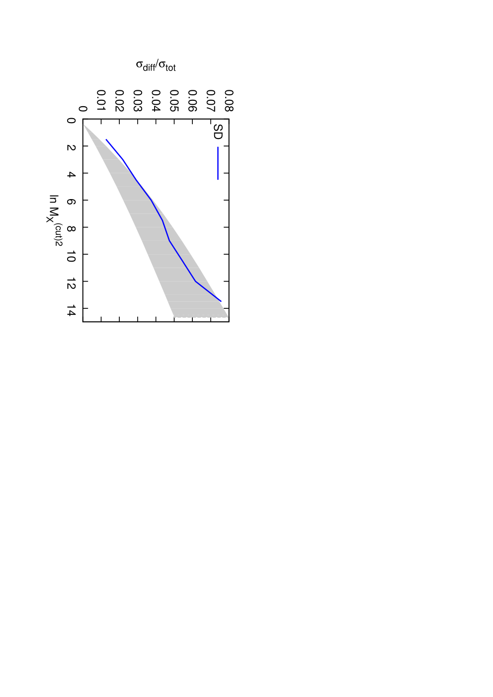
Diffractive excitation accounts for large fractions of the cross sections in DIS and collisions. As mentioned in Sec. 5.3, diffractive excitation is in the Good–Walker formalism determined by the fluctuations in the scattering amplitude, and we note that the BFKL evolution gives large fluctuations in the cascade evolution.
Study the interaction in a frame, where the projectile is evolved a distance and the target , with the total rapidity range . If we here first take the average over the target states, we get the amplitude for elastic scattering of the target. Squaring it gives the cross section, when the target is scattered elastically. If we after this take the average over the projectile states, we obtain the diffractive scattering of the projectile, including the elastic scattering. Thus the expression
| (41) |
gives the cross section for single diffractive excitation of the projectile, with the excited mass limited to . Varying gives then . The resulting cross sections for diffractive excitation in DIS and collisions are shown in Fig. 14, together with Zeus data for DIS, and an estimate from CDF data for collisions.

It is interesting to study the effects of saturation on diffractive excitation [32]. Saturation is not very important in DIS, but in scattering the Born amplitude is large, and therefore the unitarity effects are also large. Fig. 15 shows both the Born amplitude and the unitarized amplitude at 2 TeV for different impact parameters . We see that the width of the Born amplitude is very large, and without unitarization the fraction of diffractive excitation would be correspondingly large. (The smooth lines are fits of the form .)


However, the unitarized amplitude is limited by 1, and the width of the distribution, and therefore the diffractive excitation, is very much reduced. This result corresponds to the effect of enhanced diagrams in the conventional triple-regge approach. We note here also that the strong suppression from saturation implies that factorization is broken when comparing diffraction in collisions and DIS [35].
The absorption is most important for central collisions, where thus diffractive excitation is most strongly suppressed. As shown in Fig. 16, the cross section for diffractive excitation is therefore largest in a ring with radius , which grows slowly with energy.

6.3.3 Comparison with Multi-Regge Analyses
It is also interesting to compare the results from the Good–Walker analysis with the multi-regge formalism. To this end we study the contribution from the bare pomeron, meaning the one-pomeron amplitude without contributions from saturation, enhanced diagrams or gap survival form factors.
When , , and are all large, pomeron exchange should dominate. If the pomeron is a simple pole, we expect the following expressions for the total and diffractive cross sections:
| (42) |
Here is the pomeron trajectory, and and are the proton-pomeron and triple-pomeron couplings respectively. Comparing our result with this expression we find that it indeed reproduces the triple pomeron form, with the following parameter values obtained choosing the value for the arbitrary scale parameter [32]:
| (43) |
6.3.4 Correlations
We define the double parton distribution, and the impact parameter profile by the relation
| (44) |
where is the single parton distribution. This implies that the cross section for double hard interactions at midrapidity is given by
| (45) |
with the “effective cross section”, , determined by the relation
| (46) |
and are often assumed to depend only weakly on and . The DIPSY MC shows instead that a spike (hotspot) develops for small separations at larger , as illustrated in Fig. 17 [36]. This result implies that depends strongly on for fixed , as illustrated in Table 1. Part of the correlation is due to fluctuations in the cascade, which can also be taken into account in the MC. Without fluctuations should be 1. In Table 1 we see that the fluctuations increase by about 10%, which thus contributes to the correlations given by .


| [mb] | |||||
| 1.5 TeV, midrapidity | |||||
| 10 | 10 | 0.001 | 0.001 | 35.3 | 1.09 |
| 0.01 | 0.01 | 23.1 | 1.06 | ||
| 15 TeV, midrapidity | |||||
| 10 | 10 | 0.0001 | 0.0001 | 40.4 | 1.11 |
| 0.001 | 0.001 | 26.3 | 1.07 | ||
| 0.01 | 0.01 | 19.6 | 1.03 | ||
6.3.5 Final states
In order to generate exclusive final states, obtained when two dipole cascades collide, we first have to determine which dipoles interact and become recoupled in the way shown in Fig. 9. We note here that BFKL is a stochastic process, and the interactions between different dipole pairs are uncorrelated. This implies that the probability for interaction between dipoles and is given by , where is determined by Eq. (40).
As mentioned above, the BFKL equation describes the density of partons in a cascade, which is relevant for inclusive cross sections. To describe exclusive final states it is necessary to take into account colour coherence and angular ordering as well as soft radiation. The latter includes also contributions from the singularity in the gluon splitting function. These effects are taken into account in the CCFM formalism [12, 13], which also reproduces the BFKL result for the inclusive cross section.
A very schematic picture of a collision between two dipole cascades is presented in Fig. 18. Here three dipole pairs interact, forming two dipole loops with an additional loop (denoted ) formed within the evolution of the left cascade. Non-interacting branches, like and , have to be regarded as virtual and must be reabsorbed.

A reformulation of the CCFM model, called the Linked Dipole Chain model, was presented in Ref. [37]. Here it was demonstrated that the inclusive cross section is fully determined by a subset of the gluons in the CCFM approach, denoted “-changing” gluons. In Fig. 19a, we denote the real emitted gluons in a ladder , and the virtual links . The -changing emissions are either much larger or much smaller than . This also means that .
The chain in Fig. 19a is shown in the triangular phase space diagram in Fig. 19b. The real gluons are ordered in and in , and thus also in rapidity or angle. It was also demonstrated that to get the full final states, softer emissions have to be added below the horizontal lines in Fig. 19b, as final state radiation. This also includes the folds sticking out of the plane, which represent the transverse jets formed by the gluons .
Thus in order to generate exclusive final states we should go through the following steps:
1. Generate cascades for projectile and target
2. Determine which dipoles interact
3. Absorb non-interacting chains
4. Determine final state radiation
5. Hadronize
The main problems in this process are due to the large number of small dipoles in the cascades. These have low cross sections, and are therefore not a big problem for inclusive cross sections. Because small dipoles correspond to high transverse momenta, they do, however, have a large effect on the properties of the final states. This implies that the result is sensitive to details in the treatment of non-interacting dipoles. Our aim is here therefore not to give very precise predictions, but rather to get insight into the dynamical features of small evolution and saturation.
As a few examples Figs. 20 and 21 show comparisons with ATLAS data for minimum bias and underlying events at 0.9 and 7 TeV. Fig. 20 shows the -distribution of charged particles in minimum bias events. The solid line shows the result from the DIPSY MC, and the dotted line the result from Pythia. We note that the particle density is well reproduced at 0.9 TeV, but does not grow fast enough with energy, which is a problem also for other MCs which are not tuned individually for each energy. The properties of the underlying event is shown in Fig. 21, which presents the charged multiplicity in the “transverse region”, as defined by Rick Field, as a function of the of a leading charged particle. The model reproduces quite well the increased density for higher . More comparisons are found in Ref. [25].


6.3.6 Nucleus collisions
The model can also be applied to reactions involving nuclei, where e.g. saturation effects can be studied including a proper geometry. Some early results are presented in Ref. [40].
7 Summary
In these lectures I have discussed interaction cross sections and particle production in -ann., DIS, and high energy hadronic collisions. It includes hadronization, initial and final state radiation, small evolution and saturation.
I have also presented the Lund Dipole Cascade model for high energy collisions, which is based on BFKL evolution and saturation. It is an extension of Mueller’s model, also including
- •
important non-leading effects in BFKL
- •
saturation within the evolution
- •
confinement
- •
A MC implementation DIPSY
The model gives a good description of inclusive and cross sections (including diffraction), and a fair description of exclusive final states (min. bias and underlying event). It has fewer tunable parameters than other event generators, and our aim is not to give very precise predictions, but rather to get insight into the dynamical features of small evolution and saturation. As examples it is here possible to study effects of correlations, fluctuations, and finite transverse size in a way, which is not easy in other approaches.
References
- [1] J. K. Jackson, Classical Electrodynamics, John Wiley & Sons, 1998.
- [2] R. K. Ellis, D. A. Ross, A. E. Terrano, Nucl. Phys. B178 (1981) 421.
- [3] Y. I. Azimov, Y. L. Dokshitzer, V. A. Khoze, S. I. Troian, Phys. Lett. B165 (1985) 147-150.
- [4] G. Gustafson, U. Pettersson, Nucl. Phys. B306 (1988) 746.
- [5] L. Lönnblad, Comput. Phys. Commun. 71 (1992) 15-31.
- [6] G. Gustafson, A. Nilsson, Nucl. Phys. B355 (1991) 106-122.
- [7] B. Andersson, G. Gustafson, B. Söderberg, Z. Phys. C20 (1983) 317.
- [8] B. Andersson, G. Gustafson, Z. Phys. C3 (1980) 223.
- [9] B. Andersson, G. Gustafson, T. Sjöstrand, Phys. Lett. B94 (1980) 211.
- [10] JADE Coll., Phys. Lett. B157 (1985) 340, Z. Phys. C39 (1988) 1.
- [11] A.H. Mueller, Nucl. Phys. B415 (1994) 373.
- [12] S. Catani, F. Fiorani, G. Marchesini, Nucl. Phys. B336 (1990) 18.
- [13] M. Ciafaloni, Nucl. Phys. B296 (1988) 49.
- [14] T. Akesson et al. [ Axial Field Spectrometer Collaboration ], Z. Phys. C34 (1987) 163.
- [15] F. Abe et al. [ CDF Collaboration ], Phys. Rev. D47 (1993) 4857-4871.
- [16] F. Abe et al. [ CDF Collaboration ], Phys. Rev. D56 (1997) 3811-3832.
- [17] V. M. Abazov et al. [ D0 Collaboration ], Phys. Rev. D67 (2003) 052001. [hep-ex/0207046].
- [18] R. Field, arXiv:1110.5530 [hep-ph].
- [19] Y. V. Kovchegov, Phys. Rev. D61 (2000) 074018. [hep-ph/9905214].
- [20] A.H. Mueller and B. Patel, Nucl. Phys. B425 (1994) 471 [hep-ph/9403256].
- [21] A.H. Mueller, Nucl. Phys. B437 (1995) 107 [hep-ph/9408245].
- [22] E. Avsar, G. Gustafson, L. Lönnblad, JHEP 0507 (2005) 062. [hep-ph/0503181].
- [23] E. Avsar, G. Gustafson, and L. Lönnblad, JHEP 01 (2007) 012 [hep-ph/0610157].
- [24] C. Flensburg, G. Gustafson, L. Lönnblad, Eur. Phys. J. C60 (2009) 233-247. [arXiv:0807.0325 [hep-ph]].
- [25] C. Flensburg, G. Gustafson, L. Lönnblad, JHEP 1108 (2011) 103 [arXiv:1103.4321 [hep-ph]].
- [26] G. P. Salam, Acta Phys. Polon. B30 (1999) 3679-3705. [hep-ph/9910492].
- [27] J. Kwiecinski, A. D. Martin, P. J. Sutton, Z. Phys. C71 (1996) 585-594. [hep-ph/9602320].
- [28] I. Balitsky and G. A. Chirilli, Acta Phys. Polon. B 39 (2008) 2561.
- [29] E. Avsar, JHEP 0804 (2008) 033. [arXiv:0803.0446 [hep-ph]].
- [30] A. M. Stasto, K. J. Golec-Biernat and J. Kwiecinski, Phys. Rev. Lett. 86 (2001) 596 [hep-ph/0007192].
- [31] A. Aktas et al. [H1 Collaboration], Eur. Phys. J. C 44 (2005) 1 [hep-ex/0505061].
- [32] C. Flensburg and G. Gustafson, JHEP 1010 (2010) 014 [arXiv:1004.5502 [hep-ph]].
- [33] S. Chekanov et al. [ZEUS Collaboration], Nucl. Phys. B 713 (2005) 3 [hep-ex/0501060].
- [34] F. Abe et al. [CDF Collaboration], Phys. Rev. D 50 (1994) 5535.
- [35] F. -P. Schilling [H1 Collaboration], Acta Phys. Polon. B 33 (2002) 3419 [hep-ex/0209001].
- [36] C. Flensburg, G. Gustafson, L. Lönnblad, A. Ster, JHEP 1106 (2011) 066. [arXiv:1103.4320 [hep-ph]].
- [37] B. Andersson, G. Gustafson, J. Samuelsson, Nucl. Phys. B467 (1996) 443-478.
- [38] G. Aad et al. [ ATLAS Collaboration ], New J. Phys. 13 (2011) 053033. [arXiv:1012.5104 [hep-ex]].
- [39] G. Aad et al. [ Atlas Collaboration ], Phys. Rev. D 83 (2011) 112001. [arXiv:1012.0791 [hep-ex]].
- [40] C. Flensburg, arXiv:1108.4862 [nucl-th].