On hybrid models of quantum finite automata

In the literature, there is a class of QFA that differ from other QFA models by consisting of two interactive components: a quantum component and a classical one. We call them hybrid models of QFA in this paper. These hybrid models are of particular interest, as they show praiseworthy advantages over the fully quantum models in some nontrivial aspects.

The first hybrid model of QFA is the two-way quantum finite automata with quantum and classical states (2QCFA, for short) proposed by Ambainis and Watrous [4] in which on scanning an input symbol, the internal states evolve as follows: first the quantum part undergoes a unitary operator or a projective measurement that is determined by the current classical state and the scanned symbol, and then the classical part specifies a new classical state and a movement of the tape head (left, right, or stationary), which depends on the scanned symbol (along with the outcome if the quantum part makes a measurement). In [4], it was shown that 2QCFA are strictly more powerful than their classical counterparts—two-way probabilistic finite automata (2PFA). In this paper we will discuss a one-way variant of 2QCFA, denoted by 1QCFA (where the tape head is restricted to move towards only right).

Another hybrid model in the literature is the one-way quantum finite automata with control language (CL-1QFA, for short) proposed by Bertoni [6] in which on scanning an input symbol, a unitary operator followed by a projective measurement is applied to the current quantum state. Thus, a CL-1QFA fed with an input string $x$ finally produces a sequence $y$ of measurement results with a certain probability. The input string $x$ is said to be accepted if $y$ is in a given regular language (i.e., the control language). It was shown in [6, 17] that CL-1QFA recognize exactly the class of regular languages, and CL-1QFA can be more succinct (i.e., have less states) than deterministic finite automata (DFA) for certain languages.

Very recently, Qiu et al [25] proposed a new hybrid model called 1QFA together with classical states (1QFAC, for short) which consists of a quantum component and a classical one. On scanning an input symbol, the two components interact in the following way: first the quantum component undergoes a unitary operator that is determined by the current classical state and the scanned symbol, and then the classical component evolves like a DFA. After scanning the whole input string, a projective measurement determined by the final classical state is performed on the final quantum state, giving the accepting and rejecting probabilities. In [25], it was proved that 1QFAC recognize all regular languages and are exponentially more concise than DFA for certain languages.

The hybrid models mentioned above are of particular interest and worthy of further consideration, at least for the following reasons. First, hybrid models are easier to be physically implemented than fully quantum models. For example, while the position of the tape head in the 2QFA model introduced by Kondacs and Watrous [11] is a superposed quantum state and at least $O(\log n)$ qubits are required to store it (where $n$ is the length of the input), in a 2QCFA the tape head position is merely a classical variable which is easy to store and manipulate. Second, hybrid models often save states by being augmented with a small number of quantum states. For example, CL-1QFA and 1QFAC have been proved to be much smaller than DFA when accepting the same language. Therefore, it is beneficial to construct a hybrid model for a practical problem (language) with an appropriate trade-off between quantum and classical states. Last but not least, quantum engineering systems developed in the further will most probably have a classical human-interactive interface and a quantum processor, and thus they are hybrid models. In fact, hybrid models have already been encountered several times in quantum computing, varying from quantum Turing machines [27] and quantum finite automata [4, 6, 25] to multiple-prover quantum interactive proof systems (the model of complexity class MIP^∗ [8]) and quantum programming [28].²² 2 As stated by Selinger [28], quantum programs can be described by “quantum data with classical control flows”. Thus, a quantum program can be viewed as a hybrid model where quantum data are represented by states of a quantum component and classical control flows are implemented by a classical component.

This paper aims to characterize the structure of these hybrid models in a uniform framework and to clarify the relationship between these models and others. The contribution of this paper is as follows. (i) First, we characterize three hybrid models of QFA (1QCFA, CL-1QFA, and 1QFAC ) in a uniform framework: each hybrid QFA is represented as a communication system consisting of a quantum component and a classical one with the communication between them modeled by controlled operations. The three models differ from each other only in the specific communication pattern. (ii) Second, we will show that 1QCFA, CL-1QFA, and 1QFAC can all be simulated exactly by 1QFA with quantum operations. 1QFA with quantum operations actually represent the same model as another early proposed model—ancilla QFA, which in turn can be regarded as quantum sequence machines assigned with some accepting states. We refer to Fig. 1 for their detailed relationship.

The reminder of this paper is organized as follows. Some preliminaries from quantum theory, automata theory and controlled operations are presented in Section 2. In Section 3 we characterize the structure of three hybrid models of QFA in a uniform framework. Section 4 clarifies the relationship between hybrid models of QFA and other models. Some results concerning the language recognition power and the equivalence problem of hybrid QFA follow as corollaries there. Some conclusions are made in Section 5.

For convenience of the reader we briefly recall some basic notions from quantum theory. We refer to [18] for more details. According to von Neumann’s formalism of quantum mechanics, a quantum system is associated with a Hilbert space which is called the state space of the system. In this paper, we only consider finite dimensional spaces. A (mixed) state of a quantum system is represented by a density operator on its state space. Here a density operator $\rho$ on ${\cal H}$ is a positive semi-definite linear operator such that $\text{Tr}(\rho)=1$. When the rank of $\rho$ is $1$, that is, $\rho=|\psi\rangle\langle\psi|$ for some $|\psi\rangle\in{\cal H}$, then $\rho$ is called a pure state. Let $L({\cal H})$ and $D({\cal H})$ be the sets of linear operators and density operators on ${\cal H}$, respectively.

The evolution of a closed quantum system is described by a unitary operator $U$ on its state space. If the states of the system at times $t_{1}$ and $t_{2}$ are $\rho_{1}$ and $\rho_{2}$, respectively, then $\rho_{2}=U\rho_{1}U^{{\dagger}}$ for some unitary operator $U$ which depends only on $t_{1}$ and $t_{2}$. Here $U^{\dagger}$ is the complex conjugate and transpose of $U$.

In contrast, the evolution of an open quantum system is characterized by a quantum operation ${\cal E}$ on its state space ${\cal H}$, which is a linear map from $L(\mathcal{H})$ to itself that has an operator-sum representation as

where $\{E_{k}\}$, known as the operation elements of ${\cal E}$, are linear operators on ${\cal H}$. Furthermore, ${\cal E}$ is said to be trace-preserving if the following completeness condition is satisfied:

Throughout the rest of this paper, when referring to a quantum operation ${\cal E}$, it is always assumed to be trace-preserving.

To extract information from a quantum system, a measurement has to be performed. A general measurement is described by a collection $\{M_{m}\}$ of measurement operators, where the index $m$ refers to the potential measurement outcome, satisfying the completeness condition

If this measurement is performed on a state $\rho$, then the classical outcome $m$ is obtained with the probability $p(m)=\text{Tr}(M_{m}^{\dagger}M_{m}\rho)$, and the post-measurement state is

For the case that $\rho$ is a pure state $|\psi\rangle$, that is, $\rho=|\psi\rangle\langle\psi|$, we have $p(m)=\|M_{m}|\psi\rangle\|^{2},$ and the state $|\psi\rangle$ “collapse” into the state

A special case of general measurements is the projective measurement $\{P_{m}\}$ where $P_{m}$’s are orthogonal projectors.

Suppose we have physical systems $A$ and $B$, whose state is described by a density operator $\rho^{AB}\in D({\cal H}_{A}\otimes{\cal H}_{B})$. Then the state for system $A$ is $\rho^{A}=\text{Tr}_{B}(\rho^{AB})$ where $\text{Tr}_{B}$, known as the partial trace over system $B$, is defined by a linear map from ${\cal H}_{A}\otimes{\cal H}_{B}$ to ${\cal H}_{A}$ satisfying

where $|a_{1}\rangle,|a_{2}\rangle\in{\cal H}_{A}$, and $|b_{1}\rangle,|b_{2}\rangle\in{\cal H}_{B}$.

For a non-empty set $\Sigma$, denote by $\Sigma^{k}$ and $\Sigma^{*}$ the sets of all strings over $\Sigma$ with length $k$ and with finite length, respectively. Let $|w|$ be the length of string $w$.

A DFA is a five-tuple ${\cal A}=(S,\Sigma,s_{1},\delta,S_{a})$ where $S$ is a finite state set, $\Sigma$ is a finite alphabet, $s_{1}\in S$ is the initial state, $S_{a}\subseteq S$ is the accepting set, and $\delta:S\times\Sigma\rightarrow S$ is the transition function³³ 3 Without loss of generality, $\delta$ is required to be a total function.: $\delta(s,\sigma)=t$ means that the current state $s$ changes to $t$ when scanning $\sigma$. Furthermore, $\delta$ can be extended to $\delta^{*}:S\times\Sigma^{*}\rightarrow S$ by defining: i) $\delta^{*}(s,\epsilon)=s$, and ii) $\delta^{*}(s,x\sigma)=\delta(\delta^{*}(s,x),\sigma)$ where $x\in\Sigma^{*}$ and $\sigma\in\Sigma$. ${\cal A}$ is said to accept $x\in\Sigma^{*}$, if $\delta^{*}(s_{1},x)\in S_{a}$.

We can also describe a DFA using the matrix notation. Let $A_{\sigma}$ be an $|S|\times|S|$ matrix with $A_{\sigma}[i,j]$ being $1$ if $\delta(s_{j},\sigma)=s_{i}$, and $0$ otherwise. Then each column of $A_{\sigma}$ has a unique $1$ and other entries are all 0. Let $\pi$ be a 0-1 column vector with only the first entry being $1$, and $\eta$ the 0-1 row vector with $\eta_{i}=1$ iff $s_{i}\in S_{a}$. Define a function $f_{A}:\Sigma^{*}\rightarrow\{0,1\}$ as

Then $f_{A}(x)=1$ iff $A$ accepts $x$.

Let ${\cal H}_{A}\otimes{\cal H}_{B}$ be the state space of a bipartite quantum system $AB$. Let $\{P_{i}\}_{i=1}^{n}$ be a projective measurement on ${\cal H}_{A}$ with $n$ outcomes, and $\mathcal{E}_{i}$, $1\leq i\leq n$, quantum operations on ${\cal H}_{B}$. The controlled operation ‘if subsystem $A$ was measured in result $i$, then $\mathcal{E}_{i}$ is performed on subsystem $B$’ can be defined by the following operation elements

where $\{E^{i}_{k}\}_{k\in K_{i}}$ are operation elements of $\mathcal{E}_{i}$, that is, $\mathcal{E}_{i}(\rho)=\sum_{k\in K_{i}}E^{i}_{k}\rho{E^{i}_{k}}^{\dagger}$. It is straightforward to check that the elements in (3) satisfy the completeness condition. Furthermore, for $\rho\otimes\varrho\in L({\cal H}_{A}\otimes{\cal H}_{B})$, we have

If the projective measurement $\{P_{i}\}_{i=1}^{n}$ in the above is replaced by a general measurement $\{M_{i}\}_{i=1}^{n}$, then we get a quantum operation $\mathcal{E}^{\prime}$ that has the following effect

Hybrid models discussed in this paper are depicted in Fig. 2. A hybrid model of QFA comprises a quantum component, a classical component, a classical communication channel, and a classical tape head (that is, the tape head is regulated by the classical component). On scanning an input symbol, the quantum and classical components interact to evolve into new states, during which communication may occur between them. In this paper, we focus on hybrid models with a one-way tape head, that is, on scanning an input symbol the model moves its tape head one cell right.

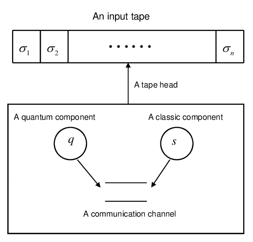
In the literature there are three models of QFA (CL-1QFA, 1QFAC, and 2QCFA) fitting into Fig. 2. For the last model, we will consider its on-way variant 1QCFA. We will show that these models can be characterized in a uniform framework as in Fig. 2, with the only difference being the specific communication pattern:

• 1.

  In CL-1QFA, only quantum-classical communication is allowed, that is, the quantum component sends its measurement result to the classical component, but no reverse communication is permitted.

• 2.

  In 1QFAC, only classical-quantum communication is allowed, that is, the classical component sends its current state to the quantum component.

• 3.

  In 1QCFA, two-way communication is allowed: (1) first, the classical component sends its current state to the quantum component; (2) second, the quantum component sends its measurement result to the classical component.

Throughout the remainder of this paper we let ${\cal H}_{Q}$, where $Q=\{q_{1},q_{2},\cdots,q_{n}\}$, be the n-dimensional Hilbert space spanned by the orthonormal vectors $\{|q_{i}\rangle:i=1,\cdots,n\}$. Mathematically, $|q_{i}\rangle$ is an $n$-dimensional column vector having $1$ as the $i$th entry and $0$ else. Sometimes we abuse the notation slightly by writting $q_{i}$ directly for $|q_{i}\rangle$.

Bertoni et al [6] introduced a QFA model called one-way QFA with control language (CL-1QFA), defined as follows.

In CL-1QFA ${\cal A}$, on scanning a symbol $\sigma$, a unitary operator $U_{\sigma}$ followed by the projective measurement $\mathcal{M}$ is performed on its current state. Thus, given an input string $x\in\Sigma^{*}$, the computation produces a sequence $y\in{\cal C}^{*}$ of measurement results with a certain probability $p(y|x)$ that is given by

where we define the ordered product $\prod_{i=1}^{n}A_{i}=A_{n}A_{n-1}\cdots A_{1}$. The computation is said to be accepted if $y$ belongs to a fixed regular language ${\cal L}\subseteq{\cal C}^{*}$. Thus the probability of ${\cal M}$ accepting $x$ is

Obviously, a CL-1QFA can be regarded as a hybrid model comprising the following two components:

• 1.

  A quantum component with state space ${\cal H}_{Q}$ that undergos unitary operators $\{U_{\sigma}\}$ and projective measurement ${\cal M}$.

• 2.

  A classical component that is the DFA accepting the control language ${\cal L}$.

Note that the classical DFA accepting ${\cal L}$ takes the measurement outcomes of the quantum component as input. Thus, communication occurs from the quantum component to the classical one. The structure of CL-1QFA is illustrated in Fig. 3.

Recently, Qiu et al [25] proposed a new model named 1QFA together with classical states (1QFAC), defined as follows.⁴⁴ 4 In this paper we consider only the case that 1QFAC are language acceptors, and one can refer to [25] for a more general definition.

The machine starts with the initial states $s_{1}$ and $q_{1}$. On scanning an input symbol $\sigma\in\Sigma$, $U_{s,\sigma}$ is first applied to the current quantum state, where $s$ is the current classical state; afterwards, the classical state $s$ changes to $t=\delta(s,\sigma)$. Finally, when the whole input string is finished, a measurement ${\cal M}_{s}$ determined by the final classical state is performed on the final quantum state, and the input is accepted if the outcome $a$ is observed. Therefore, the probability of 1QFAC ${\cal A}$ accepting $x=x_{1}x_{2}\cdots x_{n}\in\Sigma^{*}$ is given by

where $s_{i+1}=\delta(s_{i},x_{i})$ for $i=1,\cdots,n$.

Again, it is easy to see that a 1QFAC is actually a hybrid model comprising the follows two components:

• 1.

  A quantum component with state space ${\cal H}_{Q}$, undergoing unitary operators $\{U_{s,\sigma}\}$.

• 2.

  A classical component represented by a DFA ${\cal A}^{\prime}=(S,\Sigma,s_{1},\delta)$ without an accepting set.

Note that each unitary operator $U_{s,\sigma}$ is determined by the current classical state $s$. Thus, communication is required from the classical component to the quantum one. The structure of 1QFAC is illustrated in Fig. 4.

Ambainis and Watrous [4] proposed the model of two-way QFA with quantum and classical states (2QCFA). As proved in [4], 2QCFA can recognize non-regular language $L_{eq}=\{a^{n}b^{n}|n>0\}$ in polynomial time and the palindrome language $L_{pal}=\{x\in\{a,b\}^{*}|x=x^{R}\}$ in exponential time, which shows the superiority of 2QCFA over their classical counterparts 2PFA. In the following we discuss 1QCFA, the one-way variant of 2QCFA.

The notion of 1QCFA given above is slightly more general than the one-way version of 2QCFA in [4], where each $\Theta_{s,\sigma}$ is required to be either a unitary operator or a projective measurement, both being special cases of general measurement considered here.

On scanning a symbol $\sigma$, first the general measurement $\Theta_{s,\sigma}$ determined by the current classical state $s$ and the scanned symbol $\sigma$ is performed on the current quantum state, producing some outcome $c\in{\cal C}$; then the classical state $s$ changes to $s^{\prime}=\delta(s,\sigma,c)$ by reading $\sigma$ and $c$. After scanning all input symbols, ${\cal A}$ checks whether its classical state is in $S_{a}$. If yes, the input is accepted; otherwise, rejected. Therefore, the probability of 1QCFA ${\cal A}$ accepting $x=x_{1}x_{2}\cdots x_{n}\in\Sigma^{*}$ is given by

where:

• (1)

  $\chi_{a}:S\rightarrow\{0,1\}$ is defined by $\chi_{a}(s)=\left\{\begin{array}[]{ll}1,&\hbox{if $s\in S_{a}$;}\\ 0,&\hbox{otherwise.}\end{array}\right.$

• (2)

  $\{M^{c}_{s,\sigma}\}_{c\in{\cal C}}$ are measurement operators of $\Theta_{s,\sigma}$.

• (3)

  $s_{i+1}=\delta(s_{i},x_{i},c_{i})$ for $i=1,\cdots,n$.

Obviously, a 1QCFA is a hybrid model comprising the following two components:

• 1.

  A quantum component with state space ${\cal H}_{Q}$, undergoing general measurements $\{\Theta_{s,\sigma}\}$ with outcome set ${\cal C}$.

• 2.

  A classical component represented by a DFA ${\cal A}^{\prime}=(S,\Sigma\times{\cal C},s_{1},\delta,S_{a})$.

Note that two-way communication occurs between the two components, since each $\Theta_{s,\sigma}$ is determined by the classical state $s$ and the DFA ${\cal A}^{\prime}$ has to scan the outcome $c$ produced by the quantum component. The structure of 1QCFA is illustrated in Fig. 5.

In the following, we recall the definition of MO-1gQFA.

On scanning a symbol $\sigma$, the quantum operation ${\cal E}_{\sigma}$ is performed on the current state. After the operation corresponding to the last symbol is performed, a projective measurement is applied to determine acceptance. Thus, for the input string $x=\sigma_{1}\sigma_{2}\cdots\sigma_{n}\in\Sigma^{*}$, ${\cal A}$ produces the accepting probability given by

where ${\cal E}_{2}\circ{\cal E}_{1}(\rho)$ stands for ${\cal E}_{2}({\cal E}_{1}(\rho))$.

MO-1gQFA have been thought to be a nice definition of QFA, since they possess nice closure properties and have a competitive computational power with their classical counterparts. The next lemma shows that any DFA can be simulated by a MQ-1gQFA.

Proof. Let $E_{s}^{\sigma}=|\delta(s,\sigma)\rangle\langle s|$ where $s\in S$ and $\sigma\in\Sigma$. Then for each $\sigma\in\Sigma$, we get a quantum operation $\mathcal{E}_{\sigma}$ given by $\mathcal{E}_{\sigma}(\rho)=\sum_{s\in S}E_{s}^{\sigma}\rho{E_{s}^{\sigma}}^{\dagger}$. By a direct calculation, it is easy to verify that $|t\rangle\langle t|=\mathcal{E}_{\sigma}(|s\rangle\langle s|)$ iff $t=\delta(s,\sigma)$. Then the claimed result can be obtained by induction on the length of the input string. ∎

From the above lemma, it can be seen that $P_{{\cal A}^{\prime}}(x)=1$ if ${\cal A}$ accepts $x$ and $P_{{\cal A}^{\prime}}(x)=0$ if not. As a result, for each regular language there exists an MO-1gQFA which recognizes it with certainty. A full characterization of the languages recognized by MO-1gQFA is as follows.

In the following, we show that for a given CL-1QFA, there exists an MO-1gQFA simulating it.

Proof. Let ${\cal A}=(Q,\Sigma,{\cal C},q_{1},\{U_{\sigma}\}_{\sigma\in\Sigma},\mathcal{M},{\cal L})$ be a CL-1QFA. As shown in Section 3.2, ${\cal A}$ is a hybrid model with a quantum component $Q$ and a classical component being a DFA $\mathcal{A}^{\prime}=(S,{\cal C},s_{1},\delta,S_{a})$ accepting ${\cal L}$. The idea of the simulation is to encode the communication from $Q$ to $\mathcal{A}^{\prime}$ into a controlled operation introduced in Section 2.3.

First by Lemma 1, there exists an MO-1gQFA $\mathcal{A}^{\prime\prime}=(S,\mathcal{C},s_{1},\{\mathcal{F}_{c}\}_{c\in{\cal C}},S_{a})$, in which each $\mathcal{F}_{c}$ on $\mathcal{H}_{S}$ is represented by operation elements $\{F^{s}_{c}\}_{s\in S}$ with $F^{s}_{c}=|\delta(s,c)\rangle\langle s|$, such that $|t\rangle\langle t|=\mathcal{F}_{c}(|s\rangle\langle s|)$ iff $t=\delta(s,c)$.

Now we construct an MO-1gQFA

from $\mathcal{A}$ and $\mathcal{A}^{\prime\prime}$ as follows:

• 1.

  $\widehat{Q}=Q\times S$;

• 2.

  $\widehat{q}_{1}=(q_{1},s_{1})$;

• 3.

  $\widehat{Q}_{a}=Q\times S_{a}$, associated with the projector $\widehat{P}_{a}=I_{Q}\otimes\sum_{s\in S_{a}}|s\rangle\langle s|$ where $I_{Q}$ is the identity operator on ${\cal H}_{Q}$;

• 4.

  for each $\sigma\in\Sigma$, $\widehat{\mathcal{E}}_{\sigma}$ has operation elements $\{\widehat{E}_{\sigma}^{c,s}\}_{c\in\mathcal{C},s\in S}$ where

  $$\widehat{E}_{\sigma}^{c,s}=P_{c}U_{\sigma}\otimes F_{c}^{s}=P_{c}U_{\sigma}\otimes|\delta(s,c)\rangle\langle s|.$$

  It is easy to verify that the collection $\{\widehat{E}_{\sigma}^{c,s}\}$ satisfies the completeness condition. Furthermore, for $\rho\otimes\varrho\in L(\mathcal{H}_{Q}\otimes\mathcal{H}_{S})$, we have

  $$\widehat{\mathcal{E}}_{\sigma}(\rho\otimes\varrho)=\sum_{c\in\mathcal{C}}P_{c}U_{\sigma}\rho U_{\sigma}^{\dagger}P_{c}\otimes\mathcal{F}_{c}(\varrho).$$

Now let us check the behavior of $\widehat{\cal A}$ on an input string. Suppose $\widehat{\cal A}$ starts with the initial state $(q_{1},s_{1})$ and scans a symbol $\sigma$. Then the result state is

where $t_{c}=\delta(s_{1},c)$. In this way, after scanning a string $x=x_{1}x_{2}\cdots x_{n}\in\Sigma^{*}$, the final state is

where $|\phi_{y}\rangle=\prod_{i=1}^{n}(P_{y_{i}}U_{x_{i}})|q_{1}\rangle$ and $s_{y}=\delta^{*}(s_{1},y)$. Note that $s_{y}\in S_{a}$ iff $y\in{\cal L}$. Thus the probability of $\widehat{\cal A}$ accepting $x$ is

where $\chi_{a}(s)$, defined after Eq. (7), indicates whether $s$ is in $S_{a}$. Note that the above probability is equal to the one of ${\cal A}$ given in Eq. (5). Therefore, we have completed the proof.∎

By a similar idea as before, we can simulate 1QFAC by MO-1gQFA.

Proof. Let ${\cal A}=(Q,S,\Sigma,q_{1},s_{1},\{U_{s,\sigma}\}_{s\in S,\sigma\in\Sigma},\delta,\{{\cal M}_{s}\}_{s\in S})$ be a 1QFAC. As shown in Section 3.3, ${\cal A}$ is a hybrid model with a quantum component $Q$ and a classical component being a DFA ${\cal A}^{\prime}=(S,\Sigma,s_{1},\delta)$ without an accepting set. The idea of the simulation is to encode the communication from ${\cal A}^{\prime}$ to $Q$ into a controlled operation introduced in Section 2.3.

First by Lemma 1, there exists an MO-1gQFA ${\cal A}^{\prime\prime}=(S,\Sigma,s_{1},\{\mathcal{F}_{\sigma}\}_{\sigma\in\Sigma})$ (without an accepting set), such that $|t\rangle\langle t|=\mathcal{F}_{\sigma}(|s\rangle\langle s|)$ iff $t=\delta(s,\sigma)$. Then we construct an MO-1gQFA

as follows:

• 1.

  $\widehat{Q}=S\times Q$;

• 2.

  $\widehat{q}_{1}=(s_{1},q_{1})$;

• 3.

  For each $\sigma\in\Sigma$, $\widehat{\mathcal{E}}_{\sigma}$ on $\mathcal{H}_{S}\otimes\mathcal{H}_{Q}$ is given by

  $$\widehat{\mathcal{E}}_{\sigma}=(\mathcal{F}_{\sigma}\otimes\mathcal{I})\circ\mathcal{E}_{\sigma}$$

  where $\mathcal{I}$ is the identity mapping on $L(\mathcal{H}_{Q})$, and $\mathcal{E}_{\sigma}$ is given by operation elements $\{E_{s}=|s\rangle\langle s|\otimes U_{s,\sigma}\}_{s\in S}$. Given $\rho\otimes\varrho\in L(\mathcal{H}_{S}\otimes\mathcal{H}_{Q})$, we have

  $$\widehat{\mathcal{E}}_{\sigma}(\rho\otimes\varrho)=\sum_{s\in S}\langle s|\rho|s\rangle\mathcal{F}_{\sigma}(|s\rangle\langle s|)\otimes U_{s,\sigma}\varrho U_{s,\sigma}^{\dagger},$$

  which captures the idea that if the current classical state is $s$, then $U_{s,\sigma}$ is performed on the quantum component, and furthermore $s$ changes to another state according to $\mathcal{F}_{\sigma}$.

• 4.

  Instead of specifying the set of accepting states,⁷⁷ 7 Specifying an accepting state set is essentially equivalent to specifying a projective measurement. we specify here the final projective measurement $\{\widehat{P}_{a},\widehat{P}_{r}\}$. Suppose ${\cal M}_{s}=\{P_{s,a},P_{s,r}\}$. We let

  $$\widehat{P}_{a}=\sum_{s_{i}\in S}|s_{i}\rangle\langle s_{i}|\otimes P_{s_{i},a}$$

  and

  $$\widehat{P}_{r}=\sum_{s_{i}\in S}|s_{i}\rangle\langle s_{i}|\otimes P_{s_{i},r}.$$

  It is easily verified that $\widehat{P}_{a}$ and $\widehat{P}_{r}$ form a projective measurement.

In the following we verify that $\widehat{\cal A}$ and ${\cal A}$ have the same accepting probability for any given input string. Let $\rho_{x}$ be the state of $\widehat{\cal A}$ after scanning $x$ and before the final measurement. Then by induction on the length of the input string, it is easy to show that for each $x=x_{1}x_{2}\cdots x_{n}\in\Sigma^{*}$, we have

with

1. (1)

   $|\psi_{x}\rangle=U_{s_{n},x_{n}}\cdots U_{s_{2},x_{2}}U_{s_{1},x_{1}}|q_{1}\rangle$, and

2. (2)

   $s_{i+1}=\delta(s_{i},x_{i})$ for $i=1,\cdots,n$.

Therefore, the probability of $\widehat{\mathcal{A}}$ accepting $x$ is

which is equal to the the accepting probability of ${\cal A}$ given in Eq. (7). This completes the proof of Theorem 2. ∎

In this section we show how 1QCFA can be simulated by MO-1gQFA. This simulation is more complicated than previous simulations of CL-1QFA and 1QFAC, since now two-way communication occurs in 1QCFA. However, the ideals are similar.

Proof. Let $\mathcal{A}=(Q,S,\Sigma,{\cal C},q_{1},s_{1},\{\Theta_{s,\sigma}\}_{s\in S,\sigma\in\Sigma},\delta,S_{a})$ be a 1QCFA. As shown in Section 3.4, $\mathcal{A}$ is a hybrid model comprising a quantum component $Q$ and a classical component being a DFA $\mathcal{A}^{\prime}=(S,\Sigma\times{\cal C},s_{1},\delta,S_{a})$. The idea of the simulation is to encode the communication between $Q$ and $A^{\prime}$ into a controlled operation introduced in Section 2.3.

First it follows from Lemma 1 that for the DFA $\mathcal{A}^{\prime}$, there exists an MO-1gQFA $\mathcal{A}^{\prime\prime}=(S,\Sigma\times{\cal C},s_{1},\{\mathcal{F}_{\sigma,c}\}_{\sigma,c\in\Sigma\times{\cal C}},S_{a}),$ such that $|t\rangle\langle t|=\mathcal{F}_{\sigma,c}(|s\rangle\langle s|)$ iff $t={\delta}(s,\sigma,c)$ for $(\sigma,c)\in\Sigma\times{\cal C}$. Then we construct an MO-1gQFA

as follows:

• 1.

  $\widehat{Q}=Q\times S$;

• 2.

  $\widehat{q}_{1}=(q_{1},s_{1})$;

• 3.

  $\widehat{Q}_{a}=Q\times S_{a}$, associated with the projector $\widehat{P}_{a}=I_{Q}\otimes\sum_{s\in S_{a}}|s\rangle\langle s|$;

• 4.

  Each $\widehat{\mathcal{E}}_{\sigma}$ on $\mathcal{H}_{Q}\otimes\mathcal{H}_{S}$ is given by the following operation elements

  $\displaystyle\{M^{c}_{s,\sigma}\otimes F^{k}_{\sigma,c}E_{s}:s\in S,c\in\mathcal{C},k\in K_{\sigma,c}\}$

  (8)

  where:

  • (a)

    $E_{s}=|s\rangle\langle s|$ for $s\in S$, which is used to detect whether the classical state is $s$;

  • (b)

    $\{M^{c}_{s,\sigma}\}_{c\in\mathcal{C}}$ are measurement operators of $\Theta_{s,\sigma}$;

  • (c)

    $\{F^{k}_{\sigma,c}\}_{k\in K_{\sigma,c}}$ are operation elements of $\mathcal{F}_{\sigma,c}$, that is, $\mathcal{F}_{\sigma,c}(\varrho)=\sum_{k\in K_{\sigma,c}}F^{k}_{\sigma,c}\varrho{F^{k}_{\sigma,c}}^{\dagger}$.

For each $\sigma\in\Sigma$, $\widehat{\mathcal{E}}_{\sigma}$ given by Eq. (8) satisfies the completeness condition

Furthermore, for $\rho\otimes\varrho\in L(\mathcal{H}_{Q}\otimes\mathcal{H}_{S})$, by a direct calculation we have

The above equation intuitively captures the idea that if the current classical state is $s$, then $\Theta_{s,\sigma}$ is performed on the quantum component; furthermore, if the outcome of $\Theta_{s,\sigma}$ is $c$, then $\mathcal{F}_{\sigma,c}$ is applied on the classical component. For example, given the initial state $|q_{1}\rangle|s_{1}\rangle$, we have

In the following, we verify that the constructed MO-1gQFA $\widehat{\cal A}$ and the given 1QCFA ${\cal A}$ have the same accepting probability for any given input string. Let $\rho_{x}$ be the state of $\widehat{\cal A}$ after scanning $x$ and before the final measurement. Then for $x=x_{1}x_{2}\cdots x_{n}\in\Sigma^{*}$, we have

References

- [1] A. Ambainis and R. Freivalds, One-way quantum finite automata: strengths, weaknesses and generalizations, in Proceedings of the 39th Annual Symposium on Foundations of Computer Science, IEEE Computer Society Press, 1998, pp. 332-341.
- [2] M. Amano and K. Iwama, Undecidability on Quantum Finite Automata, in Proceedings of the 31st Annual ACM Symposium on Theory of Computing, 1999, pp. 368-375.
- [3] A. Ambainis, A. Nayak, A. Ta-Shma, and U. Vazirani, Dense quantum coding and quantum automata, J. ACM, 49 (2002), pp. 496-511.
- [4] A. Ambainis and J. Watrous, Two-way finite automata with quantum and classical states, Theoret. Comput. Sci., 287 (2002), pp. 299-311.
- [5] A. Bertoni and M. Carpentieri, Regular Languages Accepted by Quantum Automata, Inform. and Comput., 165 (2001), pp. 174-182.
- [6] A. Bertoni, C. Mereghetti, and B. Palano, Quantum Computing: 1-Way Quantum Automata, in Proceedings of the 9th International Conference on Developments in Language Theory, Lecture Notes in Comput. Sci. 2710, Springer-Verlag, Berlin, 2003, pp. 1-20.
- [7] A. Brodsky and N. Pippenger, Characterizations of 1-way quantum finite automata, SIAM J. Comput., 31 (2002), pp. 1456-1478.
- [8] R. Cleve, P. Hoyer, B. Toner, and J. Watrous, Consequences and limits of nonlocal strategies, in Proceedings of the 19th IEEE Conference on Computational Complexity, Amherst MA, 2004, pp.236-249.
- [9] M. Hirvensalo, Various Aspects of Finite Quantum Automata, in 12th International Conference on Developments in Language Theory (DLT 2008), Lecture Notes in Computer Science, vol. 5257: 21-33, 2008.
- [10] M. Hirvensalo, Quantum Automata with Open Time Evolution, International Journal of Natural Computing Research, 1(2010), pp. 70-85.
- [11] A. Kondacs and J. Watrous, On the power of finite state automata, in Proceedings of the 38th IEEE Annual Symposium on Foundations of Computer Science, 1997, IEEE Computer Society, pp. 66-75.
- [12] L. Z. Li and D. W. Qiu et al, Characterizations of one-way general quantum finite automata, Theoret. Comput. Sci., 419 (2012), pp. 73-91.
- [13] L. Z. Li and D. W. Qiu, Determination of equivalence between quantum sequential machines, Theoret. Comput. Sci., 358 (2006), pp. 65-74.
- [14] L. Z. Li and D. W. Qiu, Determining the equivalence for one-way quantum finite automata, Theoret. Comput. Sci., 403 (2008), pp. 42-51.
- [15] L. Z. Li and D. W. Qiu, A note on quantum sequential machines, Theoret. Comput. Sci., 410 (2009), pp. 2529-2535.
- [16] C. Moore and J. P. Crutchfield, Quantum automata and quantum grammars, Theoret. Comput. Sci., 237 (2000), pp. 275-306.
- [17] C. Mereghetti and B. Palano, Quantum finite automata with control language, Theoretical Informatics and Applications, 40 (2006), pp. 315-332.
- [18] M. A. Nielsen and I. L. Chuang, Quantum Computation and Quantum Information, Cambridge University Press, Cambridge, 2000.
- [19] H. Nishimura and T. Yamakami, An application of quantum finite automata to interactive proof systems, Journal of Computer and System Sciences, 75 (2009), pp. 255-269,
- [20] K. Paschen, Quantum finite automata using ancilla qubits, Technical report, University of Karlsruhe, 2000.
- [21] A. Paz, Introduction to Probabilistic Automata, Academic Press, New York 1971.
- [22] D. W. Qiu, L. Z. Li, P. Mateus and J. Gruska, Quantum finite automata, chapter of Handbook on Finite State based Models and Applications, editor(s): Jiacun Wang, CRC press, October 16, 2012
- [23] D. W. Qiu, Characterization of Sequential Quantum Machines, Internat. J. Theoret., Phys. 41 (2002), pp. 811-822.
- [24] D. W. Qiu, L. Z. Li, X. F. Zou, P. Mateus and J. Gruska, Decidability of the Equivalence of Multi-Letter Quantum Finite Automata, Acta Informatica, 48 (2011), pp. 271-290.
- [25] D. W. Qiu, L. Z. Li, P. Mateus and A. Sernadas, Exponentially more concise quantum recognition of non-RMM regular languages, arXiv:0909.1428.
- [26] W. G. Tzeng, A Polynomial-time Algorithm for the Equivalence of Probabilistic Automata, SIAM J. Comput., 21 (1992), pp. 216-227.
- [27] J. Watrous, On the complexity of simulating space-bounded quantum computations, Computational Complexity 12 (2003), pp. 48-84.
- [28] P. Selinger. Towards a quantum programming language, Mathematical Structures in Computer Science, 14(4): 527-586, 2004.
- [29] A. Yakaryilmaz and A.C. Cem Say,Unbounded-error quantum computation with small space bounds, Inform. and Comput., 209 (2011), pp. 873-892.