跳到论文正文
W Papers独立论文阅读器 arXiv:1206.2086 论文正文 计算阅读时间 · 0%
引用这篇论文根据当前论文元数据生成,正式投稿前建议核对。


License: arXiv.org perpetual non-exclusive license
arXiv:1206.2086v2 [hep-lat] 04 Jan 2013

Lattice study on ηc​2\eta_{c2} and X(3872)

Yi-Bo Yang,1 Ying Chen,1,2 Long-Cheng Gui,1,2, Chuan Liu,3
Yu-Bin Liu,4 Zhaofeng Liu,1,2 Jian-Ping Ma,5 and Jian-Bo Zhang 6
(CLQCD Collaboration)
Note: cheny@ihep.ac.cn Affiliation: 1 Institute of High Energy Physics, Chinese Academy of Sciences, Beijing 100049, China
2 Theoretical Center for Science Facilities, Chinese Academy of Sciences, Beijing 100049, China
3 School of Physics and Center for High Energy Physics, Peking University, Beijing 100871, China
4 School of Physics, Nankai University, Tianjin 300071, China
5 Institute of Theoretical Physics, Chinese Academy of Sciences, Beijing 100080, China
6 Department of Physics, Zhejiang University, Zhejiang 310027, China
Abstract

Properties of 2−⁣+2^{-+} charmonium ηc​2\eta_{c2} are investigated in quenched lattice QCD. The mass of ηc​2\eta_{c2} is determined to be 3.80​(3)​GeV3.80(3)\,{\rm GeV}, which is close to the mass of DD-wave charmonium ψ⁡(3770)\psi(3770) and in agreement with quark model predictions. The transition width of ηc​2→γ​J/ψ\eta_{c2}\to\gamma J/\psi is also obtained with a value of Γ=3.8​(9)​keV\Gamma=3.8(9)\,{\rm keV}. Since the possible 2−⁣+2^{-+} assignment to X⁡(3872)X(3872) has not been ruled out by experiments, our results help to clarify the nature of X⁡(3872)X(3872).

pacs
11.15.Ha, 12.38.Gc, 13.20.Gd, 14.40.Pq, 14.40.Rt

I Introduction

Even though the charmoiumlike resonance X⁡(3872)X(3872) has been established for several years [1, 2, 3, 4] with MX=3871.68±0.17​MeVM_{X}=3871.68\pm 0.17\,{\rm MeV} and ΓX<1.2​MeV\Gamma_{X}<1.2\,{\rm MeV} [6, 5], the very nature of it has not been fully understood till now. Its even CC parity has been firmly established from its decay to J/ψ​ρJ/\psi\rho [7] and to J/ψ​γJ/\psi\gamma [8]. Further analysis of its decay angular distribution also constrains its total quantum number JP​CJ^{PC} to be either 1+⁣+1^{++} or 2−⁣+2^{-+}. The discovery of X⁡(3872)X(3872) has triggered quite a number of theoretical interpretations by assuming a quantum number 1+⁣+1^{++}, such as the radial excitation of χc​1\chi_{c1}, the D​D¯∗D\bar{D}^{*} molecule [9, 10, 11], a tetraquark state [12, 13, 14], etc.; however, none of them can accommodate all the observed features of X⁡(3872)X(3872). The situation became more complicated when the BABAR Collaboration reported in 2009 that 2−⁣+2^{-+} is more favored by the study of the decay angular distribution of the process X⁡(3872)→J/ψ​π+​π−​π0X(3872)\rightarrow J/\psi\pi^{+}\pi^{-}\pi^{0} [15]. In contrast, the same analysis by the Belle Collaboration claims that both the 1+⁣+1^{++} and 2−⁣+2^{-+} assignments are consistent with their data [6, 16]. Another controversial result comes from the measurements of the radiative decays of X⁡(3872)X(3872). For the decay mode X⁡(3872)→γ​J/ψX(3872)\to\gamma J/\psi, the BABAR and Belle collaborations reported consistent measurements [17, 18]:

Br⁡(B±CLOSE\displaystyle{\rm Br}(B^{\pm} →\displaystyle\rightarrow OPENX⁡(3872)​K±)​Br​(X⁡(3872)→J/ψ​γ)\displaystyle X(3872)K^{\pm}){\rm Br}(X(3872)\rightarrow J/\psi\gamma)
=\displaystyle= (2.8±0.8±0.1)×10−6​(B​A​B​A​R),\displaystyle(2.8\pm 0.8\pm 0.1)\times 10^{-6}~~~(BABAR),
Br⁡(B±CLOSE\displaystyle{\rm Br}(B^{\pm} →\displaystyle\rightarrow OPENX⁡(3872)​K±)​Br​(X⁡(3872)→J/ψ​γ)\displaystyle X(3872)K^{\pm}){\rm Br}(X(3872)\rightarrow J/\psi\gamma) (1)
=\displaystyle= (1.78−0.44+0.48±0.12)×10−6​(Belle).\displaystyle(1.78^{+0.48}_{-0.44}\pm 0.12)\times 10^{-6}~~({\rm Belle}).

With the world average value Br⁡(B+→X⁡(3872)​K+)<3.2×10⁻⁴{\rm Br}(B^{+}\rightarrow X(3872)K^{+})<3.2\times 10^{-4}, one can estimate the branch ratio Br⁡(X⁡(3872)→J/ψ​γ)>0.9%​(B​a​B​a​r){\rm Br}(X(3872)\rightarrow J/\psi\gamma)>0.9\%~(BaBar) or 0.6%​(Belle)0.6\%~({\rm Belle}). However, for the decay mode X⁡(3872)→γ​ψ′X(3872)\to\gamma\psi^{\prime}, BABAR measured a 3.4±1.43.4\pm 1.4 times larger branch ratio [17], but Belle found no evidence [18]. This large discrepancy should be reconciled by further experimental measurements.

Theoretically, if we are constrained to its charmonium assignments, X⁡(3872)X(3872) can be either the radial excitation of χc​1\chi_{c1} (if 1+⁣+1^{++}), say, χc​1′\chi_{c1}^{\prime}, or the D21{}^{1}D_{2} charmonium ηc​2\eta_{c2} (if 2−⁣+2^{-+}). The potential quark model predicts the mass of χc​1′\chi_{c1}^{\prime} to be 3925​MeV3925\,{\rm MeV} [19], which deviates from the mass of X⁡(3872)X(3872) by about 50​MeV50\,{\rm MeV}. There are also many lattice studies predicting a χc​1′\chi_{c1}^{\prime} mass ranging from 38503850 to 40604060 MeV [20, 21, 22, 23], but with various uncertainties of their own, where the key difficulty is the challenging task of extracting the excited states. As for the ηc​2\eta_{c2}, the quark models usually predict the mass to be in the range 3770 to 3830 MeV [19, 24, 25], which is even further away from the mass of X⁡(3872)X(3872). This is also reinforced by recent lattice studies (and this work). At any rate, the mass parameter should not be the unique criterion for the interpretation of X⁡(3872)X(3872); more information is definitely desired-for example, the radiative transition properties of χc​1′\chi_{c1}^{\prime} and ηc​2\eta_{c2}, which are theoretically accessible and hopefully can shed some light on the nature of X⁡(3872)X(3872).

In this work, we will focus on the study of the properties of ηc​2\eta_{c2}, such as its mass and radiative transition width to J/ψJ/\psi. There are actually several phenomenological studies on this topic [28, 26, 27], but they are rather model dependent. In contrast, the lattice QCD approach, as a method from first principles, can provide information that is more model independent. An additional technical advantage in the study of ηc​2\eta_{c2} on the lattice is that it is the ground state in the 2−⁣+2^{-+} channel and is free from the uncertainty of the extraction of excited states. In view of the notorious bad signal-to-noise ratio for PP and DD wave states, we adopt the quenched approximation so as to obtain large enough statistics for precise physical quantities to be derived. As for the quenched approximation, even though long-term experiences show that it is safe for charm quark systems, and the resultant uncertainties can be small, we still take several steps to check this and be assured of our results. We first calculate the spectrum of the ground state charmonia, such as 1​S1S, 1​P1P states, and make sure that the experimental spectrum patterns are reproduced. As for the radiative transitions, we choose the transition mode of the tensor charmonium χc​2\chi_{c2} to J/ψJ/\psi as a calibration of the systematic uncertainties of our formalism by comparing our result to the experimental value. After that, we continue to the study of the radiative transition of ηc​2\eta_{c2} to J/ψJ/\psi. All the lattice calculations are carried out on anisotropic lattices which are suitable to the study of heavy particles. The numerical techniques are standard: the mass spectra are extracted from two-point functions, and the multipole amplitudes contributing to the transition widths are derived from the calculation of relevant three-point functions with a local electromagnetic current insertion. We apply two anisotropic lattices with different lattice spacings to estimate the lattice artifacts owing to the finite lattice spacing.

This work is organized as follows: The formalism for the calculation of radiative transition widths on the lattice is briefly introduced in Sec. II. In Sec. III are the numerical details, where the lattice setup, the extraction of mass spectrum and transition form factors are explained, and the numerical results are presented. Section IV is the conclusion and discussion. The theoretical derivation of the multipole form factors is described in the Appendixes.

II Formalism

As mentioned above, in this work we aim at the lattice calculation of the radiative transition rate of ηc​2\eta_{c2} to J/ψJ/\psi. The general radiative transition width of an initial particle ii to a final particle ff is

Γ⁡(i→γ​f)\displaystyle\Gamma(i\rightarrow\gamma f) =\displaystyle= ∫d​Ωq​132​π2​|q→|Mi2​12​Ji+1\displaystyle\int d\Omega_{q}\frac{1}{32\pi^{2}}\frac{|\vec{q}|}{M_{i}^{2}}\frac{1}{2J_{i}+1} (2)
×\displaystyle\times ∑ri,rj,rγ|Mri,rj,rγ|2,\displaystyle\sum\limits_{r_{i},r_{j},r_{\gamma}}\left|M_{r_{i},r_{j},r_{\gamma}}\right|^{2},

where q→=p→i−p→f\vec{q}=\vec{p}_{i}-\vec{p}_{f} is the decay momentum with the mass-on-shell value |q|=(Mi2−Mf2)/(2​Mi)|q|=(M_{i}^{2}-M_{f}^{2})/(2M_{i}), MiM_{i} and MfM_{f} are the masses of the particles ii and ff, and Mri,rf,rγM_{r_{i},r_{f},r_{\gamma}} is the transition amplitude with ri,rf,rγr_{i},r_{f},r_{\gamma} being the polarizations of ii, ff, and the photon, respectively. To the lowest order of QED, the amplitude MM is expressed explicitly as

Mri,rf,rγ=ϵμ∗​(q→,rγ)​⟨f⁡(p→f,rf)|jemμ​(0)|i⁡(p→i,ri)⟩,M_{r_{i},r_{f},r_{\gamma}}=\epsilon_{\mu}^{*}(\vec{q},r_{\gamma})\langle f(\vec{p}_{f},r_{f})|j_{\rm em}^{\mu}(0)|i(\vec{p}_{i},r_{i})\rangle, (3)

where ϵμ∗​(q→,rγ)\epsilon_{\mu}^{*}(\vec{q},r_{\gamma}) is the polarization vector of the photon, and ⟨f⁡(p′→,rf)|jemμ​(0)|i⁡(p→,ri)⟩\langle f(\vec{p^{\prime}},r_{f})|j_{\rm em}^{\mu}(0)|i(\vec{p},r_{i})\rangle gives the on-shell matrix elements of the electromagnetic current jemμ​(x)=ψ¯​Q​γμ​ψ​(x)j_{\rm em}^{\mu}(x)=\bar{\psi}Q\gamma^{\mu}\psi(x) between the ii and ff states. [Here ψ\psi refers to an array of all the contributing quark flavors, such as u,d,s,c,…u,d,s,c,\ldots, and QQ is a diagonal matrix of quark electric charges, say, diag⁡(Q)=Qu,Qd,Qs,Qc,…{\rm diag}(Q)=Q_{u},Q_{d},Q_{s},Q_{c},\ldots.] The hadronic matrix element can be derived directly from the lattice QCD calculation of the related three-point functions:

Γm​n(3)​μ​(p→f,q→,t,t′)\displaystyle\Gamma^{(3)\mu}_{mn}(\vec{p}_{f},\vec{q},t,t^{\prime}) =∑x→,y→e−ip→f⋅x→e−iq→⋅y→×\displaystyle=\sum_{\vec{x},\vec{y}}e^{-i\vec{p}_{f}\cdot\vec{x}}e^{-i\vec{q}\cdot\vec{y}}\times (4)
⟨Omf(x→,t)jemμ(y→,t′)Oni†(0→,0)⟩,\displaystyle\langle O_{m}^{f}(\vec{x},t)j_{\rm em}^{\mu}(\vec{y},t^{\prime})O_{n}^{i\dagger}(\vec{0},0)\rangle,

where Om,ni,fO_{m,n}^{i,f} are the interpolating fields for the particles ii and ff, with the indices m,nm,n referring to different spatial components for spin nonzero states. The explicit derivation can be expressed as

Γm​n(3),μ​(p→f,q→,t,t′)\displaystyle\Gamma^{(3),\mu}_{mn}(\vec{p}_{f},\vec{q},t,t^{\prime}) =\displaystyle= ∑ri,rfe−Ef​t​e−(Ei−Ef)​t′\displaystyle\sum_{r_{i},r_{f}}e^{-E_{f}t}e^{-(E_{i}-E_{f})t^{\prime}} (5)
×\displaystyle\times Z^mf(p→f,rf)Z^ni∗(p→i,ri)2​Ei​ 2​Ef\displaystyle\frac{\hat{Z}_{m}^{f}(\vec{p}_{f},r_{f})\hat{Z}_{n}^{i*}(\vec{p}_{i},r_{i})}{2E_{i}\ 2E_{f}}
×\displaystyle\times ⟨f⁡(p→f,rf)|jemμ​(0)|i⁡(p→i,ri)⟩\displaystyle\langle f(\vec{p}_{f},r_{f})|j_{\rm em}^{\mu}(0)|i(\vec{p}_{i},r_{i})\rangle
(t′,t−t′→∞),\displaystyle(t^{\prime},t-t^{\prime}\rightarrow\infty),

where Z^mi,f\hat{Z}_{m}^{i,f} are the matrix elements like Z^mX​(p→X,rX)=⟨0|OmX|X⁡(p→X,rX)⟩\hat{Z}_{m}^{X}(\vec{p}_{X},r_{X})=\langle 0|O_{m}^{X}|X(\vec{p}_{X},r_{X})\rangle, which can be derived from the relevant two-point functions,

ΓX,m​n(2)​(p→X,t)\displaystyle\Gamma_{X,mn}^{(2)}(\vec{p}_{X},t) =\displaystyle= ∑−x→ei​p→X⋅x→⟨OmX(x→,t)OnX†(0→,0)⟩\displaystyle\sum\limits_{-\vec{x}}e^{i\vec{p}_{X}\cdot\vec{x}}\langle O_{m}^{X}(\vec{x},t)O_{n}^{X\dagger}(\vec{0},0)\rangle (6)
→\displaystyle\rightarrow 12​EX​e−EX​t​∑rX⟨0|OmX|X⁡(p→X,rX)⟩\displaystyle\frac{1}{2E_{X}}e^{-E_{X}t}\sum\limits_{r_{X}}\langle 0|O_{m}^{X}|X(\vec{p}_{X},r_{X})\rangle
×\displaystyle\times ⟨X(p→X,rX)|OnX†|0⟩(t→∞).\displaystyle\langle X(\vec{p}_{X},r_{X})|O_{n}^{X\dagger}|0\rangle~~~(t\rightarrow\infty).

On the other hand, in the Minkowski space-time, the matrix elements ⟨f⁡(p→f,rf)|jemμ​(0)|i⁡(p→i,ri)⟩\langle f(\vec{p}_{f},r_{f})|j_{\rm em}^{\mu}(0)|i(\vec{p}_{i},r_{i})\rangle can be generally expressed by several Lorentz-invariant form factors Fk​(Q2)F_{k}(Q^{2}) and Lorentz-covariant kinematic factors αk​(pi,pf)\alpha_{k}(p_{i},p_{f}) through the multipole decomposition,

⟨f⁡(p→f,rf)|jemμ​(0)|i⁡(p→i,ri)⟩=∑kαkμ​(pi,pf)​Fk​(Q2),\langle f(\vec{p}_{f},r_{f})|j_{\rm em}^{\mu}(0)|i(\vec{p}_{i},r_{i})\rangle=\sum_{k}\alpha_{k}^{\mu}(p_{i},p_{f})F_{k}(Q^{2}), (7)

where pi,fp_{i,f} are now the four-momenta of particles ii and ff, and Q2Q^{2} is the squared transfer momentum Q2=−(pi−pf)2Q^{2}=-(p_{i}-p_{f})^{2}. Obviously, the concrete form factors Fk​(Q2)F_{k}(Q^{2}) and the explicit expressions of the kinematic factors αk\alpha_{k} depend on the properties of the particles ii and ff, and therefore should be worked out case by case. Finally, the decay width with an on-shell photon (Q2=0Q^{2}=0) can be expressed as

Γ⁡(i→γ​f)∝∑kFk2​(0).\Gamma(i\rightarrow\gamma f)\propto\sum\limits_{k}F_{k}^{2}(0). (8)

So the key problem in this work is to reliably extract these form factors through the lattice calculation of the relevant hadronic two-point functions and three-point functions described above.

III Numerical Details

We use the quenched approximation in this study. The gauge configurations are generated by the tadpole improved gauge action [29] on anisotropic lattices with the temporal lattice much finer than the spatial lattice, say, ξ=as/at≫1\xi=a_{s}/a_{t}\gg 1, where asa_{s} and ata_{t} are the spatial and temporal lattice spacings, respectively. The much finer lattice in the temporal direction yields a higher resolution to hadron correlation functions, such that the masses of heavy particles can be tackled on relatively coarse lattices. We have two anisotropic lattices (L3×T=83×96L^{3}\times T=8^{3}\times 96 and 123×14412^{3}\times 144) with ξ=5\xi=5. The relevant input parameters are listed in Table 1, where the lattice spacings, say, as=0.222​(2)​fma_{s}=0.222(2)\,{\rm fm} for the coarser lattice and as=0.138​(1)​fma_{s}=0.138(1)\,{\rm fm} for the finer lattice, are determined from r0−1=410​(20)​MeVr_{0}^{-1}=410(20)\,{\rm MeV} by calculating the static potential. For each lattice, we generate 1000 configurations, each of which is separated by 500 heat-bath updating sweeps to avoid the autocorrelation. For fermions, we use the tadpole improved clover action for anisotropic lattices [30]. The parameters in the action are tuned carefully by requiring that the physical dispersion relations of vector and pseudoscalar mesons are correctly reproduced at each bare quark mass [31]. The bare charm quark masses for the two lattices are set by the physical mass of J/ψJ/\psi mJ/ψ=3.097​GeVm_{J/\psi}=3.097\,{\rm GeV}.

In this work, we only consider the connected diagrams in the calculation of two-point and three- point functions. The contribution of the disconnected diagrams is assumed to be small for charmonium states due to the OZI suppression.

Table 1: Relevant input parameters for this work. The spatial lattice spacing asa_{s} is determined from r0−1=410​(20)​MeVr_{0}^{-1}=410(20)\,{\rm MeV} by calculating the static potential.
β\beta ξ\xi asa_{s}(fm) L​asLa_{s}(fm) L3×TL^{3}\times T Nc​o​n​fN_{conf}
2.4 5 0.222 1.78 83×968^{3}\times 96 1000
2.8 5 0.138 1.66 123×14412^{3}\times 144 1000

III.1 Ground-state charmonium spectrum

As the first step, we carry out a careful study on the ground-state charmonium spectrum, which can illustrate to some extent the systematic uncertainties due to the quenched approximation. For the states ηc​(0−⁣+)\eta_{c}(0^{-+}), J/ψ⁡(1−⁣−)J/\psi(1^{--}), hc​(1+⁣−)h_{c}(1^{+-}), χc​0​(0+⁣+)\chi_{c0}(0^{++}), and χc​1​(1+⁣+)\chi_{c1}(1^{++}), we adopt the conventional quark bilinear operators like c¯​Γ​c\bar{c}\Gamma c, with Γ=γ5,γi,σi​j,1\Gamma=\gamma_{5},\gamma_{i},\sigma_{ij},1, and γ5​γi\gamma_{5}\gamma_{i}, respectively. For the tensor mesons χc​2​(2+⁣+)\chi_{c2}(2^{++}) and ηc​2​(2−⁣+)\eta_{c2}(2^{-+}), since there are not quark bilinear operators, we build the corresponding operators by combining the quark bilinear operator with either the spatial gauge-covariant derivatives DiD_{i} or the color magnetic field strength operator BiB_{i}, which is built from Wilson loops. It is known that the spin J=2J=2 states in the continuum correspond to both the T2T_{2} and EE irreducible representations (irreps) of the cubic point group OO on finite lattices, so the interpolating field operators of the two irreps are constructed for the tensor charmonia. For example, the T2T_{2} operator for the χc​2​(2+⁣+)\chi_{c2}(2^{++}) state is taken as |ϵi​j​k|​c¯​γj​D↔k​c|\epsilon_{ijk}|\bar{c}\gamma_{j}\overleftrightarrow{D}_{k}c where D↔=D←−D→\overleftrightarrow{D}=\overleftarrow{D}-\overrightarrow{D}, and the EE operator is also built to check the restoration of the continuum rotation symmetry.

We will emphasize the choice of the operators for the 2−⁣+2^{-+} state, which is the major object of this work. The situation for the ηc​2\eta_{c2} meson is a little bit more complicated. We try first three types of operators, such as

|ϵi​j​k|​c¯​(x)​Σj​D↔k​c​(x)​(D−type),\displaystyle|\epsilon_{ijk}|\bar{c}(x)\Sigma_{j}\overleftrightarrow{D}_{k}c(x)~~(D{\rm-type}),
|ϵi​j​k|​c¯​(x)​γ5​D↔j​D↔k​c​(x)​(D​D−type),\displaystyle|\epsilon_{ijk}|\bar{c}(x)\gamma_{5}\overleftrightarrow{D}_{j}\overleftrightarrow{D}_{k}c(x)~~(DD{\rm-type}),
|ϵi​j​k|​c¯​(x)​γj​Bk​c​(x)​(F−type),\displaystyle|\epsilon_{ijk}|\bar{c}(x)\gamma_{j}B_{k}c(x)~~(F{\rm-type}),

where only the T2T_{2} operators are presented (EE operators can be built similarly, and the details can be found in Ref. [32]).

It is known that the signal-to-noise ratios of the correlation functions are always bad for PP-wave and DD-wave states. To circumvent this difficulty, we adopt the Coulomb-gauge fixed wall source techniques in the calculation of the spectrum. The configurations are fixed to the Coulomb gauge first, then the charm quark propagators are calculated with uniform wall source vectors. For the spin J=0,1J=0,1 states, the point-sink wall source correlation functions can be constructed straightforwardly with these propagators. For the tensors, we use the FF-type operators as the wall source, which means that additional inversions should be carried out with wall sources multiplied by the local color field strength operators Bi​(x)B_{i}(x). On the other hand, since the gauge is fixed, the gauge-covariant derivative operator D↔\overleftrightarrow{D} is replaced by the direct derivative operator ∇↔=∇←−∇→\overleftrightarrow{\nabla}=\overleftarrow{\nabla}-\overrightarrow{\nabla} in the practical calculation.

The masses of 1​S1S and 1​P1P charmonium states can be neatly derived with the standard data analysis, however, the situation for the 2−⁣+2^{-+} channel is very strange. Figure 1 shows the effective masses of various correlation functions of this channel at β=2.8\beta=2.8. It is seen that the effective mass of the FF-type point sink and FF-type wall source correlator (F−FF-F) saturate at a plateau with the best-fit mass 4.43​(8)​GeV4.43(8)\,{\rm GeV}, while that of the D​DDD-type point sink and FF-type wall source correlator (D​D−FDD-F) goes lower and does not show a perfect plateau. Intuitively, a mass of 4.4​GeV4.4\,{\rm GeV} is too large for the 2−⁣+2^{-+} ground state charnonium. Thus what one can infer from these behaviors is that the FF-type operator couples predominantly to a higher state but little to the conventional charmonium; in the mean time, there must be a lower state which can be accessed by the D​DDD-type operator but whose spectral weight is relatively small due to the FF-type wall source. To check this and to dig out the desired 2−⁣+2^{-+} charmonium state, we try instead another wall source operator (T2T_{2} irreps for example),

|ϵi​j​k|​∑x→,y→,z→c¯a​(x→,0)​γj​c′a​(x→,0)​c′¯b​(y→,0)​Σk​cb​(z→,0)​(Q−type),|\epsilon_{ijk}|\sum\limits_{\vec{x},\vec{y},\vec{z}}\bar{c}^{a}(\vec{x},0)\gamma_{j}c^{\prime a}(\vec{x},0)\bar{c^{\prime}}^{b}(\vec{y},0)\Sigma_{k}c^{b}(\vec{z},0)~~(Q-{\rm type}),

where Σk=ϵi​j​k​σi​j\Sigma_{k}=\epsilon_{ijk}\sigma_{ij} and c′c^{\prime} stands for a quark field with the same mass as that of the charm quark but a different flavor. For simplicity, we call this operator QQ-type in the context. With this type of wall source operator, the effective masses of the FF-type point sink correlator (F−QF-Q) and the D​DDD type point sink correlator (D​D−QDD-Q) are also plotted in Fig. 1, where one can find that the mass plateau of the F−QF-Q correlator coincides with that of the F−FF-F correlator within errors, while the effective mass of the D​D−QDD-Q correlator shows a very nice plateau with the best-fit mass 3.79​(3)​GeV3.79(3)\,{\rm GeV}. Since the lower state has a mass close to the potential model prediction of 2−⁣+2^{-+} charmonium and the higher state is much heavier, we assign the lower state to the conventional D21{}^{1}D_{2} charmonium state ηc​2\eta_{c2}. This assignment can be reinforced by comparison with the established 1​D131{}^{3}D_{1} charmonium state ψ⁡(3770)\psi(3770): They are both DD-wave charmonia and are therefore close in mass; the small mass splitting can be attributed to the different spin-spin and spin-orbital interactions.

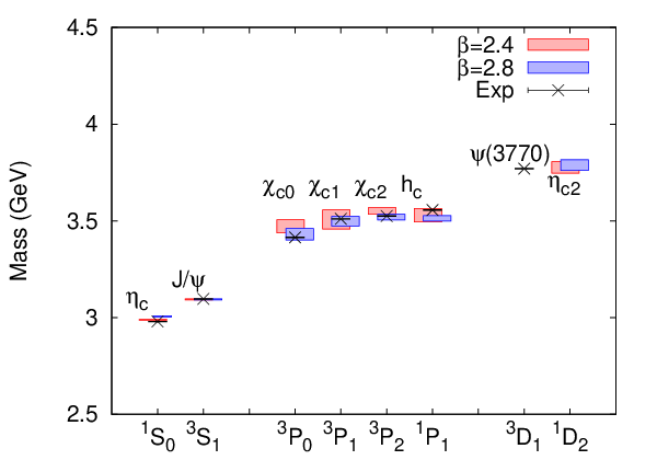
The whole spectrum of the lowest-lying charmonium states we extracted in this work is illustrated in Fig. 2 and listed in Table 2, where the experimental values are also given for comparison. Since we have only two lattice spacings, we would not carry out a serious extrapolation to the continuum limit, but we show all the results, from which one can see that the effects of the finite lattice artifacts and the quenched approximation are not that important.

Refer to caption
Figure 1: The 2−⁣+2^{-+} effective masses of F−FF-F, D​D−FDD-F, F−QF-Q and D​D−QDD-Q correlators at β=2.8\beta=2.8 are plotted for illustration. F−FF-F and F−QF-Q effective masses lie on each other and saturate to the same plateau with the best-fit mass M=4.43​(8)​GeVM=4.43(8)\,{\rm GeV} (indicated by the red line with the jackknife error band). The D​D−QDD-Q effective mass has a plateau at M=3.79​(3)M=3.79(3) ( blue line with the jackknife error band ). In contrast, D​D−FDD-F effective mass does not show perfect plateau, but it evolves gradually from the upper plateau to the lower.
Table 2: Listed here are the masses of the lowest-lying charmoinum states extracted from the two lattices (β=2.4\beta=2.4 and β=2.8\beta=2.8) in this work. The experimental results [5] and the nonrelativistic quark model predictions [19] are also given for comparison.
meson JP​CJ^{PC} M⁡(2.4)M(2.4) M⁡(2.8)M(2.8) Expt. QM
ηc​(S01)\eta_{c}({}^{1}S_{0}) 0−⁣+0^{-+} 2.989(2) 3.007(3) 2.981 2.982
J/ψ⁡(S13)J/\psi({}^{3}S_{1}) 1−⁣−1^{--} 3.094(3) 3.094(3) 3.097 3.090
hc​(P01)h_{c}({}^{1}P_{0}) 1+⁣−1^{+-} 3.530(35) 3.513(14) 3.526 3.516
χc​0​(P03)\chi_{c0}({}^{3}P_{0}) 0+⁣+0^{++} 3.472(34) 3.431(30) 3.415 3.424
χc​1​(P13)\chi_{c1}({}^{3}P_{1}) 1+⁣+1^{++} 3.508(50) 3.499(25) 3.511 3.505
χc​2​(P23)\chi_{c2}({}^{3}P_{2}) 2+⁣+2^{++} 3.552(17) 3.520(15) 3.556 3.556
ψ′′​(D13)\psi^{\prime\prime}({}^{3}D_{1}) 1−⁣−1^{--} - - 3.770 3.785
ηc​2​(D21)\eta_{c2}({}^{1}D_{2}) 2−⁣+2^{-+} 3.777(30) 3.789(28) - 3.799

The goal of the spectroscopy study in this work is twofold. First, the physical spectrum of experimentally established charmonium states can be well reproduced in our formalism. This gives us confidence in our prediciton of the ηc​2\eta_{c2} mass. Second, the practical study finds that the D​DDD-type operator is preferable for producing the 2−⁣+2^{-+} charmonium. Therefore, in the study of its radiative transition, we choose the D​DDD-type operator for ηc​2\eta_{c2} in the calculation of the related three-point functions.
Refer to caption
Figure 2: 1​S1S, 1​P1P, and 1​D1D charmonium spectrum. The red boxes illustrate the results for β=2.4\beta=2.4, and the blue ones for β=2.8\beta=2.8. The experimental value are also plotted with points for comparison.

III.2 Renormalization of the vector current

In the quenched approximation, since there are no sea quarks, the electromagnetic current contributing to the radiative transitions of charmonia involves only the charm quark, say, jem​(x)=Qc​jμ​(x)j_{\rm em}(x)=Q_{c}j^{\mu}(x) with jμ​(x)=c¯​γμ​c​(x)j^{\mu}(x)=\bar{c}\gamma_{\mu}c(x), which is the one we adopt in this study. It is a conserved vector current and need not be renormalized in the continuum. However, on a finite lattice, it is not conserved anymore due to the lattice artifact and receives a multiplicative renormalization factor ZV​(as)Z_{V}(a_{s}). Following the scheme proposed by Ref. [33], ZV​(as)Z_{V}(a_{s}) is extracted using the ratio of the ηc\eta_{c} two-point function and the related three-point function evaluated at Q2=0Q^{2}=0,

ZV(μ)​(t)=pμE⁡(p→)​12​Γηc(2)​(p→,tf=nt2)Γ(3),μ​(p→,p→,nt2,t),Z^{(\mu)}_{V}(t)=\frac{p^{\mu}}{E(\vec{p})}\frac{\frac{1}{2}\Gamma^{(2)}_{\eta_{c}}(\vec{p};t_{f}=\frac{n_{t}}{2})}{\Gamma^{(3),\mu}(\vec{p},\vec{p},\frac{n_{t}}{2},t)},

where the factor 1/21/2 accounts for the effect of the temporal periodic boundary condition, and the superscript μ\mu of ZV​(as)Z_{V}(a_{s}) is used to differentiate the temporal component from the spatial ones, since they are not necessarily the same due to the anisotropic lattices we use. Figure 3 plots ZV(μ)​(t)Z^{(\mu)}_{V}(t) with respect to tt for the two lattices. ZVZ_{V}’s are extracted from the plateaus and the values are listed in Table 3. Obviously, the spatial components ZV(s)​(a)Z_{V}^{(s)}(a) deviate from the temporal ones by a few percent. This deviation can be attributed to the imperfect tuning of the bare velocity in the fermion action. In this work, only ZV(s)Z_{V}^{(s)}’s enter the calculation since only the spatial components of the vector current are involved in the extraction of the form factors.

Table 3: The renormalization constants ZV(s)Z_{V}^{(s)} and ZV(t)Z_{V}^{(t)} of the spatial and temporal components of the vector current for β=2.4\beta=2.4 and β=2.8\beta=2.8 lattices. Two momentum modes, (0,0,0) and (1,0,0)(1,0,0), are used for the derivation.
β\beta ZV(t)​(0,0,0)Z_{V}^{(t)}(0,0,0) ZV(t)​(1,0,0)Z_{V}^{(t)}(1,0,0) ZV(s)​(1,0,0)Z_{V}^{(s)}(1,0,0)
2.42.4 1.288​(5)1.288(5) 1.299​(11)1.299(11) 1.388​(15)1.388(15)
2.82.8 1.155​(3)1.155(3) 1.159​(3)1.159(3) 1.110​(7)1.110(7)
Refer to caption
Refer to caption
Figure 3: The renormalization constant ZVZ_{V} of the vector current. The upper panel is for β=2.4\beta=2.4 and the lower one for β=2.8\beta=2.8. The dots are the simulation data with jackknife errors, and the lines show the fit results.

III.3 Three-point functions and form factors

With the prescriptions discussed above, we now give a brief description of the calculation of the three-point functions. In practice, we use local sink and source operators for the initial and the final states, and insert the vector current jμ​(x)=c¯​γμ​c​(x)j^{\mu}(x)=\bar{c}\gamma^{\mu}c(x) only on the quark line. (The current insertion on the antiquark line is numerically equivalent and is taken into consideration by multiplying by a factor of 2 in the final result.) The three-point functions contributed by the connected diagrams (disconnected diagrams are neglected) are calculated by using the standard sequential source technique. (One can refer to Refs.[33, 34] for the details.) In order to increase the statistics, we repeat the same calculations TT times (where TT is the temporal lattice size) by setting a point source on a different time slice each time. With the related two-point functions calculated accordingly, a straightforward way to extract the interested matrix elements ⟨f⁡(p′→,rf)|jμ​(0)|i⁡(p→,ri)⟩\langle f(\vec{p^{\prime}},r_{f})|j^{\mu}(0)|i(\vec{p},r_{i})\rangle is to fit the three-point function and two-point function simultaneously according to Eq. (5) and Eq. (6). However, it is known that the excited states contribute much to two-point and three-point functions when the time ranges tt and tf−tt_{f}-t are not large enough. This situation is more serious for local operators, so it is not trivial to isolate the contribution of ground states. A way around this is to employ the ratios of correlation functions, which can suppress the contribution of excited states substantially. For this purpose, we introduce the functions Rμ​(t)R^{\mu}(t),

Rμ(t)=Γ(3)(pf→,q→,tf,t)×\displaystyle R^{\mu}(t)=\Gamma^{(3)}(\vec{p_{f}},\vec{q},t_{f},t)\times
2​Ei​Γi(2)​(pi→,tf−t)Γi(2)​(pi→,t)​Γi(2)​(pi→,tf)​2​Ef​Γf(2)​(pf→,t)Γf(2)​(pf→,tf−t)​Γf(2)​(pf→,tf),\displaystyle\sqrt{\frac{2E_{i}\Gamma^{(2)}_{i}(\vec{p_{i}},t_{f}-t)}{\Gamma^{(2)}_{i}(\vec{p_{i}},t)\Gamma^{(2)}_{i}(\vec{p_{i}},t_{f})}}\sqrt{\frac{2E_{f}\Gamma^{(2)}_{f}(\vec{p_{f}},t)}{\Gamma^{(2)}_{f}(\vec{p_{f}},t_{f}-t)\Gamma^{(2)}_{f}(\vec{p_{f}},t_{f})}},

which should be insensitive to the variation of tt in a time window, so that the desired matrix element ⟨f⁡(p→f,rf)|​jμ​(0)|ψ⁡|i⁡(p→i,ri)⟩\langle f(\vec{p}_{f},r_{f})|j^{\mu}(0)|\psi|i(\vec{p}_{i},r_{i})\rangle can be extracted from the plateau.

In the data analysis, we divide the 1000 configurations into 100 bins and use each bin average as an independent measurement. For the resultant 100 bins, we use the one-eliminating jackknife method. Since the energies Ei,fE_{i,f} can be determined very precisely from the two-point functions, they are treated as known parameters in the above equation. Practically, Rμ​(t)R^{\mu}(t) is fitted by the function

Rμ​(t)=⟨f⁡(p→f,rf)​|jμ​(0)|​ψ|i⁡(p→i,ri)⟩+δ​f​(t)R^{\mu}(t)=\langle f(\vec{p}_{f},r_{f})|j^{\mu}(0)|\psi|i(\vec{p}_{i},r_{i})\rangle+\delta f(t) (10)

where the additional term δ​f​(t)=a​e−δ​m​t\delta f(t)=ae^{-\delta mt} accounts for the residual contribution of excited states. Thus we can obtain a jackknife ensemble of the matrix elements. The second step of data analysis is to extract the form factors that enter the calculation of decay widths. Since these matrix elements can be expressed in terms of form factors through the multipole decomposition,

⟨f⁡(p→f,rf)|jμ​(0)|i⁡(p→i,ri)⟩=∑kαkμ​(pi,pf)​F^k​(Q2),\langle f(\vec{p}_{f},r_{f})|j^{\mu}(0)|i(\vec{p}_{i},r_{i})\rangle=\sum_{k}\alpha_{k}^{\mu}(p_{i},p_{f})\hat{F}_{k}(Q^{2}), (11)

and αkμ​(pi,pf)\alpha^{\mu}_{k}(p_{i},p_{f}) are theoretically known kinematic functions, the form factors Fk^​(Q2)\hat{F_{k}}(Q^{2}) can then be derived straightforwardly. Taking into consideration the contribution of the current insertion on the antiquark line, the electric charge of the charm quark Qc=2/3Q_{c}=2/3, and the renormalization constant of the spatial components of the current operator ZV(s)Z_{V}^{(s)}, Fk^\hat{F_{k}} is related to FkF_{k} of Eq. (7) as

Fk​(Q2)=2×23​e×ZV(s)​F^k​(Q2).F_{k}(Q^{2})=2\times\frac{2}{3}e\times Z_{V}^{(s)}\hat{F}_{k}(Q^{2}). (12)

With this in mind, in the following context, we omit the hat of F^\hat{F} and insert ZV(s)Z_{V}^{(s)} implicitly in possible expressions.

In order to take good care of the correlation between the form factors, we carry out correlated minimal χ2\chi^{2} fits with the jackknife covariance matrix built from the jackknife ensemble of the matrix elements. On the other hand, for a specific Q2Q^{2}, there may be several symmetric copies of the matrix elements with the same value of αkμ\alpha_{k}^{\mu}. These copies are averaged over to increase statistics.

In the following subsections, we present first the calculation of the process χc​2→γ​J/ψ\chi_{c2}\rightarrow\gamma J/\psi to see how precisely the form factors- and thereby the transition width- can be derived, and then the results of ηc​2→γ​ψ\eta_{c2}\rightarrow\gamma\psi.

III.4 χc​2→γ​J/ψ\chi_{c2}\rightarrow\gamma J/\psi transition

The Minkowski space-time matrix elements for this transition can be expressed in terms of form factors as follows:

⟨V⁡(p→V,λV)|jμ​(0)|T⁡(p→T,λT)⟩=α1μ​E1​(Q2)\displaystyle\langle V(\vec{p}_{V},\lambda_{V})|j^{\mu}(0)|T(\vec{p}_{T},\lambda_{T})\rangle=\alpha_{1}^{\mu}E_{1}(Q^{2})
+α2μ​M2​(Q2)+α3μ​E3​(Q2)+α4μ​C1​(Q2)+α5μ​C2​(Q2)\displaystyle+\alpha_{2}^{\mu}M_{2}(Q^{2})+\alpha_{3}^{\mu}E_{3}(Q^{2})+\alpha_{4}^{\mu}C_{1}(Q^{2})+\alpha_{5}^{\mu}C_{2}(Q^{2})

where VV stands for the 1−⁣−1^{--} vector meson J/ψJ/\psi, TT stands for the 2+⁣+2^{++} tensor χc​2\chi_{c2}, and αiμ\alpha_{i}^{\mu} are Lorentz covariant kinematic functions of pVp_{V} and pTp_{T} (and specific polarizations of VV and TT), whose explicit expressions are tedious and omitted here. Although a J=2J=2 representation of the rotational symmetry in the continuum breaks into the EE and T2T_{2} irreducible representations (irreps) of the lattice spatial symmetry group OO, we find that this breaking effect is small in our work, as is manifested by the near degeneracy of the masses and spectral weights of the ground states in these two irreps when we study the relevant two-point functions. Thus, we assume that the rotation symmetry breaking is also negligible for the related matrix elements, and we carry out the multipole decomposition on the basis of E​⨁T2E\bigoplus T_{2}, which is equivalent to the J=2J=2 basis up to an orthogonal transformation. One can find the detailed decomposition procedure in Appendix A and may also refer to Refs. [33, 35]. In the practical study, we set TT to be at rest and let VV move with different spatial momenta p→=2​π​n→/L\vec{p}=2\pi\vec{n}/L. The 27 momentum modes of n→=(n1,n2,n3)\vec{n}=(n_{1},n_{2},n_{3}) ranging from (0,0,0)(0,0,0) to (2,2,2)(2,2,2) are calculated for VV.

Refer to caption
Refer to caption
Figure 4: The extracted form factors E1​(Q2)E_{1}(Q^{2}), M2​(Q2)M_{2}(Q^{2}), and E3​(Q2)E_{3}(Q^{2}) are plotted versus Q2Q^{2} for the two lattices of β=2.4\beta=2.4 (the upper panel) and β=2.8\beta=2.8 (the lower panel), respectively, where the points are the simulation data, the line the fit function, and the error bands the jackknife ones. The PDG values of E1​(0)E_{1}(0) and M2​(0)M_{2}(0) are also plotted for comparison.

The transition width of χc​2→γ​J/ψ\chi_{c2}\rightarrow\gamma J/\psi for an on-shell photon (Q2=0Q^{2}=0) involves only the form factors E1​(0)E_{1}(0), M2​(0)M_{2}(0) and E3​(0)E_{3}(0), or explicitly,

Γ⁡(χc​2→γ​J/ψ)=16​α​|k→|45​Mχc​22​(|E1​(0)|2+|M2​(0)|2+|E3​(0)|2)\Gamma(\chi_{c2}\rightarrow\gamma J/\psi)=\frac{16\alpha|\vec{k}|}{45M^{2}_{\chi_{c2}}}(|E_{1}(0)|^{2}+|M_{2}(0)|^{2}+|E_{3}(0)|^{2}) (14)

where |q→|=(Mχc​22−MJ/ψ2)/2​Mχc​2|\vec{q}|=(M_{\chi_{c2}}^{2}-M_{J/\psi}^{2})/2M_{\chi_{c2}} is the decaying energy of the photon, and α=e2/(4​π)\alpha=e^{2}/(4\pi) is the fine structure constant. Since our simulation data are obtained at Q2≠0Q^{2}\neq 0, these on-shell form factors should be interpolated to Q2=0Q^{2}=0. In doing this, we adopt the fitting functional form inspired by the nonrelativistic quark model [33],

Fk​(Q2)=Fk​(0)​(1+λk​Q2)​e−Q216​βk2F_{k}(Q^{2})=F_{k}(0)(1+\lambda_{k}Q^{2})e^{-\frac{Q^{2}}{16\beta_{k}^{2}}} (15)

which has been applied successfully in previous works. Here Fk​(0)F_{k}(0), λk\lambda_{k}, and βk\beta_{k} are the parameters to be fitted though a correlated χ2\chi^{2} fitting procedure where the covariance matrix is constructed using the one-eliminating jackknife method. Plotted in Fig. 4 are the extracted form factors E1​(Q2)E_{1}(Q^{2}), M2​(Q2)M_{2}(Q^{2}), and E3​(Q2)E_{3}(Q^{2}) versus Q2Q^{2} for the two lattices of β=2.4\beta=2.4 (the upper panel) and β=2.8\beta=2.8 (the lower panel). The data points are the simulation results, and the lines are the fit function with the jackknife error bands. One can find that the data are very precise owing to the high statistics, and the fit errors are also very small. We also carry out a simple polynomial fit with respect to Q2Q^{2}, Fk​(Q2)=Fk​(0)+c1​Q2+c2​Q4F_{k}(Q^{2})=F_{k}(0)+c_{1}Q^{2}+c_{2}Q^{4}, and get consistent results within errors. Table 4 lists the results of the interpolation, where the continuum limit extrapolation is also given. It is seen that the electric dipole (E1E_{1}) contribution is dominant in the transition χc​2→γ​J/ψ\chi_{c2}\rightarrow\gamma J/\psi, while the contribution of the magnetic quadrupole (M2M_{2}) is drastically suppressed, as depicted by the ratio

a2=M2​(0)E1​(0)2+M2​(0)2+E3​(0)2,a_{2}=\frac{M_{2}(0)}{\sqrt{E_{1}(0)^{2}+M_{2}(0)^{2}+E_{3}(0)^{2}}}, (16)

for which we get a result a2=−0.107​(3)a_{2}=-0.107(3) for β=2.4\beta=2.4 and a2=−0.082​(7)a_{2}=-0.082(7) for β=2.8\beta=2.8. After a linear extrapolation in as2a_{s}^{2}, we get the value in the continuum limit a2=−0.067​(7)a_{2}=-0.067(7), which is consistent with the PDG data, where a2=−0.100±0.015a_{2}=-0.100\pm 0.015 [5]. The contribution of the electric octupole E3E_{3} is far smaller. For the ratio

a3=E3​(0)E1​(0)2+M2​(0)2+E3​(0)2,a_{3}=\frac{E_{3}(0)}{\sqrt{E_{1}(0)^{2}+M_{2}(0)^{2}+E_{3}(0)^{2}}}, (17)

we obtain a3=0.007​(2)a_{3}=0.007(2) for β=2.4\beta=2.4, a3=0.003​(4)a_{3}=0.003(4) for β=2.8\beta=2.8, and the continuum limit a3=−0.003​(6)a_{3}=-0.003(6), which are also compatible with the PDG data a3=0.016±0.013a_{3}=0.016\pm 0.013 [5]. If we focus on E1E_{1}, we get the fitting parameters β1\beta_{1} and λ1\lambda_{1},

β1\displaystyle\beta_{1} =\displaystyle= 0.431​(5)​GeV\displaystyle 0.431(5)\,{\rm GeV}
λ1\displaystyle\lambda_{1} =\displaystyle= −0.285​(2)​GeV−2\displaystyle-0.285(2)\,{\rm GeV}^{-2} (18)

for β=2.4\beta=2.4 and

β1\displaystyle\beta_{1} =\displaystyle= 0.395​(4)​GeV\displaystyle 0.395(4)\,{\rm GeV}
λ1\displaystyle\lambda_{1} =\displaystyle= −0.336​(3)​GeV−2\displaystyle-0.336(3)\,{\rm GeV}^{-2} (19)

for β=2.8\beta=2.8.

Table 4: Listed here are the results of the interpolated form factors E1​(0)E_{1}(0), M2​(0)M_{2}(0), and E3​(0)E_{3}(0), as well as the transition widths. The continuum limits are also given. All the results are in physical units. The widths can be compared with the PDG data Γ=380​(30)​keV\Gamma=380(30)\,{\rm keV} [5].
β\beta E1​(GeV)E_{1}(\textrm{GeV}) M2​(GeV)M_{2}(\textrm{GeV}) E3​(GeV)E_{3}(\textrm{GeV}) Γ⁡(keV)\Gamma(\textrm{keV})
2.42.4 2.04​(2)2.04(2) −0.218​(4)-0.218(4) 0.014​(3)0.014(3) 347±20347\pm 20
2.82.8 2.08​(2)2.08(2) −0.171​(10)-0.171(10) 0.005​(8)0.005(8) 352±11352\pm 11
Cont. 2.11​(2)2.11(2) −0.141​(15)-0.141(15) −0.007​(12)-0.007(12) 361±9361\pm 9

Using the interpolated form factors Fk​(0)F_{k}(0) and taking the fine structure constant α=1/137\alpha=1/137, the transition width can be calculated directly. As shown in Table 4, the partial decay width of Γ⁡(χc​2→J/ψ​γ)\Gamma(\chi_{c2}\to J/\psi\ \gamma) is predicted to be 347±20347\pm 20 keV or 352±11352\pm 11 keV for the two lattices, respectively. The continuum extrapolation gives Γ=361±9​keV\Gamma=361\pm 9\,{\rm keV}. All these results can be compared with the PDG average of 380​(30)​keV380(30)\,{\rm keV}. The agreement with experimental data of the χc​2→J/ψ​γ\chi_{c2}\to J/\psi\ \gamma transition indicates that our method for the χc​2→J/ψ\chi_{c2}\rightarrow J/\psi transition is reliable. Then we can turn to transition the ηc​2→γ​J/ψ\eta_{c2}\rightarrow\gamma J/\psi.

III.5 ηc​2→J/ψ​γ\eta_{c2}\to J/\psi\gamma transition

The general Lorentz decomposition of the Minkowski matrix elements responsible for the transition ηc​2→γ​J/ψ\eta_{c2}\to\gamma J/\psi can be expressed as

⟨V⁡(p→V,λV)|jμ​(Q2)|T⁡(p→T,λT)⟩=a⁡(Q2)​Aμ\displaystyle\langle V(\vec{p}_{V},\lambda_{V})|j^{\mu}(Q^{2})|T(\vec{p}_{T},\lambda_{T})\rangle={a(Q^{2})}A^{\mu}
+b⁡(Q2)​Bμ+c⁡(Q2)​Cμ+d⁡(Q2)​Dμ+e⁡(Q2)​Eμ\displaystyle+{b(Q^{2})}B^{\mu}+{c(Q^{2})}C^{\mu}+{d(Q^{2})}D^{\mu}+{e(Q^{2})}E^{\mu} (20)

where TT stands now for the tensor meson ηc​2\eta_{c2}; a⁡(Q2)a(Q^{2}), b⁡(Q2)b(Q^{2}), c⁡(Q2)c(Q^{2}), d⁡(Q2)d(Q^{2}), and e⁡(Q2)e(Q^{2}) are Lorentz-invariant scalar functions of Q2Q^{2}, and AμA^{\mu}, BμB^{\mu}, CμC^{\mu}, DμD^{\mu} are kinematic functions whose explicit expressions can be found in Appendix B. With the multipole decomposition, the matrix elements can be also expressed in terms of form factors M1M_{1}, E2E_{2}, M3M_{3}, and C2C_{2}:

⟨V⁡(p→V,λV)|jμ​(0)|T⁡(p→T,λT)⟩=i​α1μ​M1​(Q2)\displaystyle\langle V(\vec{p}_{V},\lambda_{V})|j^{\mu}(0)|T(\vec{p}_{T},\lambda_{T})\rangle=i\alpha_{1}^{\mu}{\ M_{1}(Q^{2})}
+i​α2μ​E2​(Q2)+i​α3μ​M3​(Q2)−i​α4μ​C2​(Q2)\displaystyle+i\alpha_{2}^{\mu}{\ E_{2}(Q^{2})}+i\alpha_{3}^{\mu}{\ M_{3}(Q^{2})}-i\alpha_{4}^{\mu}{\ C_{2}(Q^{2})} (21)

where αiμ\alpha_{i}^{\mu} are also kinematic functions which can be expressed in terms of the kinematic functions in Eq. (20). (See Appendix B.) With real photons in the transition ηc​2→γ​J/ψ\eta_{c2}\to\gamma J/\psi, only three multipoles are contributing: the magnetic dipole (M1M_{1}), the electric quadrupole (E2E_{2}), and M3M_{3}. The transition width is written as

Γ⁡(ηc​2→γ​J/ψ)=16​α​|q→|45​Mηc​22​(|M1​(0)|2+|E2​(0)|2+|M3​(0)|2).\Gamma(\eta_{c2}\rightarrow\gamma J/\psi)=\frac{16\alpha|\vec{q}|}{45M^{2}_{\eta_{c2}}}(|M_{1}(0)|^{2}+|E_{2}(0)|^{2}+|M_{3}(0)|^{2}). (22)

Since they are calculated at Q2≠0Q^{2}\neq 0, the multipole amplitudes should be interpolated to Q2=0Q^{2}=0. The form factor C2​(Q2)C_{2}(Q^{2}) corresponds to the emission of longitudinal photons and does not contribute at Q2=0Q^{2}=0. In extracting the amplitudes, we take the standard procedure as described in Sec. II. The three-point functions are calculated by setting the tensor at rest and making the vector moving. In analogy with the 2+⁣+2^{++} case, the effect of rotational symmetry breaking between T2T_{2} irreps and EE irreps is found to be small in this case and is neglected in the data analysis. The form factors M1​(Q2)M_{1}(Q^{2}), E2​(Q2)E_{2}(Q^{2}), and M3​(Q2)M_{3}(Q^{2}) with various Q2Q^{2} are extracted jointly by a correlated fitting with a one-eliminating jackknife covariance matrix, and the results are illustrated in Fig. 5 as data points with jackknife errors. In the following discussion, we will focus on the interpolation procedure. What is interesting is the relation between the two sets of form factors. We should first mention that the form factors, given the fact that they are functions of Q2Q^{2}, can also be written in terms of another Lorentz invariant variable, Ω\Omega:

Ω\displaystyle\Omega ≡\displaystyle\equiv (pV⋅pT)2−mV2​mT2\displaystyle(p_{V}\cdot p_{T})^{2}-m_{V}^{2}m_{T}^{2} (23)
=\displaystyle= 14​[(mV+mT)2+Q2]​[(mV−mT)2+Q2].\displaystyle\frac{1}{4}[(m_{V}+m_{T})^{2}+Q^{2}][(m_{V}-m_{T})^{2}+Q^{2}].

Thus the two sets of the form factors are related to each other as follows,

M1​(Ω)\displaystyle M_{1}(\Omega) =\displaystyle= iΩmT[512(amV+amT−2cmT)+2​a​mV−3​c​mT−4​d​mV2​mT+6​e​mV​mT24​15(ΩmV2​mT2)\displaystyle i\frac{\sqrt{\Omega}}{m_{T}}\left[\sqrt{\frac{5}{12}}\left(a\ m_{V}+a\ m_{T}-2c\ m_{T}\right)+\frac{2a\ m_{V}-3c\ m_{T}-4d\ m_{V}^{2}m_{T}+6e\ m_{V}m_{T}^{2}}{4\sqrt{15}}\left(\frac{\Omega}{m_{V}^{2}m_{T}^{2}}\right)\right.
+−2​a​mV+3​c​mT16​15(ΩmT2​mV2)2+O((ΩmT2​mV2)3)],\displaystyle+\left.\frac{-2a\ m_{V}+3c\ m_{T}}{16\sqrt{15}}\left(\frac{\Omega}{m_{T}^{2}m_{V}^{2}}\right)^{2}+O\left(\left(\frac{\Omega}{m_{T}^{2}m_{V}^{2}}\right)^{3}\right)\right],
E2​(Ω)\displaystyle E_{2}(\Omega) =\displaystyle= iΩmT[−34(amT−amV)+2​a​mV−c​mT−4​d​mV2​mT+2​e​mV​mT24​3(ΩmV2​mT2)\displaystyle i\frac{\sqrt{\Omega}}{m_{T}}\left[-\sqrt{\frac{3}{4}}\left(a\ m_{T}-a\ m_{V}\right)+\frac{2a\ m_{V}-c\ m_{T}-4d\ m_{V}^{2}m_{T}+2e\ m_{V}m_{T}^{2}}{4\sqrt{3}}\left(\frac{\Omega}{m_{V}^{2}m_{T}^{2}}\right)\right.
+−2​a​mV+c​mT16​3(ΩmT2​mV2)2+O((ΩmT2​mV2)3)],\displaystyle+\left.\frac{-2a\ m_{V}+c\ m_{T}}{16\sqrt{3}}\left(\frac{\Omega}{m_{T}^{2}m_{V}^{2}}\right)^{2}+O\left(\left(\frac{\Omega}{m_{T}^{2}m_{V}^{2}}\right)^{3}\right)\right],
M3​(Ω)\displaystyle M_{3}(\Omega) =\displaystyle= iΩmT[−−a​mV−c​mT+2​d​mV2​mT+2​e​mV​mT215(ΩmV2​mT2)−a​mV+c​mT4​15(ΩmT2​mV2)2\displaystyle i\frac{\sqrt{\Omega}}{m_{T}}\left[-\frac{-a\ m_{V}-c\ m_{T}+2d\ m_{V}^{2}m_{T}+2e\ m_{V}m_{T}^{2}}{\sqrt{15}}\left(\frac{\Omega}{m_{V}^{2}m_{T}^{2}}\right)-\frac{a\ m_{V}+c\ m_{T}}{4\sqrt{15}}\left(\frac{\Omega}{m_{T}^{2}m_{V}^{2}}\right)^{2}\right. (24)
+O((ΩmT2​mV2)3)].\displaystyle+\left.O\left(\left(\frac{\Omega}{m_{T}^{2}m_{V}^{2}}\right)^{3}\right)\right].

It is seen that each multipole form factor can be expressed as a series of Ω/(mV2​mT2)\Omega/(m_{V}^{2}m_{T}^{2}) with a prefactor Ω/mT\sqrt{\Omega}/m_{T}. In the rest frame of TT (as is the case in our calculation), the expression of Ω\Omega is simplified as Ω=(mT​|p→V|)2\Omega=(m_{T}|\vec{p}_{V}|)^{2}, such that Ω/(mV2​mT2)=v2\Omega/(m_{V}^{2}m_{T}^{2})=v^{2}, with v=|p→V|/mVv=|\vec{p}_{V}|/m_{V} being the spatial velocity of VV. The convergence of the series in vv is guaranteed if the form factors aa, bb, cc, dd, ee are not singular in Q2Q^{2}, since v<1v<1 (For our calculation, the largest value of vv is approximately 0.50.5). So, for the decaying TT at rest, we have the simplified expression of the form factors M1M_{1}, E2E_{2}, and M3M_{3}:

M1\displaystyle M_{1} =\displaystyle= |p→V|​(A1​(Q2)+B1​(Q2)​v2+C1​(Q2)​v4+O⁡(v6))\displaystyle|\vec{p}_{V}|(A_{1}(Q^{2})+B_{1}(Q^{2})v^{2}+C_{1}(Q^{2})v^{4}+O(v^{6}))
E2\displaystyle E_{2} =\displaystyle= |p→V|​(A2​(Q2)+B2​(Q2)​v2+C2​(Q2)​v4+O⁡(v6))\displaystyle|\vec{p}_{V}|(A_{2}(Q^{2})+B_{2}(Q^{2})v^{2}+C_{2}(Q^{2})v^{4}+O(v^{6}))
M3\displaystyle M_{3} =\displaystyle= |p→V|​(B3​(Q2)​v2+C3​(Q2)​v4+O⁡(v6)).\displaystyle|\vec{p}_{V}|(B_{3}(Q^{2})v^{2}+C_{3}(Q^{2})v^{4}+O(v^{6})). (25)

With these expressions, the following information can be inferred: (i) The desired |p→V||\vec{p}_{V}| prefactor accounting for the PP-wave decay of ηc​2→γ​J/ψ\eta_{c2}\to\gamma J/\psi is explicitly derived. (ii) The leading contribution to M1M_{1} and E2E_{2} is of order O⁡(1)O(1), while that of M3M_{3} is of order O⁡(v2)O(v^{2}). For the case of this study, since vmax∼0.5v_{\rm max}\sim 0.5, it is reasonable that the nonsingular Ai,BiA_{i},B_{i} and CiC_{i} can be expanded with respect to vv, such that we can take the following functions to do the interpolation:

Fi​(v)\displaystyle F_{i}(v) =\displaystyle= Av+Bv3+Cv5+O(v6)(Fi→M1,E2)\displaystyle Av+Bv^{3}+Cv^{5}+O(v^{6})(F_{i}\to M_{1},~E_{2})
Fi​(v)\displaystyle F_{i}(v) =\displaystyle= B​v3+C​v5+D​v7+O⁡(v9)​(Fi→M3),\displaystyle Bv^{3}+Cv^{5}+Dv^{7}+O(v^{9})(F_{i}\to M_{3}), (26)

and the on-shell amplitudes M1​(Q2=0)M_{1}(Q^{2}=0), E2​(Q2=0)E_{2}(Q^{2}=0), and M3​(Q2=0)M_{3}(Q^{2}=0) can be reached by Fi​(v0)F_{i}(v_{0}) with v0=(mT2−mV2)/(2​mT​mV)v_{0}=(m_{T}^{2}-m_{V}^{2})/(2m_{T}m_{V}). The extracted form factor and the interpolation are shown in Fig. 5, where the data points are the simulated results with jackknife errors. One can see that at v=0v=0 [corresponding to Q2=−(mT−mV)2∼0.5​GeV2Q^{2}=-(m_{T}-m_{V})^{2}\sim 0.5\,{\rm GeV}^{2}] the form factors M1M_{1}, E2E_{2}, and M3M_{3} are surely consistent with zero. The fits using Eq. (26) are also shown as curves with jackknife error bands. The interpolated values of these form factors at Q2=0Q^{2}=0 for both β=2.4\beta=2.4 and β=2.8\beta=2.8 are listed in Table 5, where the resultant transition widths and the corresponding continuum limits are also given. It is surprising that, for both lattices, the obtained |M3||M_{3}| is unexpectedly large and comparable to M1M_{1}. This may be qualitatively attributed to recoiling effects of the charm quark or charm antiquark by emitting the hard photon with an energy Eγ∼0.6​GeVE_{\gamma}\sim 0.6\,{\rm GeV} in this transition, which may result in large form factors d⁡(Q2)d(Q^{2}) and e⁡(Q2)e(Q^{2}) (see the discussion below). In contrast to the mild dependence of M1M_{1} and M3M_{3} on the lattice spacing, the form factor E2E_{2} is very sensitive to the lattice spacing. The reason for this is unclear and under investigation. Anyway, after a naive continuum extrapolation using the data from the two lattices in this work, we get the continuum results of the form factors as follows:

M1\displaystyle M_{1} =\displaystyle= 0.104​(10)​GeV,\displaystyle 0.104(10)\textrm{GeV},
E2\displaystyle E_{2} =\displaystyle= −0.071​(20)​GeV,\displaystyle-0.071(20)\textrm{GeV},
M3\displaystyle M_{3} =\displaystyle= −0.132​(10)​GeV.\displaystyle-0.132(10)\textrm{GeV}. (27)

Applying these results to Eq. (22), the transition width of ηc​2→γ​J/ψ\eta_{c2}\to\gamma J/\psi is predicted to be

Γ⁡(ηc​2→γ​J/ψ)=3.8±0.9​keV.\Gamma(\eta_{c2}\rightarrow\gamma J/\psi)=3.8\pm 0.9\,{\rm keV}. (28)
Refer to caption
Refer to caption
Figure 5: The ηc​2−J/ψ\eta_{c2}-J/\psi transition form factors M1​(Q2)M_{1}(Q^{2}), E2​(Q2)E_{2}(Q^{2}), and M3​(Q2)M_{3}(Q^{2}) are plotted versus Q2Q^{2} for the two lattices of β=2.4\beta=2.4 (the upper panel) and β=2.8\beta=2.8 (the lower panel), respectively. The points are the simulation data, and the lines illustrate the fit function with jackknife error bands.
Table 5: Listed here are the interpolated values of the form factors M1M_{1}, E2E_{2}, and M3M_{3} at Q2=0Q^{2}=0 for both β=2.4\beta=2.4 and β=2.8\beta=2.8. The resultant transition widths and the corresponding continuum limits are also given.
β\beta M1​(GeV)M_{1}(\textrm{GeV}) E2​(GeV)E_{2}(\textrm{GeV}) M3​(GeV)M_{3}(\textrm{GeV}) Γ⁡(keV)\Gamma(\textrm{keV})
2.42.4 0.133​(13)0.133(13) 0.111​(17)0.111(17) −0.093​(9)-0.093(9) 4.4±0.94.4\pm 0.9
2.82.8 0.115​(11)0.115(11) −0.0007​(14)-0.0007(14) −0.117​(9)-0.117(9) 3.1±0.63.1\pm 0.6
Cont. 0.104​(10)0.104(10) −0.071​(20)-0.071(20) −0.132​(10)-0.132(10) 3.8±0.93.8\pm 0.9

There have also been several phenomenological studies on this transition, one of which is in the framework of the light-front quark model [27], where the on-shell transition amplitude is decomposited as

⟨V⁡(p→V,λV)|jμ​(0)|η2​(p→T,λT)⟩=\displaystyle\langle V(\vec{p}_{V},\lambda_{V})|j^{\mu}(0)|\eta_{2}(\vec{p}_{T},\lambda_{T})\rangle=
[2f1ϵμ​ν​ρ​σpνTpρVϵσβ(p→T,λT)ϵβ∗(p→V,λV)\displaystyle\Big[2f_{1}\epsilon^{\mu\nu\rho\sigma}p^{T}_{\nu}p^{V}_{\rho}\epsilon^{\beta}_{\sigma}(\vec{p}_{T},\lambda_{T})\epsilon^{*}_{\beta}(\vec{p}_{V},\lambda_{V})
+(f2+f3)​ϵμ​ν​ρ​σ​pνT​pρV​ϵσ∗​(p→V,λV)​ϵα​β​(p→T,λT)​pαV​pβV\displaystyle+(f_{2}+f_{3})\epsilon^{\mu\nu\rho\sigma}p^{T}_{\nu}p^{V}_{\rho}\epsilon^{*}_{\sigma}(\vec{p}_{V},\lambda_{V})\epsilon^{\alpha\beta}(\vec{p}_{T},\lambda_{T})p^{V}_{\alpha}p^{V}_{\beta}\
+2f4ϵμ​ν​ρ​σpνTpρVϵσβ(p→T,λT)pβVϵ∗α(p→V,λV)pαT],\displaystyle+2f_{4}\epsilon^{\mu\nu\rho\sigma}p^{T}_{\nu}p^{V}_{\rho}\epsilon^{\beta}_{\sigma}(\vec{p}_{T},\lambda_{T})p^{V}_{\beta}\epsilon^{*\alpha}(\vec{p}_{V},\lambda_{V})p^{T}_{\alpha}\Big], (29)

and the effective couplings are determined to be

f1\displaystyle f_{1} =\displaystyle= −0.0140​(2)​GeV−1,\displaystyle-0.0140(2)\textrm{GeV}^{-1},
f2\displaystyle f_{2} =\displaystyle= 0.146​(3)​GeV−3,\displaystyle 0.146(3)\textrm{GeV}^{-3},
f3\displaystyle f_{3} =\displaystyle= −0.092​(1)​GeV−3,\displaystyle-0.092(1)\textrm{GeV}^{-3},
f4\displaystyle f_{4} =\displaystyle= 0.0180​(1)​GeV−3.\displaystyle 0.0180(1)\textrm{GeV}^{-3}. (30)

Since this decomposition is equivalent to Eq. (20) by the relation

c⁡(0)=2​f1,d⁡(0)=−(f2+f3),e⁡(0)=−2​f4\displaystyle c(0)=2f_{1},\ d(0)=-(f_{2}+f_{3}),\ e(0)=-2f_{4} (31)

[It should be notified that a⁡(Q2)a(Q^{2}) and b⁡(Q2)b(Q^{2}) are equal to zero when Q2=0Q^{2}=0 because they are proportion to C2​(Q2)C_{2}(Q^{2}).], the corresponding multipole amplitudes can be calculated from Eq. (24) as

M1\displaystyle M_{1} =\displaystyle= 0.079​(2)​GeV,\displaystyle 0.079(2)\textrm{GeV},
E2\displaystyle E_{2} =\displaystyle= −0.086​(2)​GeV,\displaystyle-0.086(2)\textrm{GeV},
M3\displaystyle M_{3} =\displaystyle= −0.125​(3)​GeV,\displaystyle-0.125(3)\textrm{GeV}, (32)

which gives a width of Γ\Gamma=3.54(12) keV. Taking into consideration the uncertainty of the choice of parameters such as the charm quark mass mcm_{c} and the wave function parameter, etc., one can find that the lattice results and the LFQM results are surprisingly in excellent agreement. On the other hand, with the values in Eq. (30), we find that the coefficients Bi​(Q2)B_{i}(Q^{2}) of the v2v^{2} term in Eq. (25) are surely much larger than Ai​(Q2)A_{i}(Q^{2}) at Q2=0Q^{2}=0 so as to compensate for the suppression of v2v^{2}. This explains to some extent the fact that the M3M_{3} in this transition competes M1M_{1} and E2E_{2}.

The other phenomenological study [28] applying the nonrelativistic QCD (NRQCD) gives the transition width as

Γ⁡(ηc​2→γ​J/ψ)=8​α​|k→|3675​mc2​(a12+a22+a32)\Gamma(\eta_{c2}\to\gamma J/\psi)=\frac{8\alpha|\vec{k}|^{3}}{675m^{2}_{c}}(a_{1}^{2}+a_{2}^{2}+a_{3}^{2}) (33)

where a1a_{1}, a2a_{2}, and a3a_{3} are equivalent to the standard formfactors M1M_{1}, E2E_{2}, and M3M_{3} up to a constant factor and are calculated explicitly in NRQCD. By comparing this equation with Eq. (14), the factor is approximately 0.33​GeV0.33\,{\rm GeV}, say, Fi≃(0.33​GeV)​aiF_{i}\simeq(0.33\,{\rm GeV})a_{i}. Thus, their work gives the predictions

M1∼0.026−0.045​GeV,E2≃M3≃−0.13​GeV,M_{1}\sim 0.026-0.045\,{\rm GeV},E_{2}\simeq M_{3}\simeq-0.13\,{\rm GeV}, (34)

which are also in reasonable agreement with our results.

IV Conclusion

We calculate in the quenched approximation the mass of JP​C=2−⁣+J^{PC}=2^{-+} charmonium ηc​2\eta_{c2}, as well as its radiative transition width to J/ψJ/\psi. The computations are carried out on two anisotropic lattices with different lattice spacings, such that the lattice artifacts can be controlled to some extent. As a calibration, we calculate first the spectrum of the lowest-lying charmonia, such as 1​S1S and 1​P1P states, and reproduce the physical pattern of the spectrum. In addition, we calculate the transition width of χc​2→γ​J/ψ\chi_{c2}\rightarrow\gamma J/\psi and get the result 361±9​keV361\pm 9\,{\rm keV}, which is in good agreement with the experimental value of 380±30​keV380\pm 30\,{\rm keV}. Both of these facts manifest the small systematic uncertainties due to the quenched approximation and the finite lattice spacings.

There are two states observed in the 2−⁣+2^{-+} channel, with masses 3.80​(3)​GeV3.80(3)\,{\rm GeV} and 4.43​(8)​GeV4.43(8)\,{\rm GeV}. The lower state has a mass similar to that of the well-established ψ⁡(3770)\psi(3770), which is always assigned to be mainly the 1​D131{}^{3}D_{1} charmonium, and therefore can be naturally identified as the conventional 1​D211{}^{1}D_{2} charmonium ηc​2\eta_{c2}. Obviously, it is about 70 MeV lower in mass than X⁡(3872)X(3872), and this difference cannot be attributed to the systematic uncertainties of our work.

As for the transition rate of ηc​2→J/ψ​γ\eta_{c2}\to J/\psi\gamma, we get a small partial width of roughly 3.8(9) keV, which is in agreement with the phenomenological studies. Taking the branch ratio Br⁡(X⁡(3872)→J/ψ​γ)>0.9%​(B​A​B​A​R){\rm Br}(X(3872)\rightarrow J/\psi\gamma)>0.9\%~(BABAR) or 0.6%​(Belle)0.6\%~({\rm Belle}), the full width of X⁡(3872)X(3872) is estimated to be <420−630<420-630 keV, which is smaller than, but not in contradiction with the experimental upper limit ΓX<1.2​MeV\Gamma_{X}<1.2\,{\rm MeV}. Obviously, a reliable calculation of the partial width ηc​2→ψ′​γ\eta_{c2}\to\psi^{\prime}\gamma is also crucial for the D21{}^{1}D_{2} charmonium assignment of X⁡(3872)X(3872), but unfortunately there are difficulties in the unambiguous extraction of excited states on the lattice. However, we can still infer some useful information from the calculation of ηc​2→J/ψ​γ\eta_{c2}\to J/\psi\ \gamma. In the potential quark model, it is known that D21→γ​V{}^{1}D_{2}\to\gamma V is a hindered transition with M1​(0)=0M_{1}(0)=0; therefore, the observed nonzero M1​(0)M_{1}(0) and the appearance of the higher multipoles E2E_{2} and M3M_{3} can be understood as the relativistic correction and the recoil effects of the emission of a hard photon (Eγ∼0.65​GeVE_{\gamma}\sim 0.65\,{\rm GeV} for the final J/ψJ/\psi and Eγ∼0.11​GeVE_{\gamma}\sim 0.11\,{\rm GeV} for ψ′\psi^{\prime}). Intuitively, this kind of effect for the final ψ′\psi^{\prime} can be similar to that for the final J/ψJ/\psi, or even milder; thus, the width of ηc​2→γ​ψ′\eta_{c2}\to\gamma\psi^{\prime} will be suppressed by a kinematic factor of (0.65/0.11)3∼200(0.65/0.11)^{3}\sim 200 when compared with the transition ηc​2→γ​J/ψ\eta_{c2}\to\gamma J/\psi. With this fact in mind, the ηc​2\eta_{c2} assignment of X⁡(3872)X(3872) can be ruled out if BABAR’s observation of Br⁡(X⁡(3872)→γ​ψ′)/Br⁡(X⁡(3872)→γ​J/ψ)=3.4±1.4{\rm Br}(X(3872)\to\gamma\psi^{\prime})/{\rm Br}(X(3872)\to\gamma J/\psi)=3.4\pm 1.4 is confirmed.

ACKNOWLEDGEMENTS

This work was supported in part by the National Science Foundation of China (NSFC) under Grants No. 10835002, No. 11075167, No. 11021092, No. 10975076, and No. 11105153. Y. Chen and C. Liu also thank the support of NSFC and DFG (CRC110).

Appendix A Multipoles decomposition of χc​2↔J/ψ\chi_{c2}\leftrightarrow J/\psi

For the convenience of readers, the details of the multipole decomposition of matrix elements of the electromagnetic current jμ​(0)j^{\mu}(0) between a 1−⁣−1^{--} vector VV state and a 2+⁣+2^{++} tensor state are described here following Ref. [35]. The most general Lorentz-covariant decomposition with PP and CC parity invariance is

⟨V⁡(p→V,λV)|jμ​(0)|T⁡(p→T,λT)⟩=a⁡(Q2)​Aμ+b⁡(Q2)​Bμ\displaystyle\langle V(\vec{p}_{V},\lambda_{V})|j^{\mu}(0)|T(\vec{p}_{T},\lambda_{T})\rangle=a(Q^{2})A^{\mu}+b(Q^{2})B^{\mu}
+c⁡(Q2)​Cμ+dT​(Q2)​DTμ+dV​(Q2)​DVμ\displaystyle~~~~~~+c(Q^{2})C^{\mu}+d_{T}(Q^{2})D_{T}^{\mu}+d_{V}(Q^{2})D_{V}^{\mu}
+fT​(Q2)​FTμ+fV​(Q2)​FVμ\displaystyle~~~~~~+f_{T}(Q^{2})F_{T}^{\mu}+f_{V}(Q^{2})F_{V}^{\mu} (35)

with the definitions

Aμ\displaystyle A^{\mu} ≡\displaystyle\equiv ϵμ​ν​(p→T,λT)​ϵν∗​(p→V,λV);\displaystyle\epsilon^{\mu\nu}(\vec{p}_{T},\lambda_{T})\epsilon^{*}_{\nu}(\vec{p}_{V},\lambda_{V});
Bμ\displaystyle B^{\mu} ≡\displaystyle\equiv ϵμ​ν​(p→T,λT)​pνV​(ϵ∗​(p→V,λV)⋅pT);\displaystyle\epsilon^{\mu\nu}(\vec{p}_{T},\lambda_{T})p^{V}_{\nu}(\epsilon^{*}(\vec{p}_{V},\lambda_{V})\cdot p_{T});
Cμ\displaystyle C^{\mu} ≡\displaystyle\equiv ϵ∗μ​(p→V,λV)​(ϵα​β​(p→T,λT)​pαV​pβV);\displaystyle\epsilon^{*\mu}(\vec{p}_{V},\lambda_{V})(\epsilon^{\alpha\beta}(\vec{p}_{T},\lambda_{T})p^{V}_{\alpha}p^{V}_{\beta});
DTμ\displaystyle D_{T}^{\mu} ≡\displaystyle\equiv pTμ​(ϵα​β​(p→T,λT)​ϵα∗​(p→V,λV)​pβV);\displaystyle p_{T}^{\mu}(\epsilon^{\alpha\beta}(\vec{p}_{T},\lambda_{T})\epsilon^{*}_{\alpha}(\vec{p}_{V},\lambda_{V})p^{V}_{\beta});
DVμ\displaystyle D_{V}^{\mu} ≡\displaystyle\equiv pVμ​(ϵα​β​(p→T,λT)​ϵα∗​(p→V,λV)​pβV);\displaystyle p_{V}^{\mu}(\epsilon^{\alpha\beta}(\vec{p}_{T},\lambda_{T})\epsilon^{*}_{\alpha}(\vec{p}_{V},\lambda_{V})p^{V}_{\beta});
FTμ\displaystyle F_{T}^{\mu} ≡\displaystyle\equiv pTμ​(ϵα​β​(p→T,λT)​pαV​pβV)​(ϵ∗​(p→V,λV)⋅pT);\displaystyle p_{T}^{\mu}(\epsilon^{\alpha\beta}(\vec{p}_{T},\lambda_{T})p^{V}_{\alpha}p^{V}_{\beta})(\epsilon^{*}(\vec{p}_{V},\lambda_{V})\cdot p_{T});
FVμ\displaystyle F_{V}^{\mu} ≡\displaystyle\equiv pVμ​(ϵα​β​(p→T,λT)​pαV​pβV)​(ϵ∗​(p→V,λV)⋅pT).\displaystyle p_{V}^{\mu}(\epsilon^{\alpha\beta}(\vec{p}_{T},\lambda_{T})p^{V}_{\alpha}p^{V}_{\beta})(\epsilon^{*}(\vec{p}_{V},\lambda_{V})\cdot p_{T}).

On the other hand, the matrix elements ⟨V|jμ|T⟩\langle V|j^{\mu}|T\rangle can be also expressed in terms of the helicity amplitudes:

⟨V|jμ|T⟩ϵμ∗(λγ=±)\displaystyle\langle V|j^{\mu}|T\rangle\epsilon^{*}_{\mu}(\lambda_{\gamma}=\pm) =\displaystyle= ∑k2​k+12​J+1[Ek12(1+(−1)kδP)∓Mk12(1−(−1)kδP)]⟨k∓;J′λ±1|Jλ⟩\displaystyle\sum_{k}\sqrt{\frac{2k+1}{2J+1}}\left[E_{k}\tfrac{1}{2}(1+(-1)^{k}\delta P)\mp M_{k}\tfrac{1}{2}(1-(-1)^{k}\delta P)\right]\langle k\mp;J^{\prime}\lambda\pm 1|J\lambda\rangle (37)
⟨V|jμ|T⟩​ϵμ∗​(λγ=0)\displaystyle\langle V|j^{\mu}|T\rangle\epsilon^{*}_{\mu}(\lambda_{\gamma}=0) =\displaystyle= ∑k2​k+12​J+1Ck12(1+(−1)kδP)⟨k0;J′λ|Jλ⟩,\displaystyle\sum_{k}\sqrt{\frac{2k+1}{2J+1}}C_{k}\tfrac{1}{2}(1+(-1)^{k}\delta P)\langle k0;J^{\prime}\lambda|J\lambda\rangle, (38)

where EkE_{k}, MkM_{k}, and CKC_{K} are multipole amplitudes, and δ​P\delta P is the product of the PP parity of the initial (TT) and finial (VV) states, taking the value δ​P=−1\delta P=-1 for the 2+→1−2^{+}\rightarrow 1^{-} transition. These are actually the helicity selection rules. An additional constraint comes from the conservation of the vector current,

⟨V|jμ|T⟩​qμ=∂μ⟨V|jμ|T⟩=0.\langle V|j^{\mu}|T\rangle q_{\mu}=\partial_{\mu}\langle V|j^{\mu}|T\rangle=0. (39)

With the constraints of Eqs. (37, 38, 39), we can solve a⁡(Q2)a(Q^{2}), b⁡(Q2)b(Q^{2}), c⁡(Q2),…c(Q^{2}),\ldots in the rest frame of the initial state with the spatial momentum of the photon parallel to the zz axis. [The polarization vector of the photon takes (1,0,0,1)(1,0,0,1).] Thus, we can get the expressions in terms of Ek​(q2)E_{k}(q^{2}), CK​(Q2)C_{K}(Q^{2}). After that, the general expression of the form factor aa, bb, cc, …\ldots can be obtained by carrying out a general Lorentz transformation. For the case of the 2+→1−2^{+}\rightarrow 1^{-} transition here, Eq. (37) provides three independent equations with respect to the three different helicities of the vector state, and therefore gives the relations between [a⁡(Q2),b⁡(Q2),c⁡(Q2)a(Q^{2}),b(Q^{2}),c(Q^{2})] and E1​(Q2)E_{1}(Q^{2}), M2​(Q2)M_{2}(Q^{2}), E3​(Q2)E_{3}(Q^{2})] as

a\displaystyle a =\displaystyle= E315−M2​3+35​E1,\displaystyle\frac{E_{3}}{\sqrt{15}}-M_{2}{\sqrt{3}}+\sqrt{\frac{3}{5}}E_{1},
b\displaystyle b =\displaystyle= 15​3​Ω(35E1(mTmV−pT.pV)\displaystyle\frac{1}{5\sqrt{3}\Omega}\left(3\sqrt{5}E_{1}(m_{T}m_{V}-p_{T}.p_{V})\right.
+5M2(mImV+pT.pV)\displaystyle+5M_{2}(m_{I}m_{V}+p_{T}.p_{V})
−5E3(4mTmV+pT.pV))\displaystyle-\left.\sqrt{5}E_{3}(4m_{T}m_{V}+p_{T}.p_{V})\right)
c\displaystyle c =\displaystyle= mT2​5​E3+4​M22​3​Ω,\displaystyle m_{T}^{2}\frac{\sqrt{5}E_{3}+4M_{2}}{2\sqrt{3}\Omega}, (40)

with Ω≡(pT⋅pV)2−mT2​mV2\Omega\equiv(p_{T}\cdot p_{V})^{2}-m_{T}^{2}m_{V}^{2}. The constraints from Eqs. (38) and (39) with plus/minus helicity of the vector meson can fix the parameters dVd_{V} and dTd_{T}. Furthermore, fVf_{V} and fTf_{T} can be derived from Eqs. (38) and (39) with zero helicity of the vector meson. As such, the multipole decomposition of the matrix elements ⟨V|jμ|T⟩\langle V|j^{\mu}|T\rangle can be expressed finally as

⟨V⁡(p→V,λV)|jμ​(Q2)|T⁡(p→T,λT)⟩=α1μ​E1​(Q2)\displaystyle\langle V(\vec{p}_{V},\lambda_{V})|j^{\mu}(Q^{2})|T(\vec{p}_{T},\lambda_{T})\rangle=\alpha_{1}^{\mu}E_{1}(Q^{2})
+α2μ​M2​(Q2)+α3μ​E3​(Q2)+α4μ​C1​(Q2)+α5μ​C3​(Q2)\displaystyle+\alpha_{2}^{\mu}M_{2}(Q^{2})+\alpha_{3}^{\mu}E_{3}(Q^{2})+\alpha_{4}^{\mu}C_{1}(Q^{2})+\alpha_{5}^{\mu}C_{3}(Q^{2})

with the functions αiμ\alpha_{i}^{\mu} defined by

α1μ\displaystyle\alpha_{1}^{\mu} =\displaystyle= 35​[−Aμ+mTΩ​(ω~−mV)​Bμ+mTΩ​(ω~​DTμ−mT​DVμ)+mT2Ω2​(ω~−mV)​(−ω~​FTμ+mT​FVμ)]\displaystyle\sqrt{\frac{3}{5}}\Bigg[-A^{\mu}+\frac{m_{T}}{\Omega}(\tilde{\omega}-m_{V})B^{\mu}+\frac{m_{T}}{\Omega}\Big(\tilde{\omega}D_{T}^{\mu}-m_{T}D_{V}^{\mu}\Big)+\frac{m_{T}^{2}}{\Omega^{2}}(\tilde{\omega}-m_{V})\Big(-\tilde{\omega}F_{T}^{\mu}+m_{T}F_{V}^{\mu}\Big)\Bigg]
α2μ\displaystyle\alpha_{2}^{\mu} =\displaystyle= 13[Aμ−mTΩ(ω~+mV)Bμ−2​mT2ΩCμ+mTΩ(−ω~DTμ+mTDVμ)\displaystyle\sqrt{\frac{1}{3}}\Bigg[A^{\mu}-\frac{m_{T}}{\Omega}(\tilde{\omega}+m_{V})B^{\mu}-\frac{2m_{T}^{2}}{\Omega}C^{\mu}+\frac{m_{T}}{\Omega}\Big(-\tilde{\omega}D_{T}^{\mu}+m_{T}D_{V}^{\mu}\Big)
+mT2Ω2((ω~2+ω~mV−2mV2)FTμ+mi(ω~−mV)FVμ)]\displaystyle~~~~~~+\frac{m_{T}^{2}}{\Omega^{2}}\Big((\tilde{\omega}^{2}+\tilde{\omega}m_{V}-2m_{V}^{2})F_{T}^{\mu}+m_{i}(\tilde{\omega}-m_{V})F_{V}^{\mu}\Big)\Bigg]
α3μ\displaystyle\alpha_{3}^{\mu} =\displaystyle= 115[−Aμ+mTΩ(ω~+4mV)Bμ−5​mT22​ΩCμ+mTΩ(ω~DTμ−mTDVμ)\displaystyle\sqrt{\frac{1}{15}}\Bigg[-A^{\mu}+\frac{m_{T}}{\Omega}(\tilde{\omega}+4m_{V})B^{\mu}-\frac{5m_{T}^{2}}{2\Omega}C^{\mu}+\frac{m_{T}}{\Omega}\Big(\tilde{\omega}D_{T}^{\mu}-m_{T}D_{V}^{\mu}\Big)
+mT2Ω2(−(ω~2+4ω~mV+52mV2)FTμ+mi(72ω~+4mV)FVμ)]\displaystyle~~~~~~+\frac{m_{T}^{2}}{\Omega^{2}}\Big(-(\tilde{\omega}^{2}+4\tilde{\omega}m_{V}+\tfrac{5}{2}m_{V}^{2})F_{T}^{\mu}+m_{i}(\tfrac{7}{2}\tilde{\omega}+4m_{V})F_{V}^{\mu}\Big)\Bigg]
α4μ\displaystyle\alpha_{4}^{\mu} =\displaystyle= 35​mTΩ​q2​[(mV2−ω~​mT)​DTμ+(mT2−ω~​mT)​DVμ−mTΩ​(ω~−mV)​((mV2−ω~​mT)​FTμ+(mT2−ω~​mT)​FVμ)]\displaystyle\sqrt{\frac{3}{5}}\frac{m_{T}}{\Omega\sqrt{q^{2}}}\Bigg[(m_{V}^{2}-\tilde{\omega}m_{T})D_{T}^{\mu}+(m_{T}^{2}-\tilde{\omega}m_{T})D_{V}^{\mu}-\frac{m_{T}}{\Omega}\big(\tilde{\omega}-m_{V}\big)\Big((m_{V}^{2}-\tilde{\omega}m_{T})F_{T}^{\mu}+(m_{T}^{2}-\tilde{\omega}m_{T})F_{V}^{\mu}\Big)\Bigg]
α5μ\displaystyle\alpha_{5}^{\mu} =\displaystyle= 25​mTΩ​q2​[(mV2−ω~​mT)​DTμ+(mT2−ω~​mT)​DVμ−mTΩ​(ω~+32​mV)​((mV2−ω~​mT)​FTμ+(mT2−ω~​mT)​FVμ)].\displaystyle\sqrt{\frac{2}{5}}\frac{m_{T}}{\Omega\sqrt{q^{2}}}\Bigg[(m_{V}^{2}-\tilde{\omega}m_{T})D_{T}^{\mu}+(m_{T}^{2}-\tilde{\omega}m_{T})D_{V}^{\mu}-\frac{m_{T}}{\Omega}\big(\tilde{\omega}+\tfrac{3}{2}m_{V}\big)\Big((m_{V}^{2}-\tilde{\omega}m_{T})F_{T}^{\mu}+(m_{T}^{2}-\tilde{\omega}m_{T})F_{V}^{\mu}\Big)\Bigg].

where ω~≡pT.pVmT\tilde{\omega}\equiv\frac{p_{T}.p_{V}}{m_{T}} and ω±≡pT.pV±mV​mT\omega^{\pm}\equiv p_{T}.p_{V}\pm m_{V}m_{T}.

Appendix B Multipoles of ηc​2↔J/ψ\eta_{c2}\leftrightarrow J/\psi

The case of ηc​2→J/ψ\eta_{c2}\rightarrow J/\psi is sightly different from that above. The most general Lorentz-covariant decomposition with PP and CC parity invariance is

⟨V⁡(p→V,λV)|jμ​(0)|η2​(p→T,λT)⟩=a⁡(Q2)​Aμ+b⁡(Q2)​Bμ\displaystyle\langle V(\vec{p}_{V},\lambda_{V})|j^{\mu}(0)|\eta_{2}(\vec{p}_{T},\lambda_{T})\rangle=a(Q^{2})A^{\mu}+b(Q^{2})B^{\mu}
+c⁡(Q2)​Cμ+d⁡(Q2)​Dμ+e⁡(Q2)​Eμ\displaystyle~~~~~~~~+c(Q^{2})C^{\mu}+d(Q^{2})D^{\mu}+e(Q^{2})E^{\mu} (43)

with

Aμ\displaystyle A^{\mu} =\displaystyle= ϵμ​ν​ρ​σ​ϵν∗​(p→V,λV)​pρV​ϵσβ​(p→T,λT)​pβV,\displaystyle\epsilon^{\mu\nu\rho\sigma}\epsilon^{*}_{\nu}(\vec{p}_{V},\lambda_{V})p^{V}_{\rho}\epsilon^{\beta}_{\sigma}(\vec{p}_{T},\lambda_{T})p^{V}_{\beta},
Bμ\displaystyle B^{\mu} =\displaystyle= ϵβ​ν​ρ​σ​pβT​ϵν∗​(p→V,λV)​pρV​ϵσμ​(p→T,λT),\displaystyle\epsilon^{\beta\nu\rho\sigma}p^{T}_{\beta}\epsilon^{*}_{\nu}(\vec{p}_{V},\lambda_{V})p^{V}_{\rho}\epsilon^{\mu}_{\sigma}(\vec{p}_{T},\lambda_{T}),
Cμ\displaystyle C^{\mu} =\displaystyle= ϵμ​ν​ρ​σ​pνT​pρV​ϵσβ​(p→T,λT)​ϵβ∗​(p→V,λV),\displaystyle\epsilon^{\mu\nu\rho\sigma}p^{T}_{\nu}p^{V}_{\rho}\epsilon^{\beta}_{\sigma}(\vec{p}_{T},\lambda_{T})\epsilon^{*}_{\beta}(\vec{p}_{V},\lambda_{V}),\
Dμ\displaystyle D^{\mu} =\displaystyle= ϵμ​ν​ρ​σ​pνV​pρT​ϵσ∗​(p→V,λV)​ϵα​β​(p→T,λT)​pαV​pβV,\displaystyle\epsilon^{\mu\nu\rho\sigma}p^{V}_{\nu}p^{T}_{\rho}\epsilon^{*}_{\sigma}(\vec{p}_{V},\lambda_{V})\epsilon^{\alpha\beta}(\vec{p}_{T},\lambda_{T})p^{V}_{\alpha}p^{V}_{\beta},\
Eμ\displaystyle E^{\mu} =\displaystyle= ϵμ​ν​ρ​σ​pνV​pρT​ϵσβ​(p→T,λT)​pβV​ϵ∗α​(p→V,λV)​pαT.\displaystyle\epsilon^{\mu\nu\rho\sigma}p^{V}_{\nu}p^{T}_{\rho}\epsilon^{\beta}_{\sigma}(\vec{p}_{T},\lambda_{T})p^{V}_{\beta}\epsilon^{*\alpha}(\vec{p}_{V},\lambda_{V})p^{T}_{\alpha}.\ (44)

In fact, there exist another three Lorentz-covariant structures ATA_{T}, EVE_{V}, and ETE_{T}:

EVμ\displaystyle E_{V}^{\mu} =\displaystyle= ϵα​ν​ρ​σ​pαT​ϵβ∗​(p→V,λV)​pρV​ϵσ​β​(p→T,λT)​pβV​pVμ,\displaystyle\epsilon^{\alpha\nu\rho\sigma}p^{T}_{\alpha}\epsilon^{*}_{\beta}(\vec{p}_{V},\lambda_{V})p^{V}_{\rho}\epsilon^{\sigma\beta}(\vec{p}_{T},\lambda_{T})p^{V}_{\beta}p^{\mu}_{V},\
ATμ\displaystyle A_{T}^{\mu} =\displaystyle= ϵμ​ν​ρ​σ​ϵν∗​(p→V,λV)​pρT​ϵσβ​(p→T,λT)​pβV,\displaystyle\epsilon^{\mu\nu\rho\sigma}\epsilon^{*}_{\nu}(\vec{p}_{V},\lambda_{V})p^{T}_{\rho}\epsilon^{\beta}_{\sigma}(\vec{p}_{T},\lambda_{T})p^{V}_{\beta},\
ETμ\displaystyle E_{T}^{\mu} =\displaystyle= ϵα​ν​ρ​σ​pαT​ϵβ∗​(p→V,λV)​pρV​ϵσ​β​(p→T,λT)​pβV​pTμ,\displaystyle\epsilon^{\alpha\nu\rho\sigma}p^{T}_{\alpha}\epsilon^{*}_{\beta}(\vec{p}_{V},\lambda_{V})p^{V}_{\rho}\epsilon^{\sigma\beta}(\vec{p}_{T},\lambda_{T})p^{V}_{\beta}p^{\mu}_{T}, (45)

which, however, are not independent and can be expressed in terms of the functions in Eq. (44):

ATμ\displaystyle A_{T}^{\mu} =\displaystyle= −Bμ−Cμ\displaystyle-B^{\mu}-C^{\mu}
ETμ\displaystyle E_{T}^{\mu} =\displaystyle= mT2​Aμ+pV.pT​Bμ+pV.pT​Cμ+Eμ\displaystyle m_{T}^{2}A^{\mu}+p_{V}.p_{T}B^{\mu}+p_{V}.p_{T}C^{\mu}+E^{\mu}
EVμ\displaystyle E_{V}^{\mu} =\displaystyle= pV⋅pT​Aμ+mV2​Bμ+mV2​Cμ+Dμ.\displaystyle p_{V}\cdot p_{T}A^{\mu}+m_{V}^{2}B^{\mu}+m_{V}^{2}C^{\mu}+D^{\mu}. (46)

So they do not appear in the decomposition. Based on this, one can follow the similar procedure of the case of χc​2→J/ψ\chi_{c2}\rightarrow J/\psi to derive the related multipole decomposition. The constraints of decomposition are similar to Eqs. (37,39) while δ​P=1\delta P=1. Finally, one can get the result

⟨V⁡(p→V,λV)|jμ​(0)|η2​(p→T,λT)⟩=\displaystyle\langle V(\vec{p}_{V},\lambda_{V})|j^{\mu}(0)|\eta_{2}(\vec{p}_{T},\lambda_{T})\rangle=
i​M1​(Q2)5​Ω1/2[−15Cμ+1Ω15Eμ(−mVmT+pT.pV)]\displaystyle\frac{i\ M_{1}(Q^{2})}{5\Omega^{1/2}}\Big[-\sqrt{15}C^{\mu}+\frac{1}{\Omega}\sqrt{15}E^{\mu}(-m_{V}m_{T}+p_{T}.p_{V})\Big]
+i​E2​(Q2)3​Ω1/2[3Cμ+1Ω(23DμmT2−3Eμ(mVmT+pT.pV))]\displaystyle+\frac{i\ E_{2}(Q^{2})}{3\Omega^{1/2}}\Big[\sqrt{3}C^{\mu}+\frac{1}{\Omega}\Big(2\sqrt{3}D^{\mu}m_{T}^{2}-\sqrt{3}E^{\mu}(m_{V}m_{T}+p_{T}.p_{V})\Big)\Big]
+i​M3​(Q2)30​Ω1/2[−215Cμ+1Ω(515DμmT2+215Eμ(4mVmT+pT.pV))]\displaystyle+\frac{i\ M_{3}(Q^{2})}{30\Omega^{1/2}}\Big[-2\sqrt{15}C^{\mu}+\frac{1}{\Omega}\Big(5\sqrt{15}D^{\mu}m_{T}^{2}+2\sqrt{15}E^{\mu}(4m_{V}m_{T}+p_{T}.p_{V})\Big)\Big]
−i​C2​(Q2)q2​Ω1/2[AμmT+BμmT+CμmT+1Ω(DμmT(mT2−pT.pV)+EμmT(mV2−pT.pV))]\displaystyle-\frac{i\ C_{2}(Q^{2})}{\sqrt{q^{2}}\Omega^{1/2}}\Big[A^{\mu}m_{T}+B^{\mu}m_{T}+C^{\mu}m_{T}+\frac{1}{\Omega}\Big(D^{\mu}m_{T}(m_{T}^{2}-p_{T}.p_{V})+E^{\mu}m_{T}(m_{V}^{2}-p_{T}.p_{V})\Big)\Big] (47)

Appendix C Form factor as function of Q2Q^{2} or Ω\Omega

Transition form factors are always expressed as Lorentz scalar functions of the squared momentum transfer, Q2=−q2=−(qi−qf)2Q^{2}=-q^{2}=-(q_{i}-q_{f})^{2}, where pip_{i} and pfp_{f} refer to the four-momenta of the initial and final particles, respectively. However, if one looks into the Lorentz decomposition [Eq. (35)] and the multipole decomposition [Eq. (A)] for the χc​2→J/ψ\chi_{c2}\rightarrow J/\psi transition matrix elements, one can find that the quantity Ω≡(pi.pf)2−mi2mf2\Omega\equiv(p_{i}.p_{f})^{2}-m_{i}^{2}m_{f}^{2}, with pi.pf=(mi2+mf2+Q2)/2p_{i}.p_{f}=(m_{i}^{2}+m_{f}^{2}+Q^{2})/2, is also an interesting Lorentz-invariant kinematic variable. According to Eq. (40), the multipole amplitudes E1E_{1}, M2M_{2}, and E3E_{3} can be reversely expressed in terms of the form factors aa, bb, cc as,

E1​(Ω)\displaystyle E_{1}(\Omega) =\displaystyle= 53​a+6​c​mV−3​a​mT+4​b​mV2​mT4​15​mT​(ΩmV2​mT2)−116​35​a​(ΩmV2​mT2)2+O⁡((ΩmV2​mT2)3),\displaystyle\sqrt{\frac{5}{3}}a+\frac{6c\ m_{V}-3a\ m_{T}+4b\ m_{V}^{2}m_{T}}{4\sqrt{15}m_{T}}\left(\frac{\Omega}{m_{V}^{2}m_{T}^{2}}\right)-\frac{1}{16}\sqrt{\frac{3}{5}}a\left(\frac{\Omega}{m_{V}^{2}m_{T}^{2}}\right)^{2}+O\left(\left(\frac{\Omega}{m_{V}^{2}m_{T}^{2}}\right)^{3}\right),
M2​(Ω)\displaystyle M_{2}(\Omega) =\displaystyle= 2​c​mV−a​mT+4​b​mV2​mT4​3​mT​(ΩmV2​mT2)−a16​3​(ΩmV2​mT2)2+O⁡((ΩmV2​mT2)3),\displaystyle\frac{2c\ m_{V}-a\ m_{T}+4b\ m_{V}^{2}m_{T}}{4\sqrt{3}m_{T}}\left(\frac{\Omega}{m_{V}^{2}m_{T}^{2}}\right)-\frac{a}{16\sqrt{3}}\left(\frac{\Omega}{m_{V}^{2}m_{T}^{2}}\right)^{2}+O\left(\left(\frac{\Omega}{m_{V}^{2}m_{T}^{2}}\right)^{3}\right),
E3​(Ω)\displaystyle E_{3}(\Omega) =\displaystyle= −2​c​mV+(a+2​b​mV2)​mT15​mT​(ΩmV2​mT2)+a4​15​(ΩmV2​mT2)2+O⁡((ΩmV2​mT2)3).\displaystyle\frac{-2c\ m_{V}+\left(a+2b\ m_{V}^{2}\right)m_{T}}{\sqrt{15}m_{T}}\left(\frac{\Omega}{m_{V}^{2}m_{T}^{2}}\right)+\frac{a}{4\sqrt{15}}\left(\frac{\Omega}{m_{V}^{2}m_{T}^{2}}\right)^{2}+O\left(\left(\frac{\Omega}{m_{V}^{2}m_{T}^{2}}\right)^{3}\right). (48)

Obviously, these are polynomials of the variable Ω/(mV2​mT2)\Omega/(m_{V}^{2}m_{T}^{2}) with the coefficients the combinations of the form factors aa, bb, and cc. The physical meaning of the above expression can be understood in the rest frame of the decaying particle (TT here), where Ω/(mV2​mT2)=v2\Omega/(m_{V}^{2}m_{T}^{2})=v^{2} with v=|p→V|/mV∼0.16v=|\vec{p}_{V}|/m_{V}\sim 0.16 for the χc​2→J/ψ\chi_{c2}\rightarrow J/\psi transition. It is clearly seen from these expressions that the E1E_{1} transition is dominant, while M2M_{2} and E3E_{3} transitions are suppressed by a factor of v2∼0.026v^{2}\sim 0.026. On the other hand, M2​(Q2)M_{2}(Q^{2}) and E3​(Q2)E_{3}(Q^{2}) should be zero at v=0v=0, or equivalently, Q2=−(mT−mV)2Q^{2}=-(m_{T}-m_{V})^{2}, as is confirmed by our simulation results (seen in Fig. 4). It is found in the calculation that M2M_{2} and E3E_{3} are consistent with zero when both the initial and final state are at rest.

As for the ηc​2→J/ψ\eta_{c2}\rightarrow J/\psi transition, the multipole amplitudes M1M_{1}, E2E_{2} and M3M_{3} can similarly be expressed as polynomials in Ω/(mV2​mT2)\Omega/(m_{V}^{2}m_{T}^{2}), where the coefficients are also the combinations of the form factors in Eq. (43):

M1​(Ω)\displaystyle M_{1}(\Omega) =\displaystyle= iΩmT[512(amV+amT−2cmT)+2​a​mV−3​c​mT−4​d​mV2​mT+6​e​mV​mT24​15(ΩmV2​mT2)\displaystyle i\frac{\sqrt{\Omega}}{m_{T}}\left[\sqrt{\frac{5}{12}}\left(a\ m_{V}+a\ m_{T}-2c\ m_{T}\right)+\frac{2a\ m_{V}-3c\ m_{T}-4d\ m_{V}^{2}m_{T}+6e\ m_{V}m_{T}^{2}}{4\sqrt{15}}\left(\frac{\Omega}{m_{V}^{2}m_{T}^{2}}\right)\right.
+−2​a​mV+3​c​mT16​15(ΩmT2​mV2)2+O((ΩmT2​mV2)3)],\displaystyle+\left.\frac{-2a\ m_{V}+3c\ m_{T}}{16\sqrt{15}}\left(\frac{\Omega}{m_{T}^{2}m_{V}^{2}}\right)^{2}+O\left(\left(\frac{\Omega}{m_{T}^{2}m_{V}^{2}}\right)^{3}\right)\right],
E2​(Ω)\displaystyle E_{2}(\Omega) =\displaystyle= iΩmT[−34(amT−amV)+2​a​mV−c​mT−4​d​mV2​mT+2​e​mV​mT24​3(ΩmV2​mT2)\displaystyle i\frac{\sqrt{\Omega}}{m_{T}}\left[-\sqrt{\frac{3}{4}}\left(a\ m_{T}-a\ m_{V}\right)+\frac{2a\ m_{V}-c\ m_{T}-4d\ m_{V}^{2}m_{T}+2e\ m_{V}m_{T}^{2}}{4\sqrt{3}}\left(\frac{\Omega}{m_{V}^{2}m_{T}^{2}}\right)\right.
+−2​a​mV+c​mT16​3(ΩmT2​mV2)2+O((ΩmT2​mV2)3)],\displaystyle+\left.\frac{-2a\ m_{V}+c\ m_{T}}{16\sqrt{3}}\left(\frac{\Omega}{m_{T}^{2}m_{V}^{2}}\right)^{2}+O\left(\left(\frac{\Omega}{m_{T}^{2}m_{V}^{2}}\right)^{3}\right)\right],
M3​(Ω)\displaystyle M_{3}(\Omega) =\displaystyle= iΩmT[−−a​mV−c​mT+2​d​mV2​mT+2​e​mV​mT215(ΩmV2​mT2)−a​mV+c​mT4​15(ΩmT2​mV2)2\displaystyle i\frac{\sqrt{\Omega}}{m_{T}}\left[-\frac{-a\ m_{V}-c\ m_{T}+2d\ m_{V}^{2}m_{T}+2e\ m_{V}m_{T}^{2}}{\sqrt{15}}\left(\frac{\Omega}{m_{V}^{2}m_{T}^{2}}\right)-\frac{a\ m_{V}+c\ m_{T}}{4\sqrt{15}}\left(\frac{\Omega}{m_{T}^{2}m_{V}^{2}}\right)^{2}\right. (49)
+O((ΩmT2​mV2)3)].\displaystyle+\left.O\left(\left(\frac{\Omega}{m_{T}^{2}m_{V}^{2}}\right)^{3}\right)\right].

In the rest frame of the decaying particle ηc​2\eta_{c2} (denoted by TT here), the prefactor Ω/mT=|p→V|\sqrt{\Omega}/m_{T}=|\vec{p}_{V}| is exactly the requirement of the PP-wave decay of ηc​2→γ​J/ψ\eta_{c2}\rightarrow\gamma J/\psi. The physical implication of these expressions has been discussed in context and is omitted here.

References

  • [1] S.K. Choi et al. (Belle Collaboration), Phys. Rev. Lett. 91, 262001 (2003).
  • [2] B. Aubert et al. (BABAR Collaboration), Phys. Rev. D 71, 071103 (2005).
  • [3] D.E. Acosta et al. (CDF II Collaboration), Phys. Rev. Lett. 93, 072001 (2004).
  • [4] V. M. Abazov et al. (D0 Collaboration), Phys. Rev. Lett. 93, 162002 (2004).
  • [5] J. Beringer et al. (Particle Data Group), Phys. Rev. D 86, 010001 (2012).
  • [6] S.-K. Choi, S.L. Olsen, K. Trabelsi, et al. (Belle Collaboration), Phys. Rev. D 84, 052004 (2011).
  • [7] A. Abulencia et al. (CDF Collaboration), Phys. Rev. Lett. 96, 102002 (2006).
  • [8] B. Aubert et al. (BABAR Collaboration), Phys. Rev. D 74, 071101 (2006).
  • [9] C. Bignamini, B. Grinstein, F. Piccinini, A.D. Polosa, and C. Sabelli, Phys. Rev. Lett. 103, 162001 (2009).
  • [10] M.B. Voloshin, Phys. Lett. B 579, 316 (2004).
  • [11] I.W. Lee, A. Faessler, T. Gutsche, and V.E. Lyubovitskij, Phys. Rev. D 80, 094005 (2009).
  • [12] L. Maiani, F. Piccinini, A.D. Polosa, and V. Riquer, Phys. Rev. D 71, 014028 (2005).
  • [13] S. Dubnicka, A.Z. Dubnickova, M.A. Ivanov, and J.G. Korner, Phys. Rev. D 81, 114007 (2010).
  • [14] S. Dubnicka, A.Z. Dubnickova, M.A. Ivanov, J.G. Korner, P. Santorelli, and G. G. Saidullaeva, Phys. Rev. D 84, 014006 (2011).
  • [15] P. del Amo Sanchez et al. (BABAR Collaboration), Phys. Rev. D 82, 011101 (2010)
  • [16] J.S. Lange et al. (Belle Collaboration), arXiv:1109.1699.
  • [17] B. Aubert et al. (BABAR Collaboration), Phys. Rev. Lett. 102, 132001 (2009).
  • [18] V. Bhardwaj et al. (Belle Collaboration), Phys. Rev. Lett. 107, 091803 (2011).
  • [19] T. Barnes, S. Godfrey, E.S. Swanson, Phys. Rev. D 72, 054026 (2005).
  • [20] M. Okamoto et al., Phys. Rev. D 65, 094508 (2002).
  • [21] P. Chen, Phys. Rev. D 64, 034509 (2001).
  • [22] Y. Chen, C. Liu, Y.B. Liu, J.P. Ma, and J.B. Zhang, arXiv:hep-lat/0701021.
  • [23] L.M. Liu, S. M. Ryan, M. Peardon, G. Moir and P. Vilaseca, Proc. Sci. LATTICE2011 (2011) 140; L.M. Liu, G. Moir, M. Peardon, S.M. Ryan, C.E. Thomas, P. Vilaseca, J.J. Dudek, R. G. Edwards (Hadron Spectrum Collaboration), J. High Energy Phys. 07 (2012) 126.
  • [24] T. Barnes, and S. Godfrey, Phys. Rev. D 69, 054008 (2004).
  • [25] A.M. Badalian, V.L. Morgunov, and B.L.G. Bakker, Phys. At. Nucl. 63, 1635 (2000).
  • [26] Yu.S. Kalashnikova and A.V. Nefediev, Phys. Rev. D 82, 097502 (2010).
  • [27] H.W. Ke and X.Q. Li, Phys. Rev. D 84, 114026 (2011).
  • [28] Y. Jia, W. L. Sang and J. Xu, arXiv:1007.4541.
  • [29] C.J. Morningstar and M. Peardon, Phys. Rev. D 56, 4043 (1997).
  • [30] C. Liu, J. Zhang, Y. Chen, J. P. Ma, Nucl. Phys. B624, 360 (2002).
  • [31] S. Su, L. Liu, X. Li, and C. Liu, Int. J. Mod. Phys. A 21, 1015 (2006); Chin. Phys. Lett. 22, 2198 (2005).
  • [32] X. Liao and T. Manke, arXiv:hep-lat/0210030.
  • [33] J.J. Dudek, R.G. Edwards and D. G. Richards, Phys. Rev. D 73, 074507 (2006).
  • [34] F.D.R. Bonnet, R. G. Edwards, G.T. Fleming, R. Lewis, and D.G. Richards, Phys. Rev. D 72, 054506 (2005).
  • [35] J.J. Dudek, R.G. Edwards, and C.E. Thomas, Phys. Rev. D 79, 094504 (2009).