Holographic superconductors in quintessence AdS black hole spacetime
Abstract
Abstract
We present a solution of Einstein equations describing a -dimensional planar quintessence AdS black hole which depends on the state parameter of quintessence. We investigate holographic superconductors in this background and probe effects of the state parameter on the critical temperature , the condensation formation and conductivity. The larger absolute value of leads to the lower critical temperature and the higher ratio between the gap frequency in conductivity to the critical temperature for the condensates. Moreover, we also find that for the scalar condensate there exists an additional constraint condition originating from the quintessence for the operators , respectively. Our results show that the scalar condensation is harder to form and the occurrence of holographic dual superconductor needs the stronger coupling in the quintessence AdS black hole spacetime.
pacs
04.70.Bw, 11.25.Tq, 74.20.-zI Introduction
The anti-de Sitter/conformal field theory (AdS/CFT) correspondence [1] indicates that a string theory on asymptotically AdS spacetimes can be related to a conformal field theory on the boundary, which now is a powerful tool to study strongly coupled phenomena in quantum field theory [2, 3, 4]. In recent years, this holographic correspondence has been employed to study the strongly correlated condensed matter physics from the gravitational dual [5, 6, 7, 8, 9, 10]. This dual consists of a system with a black hole and a charged scalar field, in which the black hole admits scalar hair at temperature lower than a critical temperature, but does not possess scalar hair at higher temperatures. According to the AdS/CFT correspondence, the emergence of a hairy AdS black hole means the occurrence of a second order phase transition from normal state to superconducting state which brings the spontaneous U(1) symmetry breaking in the dual CFTs [11]. Due to the potential applications to the condensed matter physics, the property of the holographic superconductor have been studied extensively in the various gravity models [12, 13, 14, 15, 16, 17, 18, 19, 20, 21, 22, 23, 24, 25, 26, 27, 28, 29, 30, 31, 32, 33, 34, 35, 36, 37, 38, 39, 40, 41]. The effects of nonlinear electrodynamics on the holographic superconductor are also studied in [42, 43, 44, 45].
On the other hand, our Universe is undergoing an accelerated expansion, which could be explained by the assumption that our Universe is filled with dark energy. It is an exotic energy component with negative pressure and constitutes about of present total cosmic energy. The simplest interpretation of such a dark energy is a cosmological constant with equation of state [46]. Although the cosmological constant model is consistent with observational data, at the fundamental level it fails to be convincing. The vacuum energy density falls far below the value predicted by any sensible quantum field theory, and it unavoidably yields the coincidence problem, namely, why the dark energy and the dark matter are comparable in size exactly right now. Thus, the dynamical scalar fields, such as quintessence [47], k-essence [48] and phantom field [49], have been put forth as an alternative of dark energy. Models of dark energy differ with respect to the size of the parameter namely, the relation between the pressure and energy density of the dark energy.
Although dark energy has been firstly proposed to explain the accelerated cosmological expansion, a lot of efforts have been devoted to probing the effects of dark energy on the black hole physics. Some attempts have been done to construct black hole solutions with dark energy by using of dynamical scalar fields [50]. However, it is not shown directly the dependence of the structure of spacetime on the state parameter of dark energy in these black holes. Actually, in the presence of a dynamical scalar field, the field equations of Einstein gravity are complicated and it is difficult to obtain the black hole solution with the state parameter of dark energy. Kiselev [51] adopted to a phenomenological model of quintessence and obtained a static black hole solution which depends on the state parameter of quintessence. In this phenomenological model, quintessence is constructed by a unknown fluid with the energy-momentum tensor satisfied the additive and linear conditions, rather than by a dynamical scalar field as in the cosmology. For this special phenomenological fluid, the nature is not clear, but the effective equation of state is in a range . Thus, the quintessence in this black hole solution is different from that in the time-dependent cosmological evolution where it is encoded in the “fifth-force” scalar field. Subsequently, we [52] extend Kiselev’s work to the high dimensional case and find that the first law is universal for the arbitrary state parameter of quintessence. The quasinormal modes and Hawking radiation of these black holes surrounded by quintessence have been studied entirely in [52, 53, 54]. These investigations could help us further disclosing the relationship between dark energy and black hole. The main purpose in this paper is to study the properties of holographic superconductor in the quintessence AdS black hole spacetime and to see what effect of the state parameter on the critical temperature, the condensation formation and conductivity.
This paper is organized as follows. In Sec. II, we present the metric describing a -dimensional planar quintessence AdS black hole and give the holographic dual of this black hole by introducing a complex charged scalar field. In Sec. III, we apply the Sturm-Liouville analytical [38] and numerical methods to explore the relations between the critical temperature and the state parameter of quintessence. In Sec. IV, we probe the effect of the state parameter on the electrical conductivity of the charged condensates. Finally in the last section we will include our conclusions.
II Holographic dual in the quintessence AdS black hole spacetime
In this section, we present firstly the metric describing a -dimensional planar quintessence AdS black hole and construct the holographic dual of the quintessence AdS black hole by introducing a complex charged scalar field. The metric ansatz describing a -dimensional planar black hole can be taken as
| (1) |
which satisfies Einstein’s field equation
| (2) |
is the radius of AdS and is the energy-momentum tensor for matter field. As in [51], one can construct the nonzero components of the energy-momentum tensor for quintessence as
| (3) |
where is the state parameter of quintessence. Substituting Eqs.(1) and (3) into Einstein’s field equation (2), we can obtain
| (4) |
which means that
| (5) |
The general solution of the above equation has the form
| (6) |
where and are normalization factors. The energy density for quintessence can be described by
| (7) |
In general, for the usual quintessence, the energy density is positive and the state parameter is negative, which means the constant must be negative. When and , one can find that the energy density of quintessence becomes , which reduces to the cosmological constant . Thus, the cosmological constant can be treated as a special kind of quintessence and the study of quintessence could help us understand further the cosmological constant. Moreover, we also find that one could construct a type of anti-quintessence with the negative energy density by setting the positive normalization factor and then a bare negative cosmological constant could be constructed by setting that the positive and the state parameter . The metric (1) with the function (6) describes an interesting set of planar black hole. As and , it reduces to the usual Schwarzschild anti-de Sitter black hole. When , and , it can reduce to the Reissner-Nordström anti-de Sitter black hole.
Here, we focus only on the case of the usual quintessence with the positive energy density, i.e., . Taking and , we can obtain a metric function of the quintessence AdS black hole spacetime
| (8) |
The above choice of the normalization factors and is very convenient for us to study the properties of holographic superconductors. In order to study the properties of -wave holographic superconductor in the black hole spacetime (1) with the metric function (6), we must rely on the numerical method to solve the equation of motion of the gauge field and scalar field. However, in the case with , we find that it is hard to look for the numerical solution for the scalar field and the gauge field with the standard algorithm. Fortunately, in the case with , we find that this difficulty can be avoided so that we can study further the effect of the quintessence on the holographic superconductor. Moreover, this choice also leads to that the metric can be reduced to the usual planar Schwarzschild AdS black hole as the state parametric of quintessence . It is clear that the metric depends on the state parametric and the dimensional number . The radius of the black hole is . The Hawking temperature of the quintessence AdS black hole spacetime is given by
| (9) |
which is a function of the state parameter of quintessence. As tends to , the metric (1) describes a pure AdS spacetime rather than a black hole since the metric coefficient in this limit. It could be understand by a fact that when quintessence becomes indistinguishable from a cosmological constant and so the overall negative cosmological constant proportional to has been renormalized slightly by the subtraction of . Moreover, the Smarr’s formula for the quintessence AdS black hole can be expressed as
| (10) |
with
| (11) |
Here we treat the AdS radius and the parameter as variables. is only a function of dimension . The corresponding differential form of the first law of thermodynamics is
| (12) |
Comparing it with the formula of the first law for usual black holes, one can find that the parameter can be interpreted as the mass of the black hole only if . When , the energy from quintessence is the product of the parameter and the corresponding generalized force , i.e., . Thus, in a sense, the parameter could be called as the “quintessence charge”. The entire understanding of such “quintessence charge” needs us to clarify the true nature of quintessence in future.
Let us now consider an electric field and a charged complex scalar field coupled via a Lagrangian
| (13) |
where is a charged complex scalar field and is the strength of the Maxwell field . Adopting to the ansatz
| (14) |
one can find that the equations of motion for the complex scalar field and electrical scalar potential can be written as
| (15) |
and
| (16) |
respectively, where we set and a prime denotes the derivative with respect to . Here, we must point that we ignore the backreaction for simplification in the subsequent numerical calculations. The equation of motion including backreaction becomes more complicated (see in the Appendix). Since there is no any directed coupling among the quintessence, the complex scalar field and electrical field , the energy momentum tensor originating from quintessence does not appear in the equations of motion (15) and (16). However, quintessence affects indirectly the behaviors of the scalar and gauge fields and by the function . The regularity condition at the horizon gives the boundary conditions
| (17) |
At the spatial infinite , the scalar filed and the scalar potential behave like
| (18) |
and
| (19) |
with
| (20) |
The constants and can be interpreted as the chemical potential and the charge density in the dual field theory, respectively. The coefficients and correspond to the vacuum expectation values of the condensate operator dual to the scalar field according to the AdS/CFT correspondence. As in [55], we can impose the boundary condition that either or vanish, so that the theory is stable in the asymptotic AdS region.
III Dependence of critical temperature on the state parameter of quintessence
In this section we will use both the Sturm-Liouville analytical [38] and numerical methods to probe the dependence of critical temperature on the state parameter of quintessence.
Introducing a new coordinate , the equations of motion (15) and (16) can be rewritten as
| (21) | |||
| (22) |
where a prime denotes the derivative with respect to . As , one can find the condensation tends to zero, i.e., . This means that near the critical temperature the electric field can be expressed as
| (23) |
where . Near the boundary , one can introduce a trial function which obeys
| (24) |
with subscript . The trial function should satisfy the the boundary condition and . The equation of motion for reads
| (25) | |||||
Multiplying the above equation with the following function
| (26) |
we can rewritten Eq. (25) as
| (27) |
with
| (28) |
Making use of the Sturm-Liouville method, one can obtain the minimum eigenvalue of in Eq. (27), which can be calculated by
| (29) |
The trial function satisfied its boundary condition can be taken as , so can be explicitly written as
| (30) |
with
| (31) | |||||
For different values of , and , we can obtain the minimum value of with appropriate value of . Combing and , we can obtain the form of the critical temperature
| (32) |
with the coefficient . Thus, we can probe the effects of the state parameter on the critical temperature through estimating by using the Sturm-Liouville method.
In Tables (I) and (II), we list the analytical and numerical values of critical temperature for different and in the four and five dimensional quintessence AdS black hole spacetimes, which shows that the analytical values of from the Sturm-Liouville method agree entirely with the exact numerical results.
| for | for | |||||||||
| Analytical | Numerical | Analytical | Numerical | Analytical | Numerical | Analytical | Numerical | Analytical | Numerical | |
| 0 | 0.1507 | |||||||||
| -0.2 | 0.0987 | 0.0992 | 0.1294 | |||||||
| -0.4 | 0.0823 | 0.0824 | 0.1200 | |||||||
| -0.6 | 0.0763 | 0.0764 | ||||||||
| -0.8 | ||||||||||
For the same , we find that the critical temperatures for the scalar operators decrease with the absolute value , which means that the quintessence with the smaller makes it harder for the scalar hair to be condensated in this background. This could be explained by a fact that the quintessence with the smaller possesses the stronger negative pressure which yields that the scalar condensate is harder to be formed.
| for | for | |||||||||
| Analytical | Numerical | Analytical | Numerical | Analytical | Numerical | Analytical | Numerical | Analytical | Numerical | |
| 0 | 0.3605 | 0.3608 | 0.2518 | 0.2518 | ||||||
| -0.2 | 0.3153 | 0.3154 | 0.2103 | 0.2103 | ||||||
| -0.4 | 0.1807 | 0.1807 | ||||||||
| -0.6 | 0.0979 | 0.0979 | ||||||||
| -0.8 | ||||||||||


Moreover, we also find that the scalar condensate can be formed only in the region
| (33) |
for the operator and
| (34) |
for the operator . This means that for the scalar condensate there exists an additional constraint condition originating from the quintessence
| (35) |
which is shown in tables (I), (II) and Fig. (1). The mathematical reason is that the positive eigenvalues of Eq. (27) exists only in the above regions. Beyond these regions, the eigenvalue becomes negative, which results in that near the critical temperature both of the electric field (23) and the charge density are imaginary. In other words, there does not exist any solution with physical meaning for the equations of motion of the electric and scalar fields (21) and (22), so the scalar condensate cannot be formed in this case. It could be understand by a fact that with the smaller the strength of the negative pressure of quintessence increases, but the critical temperature decreases and the condensation becomes more difficult to be formed. Beyond the region (35), the negative pressure of quintessence becomes too strong to make the scalar field condense. This means that for a certain fixed beyond the region (35) the scalar condensate could occur in the usual black hole spacetime, but now it does not occur in the quintessence AdS black hole due to the negative pressure of quintessence. Moreover, the additional constraint condition (35) tells us that for the quintessence with the smaller , the lower limit of becomes larger for the scalar field condensing. Moreover, we also find that the region of existing scalar condensate for the operator is smaller than that for the operator .

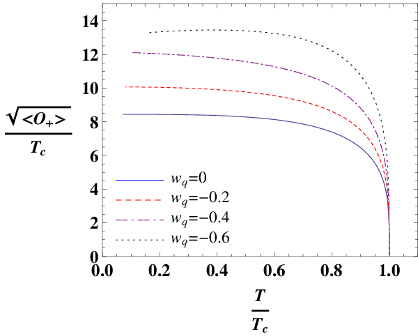

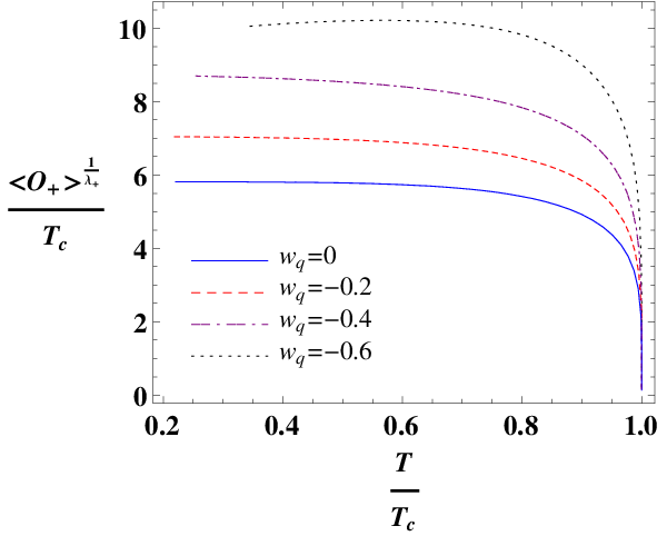
In Fig. (2), we also plot the condensates of operators and as a function of temperature with the state parameter of quintessence in the allowable region (I) for fixed in the four dimensional quintessence AdS black hole spacetime. The curves of and for the non-zero have similar behavior to those in the usual Schwarzschild AdS black hole spacetime with . Moreover, from Fig. (2), it is easy to find that the condensation gap increases with the absolute value . The similar properties of the condensation gap with the absolute value in the five dimensional black hole are shown in Fig. (3). These imply that the condensation gap becomes larger and the scalar hair is formed more difficultly in the quintessence AdS black hole spacetime.
IV The electrical conductivity
In this section we will investigate the influence of the state parameter of quintessence on the electrical conductivity. Since the condensation gap and the critical temperature depend on the state parameter , it is natural for us to examine whether the state parameter of quintessence will change the expected universal relation in the gap frequency [6]. Following the standard procedure in [5, 6], we here adopt to a sinusoidal electromagnetic perturbation . Neglecting the backreaction of the perturbational field on background metric, one can find the electromagnetic perturbation obeys the first-order perturbational equation
| (36) |


In order to avoid the complicated behavior in the gauge field falloff in dimensions higher than five, we restrict our study to the cases and . The ingoing wave boundary condition near horizon is given by
| (37) |
and the general behavior of at the asymptotic AdS region can be expressed as
| (38) |
for the case and
| (39) |
for the case , respectively. From the AdS/CFT dictionary, one can find [5] that and in the bulk corresponds to the source and the expectation value for the current on the CFT boundary, respectively. Thus, we can obtain the conductivity of the dual superconductor by using the Ohm’s law[5]
| (40) |
for the case and
| (41) |
for the case , respectively. For different values of , one can obtain the conductivity by solving the Maxwell equation numerically. We will focus on the case for the fixed scalar mass in our discussion. In Fig. (4) we plot the frequency dependent conductivity for operator obtained by solving the Maxwell equation (36) numerically for , , and at temperatures in the four dimensional quintessence AdS black hole spacetime. The solid and red dashed curves represent the real part and imaginary part of the conductivity respectively. We find a gap in the conductivity with the gap frequency . With increase of the absolute value , the gap frequency becomes larger, which means that we have larger deviations from the value for increasing absolute value of quintessence. From Fig. (5), we obtain the similar dependence of the conductivity on the state parameter in the five dimensional case. Thus, the expected universal relation in the gap frequency is really changed in the quintessence black hole AdS spacetime, which is similar to the effect of the Gauss-Bonnet coupling. Our result also show that the occurrence of holographic superconductor needs the stronger coupling in the quintessence AdS black hole spacetime.
V Summary
In this paper we obtain an exact solution of Einstein equations describing a -dimensional planar quintessence AdS black hole which depends on the state parameter of quintessence. It can reduce to the usual Schwarzschild AdS black hole as the parameter tends to zero. Applying the Sturm-Liouville analytical and numerical methods, we investigate holographic superconductors in the quintessence AdS black hole and probe effects of the state parameter on the critical temperature and the condensation formation and conductivity. The larger absolute value of leads to the lower critical temperature and make the scalar operator harder to form. Moreover, we found that the ratio between the gap frequency in the conductivity and the critical temperature becomes larger as the state parameter increases. This means that the occurrence of holographic superconductor needs the stronger coupling in the quintessence AdS black hole spacetime, which could be explained by a fact that quintessence possesses negative pressure. Our result show that the holographic superconductor share some similar features in the quintessence and Gauss-Bonnet AdS black holes. Furthermore, we also find that for the scalar condensate there exists an additional constraint condition originating from the quintessence for the operators . Beyond the allowable regions, the negative pressure of quintessence is so strong that the scalar condensate cannot be formed. For the smaller , the allowable region becomes more narrow. Moreover, the region of existing scalar condensate for the operator is smaller than that for the operator .
Finally, it is worth pointing that the dual field theoretical interpretation of the quintessence in the metric (1) is a formidable puzzle. The main reason is that the nature of quintessence in the metric (1) is still unclear at present and its form of the Lagrangian isn’t available. We leave this open issue in future. With the further investigations of the exotic components, one could interpret entirely such a black hole with quintessence in the dual theory.
Appendix A The equation of motion including backreaction
In this appendix, we will present the equation of motion including backreaction. Considering the backreaction from matter field, the metric ansatz for the -dimensional planar black hole can be expressed as
| (42) |
Substituting the metric (42) into the action
| (43) |
and then making use of the variational principle, one can obtain the equation of motion with backreaction
| (44) | |||
| (45) | |||
| (46) | |||
| (47) |
Here the Lagrangian for the quintessence could be a function of , and . Since there is no any directed coupling among the quintessence, the complex scalar field and electrical field , the energy momentum tensor originating from quintessence does not appear in the equations of motion for the fields and .
On the other hand, as in Ref.[51], the nonzero components of the energy-momentum tensor of quintessence could be constructed as a form (3) for the static spacetime (42) because that quintessence meets the equation of state in the arbitrary spacetime. Here the pressure of quintessence is defined by the average over the spatial part of the energy-momentum tensor [51], i.e., , (). According to the conservation of energy , one can find that in the spacetime (42) the energy density of quintessence obeys
| (48) |
It can be solved analytically as
| (49) |
which is consistent with Eq.(7) as we set the integration constant . Therefore, one can find that Einstein’s field equation with backreaction can be written as
| (50) | |||
| (51) |
Thus, the equation of motion for can be expressed as
| (52) |
Comparing with Eq.(44), one can find that , which means that the Lagrangian of quintessence is not an explicit function of . It is not surprising because that the Lagrangian of the electric field also possesses the similar behavior. In this spacetime (42), the Lagrangian of the electric field with the form (14) can be written as , which is not an explicit function of , but depends on . Moreover, we find that the factor in Eq.(45) can be replaced by the energy density of quintessence and then Eq.(45) can be simplified further as Eq.(50). Although quintessence does not appear explicitly in the equations of motion for the fields and Eq.(47), quintessence affects indirectly the behaviors of the scalar field , the gauge field and the quantity by the function .
Acknowledgements.
This work was partially supported by the National Natural Science Foundation of China under Grant No.11275065, the NCET under Grant No.10-0165, the PCSIRT under Grant No. IRT0964, the Hunan Provincial Natural Science Foundation of China (11JJ7001) and the construct program of key disciplines in Hunan Province. J. Jing’s work was partially supported by the National Natural Science Foundation of China under Grant Nos. 11175065, 10935013; 973 Program Grant No. 2010CB833004.References
- [1] J. M. Maldacena, Adv. Theor. Math. Phys. 2, 231 (1998).
- [2] E. Witten, Adv. Theor. Math. Phys. 2, 253 (1998).
- [3] S. S. Gubser, I. R. Klebanov, and A. M. Polyakov, Phys. Lett. B 428, 105 (1998).
- [4] O. Aharony, S. S. Gubser, J. M. Maldacena, H. Ooguri, and Y. Oz, Phys. Rept. 323, 183 (2000).
- [5] S. A. Hartnoll, C. P. Herzog and G. T. Horowitz, Phys. Rev. Lett. 101, 031601 (2008).
- [6] S. S. Gubser, Phys. Rev. D 78, 065034 (2008).
- [7] S.A. Hartnoll, Class. Quant. Grav. 26, 224002 (2009).
- [8] C.P. Herzog, J. Phys. A 42, 343001 (2009).
- [9] P. Basu, A. Mukherjee and H. H. Shieh, Phys. Rev. D 79, 045010 (2009).
- [10] C. P. Herzog, P. K. Kovtun, and D. T. Son, Phys. Rev. D 79, 066002 (2009).
- [11] S. S. Gubser, Class. Quant. Grav. 22, 5121 (2005).
- [12] R. Gregory, S. Kanno and J. Soda, J. High Energy Phys. 0910, 010 (2009).
- [13] H. Zeng, Z. Fan, Z. Ren, Phys. Rev. D 80, 066001 (2009).
- [14] S. A. Hartnoll, C. P. Herzog and G. T. Horowitz, J. High Energy Phys. 0812,015 (2008).
- [15] S. S. Gubser, Phys. Rev. Lett.101,191601 (2008).
- [16] M. M. Roberts and S. A. Hartnoll, J. High Energy Phys. 08, 035 (2008).
- [17] S. S. Gubser and S. S. Pufu, J. High Energy Phys. 11, 033 (2008).
- [18] Q. Y. Pan, B. Wang, E. Papantonopoulos, J. Oliveira and A. Pavan, Phys. Rev. D 81, 106007 (2010).
- [19] R. Cai and H. Zhang, Phys. Rev. D 81, 066003 (2010), arXiv:0911.4867.
- [20] E. J. Brynjolfsson, U.H. Danielsson, L. Thorlacius and T. Zingg, J. Phys. A 43, 065401 (2010), arXiv:0908.2611.
- [21] F. Denef and S. A. Hartnoll, Phys. Rev. D 79, 126008 (2009), arXiv:0901.1160.
- [22] S. S. Gubser, C. P. Herzog, S.S. Pufu and T. Tesileanu, Phys. Rev. Lett. 103, 141601 (2009)
- [23] J. P. Gauntlett, J. Sonner and T. Wiseman, Phys. Rev. Lett. 103,151601 (2009),arXiv:0907.3796 ; J. P. Gauntlett, J. Sonner and T. Wiseman, J. High Energy Phys.1002, 060 (2010), arXiv:0912.0512.
- [24] S. S. Gubser, S. S. Pufu and F. D. Rocha, Phys. Lett. B 683,201 (2010).
- [25] M. Ammon, J. Erdmenger, M. Kaminski and P. Kerner, Phys. Lett. B680 516 (2009); M. Ammon, J. Erdmenger, M. Kaminski and P. Kerner, J. High Energy Phys. 0910, 067 (2009).
- [26] G. T. Horowitz and M. M. Roberts, Phys. Rev. D 78, 126008 (2008).
- [27] S. S. Gubser and A. Nellore, Phys. Rev. D 80, 105007 (2009), arXiv:0908.1972.
- [28] G. T. Horowitz and M. M. Roberts, J. High Energy Phys. 0911, 015 (2009), arXiv:0908.3677.
- [29] R. A. Konoplya and A. Zhidenko, Phys. Lett. B 686, 199 (2010).
- [30] T. Nishioka, S. Ryu and T. Takayanagi, J. High Energy Phys. 1003,131 (2010).
- [31] S. Cremonesi, D. Melnikov and Y. Oz, J. High Energy Phys. 1004, 048 (2010).
- [32] F. Aprile and J. Russo, Phys. Rev. D 81, 026009 (2010).
- [33] P. Basu, J. He, A. Mukherjee and H. Shieh, Phys. Lett. B 689,45 (2010).
- [34] J. Sonner, Phys. Rev. D 80, 084031 (2009).
- [35] E. Nakano1 and W. Wen, Phys. Rev. D 78, 046004 (2008).
- [36] S. Chen, L. Wang, C. Ding and J. Jing, Nucl. Phys. B 836, 222 (2010)
- [37] K. Maeda, M. Natsuume and T. Okamura, Phys. Rev. D79,126004 (2009); K. Maeda, M. Natsuume and T. Okamura, Phys. Rev. D81, 026002 (2010).
- [38] G. Siopsis and J. Therrien, J. High Energy Phys. 1005, 013 (2010).
- [39] X.H. Ge, B. Wang, S. F. Wu, and G.H. Yang, J. High Energy Phys. 08, 108 (2010).
- [40] Y. Q. Liu, Q.Y. Pan, B. Wang, and R.G. Cai, Phys. Lett. B 693, 343 (2010).
- [41] R. G. Cai and D.W. Pang, Phys. Rev. D 84, 066004 (2011)
- [42] J. Jing, S. Chen, Phys. Lett. B 686 68 (2010).
- [43] J. Jing, Q. Pan, S. Chen, J. High Energy Phys. 1111, 45 (2011).
- [44] Q. Pan, J. Jing, B. Wang, Phys. Rev. D 84, 126020 (2011).
- [45] J. Wu, Y. Cao, X. Kuang, W. Li, Phys. Lett. B 697, 153 (2011); D. Ma, Y. Cao, J. Wu, Phys. Lett. B 704, 604 (2011).
- [46] S. Weinberg, Rev. Mod. Phys. 61, 1 (1989); V. Sahni and A. Starobinsky, Int. J. Mod. Phy. D. 9, 373 (2000); P. J. E. Peebles and B. Ratra, Rev. Mod. Phys. 75, 559 (2003); T. Padmanabhan, Phys. Rept. 380, 235 (2003).
- [47] B. Ratra and P. J. E. Peebles, Phys. Rev. D 37, 3406 (1988); P. J. E. Peebles and B. Ratra, Astrophys. J. 325, L17 (1988); C. Wetterich, Nucl. Phys. B 302, 668 (1988); R. R. Caldwell, R. Dave and P. J. Steinhardt, Phys. Rev. Lett. 80, 1582 (1998); I. Zlatev, L. Wang and P. J. Steinhardt, Phys. Rev. Lett. 82, 896 (1999); M. Doran and J. Jaeckel, Phys. Rev. D. 66, 043519 (2002).
- [48] C. A. Picon, T. Damour and V. Mukhanov, Phys. Lett. B 458, 209 (1999); T. Chiba, T. Okabe and M. Yamaguchi, Phys. Rev. D 62, 023511 (2000).
- [49] R. R. Caldwell, Phys. Lett. B 545, 23 (2002); B. McInnes, J. High Energy Phys. 08, 029 (2002); S. Nojiri and S. D. Odintsov, Phys. Lett. B 562, 147 (2003); L. P. Chimento and R. Lazkoz, Phys. Rev. Lett. 91, 211301 (2003); B. Boisseau, G. Esposito-Farese, D. Polarski, Alexei A. Starobinsky,Phys. Rev. Lett. 85, 2236 (2000); R. Gannouji, D. Polarski, A. Ranquet, A. A. Starobinsky, JCAP 0609 016(2006).
- [50] K.A. Bronnikov, J.C. Fabris, Phys. Rev. Lett. 96, 251101 (2006), arXiv:gr-qc/0511109; M. E. Rodrigues, Z. A. A. Oporto, Phys. Rev. D85, 104022 (2012), arXiv:1201.5337; D. F. Jardim, M. E. Rodrigues, M. J. S. Houndjo, arXiv:1202.2830; A. Nakonieczna, M. Rogatko, R. Moderski, Phys. Rev. D86, 044043 (2012), arXiv:1209.1203; C. J. Gao, S.N.Zhang, arXiv:hep-th/0604114.
- [51] V. V. Kiselev, Class. Quan. Grav. 20, 1187 (2003).
- [52] S. Chen, B. Wang, R. Su, Phys. Rev. D 77, 124011 (2008).
- [53] S. Chen, J. Jing, Class. Quant. Grav. 22, 4651 (2005).
- [54] Y. Zhang, Y. X. Gui, Class. Quant. Grav. 23, 6141 (2006).
- [55] I. R. Klebanov and E. Witten, Nucl. Phys. B 556, 89 (1999).