QCD phase diagram with
2-flavor lattice fermion formulations

We study the Karsten-Wilczek fermion and its symmetries in comparison with other lattice fermions with chemical potential. The $4$-d KW action with $U(1)$ chiral symmetry and ultra-locality is obtained by introducing a Wilson-like term proportional to $i\gamma_{4}$ into the naive fermion action as

where the second line with a parameter $r$ is a flavored-chemical-potential term, which works to lift the degeneracy of species. The third line with a relevant parameter $\mu_{3}$ is a dimension-3 counterterm, which corresponds to an $O(1/a)$ chemical potential term ¹¹ 1 In S. Kamata, H. Tanaka, [arXiv:1111.4536] (2011) the authors discussed difficulty of defining hermiticity in the minimal-doubling fermions. However it is always the case with lattice fermions with (imaginary) chemical potential, which lose the PT invariance. Their argument does not mean any problem peculiar to the formulations.. If one drops $i$ in front of the second and third lines, this becomes a real-type Karsten-Wilczek fermion without $\gamma_{5}$ hermiticity while we in this paper focus on the imaginary-type KW fermion basically. For the free theory, the associated Dirac operator in momentum space is given by

For $r=1$ and $\mu_{3}=0$, it has only two zeros at $p=(0,0,0,0),(0,0,0,\pi/a)$. The rest 14 species have $O(1/a)$ imaginary chemical potential due to the flavored-chemical-potential term. More precisely, among the original 16 species, two have zero imaginary chemical potential, six have $2/a$, six have $4/a$ and two have $6/a$. In the naive continuum limit, the 14 species are decoupled with infinite imaginary chemical potential and there remains only two flavors as shown in Fig. 1

. The flavored chemical potential term breaks discrete symmetries. The residual symmetries are cubic symmetry, corresponding to permutation of spatial three axes, CT and P [27]. We list the symmetries of importance as following;

(1) $U(1)$ chiral symmetry ($\gamma_{5}\otimes\tau_{3}$ [31, 30, 32, 33, 34])

(2) P

(3) CT

(4) Cubic symmetry.

Since the cubic symmetry is likely to be enhanced to the 3d rotation symmetry in the continuum, we expect that these symmetries become those of the finite-density QCD in the continuum limit. To convince ourselves, let us look into symmetries of the naive lattice fermion with chemical potential, which is introduced as a 4th-direction abelian gauge field. The massless naive action with chemical potential is given by

The chemical potential breaks the hypercubic symmetry into the spatial cubic symmetry. It also breaks C, P and T symmetries into CT and P. These discrete symmetries are the same as those of Karsten-Wilczek fermion as shown above. From the viewpoint of the universality class, these two theories belong to the same class. We therefore consider that the KW fermion suits in-medium lattice QCD much better than zero-($T$,$\mu$) lattice QCD.

However, we have to care about the way of introducing chemical potential. In KW fermions the flavored imaginary chemical potential is introduced naively as $\bar{\psi}i\gamma_{4}\psi$ while the chemical potential is usually introduced as a 4th-direction abelian gauge field on the lattice as shown in (3). As is well-known [35], the naive introduction of chemical potential violates the abelian gauge invariance and requires a counterterm to make the energy density and other thermodynamical quantities finite. We can discuss the necessity of a counterterm also from the viewpoint of the additive renormalization: We remind ourselves that the Wilson fermion breaks chiral symmetry by $O(1/a)$ flavored-mass terms, which leads to the additive mass renormalization and the necessity of the mass parameter tuning in the interacting theory. Now the KW fermion breaks discrete symmetries into those of finite-density systems by $O(1/a)$ flavored-chemical-potential terms. These facts indicate that we will here encounter large chemical potential renormalization instead of the additive mass renormalization in Wilson fermion. This is why we need to introduce the dimension-3 counterterm as $\mu_{3}\bar{\psi}i\gamma_{4}\psi$ in the action (1) even for the application to finite-density QCD. The zero-chemical-potential two flavors for a free case in (2) suffer $O(1/a)$ imaginary chemical potential renormalization in the interacting theory. We thus need to tune $\mu_{3}$ to control it even if we apply it to the finite-density QCD.

As the additive mass renormalization in Wilson fermion is manifested in the phase diagram in a ($m$–$g^{2}$) plane [36, 37, 38, 39, 40], the chemical potential renormalization can be manifested in a phase diagram in a ($\mu_{3}$–$g^{2}$) plane. The chiral phase structure in the parameter space of lattice QCD with the KW fermion is studied in [26] by using strong-coupling lattice QCD and the Gross-Neveu model: Fig. 2 is the conjectured chiral phase diagram with the number of physical flavors in the $(\mu_{3}$–$g^{2})$ plane for $r=1$. There are roughly two phases with and without chiral condensate, or equivalently with and without SSB of chiral symmetry. We name them as “physical” and “unphysical” phases since the physical QCD has SSB of chiral symmetry at least. As shown in [26], in the strong-coupling and large $N$ limits, the boundaries between the two phases are given by

which gives the physical range $-\sqrt{32/7}-3<\mu_{3}<+\sqrt{32/7}-3$ for $r=1$. We thus have the two chiral boundaries in this limit as shown in Fig. 2.

In the weak-coupling limit ($g^{2}=0$) we analytically know the number of flavors. In (2) with $r=1$, the number of flavors changes with $\mu_{3}$ being varied [26]: There are four sectors with two, six, six and two flavors as shown in Fig. 2. (On boundaries between the sectors $\mu_{3}=1,-1,-3,-5,-7$, fermions have unusual dispersions as $D(p)\sim{\bf p}+p_{4}^{2}$, which cannot be fixed even by tuning parameters. We therefore avoid these points.) There are no fermion flavors outside these four sectors, but only unphysical fermions with $O(1/a)$ chemical potential.

As seen from Fig. 2, the boundaries between physical $\langle\sigma\rangle\not=0$ and unphysical $\langle\sigma\rangle=0$ phases start from boundaries between the two-flavor and no-flavor sectors in the weak-coupling limit. It is reasonable since SSB of chiral symmetry can take place only in theories with fermions. We especially call the two-flavor range “minimal-doubling range”. For $r=1$ the minimal-doubling range is given by $-1<\mu_{3}<1$ and $-7<\mu_{3}<-5$. Toward the strong coupling limit, these ranges are expected to change with $g^{2}$ as Fig. 2. We note that the minimal-doubling range and the 6-flavor range become less distinguishable with the gauge coupling being larger.

From the viewpoints of practical application, the relevant parameter $\mu_{3}$ has to be tuned to cancel the $O(1/a)$ imaginary chemical potential renormalization for the two flavors as discussed in the previous subsection. In the weak-coupling limit, it is obvious that the two flavors feel no chemical potential as long as we set $\mu_{3}$ in the minimal-doubling range as $-1<\mu_{3}<1$ or $-7<\mu_{3}<-5$ for $r=1$. We consider that it carries over in the interacting theory: For a given gauge coupling, in order to cancel the $O(1/a)$ effective chemical potential for the two flavors, we have to set a value of $\mu_{3}$ in the minimal-doubling range. As conjectured in Fig. 2, the minimal-doubling range for the middle gauge coupling is likely to have some width, which means that we do not need to fine-tune $\mu_{3}$, just set it in the range. After we tune $\mu_{3}$ as such, there will remain only $O(1)$ renormalization of imaginary chemical potential which has a physical scale.

From these arguments, it becomes clear that KW fermion can be applied to study on the finite-($T$,$\mu$) QCD as long as $\mu_{3}$ is chosen to be a proper value. We here write the KW action with a usual chemical potential parameter $\mu$ as

where $\mu$ is a chemical potential parameter, which can be real $\mu_{\rm Re}$, imaginary $i\mu_{\rm Im}$ or complex $\mu_{\rm Re}+i\mu_{\rm Im}$. As we discussed, we consider that we can keep the additive $O(1/a)$ renormalization of imaginary chemical potential under control by setting $\mu_{3}$ within the range. We also need to adjust $\mu_{\rm Im}$ to control the $O(1)$ imaginary chemical potential. We expect we can be informed of the size of the effective imaginary chemical potential by $\pi_{4}$ condensate in small $T$ and $\mu_{\rm Re}$ region as we will discuss later.

In the end of this section, we give a comment on practical applications of KW fermions to numerical simulations. Since the present lattice simulation can be applied only to systems with small $\mu_{\rm Re}$ or with $\mu_{\rm Im}$, the most feasible application of the KW fermion for now could be the imaginary-chemical-potential lattice QCD. In such a case we can in principle describe two flavors with arbitrary $\mu_{\rm Im}$ by keeping $\mu_{3}$ within the minimal-doubling range and adjusting $\mu_{\rm Im}$ properly.

We now derive the effective potential of the scalar meson field $\sigma$ from (5) in the strong-coupling limit ($g^{2}\to\infty$). We here consider general color number $N_{c}$ for the $SU(N_{c})$ gauge group and general space-time dimensions as $d=D+1$. We first perform the 1-link integral for the gauge field in the $D$-dimensional spatial part, and introduce auxiliary fields to eliminate the 4-point interactions as

with

where we introduce the mesonic field as

We note that two auxiliary fields $\sigma$ and $\pi_{4}$ are required to get rid of four-fermi interactions in this case. $\pi_{4}$ condensate is related to density, and we will discuss it later. We also note that we dropped the next-leading order of $O(1/\sqrt{D})$ expansions in (6), which corresponds to a large $D$ limit. We now have an intermediate form of the effective action as

We here consider real chemical potential as $\mu=\mu_{\rm Re}$. We perform Fourier transformation of the temporal direction by introducing Matsubara modes as,

We here take the Polyakov gauge. The link variable in the temporal direction is given by,

with $\phi_{a}$ defined as components of gauge fields. It enables us to calculate fermionic determinant analytically as,

where we define

with $\bar{k}_{n}^{(a)}=k_{n}+\phi_{a}/N_{\tau}-i\mu$, and $\tilde{k}_{n}^{(a)}$ is determined by the relation $A\sin\tilde{k}_{n}^{(a)}=\sin\bar{k}_{n}^{(a)}+\mu_{3}+Dr-\frac{D}{2}\sqrt{1-r^{2}}\pi_{4}$. By integrating the temporal gauge field $\phi_{a}$ we derive

For $N_{c}=3$ these $Q_{n}$ are explicitly given as

As a result, the effective potential is given by

Here we redefine the free energy $4\mathcal{F}_{\rm eff}\to\mathcal{F}_{\rm eff}$ to be consistent with the phenomenological result as discussed later. We here show only the calculation result of the determinant part for $N_{c}=3$,

with

In the case of zero temperature $T=0$, we can solve the equilibrium condition analytically. For $D=3$ ($d=4$) with $m=0$ and $r=1$ the free energy is given by

In this case there are two local minima of the free energy as a function of $\sigma$, $\mathcal{F}_{\rm eff}=-\mu_{B}-\frac{3}{2}\log\left(1+(\mu_{3}+3)^{2}\right)$ at $\sigma=0$ and $\mathcal{F}_{\rm eff}=\frac{9}{2}\sigma^{2}-\frac{3}{2}\log\left(1+(\mu_{3}+3)^{2}\right)-3\mathrm{arcsinh}(3\,\sigma/\sqrt{2(1+(\mu_{3}+3)^{2})})$ at $\sigma=\sigma_{0}$. This $\sigma_{0}$ satisfies the following gap equation,

Therefore we have

Comparing these two local minima, we can show that the global minimum changes from $\sigma=\sigma_{0}$ to $\sigma=0$ at the critical chemical potential as

This phase transition is of 1st order because the order parameter $\sigma$ changes discontinuously at this critical chemical potential. We can also evaluate the baryon density $\rho_{B}=-\partial\mathcal{F}_{\rm eff}/\partial\mu_{B}$ at $T=0$. It turns out to be empty $\rho_{B}=0$ when $\mu_{B}<\mu_{B}^{\rm critical}$. On the other hand, when $\mu_{B}>\mu_{B}^{\rm critical}$, it is saturated as $\rho_{B}=1$.

We depict the QCD phase diagram with respect to chiral symmetry from the effective potential (18). We first concentrate on the case with $r=1$ for simplicity. In this case the free energy is independent of $\pi_{4}$ although it is an artifact of the strong coupling limit. Thus we simply neglect $\pi_{4}$ and set $\mu_{3}$ in the physical parameter range $(-\sqrt{32/7}<\mu_{3}+3<+\sqrt{32/7})$ in the strong-coupling limit in Fig. 2. We here take $\mu_{3}=-0.9$. In a massless case $m=0$, the phase boundary of the 2nd order chiral phase transition is given by the condition, such that the coefficient of $\sigma^{2}$ in the free energy becomes zero. When the order of the phase transition is changed from 2nd to 1st, the coefficient of $\sigma^{4}$ as well as $\sigma^{2}$ should vanish in the free energy $\mathcal{F}_{\rm eff}(\sigma)$.

Figure 3 shows the phase boundary of the chiral transition with $r=1$, $\mu_{3}=-0.9$ and $m=0$. The order of the phase transition is changed from 2nd to 1st at the tricritical point $(\mu_{B}^{\rm tri},T^{\rm tri})=(0.402,0.119)$. We also depict $\sigma$ condensate and the baryon density $\rho_{B}=-\partial\mathcal{F}_{\rm eff}/\partial\mu_{B}$ as functions of $\mu_{B}$ with several fixed $T$ in Fig. 4. We find that there are first ($T<T^{\mathrm{tri}}$) and second ($T>T^{\mathrm{tri}}$) order phase transitions for $\sigma$, followed by the phase transition of the density $\rho_{B}$. For $m\not=0$, we can easily show that the crossover transition instead appears with the 2nd-order critical point.

These results are qualitatively consistent with those with strong-coupling lattice QCD with staggered fermions, while there are some quantitative differences. For example, the KW phase diagram is suppressed in $T$ direction compared to that in staggered. We here compare the ratio of the transition baryon chemical potential at $T=0$ to the critical temperature at $\mu_{B}=0$, $R^{0}=\mu_{c}(T=0)/T_{c}(\mu_{B}=0)$. In staggered fermion, this ratio is $R^{0}_{\mathrm{st}}\simeq 3\times 0.56/(5/3)\sim 1$ [11, 12], while $R^{0}_{\mathrm{KW}}\simeq 0.406/0.178\sim 2.3$. In the real world, this ratio is larger, $R^{0}\gtrsim M_{N}/170~\mathrm{MeV}\sim 5.5$. When the finite coupling and Polyakov loop effects are taken into account for staggered fermion, $T_{c}(\mu_{B}=0)$ decreases, $\mu_{c}(T=0)$ stays almost constant, then $R^{0}$ value increases [14, 15, 16]. Larger $R^{0}$ with KW fermion in the strong coupling limit may suggest smaller finite coupling corrections in the phase boundary. Another interesting point is the location of the tricritical point. In KW fermion, the ratio $R^{\mathrm{tri}}_{\mathrm{KW}}=0.402/0.119\simeq 3.4$, while $R^{\mathrm{tri}}_{\mathrm{st}}=1.73/0.866\simeq 2.0$ for unrooted staggered fermion [11, 12]. It would be too brave to discuss this value, but $R^{\mathrm{tri}}_{\mathrm{KW}}$ is consistent with the recent Monte-Carlo simulations [42], which implies that the critical point does not exist in the low baryon chemical potential region, $\mu_{B}/T\lesssim 3$. These observations reveal usefulness of KW fermion for research on QCD phase diagram.

The $\mu_{B}$ dependence of $\sigma$ and $\rho_{B}$ seems to show there are two sequential transitions with increasing $\mu_{B}$. At $T=0.15>T^{\mathrm{tri}}$, $\sigma$ quickly decreases and $\rho_{B}$ increases at $\mu_{B}\simeq 0.25$ $(0.41)$ for $m=0$ $(0.1)$, and at a larger $\mu_{B}$ ($\mu_{B}\simeq 0.64$), increasing rate of $\rho_{B}$ as a function of $\mu_{B}$ becomes higher again. At lower temperature, $T=0.10<T^{\mathrm{tri}}$, partial restoration of the chiral symmetry is seen before the first order phase transition. Since we have not taken care of the diquark condensate, these transitions are not related to the color superconductor. Other types of matter, such as quarkyonic matter [43], partial chiral restored matter [14, 15], or nuclear matter, may be related to the above sequential change.

We next consider $r\not=1$. We as an example take $r=0.75$ and $\mu_{3}=-0.9$, which is again within the physical range. (For $r=0.75$, the physical parameter range is given by $-3.84\lesssim\mu_{3}\lesssim-0.66$ from (4).) Fig. 5 shows the phase diagram for the chiral transition, which is similar to that of $r=1$ case. We have a little higher critical temperature, $T_{c}(\mu_{B}=0)\simeq 0.20$, and a little larger transition chemical potential, $\mu_{c}(T=0)\simeq 0.42$, compared with $r=1$ case. The tricritical point, $(\mu_{B}^{\mathrm{tri}},T^{\mathrm{tri}})\simeq(0.450,0.133)$, also has a larger $T$ and $\mu_{B}$. One difference is the existence of the region, where $d\mu_{B}/dT>0$ on the first order transition boundary. This is a lattice artifact, and can be removed when we take account of finite coupling effects. The Clausius-Clapeyron relation tells us that the balance of the pressure in the coexiting two phases, I and II, leads to the slope of the phase boundary, $d\mu_{B}/dT=-(s_{\mathrm{II}}-s_{\mathrm{I}})/(\rho_{\mathrm{II}}-\rho_{\mathrm{I}})$, where $s_{i}$ and $\rho_{i}$ represent the entropy and baryon density in the phase $i$ [12]. The positive slope of the phase boundary thus implies that the entropy density in quark matter (higher $\mu_{B}$ phase) is smaller than that in hadronic matter (lower $\mu_{B}$ phase). Since the QCD phase transition is essentially the change of the degrees of freedom, we do not expect this to take place in continuum theory. In the strong copling lattice QCD, however, the baryon density is almost one in quark matter at low $T$, as discussed at $T=0$ in the previous section. In the maximum density case ($\rho_{B}=1$), all the sites are filled by $N_{c}$ quarks and the entropy is zero. Thus the entropy density can be smaller in quark matter, while this is an artifact of finite spacing lattice. The same behavior is observed in staggered fermions [11, 12], and it is found that the region with the positive slope boundary narrows or disappears with finite coupling effects in staggered fermion [15, 14, 16].

We note that in $r\not=1$ case, we have nonzero $\pi_{4}$ condensate as shown in Fig. 6, where we show $\sigma$ and $\pi_{4}$ as functions of $\mu_{B}$ for several fixed $T$. This $\pi_{4}$ condensate also undergoes a phase transition with the chiral transition. Since $\pi_{4}$ is an auxiliary field for the operator $i\bar{\psi}\gamma_{4}\psi$, an absolute value of this vector condensate is deeply related to density. The point is that this condensate still remains for $\mu_{B}=0$. It is quite natural since the $O(1)$ renormalized imaginary chemical potential $\tilde{\mu}_{\rm Im}$ due to quantum effects can survive even if we set $\mu_{3}$ in the minimal-doubling range to eliminate the $O(1/a)$ imaginary chemical potential, as we discussed in Sec. II.2. Thus, the physical imaginary chemical potential is given by the sum of the effective one $\tilde{\mu}_{\rm Im}$ and a usual $O(1)$ parameter $\mu_{\rm Im}$ as $\mu_{\rm Im}^{phys}=\tilde{\mu}_{\rm Im}+\mu_{\rm Im}$. It suggests that one possible way to control $\mu_{\rm Im}^{phys}$ in lattice QCD is to check the size of $\pi_{4}$ condensate.

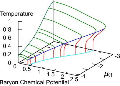
The existence of $\tilde{\mu}_{\rm Im}$ also affects the $\mu_{3}$ dependence of critical lines: In Fig. 7 we change $\mu_{3}$ and depict a three-dimensional chiral phase diagram for $T$, $\mu_{B}$ and $\mu_{3}$ for $r=1$. It shows that the critical line changes with $\mu_{3}$ being varied. As far as we keep $\mu_{3}$ in the physical range, the $O(1/a)$ effective chemical potential for the physical flavors is cancelled. As discussed above, however, we still have $O(1)$ contribution as $\tilde{\mu}_{\rm Im}$. We can interpret that the dependence of the critical line on $\mu_{3}$ comes from the dependence of $\tilde{\mu}_{\rm Im}$ on $\mu_{3}$ as $\tilde{\mu}_{\rm Im}(\mu_{3})$.

In this section we have obtained the finite-($T$,$\mu$) QCD phase diagram in the strong-coupling limit. To be precise, since the theory effectively contains the renormalized imaginary chemical potential as the KW artifact, it should be called the finite-($T$,$\mu_{\rm Re}$,$\mu_{\rm Im}$) QCD phase diagram. Anyhow, we have shown that we can apply the KW fermion to in-medium lattice QCD. We lastly discuss the real-type FCP fermions [26]. As shown in Sec. II, we can also consider the real-type KW fermion, which loses $\gamma_{5}$ hermiticity. We can perform the strong-coupling QCD analysis for this type in a parallel way, and can derive the QCD phase diagram as long as the relevant parameter is set to the physical range. In the practical lattice QCD simulations, however, we should encounter a severe sign problem with the real-type FCP fermion even for zero-density cases. We need further study to judge its applicability to lattice QCD.