Symplectic finite-difference methods for solving partial differential equations

The 1D diffusion equation

$$\frac{\partial u}{\partial t}=D\frac{\partial^{2}u}{\partial x^{2}}$$

(1)

can be solved numerically by applying the forward-time and central-difference approximations to yield the explicit algorithm

$$u_{j}^{\prime}=u_{j}+r[(u_{j+1}-u_{j})-(u_{j}-u_{j-1})],$$

(2)

where $x_{j}=j{{\Delta}x}$, $u_{j}=u(x_{j},t)$, $u_{j}^{\prime}=u(x_{j},t+{{\Delta}t})$ and

$${\it r}=\frac{{{\Delta}t}\,D}{{{\Delta}x}^{2}}.$$

(3)

Under this (Euler) algorithm, each Fourier component $\tilde{u}_{k}={\rm e}^{ikx}$ with wave number $k$ is amplified by a factor of

$$g=1-4{\it r}\sin^{2}(k{{\Delta}x}/2),$$

(4)

restricting stability ($|g|\leq 1$) to the Courant-Friedrichs-Lewy[1] (CFL) limit,

$${\it r}\leq\frac{1}{2}.$$

(5)

Since explicit finite-difference methods approximate the exact amplification factor by power-series such as (4), it seems inevitable that they will eventually blow-up and be limited in stability. However, Saul’yev[2, 3] showed in the 50’s that, by simply replacing in (2), either

$$(u_{j}-u_{j-1})\rightarrow(u_{j}^{\prime}-u_{j-1}^{\prime})\quad{\rm or}\quad(u_{j+1}-u_{j})\rightarrow(u_{j+1}^{\prime}-u_{j}^{\prime})$$

(6)

one would have unconditionally stable algorithms:

$$u_{j}^{\prime}=\beta\!_{S}\,u_{j-1}^{\prime}+\gamma\!_{S}\,u_{j}+\beta\!_{S}\,u_{j+1},$$

(7)

or

$$u_{j}^{\prime}=\beta\!_{S}\,u_{j-1}+\gamma\!_{S}\,u_{j}+\beta\!_{S}\,u^{\prime}_{j+1},$$

(8)

where $\gamma\!_{S}$ and $\beta\!_{S}$ are Saul’yev’s coefficients given by

$$\gamma\!_{S}=\frac{1-r}{1+r}\quad{\rm and}\quad\beta\!_{S}=\frac{r}{1+r}.$$

(9)

Algorithm (7) is explicit if it is evaluated in ascending order in $j$ from left to right and if the left-most $u_{1}$ is a boundary value fixed in time. Similarly, algorithm (8) is explicit if it is evaluated in descending order in $j$ from right to left and if the right-most $u_{N}$ is a boundary value fixed in time. Saul’yev also realized that both algorithms have large errors (including phase errors due to their asymmetric forms), but if they are applied alternately, the error would be greatly reduced after such a pair-wise application. This then gives rise to alternating direction explicit algorithms advocated by Larkin[4] and generalized to alternating group explicit algorithms by Evans[5, 6].

There are four unanswered questions about Saul’yev asymmetric algorithms: 1) While it is easy to show that algorithm (7) and (8) are unconditionally stable, there is no deeper understanding of this stability. 2) The algorithms are not explicit in the case of periodic boundary. What would be the algorithm if there are no fixed boundary values? 3) The alternating application of (7) and (8) greatly reduces the resulting error. How can one characterize this improvement precisely? 4) How can Saul’yev-type algorithms be generalized to higher orders?

This work presents a new way of deriving finite-difference schemes based on exponential-splittings rather than Taylor expansions. Exponential-splitting is the basis for developing symplectic integrators[7, 8, 10, 9, 11, 12, 13], the hallmark of structure-preserving algorithms. The finite-difference method presented here is properly “symplectic” in the original sense that it has certain “intertwining” quality, resembling Hamilton’s equations. It is also symplectic in the wider sense of structure-preserving, in that there is a Hamiltonian-like quantity that the algorithms seek to preserve.

As will be shown, there is a one-to-one correspondence between symplectic finite-difference methods and symplectic integrators. It is therefore useful to summarize some basic results of symplectic integrators for later reference. Symplectic integrators are based on approximating ${\rm e}^{\epsilon({\bf A}+{\bf B})}$ to any order in $\epsilon$ via a single product decomposition

$${\rm e}^{\epsilon({\bf A}+{\bf B})}=\prod_{i}{\rm e}^{a_{i}\epsilon{\bf A}}{\rm e}^{b_{i}\epsilon{\bf B}},$$

(10)

where A and B are non-commuting operators (or matrices). Usually, A+B=H is the Hamiltonian operator and ${\rm e}^{\epsilon{\bf H}}$ is the evolution operator that evolves the system forward for time $\epsilon$. The key idea is to preserve the exponential character of the evolution operator. The two first-order, Trotter[14] approximations are

$$T_{\rm 1A}(\epsilon)={\rm e}^{\epsilon{\bf A}}{\rm e}^{\epsilon{\bf B}},\quad T_{\rm 1B}(\epsilon)={\rm e}^{\epsilon{\bf B}}{\rm e}^{\epsilon{\bf A}},$$

(11)

and the two second-order Strang[15] approximations are

	$\displaystyle T_{\rm 2A}(\epsilon)$	$\displaystyle=$	$\displaystyle T_{\rm 1A}(\epsilon/2)T_{\rm 1B}(\epsilon/2)={\rm e}^{\frac{1}{2}\epsilon{\bf A}}{\rm e}^{\epsilon{\bf B}}{\rm e}^{\frac{1}{2}\epsilon{\bf A}},$
	$\displaystyle T_{\rm 2B}(\epsilon)$	$\displaystyle=$	$\displaystyle T_{\rm 1B}(\epsilon/2)T_{\rm 1A}(\epsilon/2)={\rm e}^{\frac{1}{2}\epsilon{\bf B}}{\rm e}^{\epsilon{\bf A}}{\rm e}^{\frac{1}{2}\epsilon{\bf B}}.$		(12)

The approximation

$$T_{\rm 2C}(\epsilon)=\frac{1}{2}\Bigl[T_{\rm 1A}(\epsilon)+T_{\rm 1B}(\epsilon)\Bigr]$$

(13)

is also second-order, but since it is no longer a single product of exponentials, it is no longer symplectic. In most cases, it is inferior to $T_{\rm 2A}$ and $T_{\rm 2B}$ because the time steps used in evaluating $T_{\rm 1A}$ and $T_{\rm 1B}$ are twice as large as those used in $T_{\rm 2A}$ and $T_{\rm 2B}$.

Let $T_{2}$ denotes either $T_{\rm 2A}$ or $T_{\rm 2B}$. $T_{2}$ must be second order because for a left-right symmetric product as above, it must obey

$$T_{2}(-\epsilon)T_{2}(\epsilon)=1,$$

(14)

and therefore must be of the form,

$$T_{2}(\epsilon)={\rm e}^{\epsilon{\bf H}+\epsilon^{3}{\bf E}_{3}+\epsilon^{5}{\bf E}_{5}+\cdots}$$

(15)

with only odd powers of $\epsilon$ in the exponent. (Since there is no way for the operators in (14) to cancel if there are any even power terms in $\epsilon$.) In (15), ${\bf E}_{n}$ denote higher order commutators of A and B. The algorithm corresponding to $T_{2}$ then yields exact trajectories of the second-order modified Hamiltonian

$${\bf H}_{2}(\epsilon)={\bf H}+\epsilon^{2}{\bf E}_{3}+\epsilon^{4}{\bf E}_{5}+\cdots.$$

(16)

A standard way of improving the efficiency of symplectic integrators is to generate a 2n^th-order algorithm via a product of second-order algorithms[7, 10, 9], via

$$T_{2n}(\epsilon)=\prod_{i=1}^{N}T_{2}(a_{i}\epsilon).$$

(17)

Since the error structure of $T_{2}(\epsilon)$ is given by (15), to preserve the original Hamiltonian, one must choose $a_{i}$ to perserve the first power of $\epsilon$,

$$\sum_{i=1}^{N}a_{i}=1.$$

(18)

To obtain a fourth-order algorithm, one must eliminate the error term proportinal to $\epsilon^{3}$ by requiring,

$$\sum_{i=1}^{N}a_{i}^{3}=0.$$

(19)

For a sixth-order algorithm, one must require the above and

$$\sum_{i=1}^{N}a_{i}^{5}=0,$$

(20)

and so on. While proofs of these assertions in terms of operators are not difficult, we will not need them. Symplectic finite-difference methods use a much simpler version of these ideas. Instead of dealing with the evolution operator ${\rm e}^{\epsilon{\bf H}}$, the finite difference method has a proxy, the amplification factor, which is just a function. Order-conditions such as (19) and (20) will then be obvious. Other results will be cited as needed, but these basic findings are sufficient to answer the four questions about Saul’yev’s schemes. For the next two sections we will give a detailed derivation of the symplectic diffusion and advection algorithms, followed by a discussion of the diffusion-advection equation and a concluding summary.

Consider solving the diffusion equation (1) with periodic boundary condition $u_{N+1}=u_{1}$ in the semi-discretized form,

$$\frac{du_{j}}{dt}=\frac{D}{{{\Delta}x}^{2}}(u_{j+1}-2u_{j}+u_{j-1}).$$

(21)

Regarding $u_{j}$ as a vector, this is

$$\frac{d{\bf u}}{dt}={\bf A}{\bf u},$$

(22)

with

$${\bf u}=\left(\begin{array}[]{c}u_{1}\\ u_{2}\\ \vdots\\ u_{N}\end{array}\right),\qquad{\bf A}=\frac{D}{{{\Delta}x}^{2}}\left(\begin{array}[]{ccccc}-2&1&&&1\\ 1&-2&1&&\\ &&\ddots&&\\ &&1&-2&1\\ 1&&&1&-2\\ \end{array}\right),$$

(23)

and exact solution

$${\bf u}(t+{{\Delta}t})=e^{{{\Delta}t}{\bf A}}{\bf u}(t).$$

(24)

The Euler algorithm corresponds to expanding out the exponential to first order in ${{\Delta}t}$

$${\bf u}(t+{{\Delta}t})=(1+{{\Delta}t}{\bf A}){\bf u}(t),$$

(25)

resulting in a power-series amplification factor (4), with limited stability.

If the exponential in (24) can be solved exactly, the amplification factor would be

$$g_{ex}={\rm e}^{-h_{ex}},$$

(26)

where

$$h_{ex}={\it r}4\sin^{2}(\theta/2)\quad{\rm and}\quad\theta\equiv k{{\Delta}x}.$$

(27)

The amplification exponent $h_{ex}$ here plays the role of a time parameter $r$ times the original “Hamiltonian” $h_{0}=4\sin^{2}(\theta/2)$. The resulting algorithm will then be unconditionally stable for all $r>0$. In the limit of ${{\Delta}x}\rightarrow 0$, each $k$-Fourier components will be damped by $g_{ex}={\rm e}^{-{{\Delta}t}Dk^{2}}$, which is the exact solution to (1).

To preserve this important feature of the exact solution, one must seek alternative ways of approximating of ${\rm e}^{{{\Delta}t}{\bf A}}$ without doing any Taylor expansion. The structure of ${\bf A}$ immediately suggests that it should decompose as

$${\bf A}=\sum_{j=1}^{N}{\bf A}_{j},$$

(28)

where each ${\bf A}_{j}$ has only a single, non-vanishing $2\times 2$ matrix along the diagonal connecting the $j$ and the $j+1$ elements:

$${\bf A}_{j}=\frac{D}{{{\Delta}x}^{2}}\left(\begin{array}[]{cccccc}\ddots&&&&&\\ &-1&1&&&\\ &1&-1&&&\\ &&&&&\ddots\\ \end{array}\right)\quad{\rm and}\quad{\bf A}_{N}=\frac{D}{{{\Delta}x}^{2}}\left(\begin{array}[]{cccccc}-1&&&&&1\\ &\ddots&&&&\\ &&\ddots&&&\\ 1&&&&&-1\\ \end{array}\right).$$

(29)

The exponential of each ${\bf A}_{j}$ can now be evaluated exactly:

$${\rm e}^{{{\Delta}t}{\bf A}_{j}}=\left(\begin{array}[]{cccccc}1&&&&&\\ &\alpha&\beta&&&\\ &\beta&\alpha&&&\\ &&&&&1\\ \end{array}\right),\quad\quad{\rm e}^{{{\Delta}t}{\bf A}_{N}}=\left(\begin{array}[]{cccccc}\alpha&&&&&\beta\\ &1&&&&\\ &&&1&\\ \beta&&&&&\alpha\\ \end{array}\right),$$

(30)

where

$$\alpha=\frac{1}{2}(1+\gamma),\quad\beta=\frac{1}{2}(1-\gamma),\quad{\rm and}\quad\gamma={\rm e}^{-2{\it r}}.$$

(31)

Each ${\rm e}^{{{\Delta}t}{\bf A}_{j}}$ updates only $u_{j}$ and $u_{j+1}$ as

	$\displaystyle u_{j}^{\prime}$	$\displaystyle=$	$\displaystyle\alpha u_{j}+\beta u_{j+1}$
	$\displaystyle u_{j+1}^{\prime}$	$\displaystyle=$	$\displaystyle\beta u_{j}+\alpha u_{j+1}.$		(32)

The eigenvalues of this updating matrix are $\alpha\pm\beta=1,\ \gamma$, with det $=\gamma$. This means that the updating is dissipative for $r>0$ and unstable for $r<0$. Since $\alpha$ and $\beta$ are given in terms of $\gamma$, the resulting algorithm depends only on a single parameter $\gamma$.

One can now decompose $\exp({{\Delta}t}{\bf A})$ to first order in ${{\Delta}t}$ (apply (11) repeatedly) via either

$${T}_{\rm 1A}({{\Delta}t})=e^{{{\Delta}t}{\bf A}_{N}}\cdots e^{{{\Delta}t}{\bf A}_{2}}e^{{{\Delta}t}{\bf A}_{1}},$$

(33)

or

$${T}_{\rm 1B}({{\Delta}t})=e^{{{\Delta}t}{\bf A}_{1}}\cdots e^{{{\Delta}t}{\bf A}_{N-1}}e^{{{\Delta}t}{\bf A}_{N}}.$$

(34)

These algorithms update the grid points sequentially, two by two at a time according to (32), but each grid point is updated twice, in an intertwining manner. This is crucial for dealing with the periodic boundary condition. Let $u^{*}_{j}$ denotes the first time when $u_{j}$ is updated and $u^{\prime}_{j}$ the second (and final) time it is updated. One then has for algorithm 1A:

	$\displaystyle u_{1}^{*}$	$\displaystyle=$	$\displaystyle\alpha u_{1}+\beta u_{2}$		(35)
	$\displaystyle u_{2}^{*}$	$\displaystyle=$	$\displaystyle\beta u_{1}+\alpha u_{2}$
	$\displaystyle u_{2}^{\prime}$	$\displaystyle=$	$\displaystyle\alpha u_{2}^{*}+\beta u_{3}$
	$\displaystyle u_{3}^{*}$	$\displaystyle=$	$\displaystyle\beta u_{2}^{*}+\alpha u_{3}.$
			$\displaystyle\cdots$
	$\displaystyle u_{j}^{\prime}$	$\displaystyle=$	$\displaystyle\alpha u_{j}^{*}+\beta u_{j+1}$
	$\displaystyle u_{j+1}^{*}$	$\displaystyle=$	$\displaystyle\beta u_{j}^{*}+\alpha u_{j+1}.$
			$\displaystyle\cdots$
	$\displaystyle u_{N}^{\prime}$	$\displaystyle=$	$\displaystyle\alpha u_{N}^{*}+\beta u_{1}^{*}$
	$\displaystyle u_{1}^{\prime}$	$\displaystyle=$	$\displaystyle\beta u_{N}^{*}+\alpha u_{1}^{*}.$		(36)

Since $\alpha+\beta=1$, summing up both sides from (35) to (36) gives,

$$\sum_{j=1}^{N}u^{\prime}_{j}=\sum_{j=1}^{N}u_{j}.$$

(37)

The algorithm is therefore norm-conserving. The same is true of algorithm 1B below. For $2<j<N$ one has

	$\displaystyle u_{j}^{\prime}$	$\displaystyle=$	$\displaystyle\alpha u_{j}^{*}+\beta u_{j+1}$		(38)
		$\displaystyle=$	$\displaystyle\alpha(\beta u^{*}_{j-1}+\alpha u_{j})+\beta u_{j+1}$
		$\displaystyle=$	$\displaystyle\beta(u_{j-1}^{\prime}-\beta u_{j})+\alpha^{2}u_{j}+\beta u_{j+1}$
		$\displaystyle=$	$\displaystyle\beta u_{j-1}^{\prime}+\gamma u_{j}+\beta u_{j+1}$

and for $j=2,N$,

	$\displaystyle u_{2}^{\prime}$	$\displaystyle=$	$\displaystyle\beta u_{1}^{*}+\gamma u_{2}+\beta u_{3}$
	$\displaystyle u_{N}^{\prime}$	$\displaystyle=$	$\displaystyle\beta u_{N-1}^{\prime}+\gamma u_{N}+\beta u_{1}^{*}.$		(39)

Finally when the snake bits its tail, one has

$$u_{1}^{\prime}=\frac{\beta}{\alpha}u_{N}^{\prime}+\gamma u_{1}+\frac{\gamma\beta}{\alpha}u_{2}.$$

(40)

Similarly, 1B is given by

	$\displaystyle u_{1}^{*}$	$\displaystyle=$	$\displaystyle\beta u_{N}+\alpha u_{1}$		(41)
	$\displaystyle u_{N}^{\prime}$	$\displaystyle=$	$\displaystyle\beta u_{N-1}+\gamma u_{N}+\beta u_{1}^{*}$
	$\displaystyle u_{j}^{\prime}$	$\displaystyle=$	$\displaystyle\beta u_{j-1}+\gamma u_{j}+\beta u_{j+1}^{\prime}$		(42)
	$\displaystyle u_{2}^{\prime}$	$\displaystyle=$	$\displaystyle\beta u_{1}^{*}+\gamma u_{2}+\beta u_{3}^{\prime}$
	$\displaystyle u_{1}^{\prime}$	$\displaystyle=$	$\displaystyle\frac{\gamma\beta}{\alpha}u_{N}+\gamma u_{1}+\frac{\beta}{\alpha}u_{2}^{\prime}.$		(43)

Algorithms 1A and 1B are essentially given by (38) and (42) respectively, except for three values of $u_{1}^{\prime}$, $u_{2}^{\prime}$ and $u_{N}^{\prime}$. The forms of (38) and (42) reproduce Saul’yev’s schemes (7) and (8), but with different coefficients. Saul’yev’s coefficient $\gamma\!_{S}$ is a rational approximation to the $\gamma={\rm e}^{-2r}$ here. Note that his $\beta\!_{S}=r/(1+r)$ is also given by $\beta\!_{S}=(1-\gamma\!_{S})/2$. In contrast to Saul’yev’s algorithm, which cannont be started for periodic boundary condition, algorithm 1A and 1B are truly explicit because they are fundamentally given by the sequential updating of (32). Each algorithm can get started by first updating $u_{1}$ to $u_{1}^{*}$, then updating it again at the end to $u^{\prime}_{1}$.

By virtue of (12) one can now immediately generate a second-order time-marching algorithm via the symmetric product,

	$\displaystyle{T}_{2}({{\Delta}t})$	$\displaystyle=$	$\displaystyle{T}_{\rm 1B}(\frac{{{\Delta}t}}{2}){T}_{\rm 1A}(\frac{{{\Delta}t}}{2})$		(44)
		$\displaystyle=$	$\displaystyle e^{\frac{1}{2}{{\Delta}t}{\bf A}_{1}}e^{\frac{1}{2}{{\Delta}t}{\bf A}_{2}}\cdots e^{\frac{1}{2}{{\Delta}t}{\bf A}_{N}}e^{\frac{1}{2}{{\Delta}t}{\bf A}_{N}}\cdots e^{\frac{1}{2}{{\Delta}t}{\bf A}_{2}}e^{\frac{1}{2}{{\Delta}t}{\bf A}_{1}}.$

If the boundary effects of $u_{1}^{\prime}$, $u_{2}^{\prime}$ and $u_{N}^{\prime}$ are ignored (for now) and 1A and 1B are considered as given by (38) and (42), then the alternative product ${T}_{\rm 1A}({{\Delta}t}/2){T}_{\rm 1B}({{\Delta}t}/2)$ yields the same second-order algorithm. In this case, algorithms 1A and 1B have amplification factors

	$\displaystyle g_{\rm 1A}$	$\displaystyle=$	$\displaystyle\frac{\gamma+\beta{\rm e}^{i\theta}}{1-\beta{\rm e}^{-i\theta}},$
	$\displaystyle g_{\rm 1B}$	$\displaystyle=$	$\displaystyle\frac{\gamma+\beta{\rm e}^{-i\theta}}{1-\beta{\rm e}^{+i\theta}},$		(45)

with opposite phase errors, and the second-order algorithm has

	$\displaystyle g_{2}$	$\displaystyle=$	$\displaystyle g_{\rm 1B}\left(\frac{{{\Delta}t}}{2}\right)g_{\rm 1A}\left(\frac{{{\Delta}t}}{2}\right)$		(46)
		$\displaystyle=$	$\displaystyle\frac{\widetilde{\gamma}^{2}+\widetilde{\beta}^{2}+2\widetilde{\beta}\widetilde{\gamma}\cos\!\theta}{1+\widetilde{\beta}^{2}-2\widetilde{\beta}\cos\!\theta},$
		$\displaystyle=$	$\displaystyle\frac{1-(4\widetilde{\beta}\widetilde{\gamma}/\widetilde{\alpha}^{2})\sin^{2}\!\theta/2}{1+(4\widetilde{\beta}/\widetilde{\alpha}^{2})\sin^{2}\!\theta/2}=e^{-h_{2}},$		(47)

with no phase error and where

$$\widetilde{\alpha}=\frac{1}{2}(1+\widetilde{\gamma}),\quad\widetilde{\beta}=\frac{1}{2}(1-\widetilde{\gamma})\quad{\rm and}\quad\widetilde{\gamma}=\gamma(r/2).$$

(48)

Since both algorithms 1A and 1B have phase errors, only the second-order algorithm is qualitatively similar to the exact solution. Eq.(47) makes it clear that this algorithm is unconditionally stable since $0\leq\widetilde{\gamma}\leq 1$. Algorithms 1A and 1B are also unconditionally stable since $|g_{\rm 1A,1B}|=\sqrt{g_{2}}$ with $\widetilde{\gamma}\rightarrow\gamma$. Note that this also proves the unconditional stability of Saul’yev’s algorithms. His coefficient $\gamma\!_{S}$ can turn negative, but only approaches -1 as $r\rightarrow\infty$. Conventional explicit methods, like that of the Euler algorithm, are limited in stability because they have power-series amplification factors. By contrast, symplectic finite-difference methods are unconditionally stable because they produce Saul’yev-type schemes with rational-function amplification factors. This type of stability is usually associated only with implicit methods.

Since the order of matrices defining $T_{2}({{\Delta}t})$ in (44) is left-right symmetric, one has the same situation as in the symplectic integrators case of (14), implying that $g_{2}(-r)g_{2}(r)=1$. This means that $g_{2}(-r)>1$ for all $k\neq 0$ modes and the algorithm is unconditionally unstable for negative time steps. Moreover, this also means that $h_{2}(-r)=-h_{2}(r)$ and $h_{2}(r)$ is an odd function of $r$. This is a simpler, functional version of (15). Expanding $h_{2}$ of (47) in powers of $\theta$ gives,

$$h_{2}=\frac{2(1-\widetilde{\gamma})}{1+\widetilde{\gamma}}\theta^{2}-\frac{(13-35\widetilde{\gamma}+35\widetilde{\gamma}^{2}-13\widetilde{\gamma}^{3})}{6(1+\widetilde{\gamma})^{3}}\theta^{4}+\cdots.$$

(49)

Each coefficient must be an odd function of $r$. This is satisfied only if

$$\widetilde{\gamma}(-r)\widetilde{\gamma}(r)=1.$$

(50)

Thus every function $\widetilde{\gamma}(r)$ satisfying (50) with $|\widetilde{\gamma}(r)|\leq 1$ defines an unconditionally stable algorithm for solving the diffusion equation. For the original choice of $\widetilde{\gamma}(r)={\rm e}^{-r}$, one finds

$$h_{2}=(r-\frac{r^{3}}{12}+\frac{r^{5}}{120}\cdots)\theta^{2}-(\frac{r}{12}+\frac{35r^{3}}{144}+\cdots)\theta^{4}+(\frac{r}{360}+\frac{539r^{3}}{4320}+\cdots)\theta^{6}+\cdots.$$

(51)

Comparing this to the expansion of the exact amplification exponent,

$$h_{ex}=r\theta^{2}-\frac{r}{12}\theta^{4}+\frac{r}{360}\theta^{6}+\cdots,$$

(52)

one sees that the original choice does not reproduce leading term exactly except when $r<<1$. To improve this, let’s take $\widetilde{\gamma}(r)$ to be an arbitrary function of $r$ but with $\widetilde{\alpha}$ and $\widetilde{\beta}$ still defined by (48). The first term in $h_{ex}$ can now be matched exactly by requiring

$$\frac{1-\widetilde{\gamma}(r)}{1+\widetilde{\gamma}(r)}=\frac{r}{2}\quad\rightarrow\quad\widetilde{\gamma}(r)=\frac{1-r/2}{1+r/2},$$

(53)

which is precisely Saul’yev’s original coefficient. With this choice for $\widetilde{\gamma}(r)$, (47) reads

$$g_{2}=\frac{1-2r(1-r/2)\sin^{2}(\theta/2)}{1+2r(1+r/2)\sin^{2}(\theta/2)},$$

(54)

with exponent

$$h_{2}=r\theta^{2}-(\frac{r}{12}+\frac{r^{3}}{4})\theta^{4}+(\frac{r}{360}+\frac{r^{3}}{8}+\frac{r^{5}}{16})\theta^{6}+\cdots$$

(55)

which is now correct to third-order in $\theta$. Comparing this and (51) to $h_{ex}$, one sees that all the error terms of $h_{2}$ are odd powers of $r$ higher than the first. As a matter of fact, by resumming terms proportional to $r$, we can make this error structure in exact conformity with (15),

$$h_{2}=rh_{0}+r^{3}E_{3}(\theta)+r^{5}E_{5}(\theta)+\cdots,$$

(56)

where $h_{0}=4\sin^{2}(\theta/2)$. This is the same error structure exploited by symplectic integrators to produce higher order algorithms.

Saul’yev’s algorithm is close in reproducing the amplification factor of the implicit Crank-Nicolson (CN) scheme (which is without the $\pm r/2$ terms in (54)). The CN scheme has the advantage that its exponent is

$$h_{CN}=r\theta^{2}-\frac{r}{12}\theta^{4}+(\frac{r}{360}+\frac{r^{3}}{12})\theta^{6}+\cdots$$

(57)

which is correct to fifth-order in $\theta$. In Fig.1, we compare the amplification factor of various algorithms at two values of $r$. D2 and D2S are second-order symplectic diffusion algorithms described above using the original coefficient (48) and Saul’pev’s coefficient (53), respectively. For $r=0.3$, both D2 and D2S track $g_{ex}$ closely over the entire range $k$ values. Both Euler and CN tend to over-damp higher Fourier modes. At $r=2.0$, while both Euler and CN turn negative at large $k$, D2 and D2S remain positive, like that of $g_{ex}$. At large $r$, D2S is clearly better than D2 at small $k$.

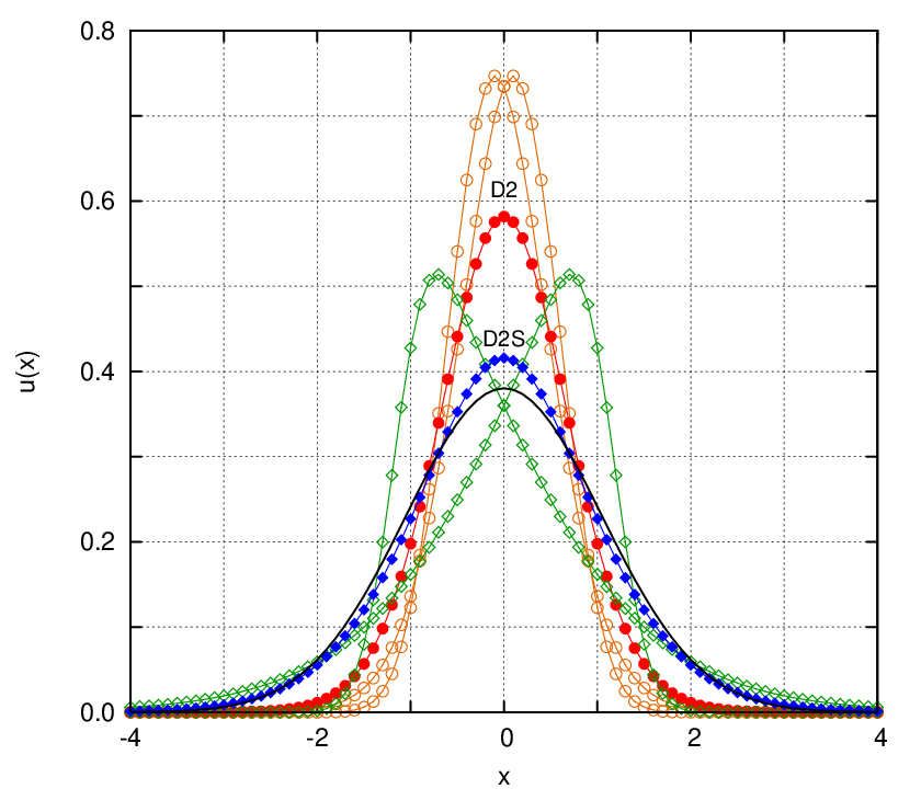
To generalize Saul’yev schemes to periodic boundary condition, one simply replaces in the above algorithms, $\gamma\rightarrow\gamma\!_{S}$. In Fig.2 we show the working of algorthms 1A, 1B and 2 using both sets of cofficients. With the original coefficients, the phase errors are much smaller, but the under-damp error is much larger. For Saul’pev’s coefficient, the phase errors are much greater, but the under-damp error is smaller. Since the phase error is automatically eliminated by going to second-order, D2S has an advantage over D2.

If one were to construct a 2n^th-order algorithm out of a product of second-order algorithms

$$T_{2n}({{\Delta}t})=\prod_{i=1}^{N}T_{2}(a_{i}{{\Delta}t}),$$

(58)

then the corresponding $h_{2n}$ is given by

	$\displaystyle h_{2n}(r)$	$\displaystyle=$	$\displaystyle\sum_{i=1}^{N}h_{2}(a_{i}r)$		(59)
		$\displaystyle=$	$\displaystyle rh_{0}\sum_{i=1}^{N}a_{i}+r^{3}E_{3}(\theta)\sum_{i=1}^{N}a^{3}_{i}+r^{5}E_{5}(\theta)\sum_{i=1}^{N}a^{5}_{i}+\cdots,$

and the order conditions (18)-(20) are easily understood. Unfortunately, for the diffusion algorithm, $T_{2}(a_{i}{{\Delta}t})$ is unstable for any negative $a_{i}$ and no negative coefficient $a_{i}$ can be allowed. In this case, order-conditions such as (19) and (20) cannot be satisfied and no higher-order composition algorithms of the form (58) is possible. (However, these algorithms will be useful for solving the advection equation in the next section.)

To overcome this impass, one must go beyond the single product approximation of (58), and consider a multi-product expansion of the form

$$T_{2n}({{\Delta}t})=\sum_{k}c_{k}\prod_{i=1}^{N_{k}}T_{2}(a_{ki}{{\Delta}t}).$$

(60)

If $a_{ki}$ were to remain positive, then Shang[16] has shown that any single product in (60) can at most be second order and that some ${c_{k}}$ coefficients must be negative. More recently this author realize that[17, 18], due to the error structure (56), the first-order term $rh_{0}$ is automatically preserved by monomial products of the form $T_{2}^{k}({{\Delta}t}/k)$ with exponent

$$h_{2}^{(k)}=rh_{0}+k^{-2}r^{3}E_{3}(\theta)+k^{-4}r^{5}E_{5}(\theta)+\cdots.$$

(61)

The arbitrariness in $N_{k}$ and $a_{ki}$ can be eliminated by taking $N_{k}=k$ and $a_{ki}=1/k$. This then produces a much simpler Multi-Product Expansion[17] (MPE)

$$T_{2n}({{\Delta}t})=\sum_{k}c_{k}T_{2}^{k}({{\Delta}t}/k)$$

(62)

for any sequence of $n$ whole numbers $\{k\}$ with analytically known coefficients $c_{k}$. For the harmonic sequence of $k=1,2,3,\cdots$, the first few higher order algorithms are:

$${T}_{4}({{\Delta}t})=-\frac{1}{3}{T}_{2}({{\Delta}t})+\frac{4}{3}{T}_{2}^{2}\left(\frac{{{\Delta}t}}{2}\right)$$

(63)

$${T}_{6}({{\Delta}t})=\frac{1}{24}{T}_{2}({{\Delta}t})-\frac{16}{15}{T}_{2}^{2}\left(\frac{{{\Delta}t}}{2}\right)+\frac{81}{40}{T}_{2}^{3}\left(\frac{{{\Delta}t}}{3}\right)$$

(64)

$${T}_{8}({{\Delta}t})=-\frac{1}{360}{T}_{2}({{\Delta}t})+\frac{16}{45}{T}_{2}^{2}\left(\frac{{{\Delta}t}}{2}\right)-\frac{729}{280}{T}_{2}^{3}\left(\frac{{{\Delta}t}}{3}\right)+\frac{1024}{315}{T}_{2}^{4}\left(\frac{{{\Delta}t}}{4}\right).$$

(65)

For the diffusion equation, the use of the fourth-order extrapolation (63) has been previously suggested by Schatzman[19]. However, these high order methods are uselss for conventional explicit schemes, since they are unstable at large time steps. It is only with the use of unconditionally stable algorithms here that the power of these high order schemes can be unleashed. These MPE algorithms do not preserve the positivity of the initial profile. This is in keeping with the general observation that there can’t be any finite-difference scheme for solving the diffusion equation that preserves positivity beyond the second-order[21]. More recently, Zillich, Mayrhofer and Chin[22] have shown that Path-Integral Monte Carlo simulations, where positivity is of the utmost importance, can be successfully carried out using these expansions, demonstrating that the violation of positivity is small and controllable. These MPE algorithms are also not symplectic. However, as argued by Blanes, Casas and Ros[20], they are symplectic to order $2n+3$. Thus at sufficiently high orders, they are indistinguishable from truly symplectic algorithms up to machine precision. In the context of classical dynamics, these MPE algorithms have been tested up to the 100^th order in Ref.18.

In Fig.3, we compare and verify the order of convergence of $T_{4}$ and $T_{6}$ with D2S as $T_{2}$ by computing the expectation value

$$\langle|x|\rangle=\frac{\sum_{j=1}^{N}|j{{\Delta}x}|u_{j}}{\sum_{j=1}^{N}u_{j}}$$

(66)

after evolving $u_{j}$ for $t=1$ as a function of ${{\Delta}t}$. The absolute value is used because the Euler algorithm would exactly preserve $\langle x\rangle$ even when it is unstable. For computing $\langle|x|\rangle$, the Euler algorithm is extremely linear within its tiny range of stability. Since it tends to over-damp, its evolving profile is flatter and $\langle|x|\rangle$ converges from above. Symplectic diffusion algorithms under-damp, and their results for $\langle|x|\rangle$ converge from below. All results can be well fitted with power laws of the form $a+b{{\Delta}t}^{n}$ with $n=1,2,4$ and 6, verifying the order of the algorithms. To show that these higher order algorithms are more efficient than running low order algorithms at reduced step sizes, we also plotted results of running the Euler algorithm 12 times at time step ${{\Delta}t}/12$ and algorithm D2S six times at ${{\Delta}t}/6$.

For the advection equation

$$\frac{\partial u}{\partial t}=-v\frac{\partial u}{\partial x},$$

(67)

its usual semi-discrete form is

$$\frac{\partial u_{j}}{\partial t}=-\frac{v}{2{{\Delta}x}}(u_{j+1}-u_{j-1}),$$

(68)

with discretization matrix

$${\bf B}=\frac{v}{2{{\Delta}x}}\left(\begin{array}[]{ccccc}0&-1&&&1\\ 1&0&-1&&\\ &&\ddots&&\\ &&1&0&-1\\ -1&&&1&0\\ \end{array}\right),$$

(69)

and solution

$${\bf u}(t+{{\Delta}t})=e^{{{\Delta}t}{\bf B}}{\bf u}(t).$$

(70)

The exact amplification factor ($\theta=k{{\Delta}x}$)

$$g_{ex}={\rm e}^{-i\eta\sin\theta},\qquad{\rm with}\qquad\eta=\frac{v{{\Delta}t}}{{{\Delta}x}},$$

(71)

is unitary and causes a phase-shift of each Fourier component. In the limit of ${{\Delta}x}\rightarrow 0$, the phase-shift becomes uniform for all the Fourier components ${\rm e}^{ikx}\rightarrow{\rm e}^{ik(x-v{{\Delta}t})}$, resulting in a uniform shift of the entire function $u(x)\rightarrow u(x-v{{\Delta}t})$, which is the exact solution to (67). Any Taylor expansion of (70) will produce algorithms with a non-unitary $g$, resulting in unwanted dissipations or instability. The situation here is much more delicate than in the diffusion case.

The natural decomposition is similarly,

$${\bf B}=\sum_{i=1}^{N}{\bf B}_{j},$$

(72)

where

$${\bf B}_{j}=\frac{v}{2{{\Delta}x}}\left(\begin{array}[]{cccccc}\ddots&&&&&\\ &0&-1&&&\\ &1&0&&&\\ &&&&&\ddots\\ \end{array}\right)\quad{\rm with}\quad{\bf B}_{N}=\frac{v}{2{{\Delta}x}}\left(\begin{array}[]{cccccc}0&&&&&1\\ &\ddots&&&&\\ &&\ddots&&&\\ -1&&&&&0\\ \end{array}\right).$$

(73)

It follows that

$${\rm e}^{{{\Delta}t}{\bf B}_{j}}=\left(\begin{array}[]{cccccc}1&&&&&\\ &c&-s&&&\\ &s&c&&&\\ &&&&&1\\ \end{array}\right),\quad\quad{\rm e}^{{{\Delta}t}{\bf B}_{N}}=\left(\begin{array}[]{cccccc}c&&&&&s\\ &1&&&&\\ &&&1&\\ -s&&&&&c\\ \end{array}\right),$$

(74)

where now

$$c=\cos(\eta/2)\quad{\rm and}\quad s=\sin(\eta/2).$$

(75)

Each ${\rm e}^{{{\Delta}t}{\bf B}_{j}}$ only updates $u_{j}$ and $u_{j+1}$ as

	$\displaystyle u_{j}^{\prime}$	$\displaystyle=$	$\displaystyle cu_{j}-su_{j+1}$
	$\displaystyle u_{j+1}^{\prime}$	$\displaystyle=$	$\displaystyle su_{j}+cu_{j+1}.$		(76)

As in the diffusion case, the above updating can be recasted into the following forms for algorithms 1A and 1B, with 1A given by

	$\displaystyle u_{1}^{*}$	$\displaystyle=$	$\displaystyle cu_{1}-su_{2}$
	$\displaystyle u_{2}^{\prime}$	$\displaystyle=$	$\displaystyle su_{1}^{*}+u_{2}-su_{3}$
	$\displaystyle u_{j}^{\prime}$	$\displaystyle=$	$\displaystyle su_{j-1}^{\prime}+u_{j}-su_{j+1}\quad(2<j<N)$		(77)
	$\displaystyle u_{N}^{\prime}$	$\displaystyle=$	$\displaystyle su_{N-1}^{\prime}+u_{N}-su_{1}^{*}$
	$\displaystyle cu_{1}^{\prime}$	$\displaystyle=$	$\displaystyle su_{N}^{\prime}+cu_{1}-su_{2}.$

and 1B given by

	$\displaystyle u_{1}^{*}$	$\displaystyle=$	$\displaystyle su_{N}+cu_{1}$
	$\displaystyle u_{N}^{\prime}$	$\displaystyle=$	$\displaystyle su_{N-1}+u_{N}-su_{1}^{*}$
	$\displaystyle u_{j}^{\prime}$	$\displaystyle=$	$\displaystyle su_{j-1}+u_{j}-su_{j+1}^{\prime}\quad(2<j<N)$		(78)
	$\displaystyle u_{2}^{\prime}$	$\displaystyle=$	$\displaystyle su_{1}^{*}+u_{2}-su_{3}^{\prime}$
	$\displaystyle cu_{1}^{\prime}$	$\displaystyle=$	$\displaystyle su_{N}+cu_{1}-su_{2}^{\prime}.$

In contrast to the diffusion case, these algorithms are not exactly norm-preserving for periodic boundary condition. By adding up both sides of the above algorithms, one finds that what is preserved by 1A is not the usual norm $N=\sum_{j=1}^{N}u_{j}$, but a modified norm given by

$$\tilde{N}_{\rm 1A}=N+(\frac{c}{1-s}-1)u_{1}$$

(79)

Similarly, what is preserved by 1B is

$$\tilde{N}_{\rm 1B}=N+(\frac{c}{1+s}-1)u_{1}.$$

(80)

If initially $u_{1}=0$, then $\tilde{N}_{\rm 1A}=\tilde{N}_{\rm 1B}=N_{0}$, where $N_{0}$ is the initial norm. As the system evolves, each algorithm’s actual norm will evolve as

	$\displaystyle N_{\rm 1A}$	$\displaystyle=$	$\displaystyle N_{0}-(\frac{c}{1-s}-1)u_{1},$
	$\displaystyle N_{\rm 1B}$	$\displaystyle=$	$\displaystyle N_{0}-(\frac{c}{1+s}-1)u_{1}.$		(81)

The error is due to a single point $u_{1}$, where it is the only point not updated twice immediately. As the wave form travels around the periodic box, $u_{1}$ will trace out the shape of the wave and imprint that as the error of the norm in time. For a sharp pulse, the norm error will return to zero after the pulse peak has passed through $u_{1}$. Thus norm-preservation will be periodic. For the advection equation, this is a small effect, and is secondary to the phase and oscillation error mentioned below. However, this error will be important in the next section.