跳到论文正文
W Papers独立论文阅读器 arXiv:1206.1634 论文正文 计算阅读时间 · 0%
引用这篇论文根据当前论文元数据生成,正式投稿前建议核对。


License: arXiv.org perpetual non-exclusive license
arXiv:1206.1634v3 [cs.NI] 24 Mar 2015

Low-Complexity Optimal Scheduling over Time-Correlated Fading Channels with
ARQ Feedback

Wenzhuo Ouyang, Atilla Eryilmaz, and Ness B. Shroff ††thanks: Wenzhuo Ouyang is with the Department of ECE, Rice University (e-mail: wenzhuo.ouyang@rice.edu). Atilla Eryilmaz is with the Department of ECE, The Ohio State University (e-mail: eryilmaz@ece.osu.edu). Ness B. Shroff holds a joint appointment in both the Department of ECE and the Department of CSE at The Ohio State University (e-mail: shroff@ece.osu.edu).††thanks: A preliminary version of this paper appeared in WiOpt 2012 [1].††thanks: This work is partly supported by NSF grants CNS-0721434, CNS-0831919, CNS-0953515, CCF-0916664, DTRA grant HDTRA 1-08-1-0016, Army Research Office MURI Awards W911NF-08-1-0238 and W911NF-07-1-0376.
Abstract

We investigate the downlink scheduling problem under Markovian ON/OFF fading channels, where the instantaneous channel state information is not directly accessible, but is revealed via ARQ-type feedback. The scheduler can exploit the temporal correlation/channel memory inherent in the Markovian channels to improve network performance. However, designing low-complexity and throughput-optimal algorithms under temporal correlation is a challenging problem. In this paper, we find that under an average number of transmissions constraint, a low-complexity index policy is throughput-optimal. The policy uses Whittle’s index value, which was previously used to capture opportunistic scheduling under temporally correlated channels. Our results build on the interesting finding that, under the intricate queue length and channel memory evolutions, the importance of scheduling a user is captured by a simple multiplication of its queue length and Whittle’s index value. The proposed queue-based index policy has provably low complexity. Numerical results show that significant throughput gains can be realized by exploiting the channel memory using the proposed low-complexity policy.

I Introduction

In wireless networks with randomly fluctuating channels, intelligently scheduling users is critical for achieving high network efficiency. Under the assumption that the scheduler possesses accurate instantaneous Channel State Information (CSI), many sophisticated scheduling algorithms have been proposed and extensively studied (e.g., [2]-[5]).

In practice, accurate instantaneous CSI is difficult to obtain at the scheduler. Hence, in this work we consider the important scenario where the instantaneous CSI is not directly accessible to the scheduler, but is instead revealed through ARQ-type feedback only after each scheduled data transmission. Many works have focused on scheduling algorithms design with imperfect CSI, where the channel state is considered independent and identically distributed (i.i.d.) processes across time (e.g., [10]-[13]). On the other hand, although the i.i.d. channel model facilitates more tractable analysis, it does not capture the time-correlation of the fading channels. ARQ-based protocols over time-correlated channels are studied in [6]-[9] under the scenarios where user scheduling is not required.

The time-correlation or channel memory inherent in the fading channels can be exploited by the scheduler for more informed decisions, and hence to obtain large throughput/utility gains (e.g., [14]-[26]). Under imperfect CSI, channel memory, and limited network resources, designing efficient scheduling schemes is highly challenging. This is because the scheduler needs to optimally balance the intricate ‘exploitation-exploration tradeoff’, i.e., to decide whether to exploit the channels with more up-to-date CSI, or to explore the channels with outdated CSI.

In this work, we study downlink scheduling with imperfect CSI and time correlated channels where, differing from works [14]-[18] in this domain, the packets destined to each user randomly arrive in time, and are stored in a corresponding observable data queue before transmission. As a result, the queue lengths randomly evolve with time. Our goal is to design scheduling algorithm that is throughput optimal, i.e., no scheduling policy can ensure system stability for arrival rates that are not supportable by the proposed scheduler. Considering queue lengths along with imperfect CSI and time correlation is highly challenging because to develop throughput-optimal scheduler requires a complex characterization of the interplay between user scheduling, channel memory evolution and queue evolution. Traditional techniques, which assume known service rate (e.g.[19][20]), or assume i.i.d. channel state process and are based on minimizing instantaneous Lyapunov drift in each slot (e.g., scheduling user with maximal instantaneous product of queue length and transmission rate [2][3]), does not apply in this context.

Under this model, because of the aforementioned complications, traditional Dynamic Programming based approaches can be used for designing scheduling schemes, but are intractable due to the well-known ‘curse of dimensionality’. In [21][22], simple round-robin based scheduling policies are shown to possess the throughput-optimality property. The optimality of greedy scheduling algorithm are proven in [23][24]. However, these schemes [21]-[24] are only optimal in the regime where users have identical ON/OFF Markovian channel statistics. In [25][26], throughput-optimal frame-based policies are proposed. These policies rely on solving a Linear Programming in each frame, which is hindered by the curse of dimensionality where the computational complexity grows exponentially with the network size.

In this work, we study throughput-optimal downlink scheduling under imperfect CSI over heterogeneous Markovian fading channels. We consider time-correlation by modeling the fading channel as an ‘ON/OFF’ Markov chain. Differing from the previous works [21]-[26] that consider scheduling problems under strict interference constraints (e.g., only one user can be scheduled at each time slot), we assume that each user occupies a dedicated channel, i.e., all users can transmit simultaneously, but the long-term average number of transmissions is limited. In this setup, we show that a low complexity scheduling policy is throughput optimal. Such a constraint on long-term average number of transmissions can be used to limit the long-term energy consumption. An example to limit the energy consumption is the green cellular networks (e.g., [27]-[29]). It is estimated that the cellular base stations consume 4.54.5 GW of power globally, which corresponds to more than 4040 million metric tons of CO2 emission and over $​10\mathdollar 10 billion electricity bill annually [27][28]. With energy expenditure rising by 1515-20%20\% each year, an important objective in green cellular networks design is to reduce the long-run average number of data transmissions to decrease energy consumption [28]. Therefore, it is of great interest to understand the relationship between the achievable throughput region and the constraint on the long-term average number of transmissions. The results proposed in this work can be applied to green cellular networks for throughput-optimal scheduling under imperfect CSI and the long-term average energy constraint.

Our contributions are as follows:

∙\bullet Under the constraint on the long-term average number of transmissions, we propose a low-complexity throughput-optimal policy. The policy operates over separate time frames and, in each time frame, tries to maximize a queue-weighted average sum-throughput. We are able to conduct a frame-based Lyapunov analysis to this policy and prove its optimality by showing that it minimizes the average Lyapunov drift over each frame. Compared to the traditional approaches for i.i.d. channels based on minimizing instantaneous Lyapunov drift each slot, the frame-based approach is useful for analysis in scenarios with time-correlated channels. The per-frame computational complexity is at most O⁡((2​τ+1)​N​log⁡(2​τ+1)​N)O((2\tau+1)N\log(2\tau+1)N) with the number of users NN, where τ\tau is a control parameter independent of NN. Therefore, the policy does not suffer from the curse of dimensionality.

∙\bullet The proposed policy builds on Whittle’s index analysis of Restless Multi-armed Bandit Problem (RMBP) [31], where Whittle’s index value is used to measure the importance of scheduling a user under the time-correlated channel [16]. Whittle’s index policies are known to have optimality properties in various RMBP processes and have been shown to have low-complexity (e.g., [15][19][20]). We find that, interestingly, under the coupled queue length and channel memory evolution, the importance of scheduling a user is measured by a simple multiplication of the queue length and Whittle’s index value that is given in closed-form. This property is essential for the low-complexity nature of our policy.

Refer to caption
Fig. 1: Two state Markov Chain model.

II System Model

II-A Downlink Scheduling Problem

We consider a time-slotted wireless downlink network with one base station and NN users, where each user ii occupies a dedicated wireless channel. The channel state of user ii, denoted by Ci​[t]C_{i}[t] at slot tt, evolves according to an ON/OFF Markov chain across time slots within the state space 𝒮={0,1}\mathcal{S}=\{0,1\}, independently across channels. When the channel is in state ‘1’, one packet can be successfully transmitted, otherwise no packet can be delivered. As shown in Fig. 1, the channel state evolution is represented by the transition probabilities

p11i:=\displaystyle p^{i}_{11}:= Pr⁡(Ci​[t]=1|Ci​[t−1]=1),\displaystyle\Pr\big(C_{i}[t]{=}1\big|C_{i}[t{-}1]{=}1\big),
p01i:=\displaystyle p^{i}_{01}:= Pr⁡(Ci​[t]=1|Ci​[t−1]=0).\displaystyle\Pr\big(C_{i}[t]{=}1\big|C_{i}[t{-}1]{=}0\big).

We assume that the Markovian channels are positively correlated, i.e., p11i>p01ip^{i}_{11}>p^{i}_{01} for i=1,2,⋯,Ni{=}1,2,\cdots,N. This assumption is commonly made in this field (e.g., [16][21][25][32]), which means that auto-correlation of the channel state process is non-negative [17]. This means, roughly speaking, that the Markov channel is more likely to stay in its state than changing to another state, which captures the typical slow fading or fast transmission scenarios. For ease of presentation, we ignore the trivial case when p11i=1p^{i}_{11}=1 or p01i=0p^{i}_{01}=0, i∈{1,⋯,N}i\in\{1,\cdots,N\}.

At the beginning of each time slot, the scheduler chooses users for data transmission. The scheduling decisions are made without the exact knowledge of the channel state in the current slot. Instead, the accurate ON/OFF channel state of a scheduled user is revealed via ACK/NACK feedback from the receiver, only at the end of each slot following data transmission.

We consider the class Φ\Phi of (possibly non-stationary) scheduling policies that make scheduling decisions based on the history of observed channel states, arrival processes, and scheduling decisions. Under the aforementioned restrictions on average energy consumption, the scheduling schemes are subject to the constraint that the long-term average number of scheduled transmissions is under MM,

lim supT→∞1T​𝔼​[∑t=0T−1∑i=1Naiϕ​[t]]≤M,\displaystyle\limsup_{T\rightarrow\infty}\frac{1}{T}\mathbb{E}\Big[\sum_{t=0}^{T-1}\sum_{i=1}^{N}a_{i}^{\phi}[t]\Big]\leq M, (1)

where aiϕ​[t]∈{0,1}a_{i}^{\phi}[t]\in\{0,1\} indicates whether user ii is scheduled at slot tt under policy ϕ∈Φ\phi\in\Phi, and M≤NM\leq N.

Data packets destined for different users are stored in separate queues before transmission. The queue length for user ii is denoted by qi​[t]q_{i}[t] at slot tt. We assume that the packet arrivals for the ii-th user form an i.i.d. process Ai​[t]A_{i}[t] with mean λi\lambda_{i} and a bounded second moment. Hence, the ii-th data queue evolves as qi​[t+1]=max⁡{0,qi​[t]−ai​[t]⋅Ci​[t]}+Ai​[t]q_{i}[t{+}1]{=}\max\{0,q_{i}[t]{-}a_{i}[t]{\cdot}C_{i}[t]\}{+}A_{i}[t].

Refer to caption
Fig. 2: Belief value evolution, p11i=0.8p^{i}_{11}=0.8, p01i=0.2p^{i}_{01}=0.2, bsi=0.5b^{i}_{s}=0.5.

II-B Belief Value Evolution

The scheduler maintains a belief value πi​[t]\pi_{i}[t] for each channel ii, defined as the probability of channel ii being in state 11 at the beginning of tt-th slot conditioned on the past channel state observations. The belief values are hence updated according to the scheduling decisions and accurate channel state feedbacks,

πi​[t+1]={p11iif ai​[t]=1 and Ci​[t]=1,p01iif ai​[t]=1 and Ci​[t]=0,Qi​(πi​[t])if ai​[t]=0,\displaystyle\pi_{i}[t+1]=\begin{cases}p^{i}_{11}&\text{if $a_{i}[t]=1$ and $C_{i}[t]=1$,}\\ p^{i}_{01}&\text{if $a_{i}[t]=1$ and $C_{i}[t]=0$,}\\ Q_{i}(\pi_{i}[t])&\text{if $a_{i}[t]=0$,}\end{cases} (2)

where Qi​(x)=x​p11i+(1−x)​p01iQ_{i}(x){=}xp^{i}_{11}+(1{-}x)p^{i}_{01} is the belief evolution operator when user ii is not scheduled in the current slot. In our setup, the belief values are known to be sufficient statistics to represent the past scheduling decisions and channel state feedback [33]. In the meanwhile, the belief value πi​[t]\pi_{i}[t] is the expected throughput for user ii if it is scheduled in slot tt.

For the ii-th user, we use bc,hib^{i}_{c,h} to denote the state of its belief value when the most recent channel state was observed hh time slots ago and was in state c∈{0,1}c\in\{0,1\}. The closed form expression of bc,hib^{i}_{c,h} can be calculated from (2) and is given as

b0,hi=p01i−(p11i−p01i)h​p01i1+p01i−p11i,b1,hi=p01i+(1−p11i)​(p11i−p01i)h1+p01i−p11i.\displaystyle b^{i}_{0,h}{=}\frac{p^{i}_{01}\hskip 1.0pt{-}\hskip 1.0pt(p^{i}_{11}{-}p^{i}_{01})^{h}p^{i}_{01}}{1+p^{i}_{01}-p^{i}_{11}},b^{i}_{1,h}{=}\frac{p^{i}_{01}{+}(1{-}p^{i}_{11})(p^{i}_{11}{-}p^{i}_{01})^{h}}{1+p^{i}_{01}-p^{i}_{11}}.

As depicted in Fig. 2, if the scheduler is never informed of the ii-th user’s channel state, the belief value monotonically converges to the stationary probability bsi:=p01i/(1+p01i−p11i)b_{s}^{i}{:=}{p^{i}_{01}}/{(1+p^{i}_{01}-p^{i}_{11})} of the channel being in state 11. We assume that the belief values of all channels are initially set to their stationary values. It is then clear that, based on (2), each belief value πi​[t]\pi_{i}[t] evolves over a countable state space, denoted by ℬi={bsi,bc,hi:c∈{0,1},h∈ℤ+}\mathcal{B}_{i}{=}\{b^{i}_{s},b^{i}_{c,h}:c\hskip 1.0pt{\in}\hskip 1.0pt\{0,1\},h\hskip 1.0pt{\in}\hskip 1.0pt\mathbb{Z}^{+}\}.

II-C Network Stability Region and Achievable Rate Region

We adopt the following definition of queue stability [3]: queue ii is stable if there exists a limiting stationary distribution FiF_{i} such that limt→∞P⁡(qi​[t]≤q)=Fi​(q)\lim_{t\rightarrow\infty}P(q_{i}[t]\leq q)=F_{i}(q). The network stability region 𝚲\bm{\Lambda} is defined as the closure of the set of arrival rate vectors supported by all policies in class Φ\Phi that does not lead to system instability while abiding by the constraint (1). A policy is called throughput optimal if, for any arrival rate vector 𝝀\bm{\lambda} within arbitrary ϵ\epsilon interior of 𝚲\bm{\Lambda}, i.e., 𝝀+ϵ​𝟏∈𝚲\bm{\lambda}+\epsilon\bm{1}\in\bm{\Lambda}, all queues are stable under the policy and constraint (1) is satisfied.

In the meanwhile, we define the achievable rate region 𝚪\bm{\Gamma} as the closure of the set of service rate vectors 𝜸\mathbf{\bm{\gamma}} that can be achieved by all policies, i.e.,

𝚪=Cl{𝜸:\displaystyle\bm{\Gamma}{=}Cl\big\{\mathbf{\bm{\gamma}}: ∃ϕ∈Φ​ with ​γi=lim infT→∞1T​𝔼​[∑t=0T−1πi​[t]⋅aiϕ​[t]],\displaystyle\exists\phi\in\Phi\text{\hskip 2.0ptwith\hskip 2.0pt}\gamma_{i}{=}\liminf_{T\rightarrow\infty}\frac{1}{T}\mathbb{E}\big[\sum_{t=0}^{T-1}\pi_{i}[t]\cdot a_{i}^{\phi}[t]\big],
i=1,⋯,N,subject to constraint(1)},\displaystyle i=1,\cdots,N,\ \text{subject to constraint}\ (\ref{eq:constraint})\big\}, (3)

where C​l​{⋅}Cl\{\cdot\} denotes the closure of the set. The rate region is convex since randomization can be performed among different policies. The achievable rate region 𝚪\bm{\Gamma} contains the set of the expected service rate vectors that can be achieved with all the policies in Φ\Phi, in the system with infinitely backlogged queues.

III Optimal Policy for Weighted Sum-throughput Maximization

In this section, we postpone discussion on queue evolution and consider a simplified problem with infinitely backlogged queues, and derive the corresponding optimal policy for weighted sum-throughput maximization. The policy introduced here, which is based on scaling the Whittle’s index values, is useful to characterize the boundary point of the achievable rate region 𝚪\bm{\Gamma}, and is also an important part in the throughput-optimal policy in the next section that stabilizes all arrival rates within the system stability region 𝚲\bm{\Lambda} – the main result of the paper.

III-A Weighted Sum-throughput Maximization Problem

Consider the following weighted sum-throughput maximization problem Ψ⁡(𝐫,M)\Psi(\mathbf{r},M) for a given vector 𝐫=(ri)i=1N\mathbf{r}=(r_{i})_{i=1}^{N}, where the expected service rate for each user ii is scaled by a non-negative factor rir_{i},

maxϕ∈Φ\displaystyle\max_{\phi\in\Phi} lim infT→∞1T​𝔼​[∑t=0T−1∑i=1Nri⋅πi​[t]⋅aiϕ​[t]]\displaystyle\ \liminf_{T\rightarrow\infty}\frac{1}{T}\mathbb{E}\Big[\sum_{t=0}^{T-1}\sum_{i=1}^{N}r_{i}{\cdot}\pi_{i}[t]{\cdot}a_{i}^{\phi}[t]\Big] (4)
s.t. lim supT→∞1T​𝔼​[∑t=0T−1∑i=1Naiϕ​[t]]≤M.\displaystyle\hskip 5.0pt\limsup_{T\rightarrow\infty}\frac{1}{T}\mathbb{E}\Big[\sum_{t=0}^{T-1}\sum_{i=1}^{N}a_{i}^{\phi}[t]\Big]\leq M. (5)

The above problem Ψ⁡(𝐫,M)\Psi(\mathbf{r},M) is hence a constrained Partially Observable Markov Decision Process (CPOMDP) [34][35].

III-B Whittle’s Index for Restless Multi-armed Bandit Problem

The problem (4)-(5) appears difficult because of the complex ‘exploitation - exploration’ tradeoff. To tackle this problem, we study it in the framework of the Restless Multiarmed Bandit Problem (RMBP) [31] and make use of the associated Whittle’s indexability analysis. We next give a brief review of the Whittle’s indices for RMBP.

RMBPs refer to a collection of sequential dynamic resource allocation problems where several independently evolving projects compete for service. In each slot, a subset of these competing projects is served. The state of each project stochastically evolves over time, based on the current state of the project and on whether the project is served in the slot. Serving a project brings a reward whose value depends on its state. Hence, in RMBPs, the controller needs to consider the fundamental tradeoff between decisions that bring high instantaneous rewards, versus those decisions that bring better future rewards but sacrifices the instantaneous rewards. Solving RMBPs are known to be PSPACE-hard [30] in general.

Whittle’s index analysis [31] for RMBPs considers the following virtual system: in each slot, the controller makes one of the two decisions for each project PP: (1) Serve project PP and accrue an immediate reward as a function of its state which is the same as in the original RMBP. (2) Do not serve project PP and obtain an immediate reward ω\omega for passivity. The state evolution of the project PP is the same as in the original RMBP, depending on its current state and current action. In this virtual system, the design goal is to maximize the long-term expected reward by balancing the ‘reward for serving’ and the ‘subsidy for passivity’ in each slot.

Letting ℐ⁡(ω)\mathcal{I}(\omega) denote the set of states of project PP in which the optimal action is to stay passive, the Whittle’s indexability condition is defined as follows.

Project PP is Whittle indexable if the set ℐ⁡(ω)\mathcal{I}(\omega) monotonically increases from ∅\emptyset to the state space 𝒮\mathcal{S} of project PP, as ω\omega increases from −∞-\infty to ∞\infty. The RMBP is Whittle indexable if every project is Whittle indexable.

If Indexability holds, for each state ss of a project, the Whittle’s index W⁡(s)W(s) is defined as the infimum of ω\omega in which it is optimal to stay idle in the ω\omega-subsidized system, i.e.,

W⁡(s)=inf{ω:s∈ℐ⁡(ω)}.\displaystyle W(s)=\inf\{\omega:s\in\mathcal{I}(\omega)\}.

Under an average constraint on the number of projects scheduled per slot, it is known that, upon the satisfaction of the Indexability condition, an optimal algorithm exists based on the ‘Whittle’s indices’: activate the projects with large Whittle’s index value [31].

The RMBP theories and the associated Whittle’s indices can be used in our downlink scheduling problem. Here, each downlink user corresponds to a project in the RMBP, with the associated state being the belief value of its channel. Correspondingly, the project is considered served if the user is scheduled for data transmission at a slot. Hence the Whittle’s index policy is very attractive to provide optimal solutions to our problem, as we shall elaborate in the rest of the paper.

III-C Optimal Policy for Weighted Sum-throughput Maximization

It was shown in that our downlink scheduling problem is Whittle indexable [18], and, under uniform weight vector 𝐫=𝟏\mathbf{r}{=}\mathbf{1}, an optimal policy for problem Ψ⁡(𝟏,M)\Psi(\mathbf{1},M) exists based on Whittle’s indexability analysis of Restless Multi-armed Bandit Problem [16]. Specifically, for channel ii, a closed form Whittle’s index value Wi𝟏​(π)W_{i}^{\mathbf{1}}(\pi) is assigned to each belief state π∈ℬi\pi\in\mathcal{B}_{i}. These indices intelligently capture the exploitation-exploration value to be gained from scheduling the user at the corresponding belief state [16]. The closed form expression of the Whittle’s index value Wi𝟏​(π),π∈ℬiW_{i}^{\mathbf{1}}(\pi),\pi\in\mathcal{B}_{i}, is given as follows [16][18],

Wi𝟏​(π)={(π−Qi​(π))​(h+1)+Qi​(π)1−p11i+(π−Qi​(π))​h+Qi​(π)if p01i≤π=b0,hi<bsip01i(1−p11i)​(1+p01i−p11i)+p11iif bsi≤π≤p11i\displaystyle W_{i}^{\mathbf{1}}(\pi){=}\hskip-3.0pt\begin{cases}\frac{(\pi-Q_{i}(\pi))(h+1)+Q_{i}(\pi)}{1-p^{i}_{11}+(\pi-Q_{i}(\pi))h+Q_{i}(\pi)}&\text{if $p^{i}_{01}{\leq}\pi{=}b^{i}_{0,h}{<}b^{i}_{s}$}\\ \frac{p^{i}_{01}}{(1-p^{i}_{11})(1+p^{i}_{01}-p^{i}_{11})+p^{i}_{11}}&\text{if $b^{i}_{s}\leq\pi\leq p^{i}_{11}$}\end{cases} (6)

It was shown that Wi𝟏​(π)W_{i}^{\mathbf{1}}(\pi) monotonically increases with π\pi and satisfies Wi𝟏​(π)∈[0,1]W_{i}^{\mathbf{1}}(\pi)\in[0,1] [16][18]. In the following lemma, we give the optimal algorithm to the problem Ψ⁡(𝐫,M)\Psi({\mathbf{r}},M) with arbitrary non-negative weight vector 𝐫\mathbf{r}. The proof of the lemma follows the line of [31] and is re-proven in Appendix A.

Lemma 1.

There exists an optimal stationary policy ϕ∗​(𝐫,M)\phi^{*}(\mathbf{r},M) for problem Ψ⁡(𝐫,M)\Psi(\mathbf{r},M) (cf. (4)-(5)), parameterized by a user index i∗i^{*}, a threshold ω∗\omega^{*} and a randomization factor ρ∗\rho^{*}, such that

(i) The scheduler maintains an 𝐫\mathbf{r}-weighted index value Wi𝐫​(πi​[t])=ri⋅Wi𝟏​(πi​[t])W^{\mathbf{r}}_{i}(\pi_{i}[t])=r_{i}\cdot W_{i}^{\mathbf{1}}(\pi_{i}[t]) for user ii.

(ii) User ii is scheduled if Wi𝐫​(πi​[t])>ω∗W^{\mathbf{r}}_{i}(\pi_{i}[t])\hskip 1.0pt{>}\hskip 1.0pt\omega^{*}, or if Wi𝐫​(πi​[t])=ω∗W^{\mathbf{r}}_{i}(\pi_{i}[t])\hskip 1.0pt{=}\hskip 1.0pt\omega^{*} with i>i∗i{>}i^{*}. User ii stays idle if  Wi𝐫​(πi​[t])<ω∗W^{\mathbf{r}}_{i}(\pi_{i}[t])\hskip 1.0pt{<}\hskip 1.0pt\omega^{*}, or if Wi𝐫​(πi​[t])=ω∗W^{\mathbf{r}}_{i}(\pi_{i}[t])\hskip 1.0pt{=}\hskip 1.0pt\omega^{*} with i<i∗i{<}i^{*}. If Wi𝐫​(πi​[t])=ω∗W^{\mathbf{r}}_{i}(\pi_{i}[t])\hskip 1.0pt{=}\hskip 1.0pt\omega^{*} with i=i∗i=i^{*}, user ii is scheduled with probability ρ∗\rho^{*}.

(iii) The parameters i∗i^{*}, ω∗\omega^{*} and ρ∗\rho^{*} are such that the long-term average number of transmissions equals MM.

Remarks: Interestingly, by multiplying the Whittle’s index values Wi𝟏​(πi​[t])W_{i}^{\mathbf{1}}(\pi_{i}[t]) with rir_{i}, the optimal policy ϕ∗​(𝟏,M)\phi^{*}(\mathbf{1},M) extends to more general problem Ψ⁡(𝐫,M)\Psi({\mathbf{r}},M). This property is important for designing the throughput-optimal policy in Section IV.

III-D Approximate i∗i^{*}, ω∗\omega^{*} and ρ∗\rho^{*} using State Space Truncation

Note that the parameters i∗i^{*}, ω∗\omega^{*} and ρ∗\rho^{*} need to be carefully chosen to satisfy the complementary slackness condition, i.e., Lemma 1(iii). While directly finding these parameters may be difficult, we next introduce an algorithm to derive approximate values of i∗i^{*}, ω∗\omega^{*} and ρ∗\rho^{*} based on a fictitious model over truncated belief state space. This fictitious model facilitates more tractable design and analysis. More importantly, we shall show that, when implementing these approximate values over the original untruncated system, the performance will get arbitrary close to the optimality.

Recall that the belief value πi​[t]\pi_{i}[t] evolves over a countable state space ℬi\mathcal{B}_{i} for user ii and approaches the stationary value if the channel is not active for a long time. This motivates us to consider the following fictitious belief evolution model over the truncated state space: the belief value of a user is set to its steady state (i.e., its channel state history is entirely forgotten) if the corresponding channel has not been scheduled for a long time, say τ\tau slots. We use πiτ​[t]\pi_{i}^{\tau}[t] to denote this ‘heuristic belief value’. The evolution of πiτ​[t]\pi_{i}^{\tau}[t] is hence,

πiτ​[t+1]=\displaystyle\pi_{i}^{\tau}[t+1]=
{p11iif ai​[t]=1 and Ci​[t]=1,p01iif ai​[t]=1 and Ci​[t]=0,Qi​(πi​[t])if ai​[t]=0, ∏k=1τ−1(1−ai​[t−k])=0,bsiif ∏k=0τ−1(1−ai​[t−k])=1.\displaystyle\begin{cases}p^{i}_{11}&\text{if $a_{i}[t]=1$ and $C_{i}[t]=1$,}\\ p^{i}_{01}&\text{if $a_{i}[t]=1$ and $C_{i}[t]=0$,}\\ Q_{i}(\pi_{i}[t])&\text{if $a_{i}[t]=0$, $\prod_{k=1}^{\tau-1}{\big(1{-}a_{i}[t{-}k]\big)}=0$,}\\ b^{i}_{s}&\text{if $\prod_{k=0}^{\tau-1}{\big(1{-}a_{i}[t{-}k]\big)}=1$.}\end{cases} (7)

We let ℬiτ\mathcal{B}_{i}^{\tau} denote the truncated state space for the ii-th user, i.e., ℬiτ={bsi,bc,li:c∈{0,1},l=1,2,⋯,τ}\mathcal{B}_{i}^{\tau}{=}\{b^{i}_{s},b^{i}_{c,l}:c\hskip 1.0pt{\in}\hskip 1.0pt\{0,1\},l\hskip 1.0pt{=}\hskip 1.0pt1,2,\cdots,\tau\} and let 𝐁τ=[ℬ1τ,⋯,ℬNτ]\mathbf{B}^{\tau}=[\mathcal{B}_{1}^{\tau},\cdots,\mathcal{B}_{N}^{\tau}]. Over the fictitious truncated state space, we consider the following policy ϕj,ω,ρt​r​u​n​c\phi^{trunc}_{j,\omega,\rho}:

Policy ϕj,ω,ρt​r​u​n​c{\phi^{trunc}_{j,\omega,\rho}} over the truncated state space: User ii is scheduled if Wi𝐫​(πiτ​[t])>ωW^{\mathbf{r}}_{i}(\pi_{i}^{\tau}[t])\hskip 1.0pt{>}\hskip 1.0pt\omega, or if Wi𝐫​(πiτ​[t])=ω∗W^{\mathbf{r}}_{i}(\pi_{i}^{\tau}[t])\hskip 1.0pt{=}\hskip 1.0pt\omega^{*} with i>ji{>}j. User ii stays idle if Wi𝐫​(πiτ​[t])<ωW^{\mathbf{r}}_{i}(\pi_{i}^{\tau}[t])\hskip 1.0pt{<}\hskip 1.0pt\omega, or if Wi𝐫​(πiτ​[t])=ω∗W^{\mathbf{r}}_{i}(\pi_{i}^{\tau}[t])\hskip 1.0pt{=}\hskip 1.0pt\omega^{*} with i<ji{<}j. If   Wi𝐫​(πiτ​[t])=ωW^{\mathbf{r}}_{i}(\pi_{i}^{\tau}[t])\hskip 1.0pt{=}\hskip 1.0pt\omega with i=ji{=}j, it is scheduled with probability ρ\rho.

Under this setup, we let the parameter αiτ​(j,ω,ρ){\alpha}^{\tau}_{i}(j,\omega,\rho) denote the long-term expected fraction of time transmitting to user ii, i.e.,

αiτ​(j,ω,ρ)=lim supT→∞1T​𝔼​[∑t=0T−1aiϕj,ω,ρt​r​u​n​c​[t]],\displaystyle{\alpha}^{\tau}_{i}(j,\omega,\rho)=\limsup_{T\rightarrow\infty}\frac{1}{T}\mathbb{E}\Big[\sum_{t=0}^{T-1}a_{i}^{\phi^{trunc}_{j,\omega,\rho}}[t]\Big], (8)

where aiϕj,ω,ρt​r​u​n​c​[t]∈{0,1}a_{i}^{\phi^{trunc}_{j,\omega,\rho}}[t]\in\{0,1\} indicates whether user ii is scheduled at time tt under policy ϕj,ω,ρt​r​u​n​c\phi^{trunc}_{j,\omega,\rho}. The closed-form expression of αiτ​(j,ω,ρ){\alpha}^{\tau}_{i}(j,\omega,\rho) is given by the following lemma. The proof of the lemma is given in Appendix B.

Lemma 2.

Let the value τ0\tau_{0} be

τ0=⌈4​max⁡{1−log⁡(p11i−p01i),1log2⁡(p11i−p01i),i=1,⋯,N}⌉.\displaystyle\hskip-9.0pt\tau_{0}{=}\Big\lceil 4\max\big\{\frac{1}{{-}\log(p^{i}_{11}{-}p^{i}_{01})},\frac{1}{\log^{2}(p^{i}_{11}{-}p^{i}_{01})},i{=}1,{\cdots},N\big\}\Big\rceil. (9)

Over the truncated state space and under policy ϕj,ω,ρt​r​u​n​c\phi^{trunc}_{j,\omega,\rho}, if τ>τ0\tau>\tau_{0}, the following hold for αiτ​(j,ω,ρ){\alpha}^{\tau}_{i}(j,\omega,\rho),

(i) The closed-form expression of αjτ​(j,ω,ρ){\alpha}^{\tau}_{j}(j,\omega,\rho) is given by

αjτ​(j,ω,ρ)\displaystyle{\alpha}^{\tau}_{j}(j,\omega,\rho)
=\displaystyle={\hskip-5.0pt} {ρ⁡(b0,hj−b0,h+1j)+1−p11j+b0,h+1jρ​b0,hj+(1−ρ)​b0,h+1j+(1−p11j)​(h+1−ρ)if ω=Wj𝐫​(b0,hj), h<τρ⁡(b0,τj−bsj)+1−p11j+bsjρ​b0,τj+(1−ρ)​bsj+(1−p11j)​(τ+1−ρ)if ω=Wj𝐫​(b0,τj)ρ⁡(1−p11j+bsj)(1+τ​ρ)​(1−p11j)+ρ​bsjif ω=Wj𝐫​(bsj)0if ω>Wj𝐫​(bsj).\displaystyle\begin{cases}\frac{\rho(b^{j}_{0,h}-b^{j}_{0,h+1})+1-p^{j}_{11}+b^{j}_{0,h{+}1}}{\rho b^{j}_{0,h}{+}(1{-}\rho)b^{j}_{0,h\hskip-1.0pt{+}\hskip-1.0pt1}{+}(1\hskip-1.0pt{-}\hskip-1.0ptp^{j}_{11})(h{+}1{-}\rho)}&\text{if $\omega{=}W^{\mathbf{r}}_{j}(b^{j}_{0,h})$, $h{<}\tau$}\\ \frac{\rho(b^{j}_{0,\tau}-b^{j}_{s})+1-p^{j}_{11}+b^{j}_{s}}{\rho b^{j}_{0,\tau}+(1-\rho)b^{j}_{s}+(1-p^{j}_{11})(\tau+1-\rho)}&\text{if $\omega{=}W^{\mathbf{r}}_{j}(b^{j}_{0,\tau})$}\\ \frac{\rho(1-p^{j}_{11}+b^{j}_{s})}{(1+\tau\rho)(1-p^{j}_{11})+\rho b^{j}_{s}}&\text{if $\omega{=}W^{\mathbf{r}}_{j}(b^{j}_{s})$}\\ 0&\text{if $\omega{>}W^{\mathbf{r}}_{j}(b^{j}_{s})$.}\end{cases}

The closed-form expression of αiτ​(j,ω,ρ),i≠j{\alpha}^{\tau}_{i}(j,\omega,\rho),i\neq j is given by

αiτ​(j,ω,ρ)\displaystyle{\alpha}^{\tau}_{i}(j,\omega,\rho)
=\displaystyle={\hskip-5.0pt} {1−p11i+b0,h+1ib0,h+1i+(1−p11i)​(h+1)if h<τ, ω=Wi𝐫​(b0,hi), i<j1−p11i+b0,hib0,hi+(1−p11i)​hif h≤τ, ω=Wi𝐫​(b0,hi), i>j;or if h≤τ,Wi𝐫​(b0,h−1i)<ω<Wi𝐫​(b0,hi)1−p11i+bsibsi+(1−p11i)​(τ+1)if ω=Wi𝐫​(b0,τi), i<j;or if ω=Wi𝐫​(bsi), i>j0if ω=Wi𝐫​(bsi), i<j;or if ω>Wi𝐫​(bsi).\displaystyle\begin{cases}\frac{1-p^{i}_{11}+b^{i}_{0,h{+}1}}{b^{i}_{0,h{+}1}{+}(1{-}p^{i}_{11})(h{+}1)}&\text{if $h{<}\tau$, $\omega{=}W^{\mathbf{r}}_{i}(b^{i}_{0,h})$, $i{<}j$}\\ \frac{1-p^{i}_{11}+b^{i}_{0,h}}{b^{i}_{0,h}{+}(1{-}p^{i}_{11})h}&\text{if $h{\leq}\tau$, $\omega{=}W^{\mathbf{r}}_{i}(b^{i}_{0,h})$, $i>j$;}\\ &\text{or if $h{\leq}\tau$,$W^{\mathbf{r}}_{i}(b^{i}_{0,h{-}1}){<}\omega{<}W^{\mathbf{r}}_{i}(b^{i}_{0,h})$}\\ \frac{1-p^{i}_{11}+b^{i}_{s}}{b^{i}_{s}+(1-p^{i}_{11})(\tau+1)}&\text{if $\omega{=}W^{\mathbf{r}}_{i}(b^{i}_{0,\tau})$, $i<j$;}\\ &\text{or if $\omega{=}W^{\mathbf{r}}_{i}(b^{i}_{s})$, $i>j$}\\ 0&\text{if $\omega{=}W^{\mathbf{r}}_{i}(b^{i}_{s})$, $i<j$;}\\ &\text{or if $\omega{>}W^{\mathbf{r}}_{i}(b^{i}_{s})$.}\end{cases}

(ii) For fixed πj∈{b0,1j,b0,2j,⋯,b0,τj,bsj}\pi_{j}{\in}\{b^{j}_{0,1},b^{j}_{0,2},{\cdots},b^{j}_{0,\tau},b^{j}_{s}\}, αjτ​(j,Wj𝐫​(πj),ρ){\alpha}^{\tau}_{j}(j,W_{j}^{\mathbf{r}}(\pi_{j}),\rho) strictly increases with ρ\rho. For fixed ρ\rho, αiτ​(j,Wi𝐫​(πi),ρ){\alpha}^{\tau}_{i}(j,W_{i}^{\mathbf{r}}(\pi_{i}),\rho) strictly decreases with πi\pi_{i} for πi∈{b0,1i,b0,2i,⋯,b0,τi,bsi}\pi_{i}\in\{b^{i}_{0,1},b^{i}_{0,2},\cdots,b^{i}_{0,\tau},b^{i}_{s}\} and all ii.

We approximate the optimal values i∗i^{*}, ω∗\omega^{*} and ρ∗\rho^{*} (defined in Lemma 1) using the fictitious truncated state space model. The approximate value iτi_{\tau}, ωτ\omega_{\tau} and ρτ\rho_{\tau} are such that, under policy ϕiτ,ωτ,ρτt​r​u​n​c\phi^{trunc}_{i_{\tau},\omega_{\tau},\rho_{\tau}} over the truncated state space, the long-term average number of transmissions equals MM, i.e.,

∑i=1Nαiτ​(iτ,ωτ,ρτ)=M.\displaystyle\sum_{i=1}^{N}{\alpha}^{\tau}_{i}(i_{\tau},\omega_{\tau},\rho_{\tau})=M. (10)

Note that, equation (10) is the truncated-state-space correspondence of Lemma 1(iii). We next design an algorithm, denoted by Gτ​(𝐫,M)G^{\tau}(\mathbf{r},M), to calculate iτi_{\tau}, ωτ\omega_{\tau} and ρτ\rho_{\tau}, described to the right and explained next.

Algorithm Gτ​(𝐫,M)G^{\tau}(\mathbf{r},M): Calculation of iτi_{\tau}, ωτ\omega_{\tau} and ρτ\rho_{\tau}
1: TxTime​[i]=1​ for all i∈{1,⋯,N}\text{TxTime}[i]=1\text{ for all $i\in\{1,\cdots,N\}$}
2: TotalTime=N\text{TotalTime}=N
3: struct Index
4: {\{ float value
5:   int user
6: }\} 𝐈⁡[(2​τ+1)​N],𝐰⁡[(2​τ+1)​N]\mathbf{I}[(2\tau+1)N],\mathbf{w}[(2\tau+1)N]
7: j=0j=0
8: for i=1i=1 to NN do
9:   for each πi∈ℬiτ\pi_{i}\in\mathcal{B}_{i}^{\tau} do
10:    Wi𝐫​(πi)=ri⋅Wi𝟏​(πi)W_{i}^{\mathbf{r}}(\pi_{i})=r_{i}\cdot W_{i}^{\mathbf{1}}(\pi_{i})
11:    𝐈⁡[j].\mathbf{I}[j].value=Wi𝐫​(πi)=W_{i}^{\mathbf{r}}(\pi_{i})
12:    𝐈⁡[j].\mathbf{I}[j].user=i=i
13:    j←j+1j\leftarrow j+1
14:   end for
15: end for
16: 𝐰=\mathbf{w}=sort(𝐈)(\mathbf{I}) ⊳\triangleright Sort the elements in 𝐈\mathbf{I} in increasing order
17:        of the index value and outputs to vector 𝐰\mathbf{w}.
18:        For index values that are equal, they are or-
19:        dered in increasing order of the associated
20:        user index.
21: for k=1k=1 to size(𝐰)(\mathbf{w}) do
22:   NewTime[𝐰[k].user]=α𝐰⁡[k].userτ(𝐰[k].value,1)\text{NewTime}[\mathbf{w}[k].\text{user}]={\alpha}^{\tau}_{\mathbf{w}[k].\text{user}}(\mathbf{w}[k].\text{value},1)
23:   TimeDiff=TxTime[𝐰[k].user]−NewTime[𝐰[k].user]\text{TimeDiff}=\text{TxTime}[\mathbf{w}[k].\text{user}]{-}\text{NewTime}[\mathbf{w}[k].\text{user}]
24:   TotalTime=TotalTime−TimeDiff\text{TotalTime}=\text{TotalTime}-\text{TimeDiff}
25:   if TotalTime<M\text{TotalTime}<M then
26:    iτ=𝐰⁡[k−1].useri_{\tau}=\mathbf{w}[k-1].\text{user}
27:    ωτ=𝐰⁡[k−1].value\omega_{\tau}=\mathbf{w}[k{-}1].\text{value}
28:    TxTime[𝐰[k−1].user]=M−∑i≠𝐰⁡[k−1].userTxTime[i]\text{TxTime}[\mathbf{w}[k{-}1].\text{user}]=M{-}\hskip-9.0pt\sum\limits_{i\neq\mathbf{w}[k{-}1].\text{user}}\hskip-9.0pt\text{TxTime}[i]
29:    ρτ=β𝐰⁡[k−1].user(ωτ,TxTime[𝐰[k−1].user])\rho_{\tau}=\beta_{\mathbf{w}[k{-}1].\text{user}}(\omega_{\tau},\text{TxTime}[\mathbf{w}[k{-}1].\text{user}])
30:    Break
31:   end if
32:   TxTime[𝐰[k].user]=NewTime[𝐰[k].user]\text{TxTime}[\mathbf{w}[k].\text{user}]{=}\text{NewTime}[\mathbf{w}[k].\text{user}]
33: end for
34: return ωτ\omega_{\tau}, ρτ\rho_{\tau}

∙\bullet The algorithm first calculates the 𝐫\mathbf{r}-weighted index values Wi𝐫​(πi)W_{i}^{\mathbf{r}}(\pi_{i}) by scaling Wi𝟏​(πi)W_{i}^{\mathbf{1}}(\pi_{i}) by rir_{i}, and stores the value and the corresponding user in vector 𝐈\mathbf{I} (line 7-15).

∙\bullet The algorithm then sorts all the 𝐫\mathbf{r}-weighted indices of each belief state of all users to a (2​τ+1)​N(2\tau{+}1)N-dimensional vector 𝐰\mathbf{w} in increasing order (line 16).

∙\bullet The algorithm then calculates ωτ\omega_{\tau} and ρτ\rho_{\tau} based on the monotonicity property in Lemma 2(ii). Hence, fixing the randomization factor ρ=1\rho{=}1, it increases the threshold ω\omega by going through the indices in 𝐰\mathbf{w} and calculates the long-term average number of transmission when threshold ω\omega equals to that index. For each element of 𝐰\mathbf{w}, it first calculates the long-term expected fraction of time NewTime[𝐰[k].user]\text{NewTime}[\mathbf{w}[k].\text{user}] transmitting to the corresponding user 𝐰⁡[k].user\mathbf{w}[k].\text{user} in line 18, and hence the decreased amount, denoted by TimeDiff, as compared with previous value TxTime[𝐰[k].user]\text{TxTime}[\mathbf{w}[k].\text{user}] in line 19. Note that, in each iteration, only the user corresponding to 𝐰⁡[k]\mathbf{w}[k] will have an updated expected fraction of transmission time. The total expected number of transmission, denoted by TotalTime, is then updated by decreasing the same amount (line 20). The threshold ω\omega keeps increasing until the total expected number of transmission is below MM (line 21). Noting that αiτ​(ω,1){\alpha}^{\tau}_{i}(\omega,1) decreases with ω\omega, we then set iτ=𝐰⁡[k−1].useri_{\tau}=\mathbf{w}[k-1].\text{user} and ωτ=𝐰⁡[k−1].value\omega_{\tau}=\mathbf{w}[k-1].\text{value} (line 21-22). Then we calculate the expected transmission time to the user that corresponds to 𝐰⁡[k−1]\mathbf{w}[k-1] (line 23) and select the randomization factor ρτ\rho_{\tau} so that the constraint (10) is satisfied (line 24), where the function βi:(ω,α)→ρ\beta_{i}:(\omega,\alpha)\rightarrow\rho calculates the randomization factor ρ\rho required to achieve the long-term expected fraction of time α\alpha transmitting to user ii at threshold ω\omega, and is derived from lemma 2(i) as,

βi​(ω,α)\displaystyle\beta_{i}(\omega,\alpha)
=\displaystyle={\hskip-5.0pt} {(1−α)​(1−p11i+b0,h+1i)−α​h​(1−p11i)(1−α)​(b0,h+1i−b0,hi)−α⁡(1−p11i)if ω=Wi𝐫​(b0,hi), h<τ;(1−α)​(1−p11i+bsi)−α​τ​(1−p11i)(1−α)​(bsi−b0,τi)−α⁡(1−p11i)if ω=Wi𝐫​(b0,τi);α⁡(1−p11i)(1−α​τ)​(1−p11i)+(1−α)​bsiif ω=Wi𝐫​(bsi);0if ω>Wi𝐫​(bsi).\displaystyle\begin{cases}\frac{(1-\alpha)(1-p^{i}_{11}+b^{i}_{0,h+1})-\alpha h(1-p^{i}_{11})}{(1-\alpha)(b^{i}_{0,h+1}-b^{i}_{0,h})-\alpha(1\hskip-1.0pt{-}\hskip-1.0ptp^{i}_{11})}&\text{if $\omega{=}W^{\mathbf{r}}_{i}(b^{i}_{0,h})$, $h{<}\tau$;}\\ \frac{(1-\alpha)(1-p^{i}_{11}+b^{i}_{s})-\alpha\tau(1-p^{i}_{11})}{(1-\alpha)(b^{i}_{s}-b^{i}_{0,\tau})-\alpha(1\hskip-1.0pt{-}\hskip-1.0ptp^{i}_{11})}&\text{if $\omega{=}W^{\mathbf{r}}_{i}(b^{i}_{0,\tau})$;}\\ \frac{\alpha(1-p^{i}_{11})}{(1-\alpha\tau)(1-p^{i}_{11})+(1-\alpha)b^{i}_{s}}&\text{if $\omega{=}W^{\mathbf{r}}_{i}(b^{i}_{s})$;}\\ 0&\text{if $\omega{>}W^{\mathbf{r}}_{i}(b^{i}_{s})$.}\end{cases}

III-E Performance of policy over untruncated state space with approximate parameters ωτ,ρτ\omega_{\tau},\rho_{\tau}

We next examine, over the original untruncated model, the policy that uses the approximated parameters iτi_{\tau}, ωτ\omega_{\tau} and ρτ\rho_{\tau}. We denote such policy as ϕτ​(𝐫,M)\phi_{\tau}(\mathbf{r},M) and present it next.

Algorithm ϕτ​(𝐫,M)\phi_{\tau}(\mathbf{r},M): 𝐫\mathbf{r}-weighted Index Policy
1: Initialization phase: The parameters iτi_{\tau}, ωτ\omega_{\tau} and ρτ\rho_{\tau} are calculated by algorithm Gτ​(𝐫,M)G^{\tau}(\mathbf{r},M).
2: At slot t\bm{t}: user ii is scheduled if the 𝐫\mathbf{r}-weighted index value Wi𝐫​(πi​[t])>ωτW^{\mathbf{r}}_{i}(\pi_{i}[t])>\omega_{\tau}, or if Wi𝐫​(πi​[t])=ωτW^{\mathbf{r}}_{i}(\pi_{i}[t]){=}\omega_{\tau} with i>iτi{>}i_{\tau}. User ii stays passive if  Wi𝐫​(πi​[t])<ωτW^{\mathbf{r}}_{i}(\pi_{i}[t])<\omega_{\tau}, or if Wi𝐫​(πi​[t])=ωτW^{\mathbf{r}}_{i}(\pi_{i}[t])\hskip 1.0pt{=}\hskip 1.0pt\omega_{\tau} with i<iτi{<}i_{\tau}. If Wi𝐫​(πi​[t])=ωτW^{\mathbf{r}}_{i}(\pi_{i}[t]){=}\omega_{\tau} with i=iτi{=}i_{\tau}, user ii is scheduled with probability ρτ\rho_{\tau}.

Remark: The computational complexity of the initialization phase of algorithm ϕτ​(𝐫,M)\phi_{\tau}(\mathbf{r},M) is dominated by sorting the index values in Algorithm Gτ​(𝐫,M)G^{\tau}(\mathbf{r},M) (line 16), which has complexity O⁡((2​τ+1)​N⋅log⁡((2​τ+1)​N))O\big((2\tau+1)N\cdot\log\big((2\tau+1)N\big)\big). After initialization, the 𝐫\mathbf{r}-weighted Index Policy ϕτ​(𝐫,M)\phi_{\tau}(\mathbf{r},M) takes a very simple threshold-type form with per-slot computational complexity O⁡(N)O(N).

We let V∗​(𝐫,M)V^{*}(\mathbf{r},M) be the weighted sum-throughput under the optimal policy ϕ∗​(𝐫,M)\phi^{*}(\mathbf{r},M) defined in lemma 1, and let Vτ​(𝐫,M)V_{\tau}(\mathbf{r},M) be that under the afore-mentioned policy ϕτ​(𝐫,M)\phi_{\tau}(\mathbf{r},M), i.e.,

V∗​(𝐫,M)=lim infT→∞1T​𝔼​[∑t=0T−1∑i=1Nri⋅πi​[t]⋅aiϕ∗​(𝐫,M)​[t]].\displaystyle V^{*}(\mathbf{r},M){=}\liminf_{T\rightarrow\infty}\frac{1}{T}\mathbb{E}\Big[\sum_{t=0}^{T-1}\sum_{i=1}^{N}r_{i}{\cdot}\pi_{i}[t]{\cdot}a_{i}^{\phi^{*}(\mathbf{r},M)}[t]\Big]. (11)
Vτ​(𝐫,M)=lim infT→∞1T​𝔼​[∑t=0T−1∑i=1Nri⋅πi​[t]⋅aiϕτ​(𝐫,M)​[t]].\displaystyle V_{\tau}(\mathbf{r},M){=}\liminf_{T\rightarrow\infty}\frac{1}{T}\mathbb{E}\Big[\sum_{t=0}^{T-1}\sum_{i=1}^{N}r_{i}{\cdot}\pi_{i}[t]{\cdot}a_{i}^{\phi_{\tau}(\mathbf{r},M)}[t]\Big]. (12)

Since we also require the long-term average number of transmissions of the policy ϕτ​(𝐫,M)\phi_{\tau}(\mathbf{r},M) to satisfy the constraint (1), we denote Zτ​(𝐫,M)Z_{\tau}(\mathbf{r},M) as the time-average expected number of transmissions under this policy, i.e.,

Zτ​(𝐫,M)=lim supT→∞1T​𝔼​[∑t=0T−1∑i=1Naiϕτ​(𝐫,M)​[t]].\displaystyle Z_{\tau}(\mathbf{r},M)=\limsup_{T\rightarrow\infty}\frac{1}{T}\mathbb{E}\Big[\sum_{t=0}^{T-1}\sum_{i=1}^{N}a_{i}^{\phi_{\tau}(\mathbf{r},M)}[t]\Big].

Recall that τ0\tau_{0} is defined in Lemma 2. The next lemma shows that the policy ϕτ​(𝐫,M)\phi_{\tau}(\mathbf{r},M) asymptotically achieves the maximum weighted sum-throughput of (4)(5) as the truncation size increases, while abiding the long-term average number of transmissions constrain (1). The proof is given in Appendix C.

Lemma 3.

For τ≥τ0\tau\geq\tau_{0}, we have

(i) The weighted sum-throughput performance difference between the policies ϕ∗​(𝐫,M)\phi^{*}(\mathbf{r},M) and ϕτ​(𝐫,M)\phi_{\tau}(\mathbf{r},M) is bounded by

|V∗​(𝐫,M)−Vτ​(𝐫,M)|≤f⁡(τ)​∑i=1Nri,\displaystyle|V^{*}(\mathbf{r},M)-V_{\tau}(\mathbf{r},M)|\leq f(\tau)\sum_{i=1}^{N}r_{i}, (13)

where f⁡(τ)=∑i=1Nfi​(τ)f(\tau){=}\sum_{i=1}^{N}f_{i}(\tau), which satisfies f⁡(τ)→0f(\tau){\rightarrow}0 as τ→∞\tau{\rightarrow}\infty with

fi​(τ)=ρ⁡(b0,τi−b0,τ+1i)+1−p11i+b0,τ+1iρ​b0,τi+(1−ρ)​b0,τ+1i+(1−p11i)​(τ+1−ρ).\displaystyle f_{i}(\tau)=\frac{\rho(b^{i}_{0,\tau}-b^{i}_{0,\tau+1})+1-p^{i}_{11}+b^{i}_{0,\tau{+}1}}{\rho b^{i}_{0,\tau}{+}(1{-}\rho)b^{i}_{0,\tau\hskip-1.0pt{+}\hskip-1.0pt1}{+}(1\hskip-1.0pt{-}\hskip-1.0ptp^{i}_{11})(\tau{+}1{-}\rho)}. (14)

(ii) The long-term average number of transmissions under policy ϕτ​(𝐫,M)\phi_{\tau}(\mathbf{r},M) satisfies the constraint (1), i.e., Zτ​(𝐫,M)≤MZ_{\tau}(\mathbf{r},M)\leq M.

Remark: Note that the truncation size τ\tau needs to be sufficiently large (i.e., τ≥τ0\tau\geq\tau_{0}) to prove the Lemma. This is because sufficiently large truncation size can provide enough level of approximation that facilitates analytical characterization. Specifically, in the proof, τ0\tau_{0} is used in Lemma 4.

IV QUEUE-BASED INDEX POLICY OVER TIME FRAMES

Note that the Index Policy in the last section, as well as the associated Whittle’s index value, is for the system with infinitely backlogged queues and the corresponding weighted sum-throughput maximization problem (4)-(5). In this section, we consider scheduler design under random arrival of data packets and the associated queue evolution in the time-correlated downlink. The objective here is to not only obtain maximum weighted sum-throughput, but also maintain queue stability. In the presence of queue evolution, the problem get much more complicated. Note that, in the weighted sum-throughput maximization problem, the reward of scheduling a user is captured by the Whittle’s index value. Under the additional consideration of queue stability, the queue lengths need to be jointly taken into account for scheduling, i.e., a user is scheduled for transmission not only because it has a high index value, but may also because it has a large queue length.

Next, we propose a throughput-optimal scheduling policy based on scaling the Whittle’s index by the queue length. The policy is implemented over separate time-frames and has low-complexity.

We divide the time slots {0,1,2,⋯}\{0,1,2,\cdots\} into separate time frames of length TT, i.e., the kk-th frame, k∈{0,1,2,⋯}k\in\{0,1,2,\cdots\}, includes time slots k​T,⋯,(k+1)​T−1kT,{\cdots},(k+1)T{-}1. The scheduling decisions in the kk-th frame are made based on the queue length information 𝐪⁡[k​T]\mathbf{q}[kT] at the beginning of that frame. During the kk-th frame, the policy ϕτ​(𝐪​[k​T],M)\phi_{\tau}(\mathbf{q}[kT],M), developed in the last section, is implemented. Formally, the TT-frame queue-based index policy, denoted by Q-Indexτ​(T,M)\text{Q-Index}_{\tau}\text{(T,M)}, is introduced next.

Algorithm Q-Indexτ​(T,M)\text{Q-Index}_{\tau}\hskip-1.0pt\text{(T,M)}: TT-Frame Queue-based Index Policy
1: The time slots are divided into frames of length TT. Slot tt is in the kt​hk^{th} frame if k​T≤t<(k+1)​TkT\leq t<(k+1)T, k∈{0,1,⋯}k\in\{0,1,\cdots\}.
2: At the beginning of the kt​h\bm{k}^{th} frame: At the beginning of slot k​TkT, implement the algorithm Gτ​(𝐪​[k​T],M)G^{\tau}(\mathbf{q}[kT],M) that outputs ωτ\omega_{\tau} and ρτ\rho_{\tau}.
3: In each slot t\bm{t} of the kt​h\bm{k}^{th} frame:
4: ∙\bulletUser scheduling: user ii is scheduled if the 𝐪⁡[k​T]\mathbf{q}[kT]-weighted index value Wi𝐪⁡[k​T]​(πi​[t])>ωτW^{\mathbf{q}[kT]}_{i}(\pi_{i}[t]){>}\omega_{\tau}, or if Wi𝐪⁡[k​T]​(πi​[t])=ωτW^{\mathbf{q}[kT]}_{i}(\pi_{i}[t]){=}\omega_{\tau} with i>iτi{>}i_{\tau}. User ii stays passive if Wi𝐪⁡[k​T]​(πi​[t])<ωτW^{\mathbf{q}[kT]}_{i}(\pi_{i}[t]){<}\omega_{\tau}, or if Wi𝐪⁡[k​T]​(πi​[t])=ωτW^{\mathbf{q}[kT]}_{i}(\pi_{i}[t]){=}\omega_{\tau} with i<iτi{<}i_{\tau}. If Wi𝐪⁡[k​T]​(πi​[t])=ωτW^{\mathbf{q}[kT]}_{i}(\pi_{i}[t])=\omega_{\tau} with i=iτi{=}i_{\tau}, user ii is scheduled with probability ρτ\rho_{\tau}. If a user with empty queue is scheduled, then a dummy packet is transmitted to the user.
5: ∙\bulletARQ feedback: At the end of each slot, the scheduled users send ARQ feedback to the BS. The belief values are updated according to the feedback at the scheduler.

Remarks: We next describe the intuition behind designing the above algorithm.

(1) Note that, for queue stability, instead of using queue length information in every slot, it is sufficient only to consider the sampled queue length information at the periodic slots, i.e., 𝐪⁡[k​T],k=0,1,⋯\mathbf{q}[kT],k=0,1,\cdots. The queue is stable if and only if the periodically sampled queue length evolution process is stable.

(2) Within each frame, we wish to maximize the weighted sum-throughput, where each user’s throughput is weighted by its queue length sample value at the beginning of the time frame. Hence, in step 2-3, we implement the Index policy ϕτ​(𝐪​[k​T],M)\phi^{\tau}(\mathbf{q}[kT],M) developed in the previous section. The rationale is because, first, we would like to schedule the users to achieve the higher throughput promised by the Index policy that exploits the temporal correlated channels. Moreover, for system stability, we would like to choose users with large queue-lengths. Hence, by considering the queue weighted throughput and using the Index policy ϕτ​(𝐪​[k​T],M)\phi^{\tau}(\mathbf{q}[kT],M) in frame TT, an overloaded queue can get served with potentially higher rate. As a direct result, a user ii’s index is scaled by its queue length q⁡[k​T]q[kT].

(3) An intuitive explanation of the multiplication of index and queue length is as follows. We schedule a user not only because of its longer queues, but also when its underlying ‘channel quality’ is favorable (in terms of both exploitation and exploration values). Consider the example where a user’s channel is strongly correlated and is observed ‘0’ state in the previous slot. Hence it is highly likely to stay in ‘0’ state for a while. Hence scheduling it can result in wasted system resource since packets are unlikely to be successfully delivered. Correspondingly, this ‘quality’ of a channel is reflected in the close-to-zero Whittle’s index value. The multiplication of queue length and the Whittle’s index value is able to capture both the queue length and the channel’s ‘quality’ for scheduling. Summation of the index and queue length, on the other hand, fails capture both of these properties.

(4) Dividing the time slots into different frames brings us advantages in the realm of large frame length (i.e., TT). Since we implement the Index policy within each finite-horizon frame, if the frame length is small, we lose from exploiting the channel correlation because the Index policy is optimal only in the infinite horizon. As the frame length scales, the (per-slot) loss of exploiting the channel correlation diminishes.

(5) Note that a dummy packet is transmitted to a scheduled user with empty queue. The dummy packet is known to the users and contains no new information and hence does not bring throughput gains if it is transmitted. However, the scheduler will still receive channel state update from the corresponding scheduled users. This mechanism is useful to establish our results.

The next proposition and corollary establish throughput-optimality of the queue-based index policy over time frames, where, recall that, f⁡(τ)f(\tau) is given in Lemma 3. The proof is given in Appendix D.

Proposition 1.

If τ≥τ0\tau{\geq}\tau_{0}, then there exist T0T_{0} and function g⁡(τ)=3​f​(τ)g(\tau){=}3f(\tau) such that the following holds whenever T>T0T{>}T_{0}: If the arrival rate 𝛌\mathbf{\bm{\lambda}} satisfies 𝛌+g⁡(τ)​𝟏∈𝚪\mathbf{\bm{\lambda}}+g(\tau)\mathbf{1}{\in}\bm{\Gamma} and the TT-frame queue-based index policy Q-Indexτ​(T,M−g⁡(τ)/2)\text{Q-Index}_{\tau}(T,M{-}g(\tau)/2) is implemented, then all queues are stable and constraint (1) on the average number of transmissions is satisfied. The function g⁡(τ)g(\tau) satisfies limτ→∞g⁡(τ)=0\lim_{\tau\rightarrow\infty}g(\tau)=0.

Corollary 1.

The achievable rate region 𝚪\bm{\Gamma}, expressed in (3), is equal to the stability region 𝚲\bm{\Lambda}.

Proof: Recall that the achievable rate region 𝚪\bm{\Gamma} corresponds to the expected service rate vectors that can be achieved in the system with infinitely backlogged queues, by any policy in Φ\Phi. Now consider all the arrival rates within the interior of the stability region 𝚲\bm{\Lambda}. For each arrival vector 𝝀∈𝚲\mathbf{\bm{\lambda}}\in\bm{\Lambda}, there exists a certain policy in Φ\Phi that stabilizes it, i.e., provides a service rate not below 𝝀\mathbf{\bm{\lambda}}. Therefore, the achievable rate region Γ\Gamma provides an upper bound on the stability region 𝚲\bm{\Lambda}. Since the previous proposition states that the queue-based index policy stabilizes arrival rates arbitrarily close to the boundary of the achievable rate region 𝚪\bm{\Gamma}, the achievable rate region 𝚪\bm{\Gamma} and the stability region 𝚲\bm{\Lambda} share the same interior. Because both regions 𝚪\bm{\Gamma} and 𝚲\bm{\Lambda} are defined over closure of sets, we have 𝚪=𝚲\bm{\Gamma}=\bm{\Lambda}. ■\blacksquare

Proposition 1 and Corollary 1 together establish the throughput optimality of the proposed policy. With sufficiently large τ\tau and TT, the proposed policy Q-Indexτ​(T,M−g⁡(τ)/2)\text{Q-Index}_{\tau}(T,M{-}g(\tau)/2) can support arrival rate 𝝀\bm{\lambda} within arbitrary ϵ\epsilon interior of the stability region, i.e., 𝝀+ϵ​𝟏∈𝚲\bm{\lambda}+\epsilon\mathbf{1}\in\mathbf{\Lambda} and satisfy constraint (1).

Remarks:

(1) Note that, in Proposition 1, the parameter MM in the queue-based index policy is scaled down by g⁡(τ)/2g(\tau)/2. This mechanism is needed to guarantee the constraint on the long-term average number of transmission. The details are given in the proof.

(2) In the queue-based index policy, a user is scheduled based on its 𝐪⁡[k​T]\mathbf{q}[kT]-weighted Whittle’s index value. The Whittle’s index value is necessary for the results because it measures the importance of a wireless channel for scheduling, considering jointly the instantaneous throughput and future throughput (e.g., see [18][31], Lemma 1). It is interesting to note that a simple multiplication of queue length and Whittle’s index value captures the importance of scheduling a user under two sophisticated system features – the queue evolution and the fundamental exploration-exploitation tradeoff.

(3) Calculation of 𝐪⁡[k​T]\mathbf{q}[kT]-weighted index value is very simple, which only requires scaling the pre-calculated Whittle’s index value. Under the queue-based index policy, in each frame, implementation of Gτ​(𝐪⁡[k​T],M−g⁡(τ))G^{\tau}(\mathbf{q}[kT],M{-}g(\tau)) in step 22 of policy Q-Indexτ​(T,M−g⁡(τ))\text{Q-Index}_{\tau}(T,M{-}g(\tau)) has computational complexity O⁡((2​τ+1)​N​log⁡(2​τ+1)​N)O((2\tau+1)N\log(2\tau+1)N), while implementing step 33 of policy Q-Indexτ​(T,M−g⁡(τ))\text{Q-Index}_{\tau}(T,M{-}g(\tau)) over the frame has complexity O⁡(T​N)O(TN) (see the remark in Section III-E). Accordingly, the per-frame complexity is O⁡((2​τ+1)​N​log⁡(2​τ+1)​N+T​N)O((2\tau+1)N\log(2\tau+1)N+TN). Therefore, as the frame length TT scales up, the per-slot complexity decreases toward O⁡(N)O\big(N\big).

(4) The scheduling decisions are made by comparing each user’s own index value to a threshold, independently from other users. Hence our policy is also applicable for distributed implementation in uplink scenarios.

Refer to caption
Fig. 3: Comparison of stability regions. Parameters used: p111=0.7p^{1}_{11}=0.7, p011=0.2p^{1}_{01}=0.2; p112=0.8p^{2}_{11}=0.8, p012=0.3p^{2}_{01}=0.3

V Numerical Results

V-A Illustration of Stability Region

In Fig. 3, we compute the stability region 𝚲\bm{\Lambda} and compare it with other regions of interest. We consider the scenario with two users and with the scheduling constraint on the long-term average number of scheduled transmissions M=1M=1. The Markov transition statistics are selected as (p111,p011)=(0.7,0.2)(p^{1}_{11},p^{1}_{01})=(0.7,0.2), (p112,p012)=(0.8,0.3)(p^{2}_{11},p^{2}_{01})=(0.8,0.3). For comparison, in the same system, we consider another scenario where the scheduler throws away the ARQ feedback from the scheduled user. We denote the corresponding stability region by 𝚲N​o​F​b\bm{\Lambda}_{NoFb}, expressed as 𝚲N​o​F​b={𝝀:λ1/bs1+λ2/bs2≤1}\bm{\Lambda}_{NoFb}=\{\bm{\lambda}:\lambda_{1}/b^{1}_{s}+\lambda_{2}/b^{2}_{s}\leq 1\} [36]. As can be observed in the figure, by exploiting the channel memory from ARQ feedback, our policy achieves significant throughput gain (as high as 30%30\%) over the policy that ignores the channel memory. We also compare the stability region 𝚲\bm{\Lambda} with that of a ‘genie-aided’ system, denoted by 𝚲G​e​n​i​e\bm{\Lambda}_{Genie}. In the ‘genie-aided’ system, the same scheduling constraint (1) is imposed, while a genie reveals channel states of all users in the current slot to the scheduler at the end of the slot. The region 𝚲G​e​n​i​e\bm{\Lambda}_{Genie} is expressed as

𝚲G​e​n​i​e=bs1​bs2​𝝀00+(1−bs1)​bs2​𝝀01+bs1​(1−bs2)​𝝀10\displaystyle\bm{\Lambda}_{Genie}=b^{1}_{s}b^{2}_{s}\bm{\lambda}_{00}+(1-b^{1}_{s})b^{2}_{s}\bm{\lambda}_{01}+b^{1}_{s}(1-b^{2}_{s})\bm{\lambda}_{10}
+(1−bs1)​(1−bs2)​𝝀11\displaystyle\hskip 86.72377pt+(1-b^{1}_{s})(1-b^{2}_{s})\bm{\lambda}_{11}

with 𝝀i​j∈𝚲i​j\bm{\lambda}_{ij}\in\bm{\Lambda}_{ij} where 𝚲i​j=𝒞​ℋ​{(pi​11,0),(0,pj​12)}\bm{\Lambda}_{ij}=\mathcal{CH}\{(p^{1}_{i1},0),(0,p^{2}_{j1})\}, i,j=0,1i,j=0,1 with 𝒞​ℋ​{⋅}\mathcal{CH}\{\cdot\} denoting the convex hull of the set [25]. Because the genie facilitates more informed decisions at the scheduler, the resultant stability region ΛG​e​n​i​e\Lambda_{Genie} provides an outer bound on region Λ\Lambda, as demonstrated in Fig. 3.

V-B Delay Performance Analysis

In this section, we numerically evaluate the delay performances of the proposed policy. We consider a two users system with the long-term average number of transmission constraint M=1M=1, i.e., one user can be scheduled on average. The channel states of both users evolve as the ‘ON/OFF’ Markov chain with transition statistics (p111,p011)=(0.7,0.2)(p^{1}_{11},p^{1}_{01}){=}(0.7,0.2), (p112,p012)=(0.8,0.3)(p^{2}_{11},p^{2}_{01}){=}(0.8,0.3), i.e., which can be typical situations where both users have moderate degree of correlation across time.

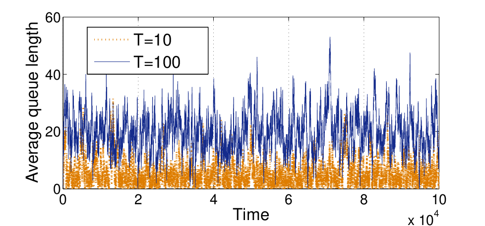
Over this system, we implement the proposed TT-frame queue-based index policy Q-Indexτ​(T,M−g⁡(τ)/2)\text{Q-Index}_{\tau}(T,M{-}g(\tau)/2), defined in section IV with τ=20\tau{=}20. We first consider fixed arrival rates λ1=λ2=0.25\lambda_{1}{=}\lambda_{2}{=}0.25 and implement the policies Q-Indexτ​(T,M−g⁡(τ)/2)\text{Q-Index}_{\tau}(T,M{-}g(\tau)/2) with frame lengths T=10T{=}10 and T=100T{=}100, respectively. The sample paths of the average queue length, i.e., (Q1​[t]+Q2​[t])/2\big(Q_{1}[t]+Q_{2}[t]\big)/2, are plotted in Fig. 4. It can be observed that, while the queues in both scenarios are stable, the variation of the queue evolution is notably higher when the frame size changes from 1010 to 100100. This is because, as the frame size increases, the frame-based algorithm obtains less frequent updates of the queue sizes. Therefore, within a frame, the algorithm can continue to serve a user even if its current queue length becomes small while neglecting the other user that has accumulated a large queue size, leading to a higher degree of queue length variation as well as average queue size. Correspondingly, higher delay and delay variation are expected as the frame size increases. For example, suppose the initial queue length of user 11 is empty, while the initial queue length for user 22 is nonempty. Then user 11 in the first frame will not be scheduled. Now after the first frame, the expected queue length of user 11 will be significantly larger for the case when T=100T=100 compared with the case when T=10T=10. Hence, at the second frame, the scheduler dedicates most of the resources to user 11. As a result, the expected queue length of the user 11 will go down after second frame, and the expected queue length of user 22 will grow. Both the expected change of queue lengths of user 11 and 22 will be much more significant when T=100T=100 compared with when T=10T=10. The process repeats in time and results in a higher degree of queue length variation when T=100T=100 as compared to T=10T=10.

Refer to caption
Fig. 4: Sample paths of queue evolution.

We next implement the aforementioned policy Q-Indexτ​(T,M−g⁡(τ)/2)\text{Q-Index}_{\tau}(T,M{-}g(\tau)/2) and evaluate the average queueing delay experienced by users as the arrival rates scale toward the boundary of the stability region, with varying frame length TT. For the two user system previously discussed, Fig. 5 examines the average queueing delay when the arrival rate vector (λ1,λ2)(\lambda_{1},\lambda_{2}) increases with λ1=λ2=λ\lambda_{1}{=}\lambda_{2}{=}\lambda. As can be observed in the figure, as the arrival rates grow toward the boundary of stability region, the queue length quickly blows up, resulting in steep increase of delay. The steep increase is because, as the arrival rates grow toward the boundary of stability region, the queue lengthes quickly blow up because they are becoming unstable, resulting in steep increase of average delay. Fig. 5 also show that, as the frame length grows, the average delay in the downlink network increases. This is, again, a consequence of infrequent update of queue length information at the scheduler.

Another interesting observation can be observed from Fig. 5. When we implement the proposed policy Q-Indexτ​(T,M−g⁡(τ)/2)\text{Q-Index}_{\tau}(T,M{-}g(\tau)/2) with the frame lengths TT growing from 99 to 100100, the system delay curves for different values of TT start to build up significantly at around the same value (i.e., around 0.290.29 which is on the boundary of the stability region). Note that we needed the frame size to be large enough to prove Proposition 1. However, in practice, the frame size TT may not need to be as large to guarantee queue stability. This numerical result, along with many other numerical evaluations we have conducted, indicates that the queues are stable under only moderate value of frame size in the proposed queue-based index policy.

Fig. 5 also plots the delay performance of a policy ϕN​o​F​b\phi^{NoFb} that ignores the channel memory, i.e., not using the channel state feedback. In each slot of this policy, a user ii with the largest multiplication of steady state transmission rate (i.e., bsib^{i}_{s}) and queue length qi​[t]q_{i}[t] is scheduled. The delay performance of maximum weight matching policy ϕM​W​M\phi^{MWM} is also plotted, where, in each slot tt, a user ii with the largest multiplication of belief value πi​[t]\pi^{i}[t] and queue length qi​[t]q_{i}[t] is scheduled. Fig. 5 further plots the delay performance of a naive policy ϕN​a​i​v​e​I​n​d\phi^{NaiveInd} where a user ii with the largest multiplication of index value Wi1​(πi​[t])W^{1}_{i}(\pi^{i}[t]) and queue length qi​[t]q_{i}[t] is scheduled. For all of these policies, the values of arrival rate λ\lambda where the queueing delay increases steeply are at a smaller value than our proposed policy, implying the sub-optimality of these policies. This is partly because these policies only schedule strictly MM users per slot, but our work is in the domain of a relaxed constraint of average number of scheduled users. The sub-optimality of policy ϕM​W​M\phi^{MWM} is also because it only exploits the channel condition in the instantaneous slot, i.e., πi​[t]\pi_{i}[t], but it does not consider exploring outdated channels. It is interesting to note that policy ϕM​W​M\phi^{MWM} and ϕN​a​i​v​e​I​n​d\phi^{NaiveInd} performs better than the policy that ignores channel state feedback, as the value of λ\lambda where steep increase of queueing delay occurs is much larger as compared to ϕN​o​F​b\phi^{NoFb}. This observation illustrates the throughput gains that can be achieved by using the channel state feedback.

Refer to caption
Fig. 5: Delay performance comparison when N=2N=2.

VI Conclusion

In this work, we have studied downlink scheduling problem over Markovian evolving ON/OFF fading channels and imperfect instantaneous channel state information. The scheduling decisions are made based on the single-bit ARQ-type feedback and the channel memory inherent in the Markovian channels. We propose a throughput-optimal policy that operates over time frames. In the proposed policy, the importance of scheduling a user is measured by a simple multiplication of the queue length and Whittle’s index value. Because of this property, the proposed policy has low-complexity per frame in the network size and the truncation level of the belief state space. Most notably, our policy does not suffer from the curse of dimensionality that is observed in earlier works in this context. Numerical evaluations show that significant throughput performance gains can be achieved by exploiting the channel memory, via the frame-based low-complexity queue-based index policy with moderate frame size. Future directions include considering larger state space model, and considering feedback mechanisms that collects CSI from unscheduled users, as well as more stringent instantaneous scheduling constraints. Another open direction is to consider adaptive power allocation with hybrid ARQ protocols (e.g., [9]), where the index value not only implies the attractiveness of scheduling a user, but also guides the power allocation across time.

Appendix A Proof of Lemma 1

The proof of the lemma is an extension of the proof of Proposition 1 in [16]. Consider the problem Ψ⁡(𝐫,M)\Psi(\mathbf{r},M) with weight vector 𝐫\mathbf{r}. The constraint (1) can be written in an equivalent form that requires at least N−MN-M channels to be passive on average, i.e.,

lim infT→∞1T​𝔼​[∑t=0T−1∑i=1N(1−aiϕ​[t])]≥N−M.\displaystyle\liminf_{T\rightarrow\infty}\frac{1}{T}\mathbb{E}\Big[\hskip-1.0pt\sum_{t=0}^{T-1}\sum_{i=1}^{N}(1{-}a_{i}^{\phi}[t])\Big]\geq N-M. (15)

Associating a Lagrange multiplier ω\omega to the constraint (15), we have the following Lagrangian function L⁡(ϕ,ω)L(\phi,\omega) for problem Ψ⁡(𝐫,M)\Psi(\mathbf{r},M),

L⁡(CLOSE\displaystyle L( OPENϕ,ω)=lim infT→∞1T​𝔼​[∑t=0T−1∑i=1Nri⋅πi​[t]⋅aiϕ​[t]]\displaystyle\phi,\omega){=}\liminf_{T\rightarrow\infty}\frac{1}{T}\mathbb{E}\Big[\sum_{t=0}^{T-1}\sum_{i=1}^{N}r_{i}{\cdot}\pi_{i}[t]{\cdot}a_{i}^{\phi}[t]\Big]
+ω⋅lim infT→∞1T𝔼[∑t=0T−1∑i=1N(1−aiϕ[t])]−ω⋅(N−M).\displaystyle{+}\omega{\cdot}\liminf_{T\rightarrow\infty}\frac{1}{T}\mathbb{E}\Big[\sum_{t=0}^{T-1}\sum_{i=1}^{N}(1{-}a^{\phi}_{i}[t])\Big]{-}\omega{\cdot}(N{-}M). (16)

The dual function D⁡(ω)D(\omega) is defined as D⁡(ω)=maxϕ∈Φ⁡L⁡(ϕ,ω)D(\omega)=\max_{\phi\in\Phi}L(\phi,\omega). Following the lines of proof in [16] we have

D⁡(ω)=∑i=1NUiri​(ω)+ω⁡(N−M).\displaystyle D(\omega)=\sum_{i=1}^{N}U_{i}^{r_{i}}(\omega)+\omega(N-M).

in which Uiri​(ω)U_{i}^{r_{i}}(\omega) is a ω\omega-subsidy problem under weight rir_{i},

Uiri​(ω)\displaystyle U_{i}^{r_{i}}(\omega) =maxϕ∈Φilim supT→∞1T𝔼[∑t=0T−1[ri⋅πi[t]⋅aiϕ[t]\displaystyle=\max_{\phi\in\Phi_{i}}\limsup_{T\rightarrow\infty}\frac{1}{T}\mathbb{E}\Big[\sum_{t=0}^{T-1}\big[r_{i}{\cdot}\pi_{i}[t]{\cdot}a^{\phi}_{i}[t]
+ω⋅(1−aiϕ[t])]],\displaystyle\hskip 108.405pt+\omega\cdot(1{-}a^{\phi}_{i}[t])\big]\Big], (17)

where Φi\Phi_{i} denotes the set of scheduling policies that activate and idle the user ii according to the observed channel history. In the above problem (17), for each channel ii at belief state πi\pi_{i}, it will receive a reward ri​πir_{i}\pi_{i} when it activates, otherwise it will receive a subsidy ω\omega for passivity. We let ℐiri​(ω)⊆ℬi\mathcal{I}^{r_{i}}_{i}(\omega)\subseteq\mathcal{B}_{i} be the set of belief states for which it is optimal to stay idle.

Under the unit weight ri=1r_{i}=1, it was shown in [18] that the problem is Whittle indexable, i.e., ℐi1​(ω)\mathcal{I}^{1}_{i}(\omega) monotonically increases from ∅\emptyset to ℬi\mathcal{B}_{i} as ω\omega increase from 00 to ∞\infty for each user ii. The Whittle’s index value Wi𝟏​(π)W_{i}^{\mathbf{1}}(\pi) is defined as the infimum subsidy value for which the belief state π\pi is at the boundary of ℐi1​(ω)\mathcal{I}^{1}_{i}(\omega), i.e.,

Wi𝟏​(π)=inf{ω:π∈ℐi1​(ω)}.\displaystyle W_{i}^{\mathbf{1}}(\pi)=\inf\{\omega:\pi\in\mathcal{I}^{1}_{i}(\omega)\}.

It follows from [16] that, for the ω\omega-subsidy problem under unit weight ri=1r_{i}=1, the optimal policy is to activate the user at time slot tt if Wi𝐫​(π)>ωW_{i}^{\mathbf{r}}(\pi)>\omega, and to stay idle if Wi𝐫​(π)<ωW_{i}^{\mathbf{r}}(\pi)<\omega, with tie breaking arbitrarily if Wi𝐫​(π)=ωW_{i}^{\mathbf{r}}(\pi)=\omega.

We next extend the optimal algorithm for the ω\omega-subsidy problem under unit weight to the general case with arbitrary non-negative weight rir_{i}. An equivalent form of Uiri​(ω)U_{i}^{r_{i}}(\omega) is as follows,

Uiri​(ω)\displaystyle U_{i}^{r_{i}}(\omega)
=\displaystyle\hskip-3.0pt{=} ri​max⁡lim supT→∞ϕ∈Φi⁡1T​𝔼​[∑t=0T−1[πi​[t]​aiϕ​[t]+ωri​(1−aiϕ​[t])]].\displaystyle r_{i}\max_{\phi\in\Phi_{i}}\limsup_{T\rightarrow\infty}\frac{1}{T}\mathbb{E}\Big[\sum_{t=0}^{T-1}\big[\pi_{i}[t]a^{\phi}_{i}[t]{+}\frac{\omega}{r_{i}}(1{-}a^{\phi}_{i}[t])\big]\Big]. (18)

Therefore, the optimal solution for the ω\omega-subsidy problem (17) with weight rir_{i} takes the same form as the optimal solution for the ω/ri\omega/r_{i}-subsidy problem with weight 11. Accordingly, the optimal solution takes the following form: a user ii is scheduled at slot tt if Wi𝐫​(πi​[t])>ω/riW_{i}^{\mathbf{r}}(\pi_{i}[t])>\omega/r_{i}, and stay idle if Wi𝐫​(π)<ω/riW_{i}^{\mathbf{r}}(\pi)<\omega/r_{i}, with tie breaking arbitrarily if Wi𝟏​(π)=ω/riW_{i}^{\mathbf{1}}(\pi)=\omega/r_{i}.

We define the 𝐫\mathbf{r}-weighted index value as Wi𝐫​(π)=ri⋅Wi𝟏​(π),π∈ℬi,i∈{1,⋯,N}W_{i}^{\mathbf{r}}(\pi)=r_{i}\cdot W_{i}^{\mathbf{1}}(\pi),\pi\in\mathcal{B}_{i},i\in\{1,\cdots,N\}. The optimal policy for the reward maximization problem in (18) is then to activate the user ii if Wi𝐫​(π)>ωW_{i}^{\mathbf{r}}(\pi)>\omega, and to stay idle if Wi𝐫​(π)<ωW_{i}^{\mathbf{r}}(\pi)<\omega, with tie breaking arbitrarily if Wi𝐫​(π)=ωW_{i}^{\mathbf{r}}(\pi)=\omega. Because of this threshold-based policy and arbitrary tie-breaking at the threshold, the dual function value D⁡(ω)D(\omega) can be achieved by the following threshold-based policy implemented over the 𝐫\mathbf{r}-weighted index values Wi𝐫​(π)W_{i}^{\mathbf{r}}(\pi): User ii is scheduled if Wi𝐫​(πi)>ωW^{\mathbf{r}}_{i}(\pi_{i}){>}\omega, or if Wi𝐫​(πi)=ωW^{\mathbf{r}}_{i}(\pi_{i}){=}\omega with i>ji{>}j. User ii stays idle if  Wi𝐫​(πi)<ωW^{\mathbf{r}}_{i}(\pi_{i}){<}\omega, or if Wi𝐫​(πi)=ωW^{\mathbf{r}}_{i}(\pi_{i}){=}\omega with i<ji{<}j. If Wi𝐫​(πi)=ωW^{\mathbf{r}}_{i}(\pi_{i}){=}\omega with i=ji{=}j, user ii is scheduled with probability ρ\rho.

Following the similar proof techniques of Lemma 11 in [16], by appropriately choosing the aforementioned parameters (j,ω,ρ)(j,\omega,\rho) to be (i∗,ω∗,ρ∗)(i^{*},\omega^{*},\rho^{*}) such that the constraint (1) on the average number of transmissions is strictly satisfied with equality, the corresponding policy is optimal for the problem Ψ⁡(𝐫,M)\Psi(\mathbf{r},M). Denoting such a policy as ϕ∗​(𝐫,M)\phi^{*}(\mathbf{r},M), the proposition is proven.

Appendix B Proof of Lemma 2

We next prove the Lemma for αjτ​(j,ω,ρ)\alpha^{\tau}_{j}\big(j,\omega,\rho\big).

Case (1). First consider αjτ​(j,Wj𝐫​(b0,hj),ρ)\alpha^{\tau}_{j}\big(j,W_{j}^{\mathbf{r}}(b^{j}_{0,h}),\rho\big) with h<τh<\tau. Hence user jj is scheduled if its belief value is above b0,hjb^{j}_{0,h}, or is scheduled with probability ρ\rho at belief value b0,hjb^{j}_{0,h}. According to the belief value evolution rule (2), in the next slot, its belief value will either be p11jp^{j}_{11} or p01jp^{j}_{01}, depending on the whether the revealed channel state is ‘00’ or ‘11’ at the end of the current slot. If the user’s belief value is below b0,hjb^{j}_{0,h}, it will not be scheduled and its belief value will move one step toward b0,h+1jb^{j}_{0,h+1}. Hence, in this case, the belief value evolution for user jj follows a Markov Chain over ℬjτ\mathcal{B}^{\tau}_{j}, as depicted in Fig. 6.

From Fig. 6, one can observe that the belief Markov chain is ergodic and the recurrent states are {b1,1j,b0,lj,l=1,⋯,h+1}\{b^{j}_{1,1},b^{j}_{0,l},l=1,\cdots,h+1\}. We denote the stationary probability of belief value being πj\pi_{j} as ζj​(πj),πj∈ℬjτ\zeta_{j}(\pi_{j}),\pi_{j}\in\mathcal{B}^{\tau}_{j}. The global balance equations are

ρ⁡(1−b0,hj)​ζj​(b0,hj)+ζj​(b0,h+1j)​(1−b0,h+1j)\displaystyle\rho(1{-}b^{j}_{0,h})\zeta_{j}(b^{j}_{0,h}){+}\zeta_{j}(b^{j}_{0,h{+}1})(1{-}b^{j}_{0,h{+}1})
+b1,1j​(1−CLOSE\displaystyle{+}b^{j}_{1,1}(1{-} OPENp11j)=ζj​(b0,1j)\displaystyle p^{j}_{11})=\zeta_{j}(b^{j}_{0,1})
ζj​(b0,1j)=ζj​(b0,2j)=,⋯,=ζj\displaystyle\zeta_{j}(b^{j}_{0,1})=\zeta_{j}(b^{j}_{0,2})=,\cdots,=\zeta_{j} (b0,hj)\displaystyle(b^{j}_{0,h})
(1−ρ)​ζj​(b0,hj)=ζj​(b0,h+1jCLOSE\displaystyle(1-\rho)\zeta_{j}(b^{j}_{0,h})=\zeta_{j}(b^{j}_{0,h+1} )\displaystyle)
ρ​ζj​(b0,hj)+ζj​(b0,h+1j)=(1−p11j)\displaystyle\rho\zeta_{j}(b^{j}_{0,h})+\zeta_{j}(b^{j}_{0,h+1})=(1-p^{j}_{11}) ζj​(b1,1j)\displaystyle\zeta_{j}(b^{j}_{1,1})

From the balance equations, we can calculate the expression of the stationary probability as follows,

ζj​(πj)\displaystyle\zeta_{j}(\pi_{j})
=\displaystyle={\hskip-5.0pt} {1−p11jρ​b0,hj+(1−ρ)​b0,h+1j+(1−p11j)​(h+1−ρ)​if πj=b0,kj, k≤h;(1−ρ)​(1−p11j)ρ​b0,hj+(1−ρ)​b0,h+1j+(1−p11j)​(h+1−ρ)​if πj=b0,h+1j;b0,h+1j+ρ⁡(b0,hj−b0,h+1j)ρ​b0,hj+(1−ρ)​b0,h+1j+(1−p11j)​(h+1−ρ)​if πj=b1,1j;0​ otherwise.\displaystyle\begin{cases}&\frac{1-p^{j}_{11}}{\rho b^{j}_{0,h}{+}(1{-}\rho)b^{j}_{0,h\hskip-1.0pt{+}\hskip-1.0pt1}{+}(1\hskip-1.0pt{-}\hskip-1.0ptp^{j}_{11})(h{+}1{-}\rho)}\text{if $\pi_{j}{=}b^{j}_{0,k}$, $k\leq h$;}\\ &\frac{(1-\rho)(1-p^{j}_{11})}{\rho b^{j}_{0,h}{+}(1{-}\rho)b^{j}_{0,h\hskip-1.0pt{+}\hskip-1.0pt1}{+}(1\hskip-1.0pt{-}\hskip-1.0ptp^{j}_{11})(h{+}1{-}\rho)}\text{if $\pi_{j}{=}b^{j}_{0,h+1}$;}\\ &\frac{b^{j}_{0,h+1}+\rho(b^{j}_{0,h}-b^{j}_{0,h+1})}{\rho b^{j}_{0,h}{+}(1{-}\rho)b^{j}_{0,h\hskip-1.0pt{+}\hskip-1.0pt1}{+}(1\hskip-1.0pt{-}\hskip-1.0ptp^{j}_{11})(h{+}1{-}\rho)}\text{if $\pi_{j}{=}b^{j}_{1,1}$;}\\ &0\text{\hskip 127.9182ptotherwise.}\end{cases}

Hence, the expected fraction of time transmitting to user jj is

αjτ​(j,Wj𝐫​(b0,hj),ρ)\displaystyle\alpha^{\tau}_{j}\big(j,W_{j}^{\mathbf{r}}(b^{j}_{0,h}),\rho\big) =ρ​ζj​(b0,hj)+ζj​(b0,h+1j)+ζj​(b1,1j)\displaystyle=\rho\zeta_{j}(b^{j}_{0,h})+\zeta_{j}(b^{j}_{0,h+1})+\zeta_{j}(b^{j}_{1,1})
=ρ⁡(b0,hj−b0,h+1j)+1−p11j+b0,h+1jρ​b0,hj+(1−ρ)​b0,h+1j+(1−p11j)​(h+1−ρ),\displaystyle=\frac{\rho(b^{j}_{0,h}-b^{j}_{0,h+1})+1-p^{j}_{11}+b^{j}_{0,h{+}1}}{\rho b^{j}_{0,h}{+}(1{-}\rho)b^{j}_{0,h\hskip-1.0pt{+}\hskip-1.0pt1}{+}(1\hskip-1.0pt{-}\hskip-1.0ptp^{j}_{11})(h{+}1{-}\rho)},

as given in Lemma 2(i). To prove part (ii), we consider its reciprocal, i.e.,

[αjτ​(j,Wj𝐫​(b0,hj),ρ)]−1\displaystyle[\alpha^{\tau}_{j}\big(j,W_{j}^{\mathbf{r}}(b^{j}_{0,h}),\rho\big)]^{-1}
=\displaystyle= 1+(1−p11j)​(h−ρ)ρ⁡(b0,hj−b0,h+1j)+1−p11j+b0,h+1j\displaystyle 1+\frac{(1-p^{j}_{11})(h-\rho)}{\rho(b^{j}_{0,h}-b^{j}_{0,h+1})+1-p^{j}_{11}+b^{j}_{0,h{+}1}}
=\displaystyle= 1+1−p11jb0,h+1j−b0,hj​[1−1−p11j+b0,h+1j+h⁡(b0,hj−b0,h+1j)ρ⁡(b0,hj−b0,h+1j)+b0,h+1j+(1−p11j)].\displaystyle 1{+}\frac{1-p^{j}_{11}}{b_{0,h{+}1}^{j}{-}b_{0,h}^{j}}\Big[1{-}\frac{1-p^{j}_{11}+b_{0,h+1}^{j}+h(b_{0,h}^{j}-b_{0,h+1}^{j})}{\rho(b_{0,h}^{j}{-}b_{0,h{+}1}^{j})+b_{0,h+1}^{j}+(1-p^{j}_{11})}\Big]. (19)
Refer to caption
Fig. 6: Belief value transition in steady state when ω=Wj𝐫​(b0,hj)\omega{=}W_{j}^{\mathbf{r}}(b^{j}_{0,h}).

Considering the numerator inside the parenthesis of (19), we have

1−p11j+b0,h+1j+h⁡(b0,hj−b0,h+1j)\displaystyle 1-p^{j}_{11}+b_{0,h+1}^{j}+h(b_{0,h}^{j}-b_{0,h+1}^{j})
≥\displaystyle\geq 1−p11j+b0,h+1j+(h+1)​(b0,hj−b0,h+1j)≥0,\displaystyle 1-p^{j}_{11}+b_{0,h+1}^{j}+(h+1)(b_{0,h}^{j}-b_{0,h+1}^{j})\geq 0,

where the last inequality is from (51). Noting that the denominator inside the parenthesis of (19) strictly decreases with ρ\rho, hence [αjτ​(j,Wj𝐫​(b0,hj),ρ)]−1[\alpha^{\tau}_{j}\big(j,W_{j}^{\mathbf{r}}(b^{j}_{0,h}),\rho\big)]^{-1} strictly decreases with ρ\rho. Therefore αjτ​(j,Wj𝐫​(πj),ρ)\alpha^{\tau}_{j}\big(j,W_{j}^{\mathbf{r}}(\pi_{j}),\rho\big) strictly decreases with ρ\rho for πj\pi_{j} for πj∈{b0,1j,b0,2j,⋯,b0,τ−1j}\pi_{j}\in\{b^{j}_{0,1},b^{j}_{0,2},\cdots,b^{j}_{0,\tau-1}\}

Since for h+1<τh{+}1{<}\tau, αjτ​(j,Wj𝐫​(b0,hj),0)=αjτ​(j,Wj𝐫​(b0,h+1j),1)\alpha^{\tau}_{j}(j,W_{j}^{\mathbf{r}}(b^{j}_{0,h}),0)=\alpha^{\tau}_{j}(j,W_{j}^{\mathbf{r}}(b^{j}_{0,h+1}),1), we have,

αjτ​(j,Wj𝐫​(b0,h+1j),ρ)\displaystyle\alpha^{\tau}_{j}(j,W_{j}^{\mathbf{r}}(b^{j}_{0,h+1}),\rho) ≤αjτ​(j,Wj𝐫​(b0,h+1j),1)\displaystyle\leq\alpha^{\tau}_{j}(j,W_{j}^{\mathbf{r}}(b^{j}_{0,h+1}),1)
=αjτ​(j,Wj𝐫​(b0,hj),0)\displaystyle=\alpha^{\tau}_{j}(j,W_{j}^{\mathbf{r}}(b^{j}_{0,h}),0)
≤αjτ​(j,Wj𝐫​(b0,hj),ρ).\displaystyle\leq\alpha^{\tau}_{j}(j,W_{j}^{\mathbf{r}}(b^{j}_{0,h}),\rho).

Therefore, for fixed ρ\rho, αjτ​(j,Wj𝐫​(πj),ρ){\alpha}^{\tau}_{j}(j,W_{j}^{\mathbf{r}}(\pi_{j}),\rho) strictly decreases with πj\pi_{j} for πj∈{b0,1j,b0,2j,⋯,b0,τ−1j}\pi_{j}\in\{b^{j}_{0,1},b^{j}_{0,2},\cdots,b^{j}_{0,\tau-1}\}.

Case (2). Next consider αjτ​(j,Wj𝐫​(bτj),ρ)\alpha^{\tau}_{j}\big(j,W_{j}^{\mathbf{r}}(b^{j}_{\tau}),\rho\big). We can perform a similar analysis as in case (1) to obtain

αjτ​(j,Wj𝐫​(b0,τj),ρ)\displaystyle\alpha^{\tau}_{j}\big(j,W_{j}^{\mathbf{r}}(b^{j}_{0,\tau}),\rho\big) =ρ⁡(b0,τj−bsj)+1−p11j+bsjρ​b0,τj+(1−ρ)​bsj+(1−p11j)​(τ+1−ρ),\displaystyle=\frac{\rho(b^{j}_{0,\tau}-b^{j}_{s})+1-p^{j}_{11}+b^{j}_{s}}{\rho b^{j}_{0,\tau}{+}(1{-}\rho)b^{j}_{s}{+}(1\hskip-1.0pt{-}\hskip-1.0ptp^{j}_{11})(\tau{+}1{-}\rho)},
[αjτ​(j,Wj𝐫​(b0,τj),ρ)]−1\displaystyle[\alpha^{\tau}_{j}\big(j,W_{j}^{\mathbf{r}}(b^{j}_{0,\tau}),\rho\big)]^{-1}\hskip-10.0pt
=1+1−p11jbsj−b0,τj​[1−1−p11j+bsj+τ⁡(b0,τj−bsj)ρ⁡(b0,τj−bsj)+bsj+(1−p11j)].\displaystyle\hskip-72.26999pt=1{+}\frac{1-p^{j}_{11}}{b_{s}^{j}{-}b_{0,\tau}^{j}}\Big[1{-}\frac{1-p^{j}_{11}+b_{s}^{j}+\tau(b_{0,\tau}^{j}-b_{s}^{j})}{\rho(b_{0,\tau}^{j}{-}b_{s}^{j})+b_{s}^{j}+(1-p^{j}_{11})}\Big]. (20)

When τ>τ0\tau>\tau_{0}, it can be derived that the numerator 1−p11j+bsj+τ⁡(b0,τj−bsj)1-p^{j}_{11}+b_{s}^{j}+\tau(b_{0,\tau}^{j}-b_{s}^{j}) inside (20) is positive. Therefore αjτ​(j,Wj𝐫​(b0,τj),ρ)\alpha^{\tau}_{j}\big(j,W_{j}^{\mathbf{r}}(b^{j}_{0,\tau}),\rho\big) strictly increases with ρ\rho. Similar to Case (1), we have

αjτ​(j,Wj𝐫​(b0,τj),ρ)\displaystyle\alpha^{\tau}_{j}(j,W_{j}^{\mathbf{r}}(b^{j}_{0,\tau}),\rho) ≤αjτ​(j,Wj𝐫​(b0,τj),1)=αjτ​(j,Wj𝐫​(b0,τ−1j),0)\displaystyle\leq\alpha^{\tau}_{j}(j,W_{j}^{\mathbf{r}}(b^{j}_{0,\tau}),1)=\alpha^{\tau}_{j}(j,W_{j}^{\mathbf{r}}(b^{j}_{0,\tau-1}),0)
≤αjτ​(j,Wj𝐫​(b0,τ−1j),ρ).\displaystyle\leq\alpha^{\tau}_{j}(j,W_{j}^{\mathbf{r}}(b^{j}_{0,\tau-1}),\rho).

Case (3). Consider αjτ​(j,Wj𝐫​(bsj),ρ)\alpha^{\tau}_{j}\big(j,W_{j}^{\mathbf{r}}(b^{j}_{s}),\rho\big). Similar to Case (1), we obtain,

αjτ​(j,Wj𝐫​(bsj),ρ)\displaystyle\alpha^{\tau}_{j}\big(j,W_{j}^{\mathbf{r}}(b^{j}_{s}),\rho\big) =ρ⁡(1−p11j+bsj)(1+τ​ρ)​(1−p11j)+ρ​bsj.\displaystyle{=}\frac{\rho(1-p^{j}_{11}+b^{j}_{s})}{(1+\tau\rho)(1-p^{j}_{11})+\rho b^{j}_{s}}.

Taking the reciprocal we have

[αjτ​(j,Wj𝐫​(bsj),ρ)]−1\displaystyle[\alpha^{\tau}_{j}\big(j,W_{j}^{\mathbf{r}}(b^{j}_{s}),\rho\big)]^{-1} =11−p11j+bsj​((1−p11j)​(τ+1ρ)+bsj),\displaystyle=\frac{1}{1-p^{j}_{11}+b^{j}_{s}}\Big((1-p^{j}_{11})(\tau+\frac{1}{\rho})+b^{j}_{s}\Big),

which strictly decreases with ρ\rho. Hence αjτ​(j,Wj𝐫​(bsj),ρ)\alpha^{\tau}_{j}\big(j,W_{j}^{\mathbf{r}}(b^{j}_{s}),\rho\big) strictly increases with ρ\rho. We also have

αjτ​(j,Wj𝐫​(bsj),ρ)\displaystyle\alpha^{\tau}_{j}(j,W_{j}^{\mathbf{r}}(b^{j}_{s}),\rho) ≤αjτ​(j,Wj𝐫​(bsj),1)=αjτ​(j,Wj𝐫​(b0,τj),0)\displaystyle\leq\alpha^{\tau}_{j}(j,W_{j}^{\mathbf{r}}(b^{j}_{s}),1)=\alpha^{\tau}_{j}(j,W_{j}^{\mathbf{r}}(b^{j}_{0,\tau}),0)
≤αjτ​(j,Wj𝐫​(b0,τj),ρ).\displaystyle\leq\alpha^{\tau}_{j}(j,W_{j}^{\mathbf{r}}(b^{j}_{0,\tau}),\rho).

From Case (1)-(3), the lemma is established for αjτ​(j,Wj𝐫​(b0,hj),ρ)\alpha^{\tau}_{j}\big(j,W_{j}^{\mathbf{r}}(b^{j}_{0,h}),\rho\big). Noting that for user i≠ji\neq j, there is no randomization associated with scheduling. Hence, the above derivation for αjτ​(j,Wj𝐫​(b0,hj),ρ)\alpha^{\tau}_{j}\big(j,W_{j}^{\mathbf{r}}(b^{j}_{0,h}),\rho\big) naturally extends to αiτ​(j,Wi𝐫​(b0,hj),ρ)\alpha^{\tau}_{i}\big(j,W_{i}^{\mathbf{r}}(b^{j}_{0,h}),\rho\big). The only change is there is no longer randomization involved. Details are hence neglected here.

Appendix C Proof of Lemma 3

C-A Proof outline

We establish the proof by first proving lemma 4 that bounds the difference of weighted sum-throughput between policies with different threshold parameters, with respective to the difference between expected fraction of transmission time to each user. We then prove the lemma under two cases, i.e., whether ω∗<Wi𝐫​(b0,τi)\omega^{*}<W^{\mathbf{r}}_{i}(b^{i}_{0,\tau}) for all user ii. The first case is uncomplicated to prove. For the second case, we first prove a useful fact that only one of the three cases holds: ωτ>ω∗\omega_{\tau}>\omega^{*}, or ωτ=ω∗\omega_{\tau}=\omega^{*} with ρτ<ρ∗\rho_{\tau}<\rho^{*} and iτ=i∗i_{\tau}=i^{*}, or ωτ=ω∗\omega_{\tau}=\omega^{*} with iτ>i∗i_{\tau}>i^{*}. Based on these cases, we can bound the difference between expected fraction of time transmitting to different users. We then use Lemma 4 to finish the proof.

C-B Notations

Recall that, in the untruncated state space, the optimal policy ϕ∗​(𝐫,M)\phi^{*}(\mathbf{r},M) corresponds to the parameters (i∗,ω∗,ρ∗)(i^{*},\omega^{*},\rho^{*}). Also recall that, in the truncated state space, the policy ϕτ​(𝐫,M)\phi_{\tau}(\mathbf{r},M) corresponds to the parameter (iτ,ωτ,ρτ)(i_{\tau},\omega_{\tau},\rho_{\tau}).

Over the actual untruncated model, consider the following policy denoted as ϕj,ω,ρu​n​t​r​u​n​c\phi^{untrunc}_{j,\omega,\rho} with the parameters (j,ω,ρ)(j,\omega,\rho): User ii is scheduled if Wi𝐫​(πi​[t])>ωW^{\mathbf{r}}_{i}(\pi_{i}[t]){>}\omega, or if Wi𝐫​(πi​[t])=ω∗W^{\mathbf{r}}_{i}(\pi_{i}[t]){=}\omega^{*} with i>ji{>}j. User ii stays idle if Wi𝐫​(πiτ​[t])<ωW^{\mathbf{r}}_{i}(\pi_{i}^{\tau}[t]){<}\omega, or if Wi𝐫​(πiτ​[t])=ω∗W^{\mathbf{r}}_{i}(\pi_{i}^{\tau}[t]){=}\omega^{*} with i<ji{<}j. If Wi𝐫​(πiτ​[t])=ωW^{\mathbf{r}}_{i}(\pi_{i}^{\tau}[t]){=}\omega with i=ji{=}j, it is scheduled with probability ρ\rho. In this model, similar to (8), we let αi​(j,ω,ρ){\alpha}_{i}(j,\omega,\rho) denote the long-term expected fraction of time transmitting to user ii under policy ϕj,ω,ρu​n​t​r​u​n​c\phi^{untrunc}_{j,\omega,\rho}, i.e.,

αi​(j,ω,ρ)=lim supT→∞1T​𝔼​[∑t=0T−1aiϕj,ω,ρu​n​t​r​u​n​c​[t]].\displaystyle{\alpha}_{i}(j,\omega,\rho)=\limsup_{T\rightarrow\infty}\frac{1}{T}\mathbb{E}\Big[\sum_{t=0}^{T-1}a_{i}^{\phi^{untrunc}_{j,\omega,\rho}}[t]\Big]. (21)

The closed-form expression of αi​(j,ω,ρ){\alpha}_{i}(j,\omega,\rho) can be calculated from the same technique we used to prove Lemma 2 as follows.

αi​(j,ω,ρ)\displaystyle{\alpha}_{i}(j,\omega,\rho)
=\displaystyle={\hskip-5.0pt} {ρ⁡(b0,hi−b0,h+1i)+1−p11i+b0,h+1iρ​b0,hi+(1−ρ)​b0,h+1i+(1−p11i)​(h+1−ρ)if ω=Wi𝐫​(b0,hi),i=j;1−p11i+b0,h+1ib0,h+1i+(1−p11i)​(h+1)if ω=Wi𝐫​(b0,hi), i<j1−p11i+b0,hib0,hi+(1−p11i)​hif ω=Wi𝐫​(b0,hi), i>j;or if Wi𝐫​(b0,h−1i)<ω<Wi𝐫​(b0,hi), i≠j0if ω≥Wi𝐫​(bsi).\displaystyle\begin{cases}\frac{\rho(b^{i}_{0,h}-b^{i}_{0,h+1})+1-p^{i}_{11}+b^{i}_{0,h{+}1}}{\rho b^{i}_{0,h}{+}(1{-}\rho)b^{i}_{0,h\hskip-1.0pt{+}\hskip-1.0pt1}{+}(1\hskip-1.0pt{-}\hskip-1.0ptp^{i}_{11})(h{+}1{-}\rho)}&\text{if $\omega{=}W^{\mathbf{r}}_{i}(b^{i}_{0,h}),i{=}j$;}\\ \frac{1-p^{i}_{11}+b^{i}_{0,h{+}1}}{b^{i}_{0,h{+}1}{+}(1{-}p^{i}_{11})(h{+}1)}&\text{if $\omega{=}W^{\mathbf{r}}_{i}(b^{i}_{0,h})$, $i{<}j$}\\ \frac{1-p^{i}_{11}+b^{i}_{0,h}}{b^{i}_{0,h}{+}(1{-}p^{i}_{11})h}&\text{if $\omega{=}W^{\mathbf{r}}_{i}(b^{i}_{0,h})$, $i>j$;}\\ &\text{\hskip-68.65627ptor if $W^{\mathbf{r}}_{i}(b^{i}_{0,h{-}1}){<}\omega{<}W^{\mathbf{r}}_{i}(b^{i}_{0,h})$, $i\neq j$}\\ 0&\text{if $\omega{\geq}W^{\mathbf{r}}_{i}(b^{i}_{s})$.}\end{cases} (22)

We also let υi​(j,ω,ρ)\upsilon_{i}(j,\omega,\rho) denote the long-term expected transmission rate to user ii, i.e.,

υi​(j,ω,ρ)=lim infT→∞1T​𝔼​[∑t=0T−1ri⋅πi​[t]⋅aiϕj,ω,ρu​n​t​r​u​n​c​[t]],\displaystyle\upsilon_{i}(j,\omega,\rho)=\liminf_{T\rightarrow\infty}\frac{1}{T}\mathbb{E}\Big[\sum_{t=0}^{T-1}r_{i}\cdot\pi_{i}[t]\cdot a_{i}^{\phi^{untrunc}_{j,\omega,\rho}}[t]\Big], (23)

Over the truncated model, correspondingly, we let υiτ​(j,ω,ρ)\upsilon_{i}^{\tau}(j,\omega,\rho) denote the long-term expected transmission rate to user ii under policy ϕj,ω,ρt​r​u​n​c\phi^{trunc}_{j,\omega,\rho} defined in section III-D, i.e.,

υiτ​(j,ω,ρ)=lim infT→∞1T​𝔼​[∑t=0T−1ri⋅πiτ​[t]⋅aiϕj,ω,ρt​r​u​n​c​[t]].\displaystyle\upsilon_{i}^{\tau}(j,\omega,\rho)=\liminf_{T\rightarrow\infty}\frac{1}{T}\mathbb{E}\Big[\sum_{t=0}^{T-1}r_{i}\cdot\pi_{i}^{\tau}[t]\cdot a_{i}^{\phi^{trunc}_{j,\omega,\rho}}[t]\Big]. (24)

Using techniques similar to the proof of Lemma 2, we can derive the analytical expressions of υi​(j,ω,ρ)\upsilon_{i}(j,\omega,\rho) and υiτ​(j,ω,ρ)\upsilon_{i}^{\tau}(j,\omega,\rho) as follows,

υi​(j,ω,ρ)=\displaystyle{\upsilon}_{i}(j,\omega,\rho)=
{ri⋅ρ​b0,hi+(1−ρ)​b0,h+1iρ​b0,hi+(1−ρ)​b0,h+1i+(1−p11i)​(h+1−ρ)if ω=Wi𝐫​(b0,hi), i=jri⋅b0,h+1ib0,h+1i+(1−p11i)​(h+1)if ω=Wi𝐫​(b0,hi), i<jri⋅b0,hib0,hi+(1−p11i)​hif ω=Wi𝐫​(b0,hi), i>jor if Wi𝐫​(b0,h−1i)<ω<Wi𝐫​(b0,hi), i≠j0if ω≥Wi𝐫​(bsi).\displaystyle\hskip-3.0pt\begin{cases}r_{i}{\cdot}\frac{\rho b_{0,h}^{i}+(1-\rho)b_{0,h+1}^{i}}{\rho b_{0,h}^{i}{+}(1{-}\rho)b_{0,h{+}1}^{i}{+}(1{-}p^{i}_{11})(h{+}1{-}\rho)}&\text{\hskip-5.0ptif $\omega{=}W_{i}^{\mathbf{r}}(b^{i}_{0,h})$, $i{=}j$}\\ r_{i}{\cdot}\frac{b_{0,h+1}^{i}}{b_{0,h{+}1}^{i}{+}(1{-}p^{i}_{11})(h{+}1)}&\text{\hskip-5.0ptif $\omega{=}W^{\mathbf{r}}_{i}(b^{i}_{0,h})$, $i{<}j$}\\ r_{i}{\cdot}\frac{b_{0,h}^{i}}{b_{0,h}^{i}{+}(1{-}p^{i}_{11})h}&\text{\hskip-5.0ptif $\omega{=}W_{i}^{\mathbf{r}}(b^{i}_{0,h})$, $i{>}j$}\\ &\text{\hskip-79.49744ptor if $W^{\mathbf{r}}_{i}(b^{i}_{0,h{-}1}){<}\omega{<}W^{\mathbf{r}}_{i}(b^{i}_{0,h})$, $i\neq j$}\\ 0&\text{\hskip-5.0ptif $\omega{\geq}W_{i}^{\mathbf{r}}(b^{i}_{s})$.}\end{cases} (25)

The expression of υjτ​(j,ω,ρ){\upsilon}^{\tau}_{j}(j,\omega,\rho) is given as follows,

υjτ​(j,ω,ρ)=\displaystyle{\upsilon}^{\tau}_{j}(j,\omega,\rho)=
{rj⋅ρ​b0,hj+(1−ρ)​b0,h+1jρ​b0,hj+(1−ρ)​b0,h+1j+(1−p11j)​(h+1−ρ)if h<τ, ω=Wj𝐫​(b0,hj);rj⋅ρ​b0,τj+(1−ρ)​bsjρ​b0,τj+(1−ρ)​bsj+(1−p11j)​(τ+1−ρ)if ω=Wj𝐫​(b0,τj);rj⋅ρ​bsj(1+τ​ρ)​(1−p11j)+ρ​bsjif ω=Wj𝐫​(bsj);0if ω>Wj𝐫​(bsj).\displaystyle\hskip-3.0pt\begin{cases}r_{j}{\cdot}\frac{\rho b_{0,h}^{j}+(1-\rho)b_{0,h+1}^{j}}{\rho b_{0,h}^{j}{+}(1{-}\rho)b_{0,h{+}1}^{j}{+}(1{-}p^{j}_{11})(h{+}1{-}\rho)}&\text{if $h{<}\tau$, $\omega{=}W^{\mathbf{r}}_{j}(b^{j}_{0,h})$;}\\ r_{j}{\cdot}\frac{\rho b_{0,\tau}^{j}+(1-\rho)b_{s}^{j}}{\rho b_{0,\tau}^{j}{+}(1{-}\rho)b_{s}^{j}{+}(1{-}p^{j}_{11})(\tau{+}1{-}\rho)}&\text{if $\omega{=}W_{j}^{\mathbf{r}}(b^{j}_{0,\tau})$;}\\ r_{j}{\cdot}\frac{\rho b^{j}_{s}}{(1+\tau\rho)(1{-}p^{j}_{11}){+}\rho b^{j}_{s}}&\text{if $\omega{=}W_{j}^{\mathbf{r}}(b^{j}_{s})$;}\\ 0&\text{if $\omega{>}W_{j}^{\mathbf{r}}(b^{j}_{s})$.}\end{cases} (26)

The expression of υiτ​(j,ω,ρ){\upsilon}^{\tau}_{i}(j,\omega,\rho), i≠ji\neq j is expressed as follows.

υiτ​(j,ω,ρ)=\displaystyle{\upsilon}^{\tau}_{i}(j,\omega,\rho)=
{ri⋅b0,h+1ib0,h+1i+(1−p11i)​(h+1)if h<τ, ω=Wi𝐫​(b0,hi), i<jri⋅b0,hib0,hi+(1−p11i)​hif h≤τ, ω=Wi𝐫​(b0,hi), i>j;or if h≤τ,Wi𝐫​(b0,h−1i)<ω<Wi𝐫​(b0,hi)ri⋅bsi(1+τ)​(1−p11i)+bsiif ω=Wi𝐫​(b0,τi), i<j;or if ω=Wi𝐫​(bsi), i>j0if ω=Wi𝐫​(bsi), i<jor if ω>Wi𝐫​(bsi).\displaystyle\hskip-3.0pt\begin{cases}r_{i}{\cdot}\frac{b_{0,h+1}^{i}}{b_{0,h{+}1}^{i}{+}(1{-}p^{i}_{11})(h{+}1)}&\text{if $h{<}\tau$, $\omega{=}W^{\mathbf{r}}_{i}(b^{i}_{0,h})$, $i{<}j$}\\ r_{i}{\cdot}\frac{b_{0,h}^{i}}{b_{0,h}^{i}{+}(1{-}p^{i}_{11})h}&\text{if $h{\leq}\tau$, $\omega{=}W^{\mathbf{r}}_{i}(b^{i}_{0,h})$, $i>j$;}\\ &\text{or if $h{\leq}\tau$,$W^{\mathbf{r}}_{i}(b^{i}_{0,h{-}1}){<}\omega{<}W^{\mathbf{r}}_{i}(b^{i}_{0,h})$}\\ r_{i}{\cdot}\frac{b^{i}_{s}}{(1+\tau)(1{-}p^{i}_{11}){+}b^{i}_{s}}&\text{if $\omega{=}W^{\mathbf{r}}_{i}(b^{i}_{0,\tau})$, $i<j$;}\\ &\text{or if $\omega{=}W^{\mathbf{r}}_{i}(b^{i}_{s})$, $i>j$}\\ 0&\text{if $\omega{=}W^{\mathbf{r}}_{i}(b^{i}_{s})$, $i<j$}\\ &\text{or if $\omega{>}W^{\mathbf{r}}_{i}(b^{i}_{s})$.}\end{cases} (27)

C-C Proof of Lemma 3

We first prove the following lemma that provides properties of αiτ​(j,ω,ρ){\alpha}^{\tau}_{i}(j,\omega,\rho) and υiτ​(j,ω,ρ){\upsilon}^{\tau}_{i}(j,\omega,\rho).

Lemma 4.

For a user ii, if τ≥τ0\tau\geq\tau_{0}, we have

(i) For fixed πj∈{b0,1j,b0,2j,⋯,b0,τj,bsj}\pi_{j}{\in}\{b^{j}_{0,1},b^{j}_{0,2},{\cdots},b^{j}_{0,\tau},b^{j}_{s}\}, υjτ​(j,Wj𝐫​(πi),ρ){\upsilon}^{\tau}_{j}(j,W_{j}^{\mathbf{r}}(\pi_{i}),\rho) strictly increases with ρ\rho. For fixed ρ\rho, υiτ​(j,Wi𝐫​(πi),ρ){\upsilon}^{\tau}_{i}(j,W_{i}^{\mathbf{r}}(\pi_{i}),\rho) strictly decreases with πi\pi_{i} for πi∈{b0,1i,b0,2i,⋯,b0,τi,bsi}\pi_{i}\in\{b^{i}_{0,1},b^{i}_{0,2},\cdots,b^{i}_{0,\tau},b^{i}_{s}\} and all ii;

(ii) for any two sets of parameter {j1,ω1,ρ1}\{j_{1},\omega_{1},\rho_{1}\} and {j2,ω2,ρ2}\{j_{2},\omega_{2},\rho_{2}\},

|υiτ​(j1,ω1,ρ1)−υiτ​(j2,ω2,ρ2)|\displaystyle\Big|\hskip 2.0pt{\upsilon}^{\tau}_{i}(j_{1},\omega_{1},\rho_{1})-{\upsilon}^{\tau}_{i}(j_{2},\omega_{2},\rho_{2})\Big|
≤\displaystyle\leq ri⋅|αiτ​(j1,ω1,ρ1)−αiτ​(j2,ω2,ρ2)|.\displaystyle r_{i}\cdot\Big|\hskip 2.0pt{\alpha}^{\tau}_{i}(j_{1},\omega_{1},\rho_{1})-{\alpha}^{\tau}_{i}(j_{2},\omega_{2},\rho_{2})\Big|.

Proof: See Appendix E. ■\hfill\blacksquare

Note that we need τ≥τ0\tau\geq\tau_{0} for the proof to hold. Since the untruncated state space is in the asymptotic regime of the truncated scenario when τ→∞\tau{\rightarrow}\infty, a straightforward extension of properties of αiτ​(j,ω,ρ){\alpha}^{\tau}_{i}(j,\omega,\rho) and υiτ​(j,ω,ρ){\upsilon}^{\tau}_{i}(j,\omega,\rho) in Lemma 2 and Lemma 4 to αi​(j,ω,ρ){\alpha}_{i}(j,\omega,\rho) and υi​(j,ω,ρ){\upsilon}_{i}(j,\omega,\rho) in the untruncated scenario leads to the next Lemma.

Lemma 5.

For a user ii, if τ≥τ0\tau\geq\tau_{0}, we have

(i) For fixed πj∈{b0,1j,b0,2j,⋯,b0,τj,bsj}\pi_{j}{\in}\{b^{j}_{0,1},b^{j}_{0,2},{\cdots},b^{j}_{0,\tau},b^{j}_{s}\}, υj​(j,Wj𝐫​(πi),ρ){\upsilon}_{j}(j,W_{j}^{\mathbf{r}}(\pi_{i}),\rho) and αi​(j,Wi𝐫​(πi),ρ){\alpha}_{i}(j,W_{i}^{\mathbf{r}}(\pi_{i}),\rho) strictly increase with ρ\rho. For fixed ρ\rho, υi​(j,Wi𝐫​(πi),ρ){\upsilon}_{i}(j,W_{i}^{\mathbf{r}}(\pi_{i}),\rho) and αi​(j,Wi𝐫​(πi),ρ){\alpha}_{i}(j,W_{i}^{\mathbf{r}}(\pi_{i}),\rho) strictly decrease with πi\pi_{i} for πi∈{b0,1i,b0,2i,⋯,b0,τi,bsi}\pi_{i}\in\{b^{i}_{0,1},b^{i}_{0,2},\cdots,b^{i}_{0,\tau},b^{i}_{s}\};

(ii) for any two sets of parameters {j1,ω1,ρ1}\{j_{1},\omega_{1},\rho_{1}\} and {j2,ω2,ρ2}\{j_{2},\omega_{2},\rho_{2}\},

|υi​(j1,ω1,ρ1)−υi​(j2,ω2,ρ2)|\displaystyle\Big|\hskip 2.0pt{\upsilon}_{i}(j_{1},\omega_{1},\rho_{1}){-}{\upsilon}_{i}(j_{2},\omega_{2},\rho_{2})\Big|
≤\displaystyle{\leq} ri⋅|αi​(j1,ω1,ρ1)−αi​(j2,ω2,ρ2)|.\displaystyle r_{i}{\cdot}\Big|\hskip 2.0pt{\alpha}_{i}(j_{1},\omega_{1},\rho_{1})-{\alpha}_{i}(j_{2},\omega_{2},\rho_{2})\Big|.

We proceed to prove Lemma 3 under two cases.

Case (1). If the threshold ω∗\omega^{*} satisfies ω∗<Wi𝐫​(b0,τi)\omega^{*}<W^{\mathbf{r}}_{i}(b^{i}_{0,\tau}) for all user ii, then the approximation parameters iτ=i∗i_{\tau}=i^{*}, ωτ=ω∗\omega_{\tau}=\omega^{*} and ρτ=ρ∗\rho_{\tau}=\rho^{*}. This is because, if ω∗<Wi𝐫​(b0,τi)\omega^{*}<W^{\mathbf{r}}_{i}(b^{i}_{0,\tau}) for all user ii, no user will stay idle for more than τ\tau slots under the optimal policy ϕ∗​(𝐫,M)\phi^{*}(\mathbf{r},M). To see this in more detail, the expected amount of transmissions equals to MM, i.e., ∑i=1Nαiτ​(j,ω,ρ)=M\sum_{i=1}^{N}{\alpha}^{\tau}_{i}(j,\omega,\rho)=M, when j=i∗j=i^{*}, ω=ω∗,ρ=ρ∗\omega=\omega^{*},\rho=\rho^{*}, which meets the constraint (10). Therefore, thanks to the strict monotonicity property in Lemma 2(ii), the algorithm Gτ​(𝐫,M)G^{\tau}(\mathbf{r},M) outputs iτ=i∗i_{\tau}=i^{*}, ωτ=ω∗\omega_{\tau}=\omega^{*} and ρτ=ρ∗\rho_{\tau}=\rho^{*}, and hence policy ϕτ​(𝐫,M)\phi_{\tau}(\mathbf{r},M) is equivalent to the policy ϕ∗​(𝐫,M)\phi^{*}(\mathbf{r},M). We hence have |V∗​(𝐫,M)−Vτ​(𝐫,M)|=0\big|V^{*}(\mathbf{r},M){-}V_{\tau}(\mathbf{r},M)\big|{=}0 and Zτ​(𝐫,M)=MZ_{\tau}(\mathbf{r},M){=}M.

Case (2). If there exists a user ii with ω∗≥Wi𝐫​(b0,τi)\omega^{*}\geq W^{\mathbf{r}}_{i}(b^{i}_{0,\tau}), we let Θ\Theta denote the corresponding set of users, i.e., Θ={i:Wi𝐫​(b0,τi)≤ω∗}\Theta=\{i:W^{\mathbf{r}}_{i}(b^{i}_{0,\tau})\leq\omega^{*}\}. Therefore,

|V∗​(𝐫,M)−Vτ​(𝐫,M)|\displaystyle\big|V^{*}(\mathbf{r},M)-V_{\tau}(\mathbf{r},M)\big|
=\displaystyle= |∑i=1Nυi​(i∗,ω∗,ρ∗)−∑i=1Nυi​(iτ,ωτ,ρτ)|\displaystyle\big|\sum_{i=1}^{N}\upsilon_{i}(i^{*},\omega^{*},\rho^{*})-\sum_{i=1}^{N}{\upsilon}_{i}(i_{\tau},\omega_{\tau},\rho_{\tau})\big|
≤\displaystyle\leq ∑i∈Θ|υi​(i∗,ω∗,ρ∗)−υi​(iτ,ωτ,ρτ)|\displaystyle\sum_{i\in\Theta}\Big|\upsilon_{i}(i^{*},\omega^{*},\rho^{*}){-}{\upsilon}_{i}(i_{\tau},\omega_{\tau},\rho_{\tau})\Big|
+∑i∉Θ|υi(i∗,ω∗,ρ∗)−υi(iτ,ωτ,ρτ)|.\displaystyle\hskip 28.90755pt{+}\sum_{i\notin\Theta}\Big|\upsilon_{i}(i^{*},\omega^{*},\rho^{*}){-}{\upsilon}_{i}(i_{\tau},\omega_{\tau},\rho_{\tau})\Big|. (28)

Before bounding (28), we first show that, for this case, we have only one of the three cases: ωτ>ω∗\omega_{\tau}>\omega^{*}, or ωτ=ω∗\omega_{\tau}=\omega^{*} with ρτ<ρ∗\rho_{\tau}<\rho^{*} and iτ=i∗i_{\tau}=i^{*}, or ωτ=ω∗\omega_{\tau}=\omega^{*} with iτ>i∗i_{\tau}>i^{*}.

We prove the above statement by first showing that ∑i=1Nαiτ​(i∗,ω∗,ρ∗)≥∑i=1Nαi​(i∗,ω∗,ρ∗)=M\sum_{i=1}^{N}{\alpha}^{\tau}_{i}(i^{*},\omega^{*},\rho^{*}){\geq}\sum_{i=1}^{N}\alpha_{i}(i^{*},\omega^{*},\rho^{*})=M: For any user i∉Θi\notin\Theta, we have αiτ​(i∗,ω∗,ρ∗)=αi​(i∗,ω∗,ρ∗){\alpha}^{\tau}_{i}(i^{*},\omega^{*},\rho^{*})=\alpha_{i}(i^{*},\omega^{*},\rho^{*}) since (i∗,ω∗,ρ∗)(i^{*},\omega^{*},\rho^{*}) does not exceed the truncation level. For user i∈Θi\in\Theta, 1) if ω∗≥Wi𝐫​(bsi)\omega^{*}\geq W^{\mathbf{r}}_{i}(b^{i}_{s}), we have αiτ​(i∗,ω∗,ρ∗)≥αi​(i∗,ω∗,ρ∗){\alpha}^{\tau}_{i}(i^{*},\omega^{*},\rho^{*})\geq\alpha_{i}(i^{*},\omega^{*},\rho^{*}) since αi​(i∗,ω∗,ρ∗)=0\alpha_{i}(i^{*},\omega^{*},\rho^{*}){=}0. 2) If Wi𝐫​(b0,τi)<ω∗<Wi𝐫​(bsi)W^{\mathbf{r}}_{i}(b^{i}_{0,\tau})<\omega^{*}<W^{\mathbf{r}}_{i}(b^{i}_{s}) for i∈Θi\in\Theta, we have

αiτ​(i∗,ω∗,ρ∗)=\displaystyle{\alpha}^{\tau}_{i}(i^{*},\omega^{*},\rho^{*})= αiτ​(i∗,Wi𝐫​(bsi),1)=1−p11i+bsi(1+τ)​(1−p11i)+bsi\displaystyle{\alpha}^{\tau}_{i}(i^{*},W^{\mathbf{r}}_{i}(b^{i}_{s}),1)=\frac{1-p^{i}_{11}+b^{i}_{s}}{(1+\tau)(1-p^{i}_{11})+b^{i}_{s}}
>\displaystyle> 1−p11i+b0,τ+1i(1+τ)​(1−p11i)+b0,τ+1i\displaystyle\frac{1-p^{i}_{11}+b^{i}_{0,\tau+1}}{(1+\tau)(1-p^{i}_{11})+b^{i}_{0,\tau+1}}
=\displaystyle{=} αi​(i∗,Wi𝐫​(b0,τi),0)≥αi​(i∗,ω∗,ρ∗),\displaystyle\alpha_{i}(i^{*},W^{\mathbf{r}}_{i}(b^{i}_{0,\tau}),0)\geq\alpha_{i}(i^{*},\omega^{*},\rho^{*}),

where the first equality holds because, when Wi𝐫​(b0,τi)<ω∗<Wi𝐫​(bsi)W^{\mathbf{r}}_{i}(b^{i}_{0,\tau})<\omega^{*}<W^{\mathbf{r}}_{i}(b^{i}_{s}), the user is scheduled when its belief value is not below bsib^{i}_{s} and stays idle otherwise. Because of the truncation, the next belief value above b0,τib^{i}_{0,\tau} is bsib^{i}_{s}. Since user it​hi^{th} index value will not be exactly ω∗\omega^{*}, the randomization factor ρ∗\rho^{*} at the threshold does not play a role. Hence the expected fraction of transmission time αiτ​(i∗,ω∗,ρ∗){\alpha}^{\tau}_{i}(i^{*},\omega^{*},\rho^{*}) equals αiτ​(i∗,Wi𝐫​(bsi),1){\alpha}^{\tau}_{i}(i^{*},W^{\mathbf{r}}_{i}(b^{i}_{s}),1), i.e., transmit to user ii when its belief value is not below bsib^{i}_{s} with probability 11. The second and the third equality are from lemma 2(i) and (22), respectively. The first inequality holds since bsi>b0,τ+1ib^{i}_{s}>b^{i}_{0,\tau+1}. The last inequality holds because Wi𝐫​(b0,τi)<ω∗<Wi𝐫​(bsi)W^{\mathbf{r}}_{i}(b^{i}_{0,\tau}){<}\omega^{*}{<}W^{\mathbf{r}}_{i}(b^{i}_{s}), hence from (22) and the monotonicity property in Lemma 5(i),

αi​(i∗,Wi𝐫​(b0,τi),0)=αi​(i∗,Wi𝐫​(b0,τ+1i),1)\displaystyle\alpha_{i}(i^{*},W^{\mathbf{r}}_{i}(b^{i}_{0,\tau}),0){=}\alpha_{i}(i^{*},W^{\mathbf{r}}_{i}(b^{i}_{0,\tau+1}),1)
=\displaystyle{=} αi​(i∗,ω∗,ρ∗)​ if Wi𝐫​(b0,τi)<ω∗<Wi𝐫​(b0,τ+1i),\displaystyle\alpha_{i}(i^{*},\omega^{*},\rho^{*})\text{\quad if $W^{\mathbf{r}}_{i}(b^{i}_{0,\tau}){<}\omega^{*}{<}W^{\mathbf{r}}_{i}(b^{i}_{0,\tau+1})$,}
αi​(i∗,Wi𝐫​(b0,τi),0)=αi​(i∗,Wi𝐫​(b0,τ+1i),1)\displaystyle\alpha_{i}(i^{*},W^{\mathbf{r}}_{i}(b^{i}_{0,\tau}),0){=}\alpha_{i}(i^{*},W^{\mathbf{r}}_{i}(b^{i}_{0,\tau+1}),1)
≥\displaystyle{\geq} αi​(i∗,ω∗,1)≥αi​(i∗,ω∗,ρ∗)​ if Wi𝐫​(b0,τ+1i)≤ω∗<Wi𝐫​(bsi).\displaystyle\alpha_{i}(i^{*},\omega^{*},1)\geq\alpha_{i}(i^{*},\omega^{*},\rho^{*})\text{\quad if $W^{\mathbf{r}}_{i}(b^{i}_{0,\tau+1}){\leq}\omega^{*}{<}W^{\mathbf{r}}_{i}(b^{i}_{s})$.}

3) If ω∗=Wi𝐫​(b0,τi)\omega^{*}=W^{\mathbf{r}}_{i}(b^{i}_{0,\tau}), similarly, for i∈Θi\in\Theta,

αiτ​(i∗,ω∗,ρ∗)>αi​(i∗,ω∗,ρ∗).\displaystyle{\alpha}^{\tau}_{i}(i^{*},\omega^{*},\rho^{*})>{\alpha}_{i}(i^{*},\omega^{*},\rho^{*}).

Hence from 1)-3) we have αiτ​(i∗,ω∗,ρ∗)≥αi​(i∗,ω∗,ρ∗){\alpha}_{i}^{\tau}(i^{*},\omega^{*},\rho^{*})\geq{\alpha}_{i}(i^{*},\omega^{*},\rho^{*}) for i∈Θi\in\Theta. Also noting that, for i∉Θi\notin\Theta, αi​(i∗,ω∗,ρ∗)=αiτ​(i∗,ω∗,ρ∗){\alpha}_{i}(i^{*},\omega^{*},\rho^{*})={\alpha}_{i}^{\tau}(i^{*},\omega^{*},\rho^{*}), we hence have

∑i=1Nαiτ​(i∗,ω∗,ρ∗)=∑i∈Θαiτ​(i∗,ω∗,ρ∗)+∑i∉Θαiτ​(i∗,ω∗,ρ∗)\displaystyle\sum_{i=1}^{N}{\alpha}^{\tau}_{i}(i^{*},\omega^{*},\rho^{*})=\sum_{i\in\Theta}{\alpha}^{\tau}_{i}(i^{*},\omega^{*},\rho^{*})+\sum_{i\notin\Theta}{\alpha}^{\tau}_{i}(i^{*},\omega^{*},\rho^{*})
=\displaystyle= ∑i∈Θαiτ​(i∗,ω∗,ρ∗)+∑i∉Θαi​(i∗,ω∗,ρ∗)\displaystyle\sum_{i\in\Theta}{\alpha}_{i}^{\tau}(i^{*},\omega^{*},\rho^{*})+\sum_{i\notin\Theta}{\alpha}_{i}(i^{*},\omega^{*},\rho^{*})
≥\displaystyle\geq ∑i∈Θαi​(i∗,ω∗,ρ∗)+∑i∉Θαi​(i∗,ω∗,ρ∗)\displaystyle\sum_{i\in\Theta}{\alpha}_{i}(i^{*},\omega^{*},\rho^{*})+\sum_{i\notin\Theta}{\alpha}_{i}(i^{*},\omega^{*},\rho^{*})
=\displaystyle= ∑i=1Nαi​(i∗,ω∗,ρ∗)=M.\displaystyle\sum_{i=1}^{N}{\alpha}_{i}(i^{*},\omega^{*},\rho^{*}){=}M.

Hence if we implement the policy with threshold parameters (i∗,ω∗,ρ∗)(i^{*},\omega^{*},\rho^{*}) over the fictitious truncated belief space, the expected number of transmissions will equal to or exceed the constraint. Therefore, from the monotonicity property in Lemma 2, to ensure the constraint (10) on the long-term expected number of transmissions over the truncated state space, it must be one of the following three cases ωτ>ω∗\omega_{\tau}>\omega^{*}, or ωτ=ω∗\omega_{\tau}=\omega^{*} with ρτ<ρ∗\rho_{\tau}<\rho^{*} and iτ=i∗i_{\tau}=i^{*}, or ωτ=ω∗\omega_{\tau}=\omega^{*} with iτ>i∗i_{\tau}>i^{*}. From this property as well as Lemma 5(i), we have,

αi​(iτ,ωτ,ρτ)≤αi​(i∗,ω∗,ρ∗)​ for all i,\displaystyle{\alpha}_{i}(i_{\tau},\omega_{\tau},\rho_{\tau})\leq{\alpha}_{i}(i^{*},\omega^{*},\rho^{*})\text{\ for all $i$,} (29)

and, because i∈Θi\in\Theta,

υi​(iτ,ωτ,ρτ)\displaystyle\upsilon_{i}(i_{\tau},\omega_{\tau},\rho_{\tau}) ≤υi​(i∗,ω∗,ρ∗)≤υi​(i,Wi𝐫​(b0,τi),1),for i∈Θ.\displaystyle{\leq}\upsilon_{i}(i^{*},\omega^{*},\rho^{*}){\leq}\upsilon_{i}(i,W_{i}^{\mathbf{r}}(b^{i}_{0,\tau}),1),\text{for $i{\in}\Theta$.} (30)

Hence, for i∈Θi\in\Theta,

|υi​(i∗,ω∗,ρ∗)−υi​(iτ,ωτ,ρτ)|\displaystyle\big|\upsilon_{i}(i^{*},\omega^{*},\rho^{*}){-}{\upsilon}_{i}(i_{\tau},\omega_{\tau},\rho_{\tau})\big| ≤υi​(i,Wi𝐫​(b0,τi),1)\displaystyle{\leq}{\upsilon}_{i}(i,W_{i}^{\mathbf{r}}(b^{i}_{0,\tau}),1)
≤ri⋅αi​(i,Wi𝐫​(b0,τi),1),\displaystyle{\leq}r_{i}{\cdot}{\alpha}_{i}(i,W_{i}^{\mathbf{r}}(b^{i}_{0,\tau}),1), (31)

where the first inequality is from (30) and the last equality holds because instantaneous reward is upper bounded by rir_{i}.

Similar to (30), from the monotonicity properties of αiτ​(j,ω,ρ){\alpha}^{\tau}_{i}(j,\omega,\rho) and αi​(j,ω,ρ){\alpha}_{i}(j,\omega,\rho) and because i∈Θi\in\Theta,

αiτ​(iτ,ωτ,ρτ)\displaystyle{\alpha}^{\tau}_{i}(i_{\tau},\omega_{\tau},\rho_{\tau}) ≤αiτ​(i∗,ω∗,ρ∗)≤αiτ​(i,Wi𝐫​(b0,τi),1)​, i∈Θ,\displaystyle\leq{\alpha}^{\tau}_{i}(i^{*},\omega^{*},\rho^{*})\leq{\alpha}_{i}^{\tau}(i,W_{i}^{\mathbf{r}}(b^{i}_{0,\tau}),1)\text{, $i\in\Theta$,} (32)
αi​(i∗,ω∗,ρ∗)\displaystyle\alpha_{i}(i^{*},\omega^{*},\rho^{*}) ≤αi​(i∗,ω∗,1)≤αi​(i,Wi𝐫​(b0,τi),1)​, i∈Θ.\displaystyle\leq\alpha_{i}(i^{*},\omega^{*},1)\leq\alpha_{i}(i,W_{i}^{\mathbf{r}}(b^{i}_{0,\tau}),1)\text{, $i\in\Theta$.} (33)

For i∉Θi\notin\Theta, we have αiτ​(i∗,ω∗,ρ∗)=αi​(i∗,ω∗,ρ∗){\alpha}^{\tau}_{i}(i^{*},\omega^{*},\rho^{*})=\alpha_{i}(i^{*},\omega^{*},\rho^{*}). Hence,

∑i∉Θ|υi​(i∗,ω∗,ρ∗)−υi​(iτ,ωτ,ρτ)|\displaystyle\hskip-5.0pt\sum_{i\notin\Theta}\big|\upsilon_{i}(i^{*},\omega^{*},\rho^{*}){-}{\upsilon}_{i}(i_{\tau},\omega_{\tau},\rho_{\tau})\big|
≤\displaystyle{\leq} ∑i∉Θri⋅|αi​(i∗,ω∗,ρ∗)−αi​(iτ,ωτ,ρτ)|\displaystyle\sum_{i\notin\Theta}r_{i}{\cdot}\big|{\alpha}_{i}(i^{*},\omega^{*},\rho^{*}){-}{\alpha}_{i}(i_{\tau},\omega_{\tau},\rho_{\tau})\big|
=\displaystyle= ∑i∉Θri⋅[αi​(i∗,ω∗,ρ∗)−αi​(iτ,ωτ,ρτ)]\displaystyle\sum_{i\notin\Theta}r_{i}\cdot\big[\alpha_{i}(i^{*},\omega^{*},\rho^{*})-{\alpha}_{i}(i_{\tau},\omega_{\tau},\rho_{\tau})\big]
≤\displaystyle\leq ∑i∉Θri⋅∑i∉Θ[αi​(i∗,ω∗,ρ∗)−αi​(iτ,ωτ,ρτ)]\displaystyle\sum_{i\notin\Theta}r_{i}\cdot\sum_{i\notin\Theta}\big[\alpha_{i}(i^{*},\omega^{*},\rho^{*})-{\alpha}_{i}(i_{\tau},\omega_{\tau},\rho_{\tau})\big]
≤\displaystyle\leq ∑i∉Θri⋅[∑i∉Θ[αi(i∗,ω∗,ρ∗)−αiτ(iτ,ωτ,ρτ)]+\displaystyle\sum_{i\notin\Theta}r_{i}\cdot\Big[\sum_{i\notin\Theta}\big[\alpha_{i}(i^{*},\omega^{*},\rho^{*})-{\alpha}^{\tau}_{i}(i_{\tau},\omega_{\tau},\rho_{\tau})\big]+
∑i∉Θ[αiτ(iτ,ωτ,ρτ)−αi(iτ,ωτ,ρτ)]],\displaystyle\hskip 28.90755pt\sum_{i\notin\Theta}\big[{\alpha}^{\tau}_{i}(i_{\tau},\omega_{\tau},\rho_{\tau})-{\alpha}_{i}(i_{\tau},\omega_{\tau},\rho_{\tau})\big]\Big], (34)

where the first inequality is from Lemma 5(ii) and the first equality holds from (29).

Consider the first summand inside the parenthesis of (34). Since ∑i=1Nαi​(i∗,ω∗,ρ∗)=∑i=1Nαiτ​(iτ,ωτ,ρτ)=M\sum_{i=1}^{N}\alpha_{i}(i^{*},\omega^{*},\rho^{*})=\sum_{i=1}^{N}{\alpha}^{\tau}_{i}(i_{\tau},\omega_{\tau},\rho_{\tau})=M, subtracting both sides by ∑i∉Θαiτ​(iτ,ωτ,ρτ)+∑i∈Θαi​(i∗,ω∗,ρ∗)\sum_{i\notin\Theta}{\alpha}^{\tau}_{i}(i_{\tau},\omega_{\tau},\rho_{\tau})+\sum_{i\in\Theta}\alpha_{i}(i^{*},\omega^{*},\rho^{*}) we have

∑i∉Θ[αi​(i∗,ω∗,ρ∗)−αiτ​(iτ,ωτ,ρτ)]\displaystyle\sum_{i\notin\Theta}\big[\alpha_{i}(i^{*},\omega^{*},\rho^{*}){-}{\alpha}^{\tau}_{i}(i_{\tau},\omega_{\tau},\rho_{\tau})\big]
=\displaystyle= ∑i∈Θ[αiτ​(iτ,ωτ,ρτ)−αi​(i∗,ω∗,ρ∗)]\displaystyle\sum_{i\in\Theta}\big[{\alpha}^{\tau}_{i}(i_{\tau},\omega_{\tau},\rho_{\tau}){-}\alpha_{i}(i^{*},\omega^{*},\rho^{*})\big]
≤\displaystyle\leq ∑i∈Θ|αiτ​(iτ,ωτ,ρτ)−αi​(i∗,ω∗,ρ∗)|.\displaystyle\sum_{i\in\Theta}\big|{\alpha}^{\tau}_{i}(i_{\tau},\omega_{\tau},\rho_{\tau}){-}\alpha_{i}(i^{*},\omega^{*},\rho^{*})\big|. (35)

Note that, for i∈Θi\in\Theta, from (32)-(33),

|αiτ​(iτ,ωτ,ρτ)−αi​(i∗,ω∗,ρ∗)|≤αi​(i,Wi𝐫​(b0,τi),1).\displaystyle\big|{\alpha}^{\tau}_{i}(i_{\tau},\omega_{\tau},\rho_{\tau})-\alpha_{i}(i^{*},\omega^{*},\rho^{*})\big|\leq\alpha_{i}(i,W_{i}^{\mathbf{r}}(b^{i}_{0,\tau}),1). (36)

Substituting (36) back to (35), we have

∑i∉Θ[αi​(i∗,ω∗,ρ∗)−αiτ​(iτ,ωτ,ρτ)]≤∑i∈Θαi​(i,Wi𝐫​(b0,τi),1).\displaystyle\sum_{i\notin\Theta}\big[\alpha_{i}(i^{*},\omega^{*},\rho^{*}){-}{\alpha}^{\tau}_{i}(i_{\tau},\omega_{\tau},\rho_{\tau})\big]\leq\sum_{i\in\Theta}\alpha_{i}(i,W_{i}^{\mathbf{r}}(b^{i}_{0,\tau}),1). (37)

Now consider the second summand inside (34), we have, for i∉Θi\notin\Theta,

αiτ​(iτ,ωτ,ρτ)−αi​(iτ,ωτ,ρτ)=0​, if ωτ<Wi𝐫​(b0,τi),\displaystyle{\alpha}^{\tau}_{i}(i_{\tau},\omega_{\tau},\rho_{\tau}){-}{\alpha}_{i}(i_{\tau},\omega_{\tau},\rho_{\tau})=0\text{, if $\omega_{\tau}<W_{i}^{\mathbf{r}}(b^{i}_{0,\tau})$,} (38)
αiτ​(iτ,ωτ,ρτ)−αi​(iτ,ωτ,ρτ)\displaystyle{\alpha}^{\tau}_{i}(i_{\tau},\omega_{\tau},\rho_{\tau}){-}{\alpha}_{i}(i_{\tau},\omega_{\tau},\rho_{\tau})
≤\displaystyle\leq αi​(i,Wi𝐫​(b0,τi),1)​, if ωτ=Wi𝐫​(b0,τi),\displaystyle\alpha_{i}(i,W_{i}^{\mathbf{r}}(b^{i}_{0,\tau}),1)\text{, if $\omega_{\tau}{=}W_{i}^{\mathbf{r}}(b^{i}_{0,\tau})$,} (39)

where (39) holds because both αiτ​(iτ,ωτ,ρτ)≤αi​(i,Wi𝐫​(b0,τi),1){\alpha}^{\tau}_{i}(i_{\tau},\omega_{\tau},\rho_{\tau})\leq\alpha_{i}(i,W_{i}^{\mathbf{r}}(b^{i}_{0,\tau}),1) and αi​(iτ,ωτ,ρτ)≤αi​(i,Wi𝐫​(b0,τi),1){\alpha}_{i}(i_{\tau},\omega_{\tau},\rho_{\tau})\leq\alpha_{i}(i,W_{i}^{\mathbf{r}}(b^{i}_{0,\tau}),1). Therefore,

∑i∉Θ[αiτ​(iτ,ωτ,ρτ)−αi​(iτ,ωτ,ρτ)]\displaystyle\sum_{i\notin\Theta}\big[{\alpha}^{\tau}_{i}(i_{\tau},\omega_{\tau},\rho_{\tau}){-}{\alpha}_{i}(i_{\tau},\omega_{\tau},\rho_{\tau})\big]
≤\displaystyle\leq ∑i∉Θαi​(i,Wi𝐫​(b0,τi),1).\displaystyle\sum_{i\notin\Theta}\alpha_{i}(i,W_{i}^{\mathbf{r}}(b^{i}_{0,\tau}),1). (40)

Substituting (37) and (40) in (34),

∑i∉Θ|υi​(i∗,ω∗,ρ∗)−υi​(iτ,ωτ,ρτ)|≤∑i∉Θri​∑i=1Nαi​(i,Wi𝐫​(b0,τi),1).\displaystyle\sum_{i\notin\Theta}\hskip-3.0pt\big|\upsilon_{i}(i^{*},\omega^{*},\rho^{*}){-}{\upsilon}_{i}(i_{\tau},\omega_{\tau},\rho_{\tau})\big|{\leq}\hskip-3.0pt\sum_{i\notin\Theta}r_{i}\hskip-3.0pt\sum_{i=1}^{N}{\alpha}_{i}(i,W_{i}^{\mathbf{r}}(b^{i}_{0,\tau}),1). (41)

From (31) and (41), the difference in (28) can be bounded as follows,

|V∗​(𝐫,M)−Vτ∗​(𝐫,M)|\displaystyle\big|V^{*}(\mathbf{r},M)-V_{\tau}^{*}(\mathbf{r},M)\big|
≤\displaystyle\leq ∑i∈Θri⋅αi​(i,Wi𝐫​(b0,τi),1)+∑i∉Θri​∑i=1Nαi​(i,Wi𝐫​(b0,τi),1)\displaystyle\sum_{i\in\Theta}r_{i}\cdot{\alpha}_{i}(i,W_{i}^{\mathbf{r}}(b^{i}_{0,\tau}),1)+\sum_{i\notin\Theta}r_{i}\sum_{i=1}^{N}{\alpha}_{i}(i,W_{i}^{\mathbf{r}}(b^{i}_{0,\tau}),1)
≤\displaystyle\leq ∑i=1Nri⋅∑i=1Nαi​(i,Wi𝐫​(b0,τi),1).\displaystyle\sum_{i=1}^{N}r_{i}\cdot\sum_{i=1}^{N}{\alpha}_{i}\big(i,W_{i}^{\mathbf{r}}(b^{i}_{0,\tau}),1\big).

We let fi​(τ)=αi​(i,Wi𝐫​(b0,τi),1)f_{i}(\tau){=}{\alpha}_{i}\big(i,W_{i}^{\mathbf{r}}(b^{i}_{0,\tau}),1\big) and f⁡(τ)=∑i=1Nfi​(τ)f(\tau){=}\sum_{i=1}^{N}f_{i}(\tau). Since αi​(i,Wi𝐫​(b0,τi),1)→0{\alpha}_{i}\big(i,W_{i}^{\mathbf{r}}(b^{i}_{0,\tau}),1\big)\rightarrow 0 as τ→∞\tau\rightarrow\infty, part (i) of the lemma is established. From (29), we have

Zτ​(𝐪,M)=∑i=1Nαi​(iτ,ωτ,ρτ)≤∑i=1Nαi​(i∗,ω∗,ρ∗)=M,\displaystyle Z_{\tau}(\mathbf{q},M)=\sum_{i=1}^{N}{\alpha}_{i}(i_{\tau},\omega_{\tau},\rho_{\tau})\leq\sum_{i=1}^{N}{\alpha}_{i}(i^{*},\omega^{*},\rho^{*})=M,

which proves part (ii). ■\blacksquare

Appendix D Proof of Proposition 1

Define Lyapunov function L⁡(𝐪)=12​∑i=1Nqi2L(\mathbf{q})=\frac{1}{2}\sum_{i=1}^{N}q_{i}^{2}. We consider the TT-frame average Lyapunov drift Δ​L​(𝐪⁡[k​T])\Delta L(\mathbf{q}[kT]) over the kk-th frame, expressed as,

Δ​L​(𝐪⁡[k​T])/T\displaystyle\Delta L(\mathbf{q}[kT])/T
=\displaystyle= 1T𝔼[L(𝐪[(k+1)T])−L(𝐪[kT])|𝐪[kT],𝝅[kT]]\displaystyle\frac{1}{T}\mathbb{E}\Big[L(\mathbf{q}[(k+1)T])-L(\mathbf{q}[kT])\big|\ \mathbf{q}[kT],\bm{\pi}[kT]\Big]
≤\displaystyle\leq B​T+∑i=1Nqi​[k​T]⋅λi−∑i=1Nqi​[k​T]⋅1T\displaystyle BT+\sum_{i=1}^{N}q_{i}[kT]\cdot\lambda_{i}-\sum_{i=1}^{N}q_{i}[kT]\cdot\frac{1}{T}
⋅𝔼⁡[∑t=0T−1πi​[k​T+t]⋅aiϕτ​(𝐪⁡[k​T],M−g⁡(τ)/2)​[k​T+t]|𝝅⁡[k​T]],\displaystyle\hskip-8.0pt\cdot\mathbb{E}\Big[\sum_{t=0}^{T-1}\pi_{i}[kT{+}t]{\cdot}a_{i}^{\phi_{\tau}(\mathbf{q}[kT],M{-}g(\tau)/2)}[kT{+}t]\Big|\bm{\pi}[kT]\Big], (42)

where BB is a constant whose value is determined by the second moment of the arrival process [37]. Because 𝝀+g⁡(τ)​𝟏∈𝚪\bm{\lambda}+g(\tau)\mathbf{1}\in\bm{\Gamma}, for any non-negative vector 𝐪\mathbf{q}, we have

∑i=1Nqi⋅(λi+g⁡(τ))≤V∗​(𝐪,M),\displaystyle\sum_{i=1}^{N}q_{i}\cdot(\lambda_{i}+g(\tau))\leq V^{*}(\mathbf{q},M),

where V∗​(𝐪,M)V^{*}(\mathbf{q},M) is defined in (11). The Lyapunov drift (42) now becomes,

Δ​L​(𝐪⁡[k​T])/T\displaystyle\Delta L(\mathbf{q}[kT])/T ≤B​T−g⁡(τ)​∑i=1Nqi​[k​T]+\displaystyle\leq BT{-}g(\tau)\sum_{i=1}^{N}q_{i}[kT]{+}
V∗​(𝐪⁡[k​T],M)−VτT​(𝐪⁡[k​T],M−g⁡(τ)/2)\displaystyle V^{*}(\mathbf{q}[kT],M){-}V_{\tau}^{T}(\mathbf{q}[kT],M{-}g(\tau)/2)
=B​T−g⁡(τ)​∑i=1Nqi​[k​T]+V∗​(𝐪⁡[k​T],M)−Vτ​(𝐪⁡[k​T],M)\displaystyle=BT{-}g(\tau)\sum_{i=1}^{N}q_{i}[kT]{+}V^{*}(\mathbf{q}[kT],M){-}V_{\tau}(\mathbf{q}[kT],M)
+Vτ​(𝐪⁡[k​T],M)−Vτ​(𝐪⁡[k​T],M−g⁡(τ)/2)\displaystyle+V_{\tau}(\mathbf{q}[kT],M){-}V_{\tau}(\mathbf{q}[kT],M{-}g(\tau)/2)
+Vτ​(𝐪⁡[k​T],M−g⁡(τ)/2)−VτT​(𝐪⁡[k​T],M−g⁡(τ)/2).\displaystyle+V_{\tau}(\mathbf{q}[kT],M{-}g(\tau)/2){-}V_{\tau}^{T}(\mathbf{q}[kT],M{-}g(\tau)/2). (43)

where Vτ​(𝐪​[k​T],M)V_{\tau}(\mathbf{q}[kT],M) is defined in (12), and VτT​(𝐪⁡[k​T],M)V_{\tau}^{T}(\mathbf{q}[kT],M) is the TT-horizon expected transmission rate achieved under the policy ϕτ​(𝐪​[k​T],M)\phi_{\tau}(\mathbf{q}[kT],M), i.e.,

VτT​(𝐪⁡[k​T],M)\displaystyle V_{\tau}^{T}\hskip-2.0pt(\mathbf{q}[kT],M)
=\displaystyle{=} ∑i=1Nqi​[k​T]​1T​𝔼​[∑t=0T−1πi​[k​T+t]⋅aiϕτ​(𝐪​[k​T],M)​[k​T+t]|𝝅⁡[k​T]].\displaystyle\sum_{i=1}^{N}q_{i}[kT]\frac{1}{T}\mathbb{E}\Big[\sum_{t=0}^{T-1}\hskip-2.0pt\pi_{i}[kT{+}t]{\cdot}a_{i}^{\phi_{\tau}(\mathbf{q}[kT],M)}[kT{+}t]\Big|\bm{\pi}[kT]\Big].

Note that, in (43), the difference V∗​(𝐪⁡[k​T],M)−Vτ​(𝐪⁡[k​T],M)V^{*}(\mathbf{q}[kT],M)-V_{\tau}(\mathbf{q}[kT],M) is bounded in Lemma 3. We proceed to bound the rest of the terms in (43). Specifically, the difference Vτ​(𝐪⁡[k​T],M−g⁡(τ)/2)−VτT​(𝐪⁡[k​T],M−g⁡(τ)/2)V_{\tau}(\mathbf{q}[kT],M{-}g(\tau)/2){-}V_{\tau}^{T}(\mathbf{q}[kT],M{-}g(\tau)/2) is bounded in Lemma 6, and the difference Vτ​(𝐪⁡[k​T],M)−Vτ​(𝐪⁡[k​T],M−g⁡(τ)/2)V_{\tau}(\mathbf{q}[kT],M)-V_{\tau}(\mathbf{q}[kT],M{-}g(\tau)/2) is bounded in Lemma 7. These bounds help us to bound the Lyapunov drift Δ​L​(𝐪⁡[k​T])/T\Delta L(\mathbf{q}[kT])/T and later to establish the proof using Lyapunov stability theory.

We denote ZτT​(𝐪,M)Z_{\tau}^{T}(\mathbf{q},M) as the finite TT-horizon expected number of transmissions, under the policy ϕτ​(𝐪​[k​T],M)\phi_{\tau}(\mathbf{q}[kT],M), i.e.,

ZτT​(𝐪,M)\displaystyle Z_{\tau}^{T}(\mathbf{q},M) =1T​𝔼​[∑t=0T−1∑i=1Naiϕτ​(𝐪,M)​[t]].\displaystyle=\frac{1}{T}\mathbb{E}\Big[\sum_{t=0}^{T-1}\sum_{i=1}^{N}a_{i}^{\phi_{\tau}(\mathbf{q},M)}[t]\Big].

The next lemma states that, as the length of the time horizon tends to infinity, the expected achieved rate in finite horizon asymptotically converges to infinite horizon achievable rate, and the expected number of transmissions converges to the value MM.

Lemma 6.

For any M and κ>0\kappa>0, we have, uniformly over 𝐪\mathbf{q}, MM, and the initial state 𝛑⁡[k​T]\bm{\pi}[kT],

(a) there exist positive constants c1c_{1} and c2c_{2} such that

|Vτ​(𝐪,M)−VτT​(𝐪,M)|<(κ+c1​exp⁡(−c2​T))​∑i=1Nqi.\displaystyle\Big|V_{\tau}(\mathbf{q},M)-V^{T}_{\tau}(\mathbf{q},M)\Big|<\big(\kappa+c_{1}\exp(-c_{2}T)\big)\sum_{i=1}^{N}q_{i}.

(b) there exist positive constants d1d_{1} and d2d_{2} such that

|ZτT​(𝐪,M)−M|<(κ+d1​exp⁡(−d2​T)).\displaystyle\Big|Z_{\tau}^{T}(\mathbf{q},M)-M\Big|<\big(\kappa+d_{1}\exp(-d_{2}T)\big).

Proof: We first prove part (a). We define the random variable μτT​(𝐪,M)\mu_{\tau}^{T}(\mathbf{q},M) as

μτT​(𝐪,M)=∑i=1Nqi​1T​∑t=0T−1πi​[k​T+t]⋅aiϕτ​(𝐪,M)​[k​T+t].\displaystyle\mu_{\tau}^{T}(\mathbf{q},M)=\sum_{i=1}^{N}q_{i}\frac{1}{T}\sum_{t=0}^{T-1}\pi_{i}[kT{+}t]\cdot a_{i}^{\phi_{\tau}(\mathbf{q},M)}[kT{+}t].

Therefore, VτT​(𝐪,M)=𝔼⁡[μτT​(𝐪,M)]V_{\tau}^{T}(\mathbf{q},M)=\mathbb{E}\big[\mu_{\tau}^{T}(\mathbf{q},M)\big]. We denote event Ω:={|μτT(𝐪,M)−Vτ(𝐪,M)|≤κ∑i=1Nqi}\Omega:=\big\{\big|\mu_{\tau}^{T}(\mathbf{q},M)-V_{\tau}(\mathbf{q},M)\big|\leq\kappa\sum_{i=1}^{N}q_{i}\big\}, then

𝔼⁡[|μτT​(𝐪,M)−Vτ​(𝐪,M)|]\displaystyle\mathbb{E}\Big[\big|\mu_{\tau}^{T}(\mathbf{q},M)-V_{\tau}(\mathbf{q},M)\big|\Big]
≤\displaystyle\leq 𝔼⁡[|μτT​(𝐪,M)−Vτ​(𝐪,M)||Ω]⋅Pr⁡(Ω)\displaystyle\mathbb{E}\Big[\big|\mu_{\tau}^{T}(\mathbf{q},M)-V_{\tau}(\mathbf{q},M)\big|\Big|\Omega\Big]\cdot\Pr(\Omega)
+𝔼[|μτT(𝐪,M)−Vτ(𝐪,M)||Ω¯]⋅Pr(Ω¯)\displaystyle\hskip 65.04256pt+\mathbb{E}\Big[\big|\mu_{\tau}^{T}(\mathbf{q},M)-V_{\tau}(\mathbf{q},M)\big|\Big|\overline{\Omega}\Big]\cdot\Pr(\overline{\Omega})
≤\displaystyle\leq κ​∑i=1Nqi+∑i=1Nqi⋅Pr⁡(|μτT​(𝐪,M)−Vτ​(𝐪,M)|>κ​∑i=1Nqi).\displaystyle\kappa\hskip-3.0pt\sum_{i=1}^{N}\hskip-1.0ptq_{i}{+}\hskip-3.0pt\sum_{i=1}^{N}\hskip-1.0ptq_{i}{\cdot}\hskip-1.0pt\Pr\hskip-1.0pt\big(\big|\mu_{\tau}^{T}(\mathbf{q},M){-}V_{\tau}(\mathbf{q},M)\hskip-2.0pt\big|{>}\kappa\hskip-4.0pt\sum_{i=1}^{N}q_{i}\big). (44)

Note that

|μτT​(𝐪,M)−Vτ​(𝐪,M)|\displaystyle\big|\mu_{\tau}^{T}(\mathbf{q},M)-V_{\tau}(\mathbf{q},M)\big|
=\displaystyle= |∑i=1Nqi⋅[1T∑t=0T−1πi[kT+t]⋅aiϕτ​(𝒒,M)[kT+t]\displaystyle\Big|\sum_{i=1}^{N}q_{i}\cdot\Big[\frac{1}{T}\sum_{t=0}^{T-1}\pi_{i}[kT+t]\cdot a_{i}^{\phi^{\tau}(\bm{q},M)}[kT+t]
−lim𝕋→∞1𝕋∑t=0𝕋−1πi[kT+t]⋅aiϕτ​(𝒒,M)[kT+t]]|\displaystyle\hskip 36.135pt-\lim_{\mathbb{T}\rightarrow\infty}\frac{1}{\mathbb{T}}\sum_{t=0}^{\mathbb{T}-1}\pi_{i}[kT+t]\cdot a_{i}^{\phi^{\tau}(\bm{q},M)}[kT+t]\Big]\Big|
≤\displaystyle\leq ∑i=1Nqi⋅[∑i=1N[1T∑t=0T−1πi[kT+t]⋅aiϕτ​(𝐪,M)[kT+t]\displaystyle\sum_{i=1}^{N}q_{i}\cdot\Big[\sum_{i=1}^{N}\Big[\frac{1}{T}\sum_{t=0}^{T-1}\pi_{i}[kT+t]\cdot a_{i}^{\phi^{\tau}(\mathbf{q},M)}[kT+t]
−lim𝕋→∞1𝕋∑t=0𝕋−1πi[kT+t]⋅aiϕτ​(𝐪,M)[kT+t]]2]12\displaystyle\hskip 21.68121pt-\lim_{\mathbb{T}\rightarrow\infty}\frac{1}{\mathbb{T}}\sum_{t=0}^{\mathbb{T}-1}\pi_{i}[kT+t]\cdot a_{i}^{\phi^{\tau}(\mathbf{q},M)}[kT+t]\Big]^{2}\Big]^{\frac{1}{2}}
:⁣=\displaystyle:= ∑i=1Nqi⋅‖𝜼τ​(𝐪,M)−𝜼Tτ​(𝐪,M)‖.\displaystyle\sum_{i=1}^{N}q_{i}{\cdot}\big\|\bm{\eta}^{\tau}(\mathbf{q},M)-\bm{\eta}^{\tau}_{T}(\mathbf{q},M)\big\|.

where the inequality follows from Cauchy-Schwarz inequality and 𝜼τ​(𝐪,M)\bm{\eta}^{\tau}(\mathbf{q},M) and 𝜼Tτ​(𝐪,M)\bm{\eta}^{\tau}_{T}(\mathbf{q},M) are vectors with

ηiτ​(𝐪,M)\displaystyle\eta^{\tau}_{i}(\mathbf{q},M) =lim𝕋→∞1𝕋​∑t=0𝕋−1πi​[k​T+t]⋅aiϕτ​(𝐪,M)​[k​T+t],\displaystyle=\lim_{\mathbb{T}\rightarrow\infty}\frac{1}{\mathbb{T}}\sum_{t=0}^{\mathbb{T}-1}\pi_{i}[kT{+}t]\cdot a_{i}^{\phi^{\tau}(\mathbf{q},M)}[kT{+}t], (45)
ηT,iτ​(𝒒,M)\displaystyle\eta^{\tau}_{T,i}(\bm{q},M) =1T​∑t=0T−1πi​[t]⋅aiϕτ​(𝐪,M)​[k​T+t].\displaystyle=\frac{1}{T}\sum_{t=0}^{T-1}\pi_{i}[t]\cdot a_{i}^{\phi^{\tau}(\mathbf{q},M)}[kT+t]. (46)

Therefore,

Pr⁡(|μτT​(𝐪,M)−Vτ​(𝐪,M)|>κ​∑i=1Nqi)\displaystyle\Pr\big(\big|\mu_{\tau}^{T}(\mathbf{q},M)-V_{\tau}(\mathbf{q},M)\big|>\kappa\sum_{i=1}^{N}q_{i}\big)
≤\displaystyle\leq Pr⁡(‖𝜼τ​(𝐪,M)−𝜼Tτ​(𝐪,M)‖>κ)\displaystyle\Pr\big(\big\|\bm{\eta}^{\tau}(\mathbf{q},M)-\bm{\eta}^{\tau}_{T}(\mathbf{q},M)\big\|>\kappa\big)
≤\displaystyle\leq Pr(∪i=1N{|ηT,iτ(𝐪,M)−ηi(𝐪,M)|>κ/N})\displaystyle\Pr\Big(\cup_{i=1}^{N}\big\{\big|\eta_{T,i}^{\tau}(\mathbf{q},M)-\eta_{i}(\mathbf{q},M)\big|>\kappa/N\big\}\Big)
≤\displaystyle\leq ∑i=1NPr⁡(|ηT,iτ​(𝐪,M)−ηiτ​(𝐪,M)|>κ/N).\displaystyle\sum_{i=1}^{N}\Pr\big(\big|\eta_{T,i}^{\tau}(\mathbf{q},M)-\eta^{\tau}_{i}(\mathbf{q},M)\big|>\kappa/N\big). (47)

Recall that, under the policy ϕτ​(𝐪,M)\phi^{\tau}(\mathbf{q},M), the belief states of different users, i.e., {ℬiτ,i=1,⋯,N}\{\mathcal{B}_{i}^{\tau},i=1,\cdots,N\}, are sorted, in the initialization phase given by algorithm Gτ​(𝐪,M)G^{\tau}(\mathbf{q},M), in the vector 𝐰\mathbf{w} according to their 𝐪\mathbf{q}-weighted index values. Consider another vector 𝝇\mathbf{\bm{\varsigma}} where each element ςi\varsigma_{i} corresponds to the unique belief state the it​hi^{th} element wi{w}_{i} represents. So each weighing vector 𝐪\mathbf{q} corresponds to a vector 𝐰\mathbf{w} and hence 𝝇\mathbf{\bm{\varsigma}}. Note that, the activation/passive scheduling decision to a user depends on the the location of the threshold for transmission, i.e., above which belief value the user is scheduled and with how much randomization. From the implementation of algorithm Gτ​(𝐪,M)G^{\tau}(\mathbf{q},M), as long as different policies correspond to the same 𝝇\mathbf{\bm{\varsigma}}, for each user, the transmission/idle action (at each belief state) is the same function of belief state, and hence the belief state of each user evolves as the same finite-state space ergodic Markov chain. Therefore, for a policy, denoted by ϕ𝝇\phi^{\mathbf{\bm{\varsigma}}}, that corresponds to a vector 𝝇\mathbf{\bm{\varsigma}}, there exist constants c1𝝇c^{\mathbf{\bm{\varsigma}}}_{1} and c2𝝇c^{\mathbf{\bm{\varsigma}}}_{2} such that, for each user ii uniform over the initial belief state and 𝐪\mathbf{q} [39] ,

Pr⁡(|1T​∑t=0T−1πi​[t]⋅aiϕ𝝇​[t]−lim𝕋→∞1𝕋​∑t=0T−1πi​[t]⋅aiϕ𝝇​[t]|>κ/N)\displaystyle\Pr\Big(\Big|\frac{1}{T}\sum_{t=0}^{T-1}\pi_{i}[t]\cdot a_{i}^{\phi^{\mathbf{\bm{\varsigma}}}}[t]{-}\lim_{\mathbb{T}\rightarrow\infty}\frac{1}{\mathbb{T}}\sum_{t=0}^{T-1}\pi_{i}[t]{\cdot}a_{i}^{\phi^{\mathbf{\bm{\varsigma}}}}[t]\Big|>\kappa/N\Big)
<\displaystyle< c1ϕ𝝇​exp⁡(−c2ϕ𝝇​T).\displaystyle\hskip 3.0ptc^{\phi^{\mathbf{\bm{\varsigma}}}}_{1}\exp(-c^{\phi^{\mathbf{\bm{\varsigma}}}}_{2}T). (48)

Note that the number of users, as well as the number of vectors 𝝇\mathbf{\bm{\varsigma}}, are finite. From (45)-(48), there exist constants c1c_{1} and c2c_{2} such that, regardless of 𝐪\mathbf{q} and the initial belief state,

Pr⁡(|μτT​(𝐪,M)−Vτ​(𝐪,M)|>κ​∑i=1Nqi)<c1​exp⁡(−c2​T).\displaystyle\Pr\big(\big|\mu_{\tau}^{T}(\mathbf{q},M)-V_{\tau}(\mathbf{q},M)\big|>\kappa\sum_{i=1}^{N}q_{i}\big)<c_{1}\exp(-c_{2}T).

Substituting the above inequality in (44), part(a) thus holds.

The proof of part (b) follows a similar approach as part (a). Here, the immediate reward is aiϕτ​(𝐪,M)​[k​T+t]a_{i}^{\phi^{\tau}(\mathbf{q},M)}[kT+t] instead of πi​[k​T+t]⋅aiϕτ​(𝐪,M)​[k​T+t]\pi_{i}[kT+t]\cdot a_{i}^{\phi^{\tau}(\mathbf{q},M)}[kT+t]. ■\hfill\blacksquare

Lemma 7.

When τ>τ0\tau{>}\tau_{0}, for any ϵ>0\epsilon{>}0, the difference between the expected transmission rate achieved under policy ϕτ​(𝐪,M)\phi_{\tau}(\mathbf{q},M) and ϕτ​(𝐪,M−ϵ)\phi_{\tau}(\mathbf{q},M-\epsilon) satisfies the following bound,

|Vτ​(𝐪,M)−Vτ​(𝐪,M−ϵ)|≤ϵ​∑i=1Nqi.\displaystyle\big|V_{\tau}(\mathbf{q},M)-V_{\tau}(\mathbf{q},M-\epsilon)\big|\leq\epsilon\sum_{i=1}^{N}q_{i}.

Proof: Suppose, under the weight 𝒒\bm{q}, the policies ϕτ​(𝒒,M)\phi_{\tau}(\bm{q},M) and ϕτ​(𝒒,M−ϵ)\phi_{\tau}(\bm{q},M-\epsilon) correspond to parameter set {iMτ,ωMτ,ρMτ}\{i^{\tau}_{M},\omega^{\tau}_{M},\rho^{\tau}_{M}\} and (iM−ϵτ,ωM−ϵτ,ρM−ϵτ)(i^{\tau}_{M-\epsilon},\omega^{\tau}_{M-\epsilon},\rho^{\tau}_{M-\epsilon}), respectively. For user ii, we let yi​(ϵ)y_{i}(\epsilon) denote be the difference between activation time under policy ϕτ​(𝒒,M−ϵ)\phi_{\tau}(\bm{q},M-\epsilon) and ϕτ​(𝒒,M)\phi_{\tau}(\bm{q},M), i.e., yi​(ϵ)=αi​(iMτ,ωMτ,ρMτ)−αi​(iM−ϵτ,ωM−ϵτ,ρM−ϵτ)y_{i}(\epsilon)={\alpha}_{i}(i^{\tau}_{M},\omega^{\tau}_{M},\rho^{\tau}_{M})-{\alpha}_{i}(i^{\tau}_{M-\epsilon},\omega^{\tau}_{M-\epsilon},\rho^{\tau}_{M-\epsilon}), where, recall that, αi​(j,ω,ρ){\alpha}_{i}(j,\omega,\rho) is defined in (22). From Lemma 5(i), we have yi​(ϵ)≥0,∀iy_{i}(\epsilon)\geq 0,\forall i. Since the difference of the total expected number of transmissions between the two policies is ϵ\epsilon, we have ∑i=1Nyi​(ϵ)=ϵ\sum_{i=1}^{N}y_{i}(\epsilon)=\epsilon. From Lemma 5(ii), we have,

|Vτ​(𝒒,M)−Vτ​(𝒒,M−ϵ)|\displaystyle\big|V_{\tau}(\bm{q},M)-V_{\tau}(\bm{q},M{-}\epsilon)\big|
=\displaystyle= |∑i=1Nvi​(iMτ,ωMτ,ρMτ)−∑i=1Nυi​(iM−ϵτ,ωM−ϵτ,ρM−ϵτ)|\displaystyle\Big|\sum_{i=1}^{N}v_{i}(i^{\tau}_{M},\omega^{\tau}_{M},\rho^{\tau}_{M})-\sum_{i=1}^{N}{\upsilon}_{i}(i^{\tau}_{M{-}\epsilon},\omega^{\tau}_{M{-}\epsilon},\rho^{\tau}_{M{-}\epsilon})\Big|
≤\displaystyle\leq ∑i=1N|vi​(iMτ,ωMτ,ρMτ)−υi​(iM−ϵτ,ωM−ϵτ,ρM−ϵτ)|\displaystyle\sum_{i=1}^{N}\Big|v_{i}(i^{\tau}_{M},\omega^{\tau}_{M},\rho^{\tau}_{M})-{\upsilon}_{i}(i^{\tau}_{M{-}\epsilon},\omega^{\tau}_{M{-}\epsilon},\rho^{\tau}_{M{-}\epsilon})\Big|
≤\displaystyle\leq ∑i=1Nqi⋅|αi​(iMτ,ωMτ,ρMτ)−αi​(iM−ϵτ,ωM−ϵτ,ρM−ϵτ)|\displaystyle\sum_{i=1}^{N}q_{i}\cdot\Big|{\alpha}_{i}(i^{\tau}_{M},\omega^{\tau}_{M},\rho^{\tau}_{M})-{\alpha}_{i}(i^{\tau}_{M{-}\epsilon},\omega^{\tau}_{M{-}\epsilon},\rho^{\tau}_{M{-}\epsilon})\Big|
=\displaystyle= ∑i=1Nqi⋅yi​(ϵ)≤∑i=1Nqi​[∑j=1Nyj​(ϵ)]=ϵ​∑i=1Nqi.\displaystyle\sum_{i=1}^{N}q_{i}\cdot y_{i}(\epsilon)\leq\sum_{i=1}^{N}q_{i}\Big[\sum_{j=1}^{N}y_{j}(\epsilon)\Big]=\epsilon\sum_{i=1}^{N}q_{i}.

We hence have proved the lemma.■\hfill\blacksquare

From Lemma 3 and Lemma 6-7, the Lyapunov drift (43) can be further bounded as follows,

Δ​L​(𝐪⁡[k​T])/T\displaystyle\Delta L(\mathbf{q}[kT])/T
≤\displaystyle\leq B​T+\displaystyle BT{+}
[−g⁡(τ)+f⁡(τ)+g⁡(τ)2+(κ+c1​exp⁡(−c2​T))]⋅∑i=1Nqi​[k​T]\displaystyle\hskip 7.22743pt\Big[{-}g(\tau){+}f(\tau){+}\frac{g(\tau)}{2}+\big(\kappa+c_{1}\exp(-c_{2}T)\big)\Big]\cdot\sum_{i=1}^{N}q_{i}[kT]
=\displaystyle= B​T+[−g⁡(τ)2+f⁡(τ)+(κ+c1​exp⁡(−c2​T))]​∑i=1Nqi​[k​T]\displaystyle BT{+}\Big[{-}\frac{g(\tau)}{2}{+}f(\tau){+}\big(\kappa{+}c_{1}\exp({-}c_{2}T)\big)\Big]\sum_{i=1}^{N}q_{i}[kT]
=\displaystyle= BT+[−f(τ)/2+[κ+c1exp(−c2T)]]∑i=1Nqi[kT]\displaystyle BT+\Big[-f(\tau)/2+\big[\kappa+c_{1}\exp(-c_{2}T)\big]\Big]\sum_{i=1}^{N}q_{i}[kT] (49)

where the last equality holds because we let g⁡(τ)=3​f​(τ)g(\tau)=3f(\tau). For fixed τ\tau, by choosing κ\kappa sufficiently small and TT sufficiently large, say T>T1T>T_{1}, the Lyapunov drift is negative whenever the sum of the queue lengths gets sufficiently large. Therefore, the queues are stable according to the Foster-Lyapunov criterion.

Note that, under the policy Q-Indexτ​(T,M−g⁡(τ)/2)\text{Q-Index}_{\tau}(T,M{-}g(\tau)/2), the expected number of transmissions in the kk-th frame, ZτT​(𝐪⁡[k​T],M−g⁡(τ)/2)Z_{\tau}^{T}(\mathbf{q}[kT],M-g(\tau)/2), is bounded by Lemma 6 as,

|ZτT​(𝐪⁡[k​T],M−g⁡(τ)/2)−(M−g⁡(τ)/2)|<(κ+d1​exp⁡(−d2​T)),\displaystyle\Big|Z_{\tau}^{T}(\mathbf{q}[kT],M{-}g(\tau)/2){-}(M{-}g(\tau)/2)\Big|{<}\big(\kappa{+}d_{1}\exp(-d_{2}T)\big),

for some constant d1d_{1} and d2d_{2}. Therefore, there exists T2T_{2} such that ZτT​(𝐪⁡[k​T],M−g⁡(τ)/2)<MZ_{\tau}^{T}(\mathbf{q}[kT],M-g(\tau)/2)<M for T>T2T>T_{2}. Hence, the long term constraint on the average number of transmissions is satisfied. From Lemma 3, we have limτ→∞g⁡(τ)=0\lim_{\tau\rightarrow\infty}g(\tau)=0. Letting T′=max⁡{T1,T2}T^{\prime}=\max\{T_{1},T_{2}\}, the proposition is then established.

Appendix E Proof of Lemma 4

(i) We first prove part (i) of the lemma with i=ji=j.

Case (1). If πj=b0,hj\pi_{j}=b^{j}_{0,h} and h<τh<\tau, we consider the reciprocal of υjτ​(Wj𝐫​(b0,hj),ρ)\upsilon_{j}^{\tau}(W_{j}^{\mathbf{r}}(b^{j}_{0,h}),\rho),

rj⋅[υjτ​(j,Wj𝐫​(b0,hj),ρ)]−1=1+(1−p11j)​(h+1−ρ)ρ⁡(b0,hj−b0,h+1j)+b0,h+1j\displaystyle r_{j}\cdot[\upsilon_{j}^{\tau}(j,W_{j}^{\mathbf{r}}(b^{j}_{0,h}),\rho)]^{-1}=1+\frac{(1-p^{j}_{11})(h+1-\rho)}{\rho(b_{0,h}^{j}-b_{0,h+1}^{j})+b_{0,h+1}^{j}}
=\displaystyle= 1+1−p11jb0,h+1j−b0,hj​[1+b0,h+1j−(h+1)​(b0,h+1j−b0,hj)ρ⁡(b0,h+1j−b0,hj)−b0,h+1j]\displaystyle 1{+}\frac{1-p^{j}_{11}}{b_{0,h+1}^{j}{-}b_{0,h}^{j}}\Big[1{+}\frac{b_{0,h+1}^{j}{-}(h{+}1)(b_{0,h+1}^{j}{-}b_{0,h}^{j})}{\rho(b_{0,h+1}^{j}-b_{0,h}^{j})-b_{0,h+1}^{j}}\Big] (50)

Consider the numerator in the parenthesis of (50)

b0,h+1j−(h+1)​(b0,h+1j−b0,hj)=(h+1)​b0,hj−h​b0,h+1j\displaystyle b_{0,h+1}^{j}{-}(h{+}1)(b_{0,h+1}^{j}{-}b_{0,h}^{j})=(h+1)b_{0,h}^{j}-hb_{0,h+1}^{j}
=\displaystyle= [1+(1−p11j+p01j)​h]​b0,hj−h​p01j\displaystyle[1+(1-p^{j}_{11}+p^{j}_{01})h]b_{0,h}^{j}-hp^{j}_{01}
=\displaystyle= p01j​[1−(p11j−p01j)h]1−(p11j−p01j)−h​p01j​(p11j−p01j)h\displaystyle\frac{p^{j}_{01}[1-(p^{j}_{11}-p^{j}_{01})^{h}]}{1-(p^{j}_{11}-p^{j}_{01})}-hp^{j}_{01}(p^{j}_{11}-p^{j}_{01})^{h}
=\displaystyle= p01j​[1+(p11j−p01j)+⋯+(p11j−p01j)h−1]−h​p01j​(p11j−p01j)h\displaystyle p^{j}_{01}[1{+}(p^{j}_{11}{-}p^{j}_{01}){+}{\cdots}{+}(p^{j}_{11}{-}p^{j}_{01})^{h-1}]{-}hp^{j}_{01}(p^{j}_{11}{-}p^{j}_{01})^{h}
>\displaystyle> h​p01j​(p11j−p01j)h−h​p01j​(p11j−p01j)h=0.\displaystyle hp^{j}_{01}(p^{j}_{11}{-}p^{j}_{01})^{h}-hp^{j}_{01}(p^{j}_{11}{-}p^{j}_{01})^{h}=0. (51)

Since the denominator in the parenthesis of (50) strictly increases with ρ\rho, [υjτ​(j,Wj𝐫​(b0,hj),ρ)]−1[\upsilon_{j}^{\tau}(j,W_{j}^{\mathbf{r}}(b^{j}_{0,h}),\rho)]^{-1} strictly decreases with ρ\rho and hence υjτ​(Wj𝐫​(j,b0,hj),ρ)\upsilon_{j}^{\tau}(W_{j}^{\mathbf{r}}(j,b^{j}_{0,h}),\rho) strictly increases with ρ\rho in this case.

Case (2). If πj=b0,τj\pi_{j}=b^{j}_{0,\tau}, we have

rj⋅[υjτ​(j,Wj𝐫​(b0,τj),ρ)]−1=1+(1−p11j)​(τ+1−ρ)ρ⁡(b0,τj−bsj)+bsj\displaystyle r_{j}\cdot[\upsilon_{j}^{\tau}(j,W_{j}^{\mathbf{r}}(b^{j}_{0,\tau}),\rho)]^{-1}=1+\frac{(1-p^{j}_{11})(\tau+1-\rho)}{\rho(b_{0,\tau}^{j}-b_{s}^{j})+b_{s}^{j}}
=\displaystyle= 1+1−p11jbsj−b0,τj​[1+bsj−(τ+1)​(bsj−b0,τj)ρ⁡(bsj−b0,τj)−bsj].\displaystyle 1+\frac{1-p^{j}_{11}}{b_{s}^{j}-b_{0,\tau}^{j}}\Big[1+\frac{b_{s}^{j}-(\tau+1)(b_{s}^{j}-b_{0,\tau}^{j})}{\rho(b_{s}^{j}-b_{0,\tau}^{j})-b_{s}^{j}}\Big]. (52)

When τ>τ0\tau>\tau_{0}, it can be derived that the numerator bsj−(τ+1)​(bsj−b0,τj)b_{s}^{j}-(\tau+1)(b_{s}^{j}-b_{0,\tau}^{j}) inside (52) is positive. Therefore, υjτ​(j,Wj𝐫​(b0,τj),ρ)\upsilon_{j}^{\tau}(j,W_{j}^{\mathbf{r}}(b^{j}_{0,\tau}),\rho) strictly increases with ρ\rho in this case.

Case (3). If πj=bsj\pi_{j}=b^{j}_{s},

rj⋅[υjτ​(j,Wj𝐫​(bsj),ρ)]−1\displaystyle r_{j}\cdot[\upsilon_{j}^{\tau}(j,W_{j}^{\mathbf{r}}(b^{j}_{s}),\rho)]^{-1} =1bsj​(τ⁡(1−p11j)+1−p11jρ+bsj)\displaystyle=\frac{1}{b^{j}_{s}}\Big(\tau(1-p^{j}_{11})+\frac{1-p^{j}_{11}}{\rho}+b^{j}_{s}\Big)

It is then clear from the above expression that υjτ​(j,Wj𝐫​(bsj),ρ)\upsilon^{\tau}_{j}(j,W_{j}^{\mathbf{r}}(b^{j}_{s}),\rho) strictly increases with ρ\rho in this case.

Now consider fixed ρ\rho. For υjτ​(Wj𝐫​(b0,hj),ρ)\upsilon_{j}^{\tau}(W_{j}^{\mathbf{r}}(b^{j}_{0,h}),\rho) and υjτ​(j,Wj𝐫​(b0,h+1j),ρ)\upsilon_{j}^{\tau}(j,W_{j}^{\mathbf{r}}(b^{j}_{0,h+1}),\rho) with h+1≤τh+1\leq\tau, we have

υjτ​(j,Wj𝐫​(b0,hj),ρ)\displaystyle\upsilon_{j}^{\tau}(j,W_{j}^{\mathbf{r}}(b^{j}_{0,h}),\rho) ≥υjτ​(j,Wj𝐫​(b0,hj),0)=υjτ​(j,Wj𝐫​(b0,h+1j),1)\displaystyle\geq\upsilon_{j}^{\tau}(j,W_{j}^{\mathbf{r}}(b^{j}_{0,h}),0){=}\upsilon_{j}^{\tau}(j,W_{j}^{\mathbf{r}}(b^{j}_{0,h+1}),1)
≥υjτ​(j,Wj𝐫​(b0,h+1j),ρ),\displaystyle\geq\upsilon_{j}^{\tau}(j,W_{j}^{\mathbf{r}}(b^{j}_{0,h+1}),\rho),

where the first and last inequality is from case (1) we have just proven. The first equality is from expression (27). Since υjτ​(j,Wj𝐫​(b0,hj),ρ)=υjτ​(j,Wj𝐫​(b0,hj),0)\upsilon_{j}^{\tau}(j,W_{j}^{\mathbf{r}}(b^{j}_{0,h}),\rho)=\upsilon_{j}^{\tau}(j,W_{j}^{\mathbf{r}}(b^{j}_{0,h}),0) only if ρ=0\rho=0, and υjτ​(j,Wj𝐫​(b0,h+1j),1)=υjτ​(j,Wj𝐫​(b0,h+1j),ρ)\upsilon_{j}^{\tau}(j,W_{j}^{\mathbf{r}}(b^{j}_{0,h+1}),1)=\upsilon_{j}^{\tau}(j,W_{j}^{\mathbf{r}}(b^{j}_{0,h+1}),\rho) only if ρ=1\rho=1. We hence have υjτ​(j,Wj𝐫​(b0,hj),ρ)>υjτ​(j,Wj𝐫​(b0,h+1j),ρ)\upsilon_{j}^{\tau}(j,W_{j}^{\mathbf{r}}(b^{j}_{0,h}),\rho)>\upsilon_{j}^{\tau}(j,W_{j}^{\mathbf{r}}(b^{j}_{0,h+1}),\rho) strictly. Following a similar derivation, we have υjτ​(j,Wj𝐫​(b0,τj),ρ)>υjτ​(j,Wj𝐫​(bsj),ρ)\upsilon_{j}^{\tau}(j,W_{j}^{\mathbf{r}}(b^{j}_{0,\tau}),\rho)>\upsilon_{j}^{\tau}(j,W_{j}^{\mathbf{r}}(b^{j}_{s}),\rho). Therefore the monotonicity property in part (i) holds for user jj with randomized transmission. The monotonicity result easily extends to user i≠ji\neq j where there is no longer randomization in scheduling user ii.

(ii) We proceed to prove part (ii) by first establishing the statement when j1=j2=jj_{1}=j_{2}=j, ω1=ω2=ω\omega_{1}=\omega_{2}=\omega.

Case (1). If ω=Wj𝐫​(b0,hj)\omega=W_{j}^{\mathbf{r}}(b^{j}_{0,h}) and h<τh<\tau, from Lemma 2(i) and (27) we have that

υjτ(j,ω,ρ)=rj[αjτ(j,b0,hj,ρ)+\displaystyle\upsilon_{j}^{\tau}(j,\omega,\rho)=r_{j}\Big[\alpha_{j}^{\tau}(j,b_{0,h}^{j},\rho)+
+−(1−p11j)ρ​b0,hj+(1−ρ)​b0,h+1j+(1−p11j)​(h+1−ρ)].\displaystyle\hskip 14.45377pt+\frac{-(1-p^{j}_{11})}{\rho b_{0,h}^{j}+(1-\rho)b_{0,h+1}^{j}+(1-p^{j}_{11})(h+1-\rho)}\Big]. (53)

Case (2). If ω=Wj𝐫​(b0,τj)\omega=W_{j}^{\mathbf{r}}(b^{j}_{0,\tau}), we have

υjτ​(j,ω,ρ)=rj​[ρ​b0,τj+(1−ρ)​bsjρ​b0,τj+(1−ρ)​bsj+(1−p11j)​(τ+1−ρ)]\displaystyle\upsilon_{j}^{\tau}(j,\omega,\rho)=r_{j}\Big[\frac{\rho b_{0,\tau}^{j}+(1-\rho)b_{s}^{j}}{\rho b_{0,\tau}^{j}+(1-\rho)b_{s}^{j}+(1-p^{j}_{11})(\tau+1-\rho)}\Big]
=\displaystyle= rj​[αjτ​(j,ω,ρ)+−(1−p11j)ρ​b0,τj+(1−ρ)​bsj+(1−p11j)​(τ+1−ρ)].\displaystyle r_{j}\Big[\alpha_{j}^{\tau}(j,\omega,\rho){+}\frac{-(1-p^{j}_{11})}{\rho b_{0,\tau}^{j}\hskip-2.0pt{+}(1{-}\rho)b_{s}^{j}{+}(1{-}p^{j}_{11})(\tau{+}1{-}\rho)}\Big]. (54)

Case (3) If ω=Wj𝐫​(bsj)\omega=W_{j}^{\mathbf{r}}(b^{j}_{s}), we have

υjτ​(j,ω,ρ)=rj​[bsj​ρτ​ρ​(1−p11j)+(1−p11j)+ρ​bsj]\displaystyle\upsilon_{j}^{\tau}(j,\omega,\rho)=r_{j}\Big[\frac{b^{j}_{s}\rho}{\tau\rho(1-p^{j}_{11})+(1-p^{j}_{11})+\rho b^{j}_{s}}\Big]
=\displaystyle= rj​[αjτ​(j,ω,ρ)+−ρ⁡(1−p11j)τ​ρ​(1−p11j)+(1−p11j)+ρ​bsj].\displaystyle r_{j}\Big[\alpha_{j}^{\tau}(j,\omega,\rho)+\frac{-\rho(1-p^{j}_{11})}{\tau\rho(1-p^{j}_{11})+(1-p^{j}_{11})+\rho b^{j}_{s}}\Big]. (55)

Case (4). If ω>Wj𝐫​(bsj)\omega>W_{j}^{\mathbf{r}}(b^{j}_{s}), since υjτ​(j,ω,ρ)=αjτ​(j,ω,ρ)=0\upsilon_{j}^{\tau}(j,\omega,\rho)=\alpha_{j}^{\tau}(j,\omega,\rho)=0, the statement holds trivially.

Note that, in the above Case (1)-(3), the second summand in (53)-(55) decreases with the randomization parameter ρ\rho. Since, from Lemma 2(ii) and part (i), both αjτ​(j,ω,ρ)\alpha_{j}^{\tau}(j,\omega,\rho) and υjτ​(j,ω,ρ)\upsilon_{j}^{\tau}(j,\omega,\rho) increase with ρ\rho, we have for any ρ1>ρ2\rho_{1}>\rho_{2},

0≤υjτ​(j,ω,ρ1)−υjτ​(j,ω,ρ2)≤rj​[αjτ​(j,ω,ρ1)−αjτ​(j,ω,ρ2)].\displaystyle 0{\leq}\upsilon_{j}^{\tau}(j,\omega,\rho_{1}){-}\upsilon_{j}^{\tau}(j,\omega,\rho_{2}){\leq}r_{j}\big[\ \alpha_{j}^{\tau}(j,\omega,\rho_{1}){-}\alpha_{j}^{\tau}(j,\omega,\rho_{2})\big].

We also have υiτ​(j,ω,ρ1)=υiτ​(j,ω,ρ1)\upsilon_{i}^{\tau}(j,\omega,\rho_{1})=\upsilon_{i}^{\tau}(j,\omega,\rho_{1}) and αiτ​(j,ω,ρ1)=αiτ​(j,ω,ρ1)\alpha_{i}^{\tau}(j,\omega,\rho_{1})=\alpha_{i}^{\tau}(j,\omega,\rho_{1}) for i≠ji\neq j since there is no randomization associated with user ii. Therefore, for all user ii,

0≤υiτ​(j,ω,ρ1)−υiτ​(j,ω,ρ2)≤ri​[αiτ​(j,ω,ρ1)−αiτ​(j,ω,ρ2)].\displaystyle 0{\leq}\upsilon_{i}^{\tau}(j,\omega,\rho_{1}){-}\upsilon_{i}^{\tau}(j,\omega,\rho_{2}){\leq}r_{i}\big[\ \alpha_{i}^{\tau}(j,\omega,\rho_{1}){-}\alpha_{i}^{\tau}(j,\omega,\rho_{2})\big]. (56)

Next consider when i<ji<j,

0=\displaystyle 0= υiτ​(j,ω,ρ)−υiτ​(i,ω,0)\displaystyle\upsilon_{i}^{\tau}(j,\omega,\rho){-}\upsilon_{i}^{\tau}(i,\omega,0)
=\displaystyle= ri⋅[αiτ​(i,ω,1)−αiτ​(i,ω,0)]\displaystyle r_{i}\cdot\big[\ \alpha_{i}^{\tau}(i,\omega,1){-}\alpha_{i}^{\tau}(i,\omega,0)\big]
=\displaystyle= ri⋅[αiτ​(i,ω,ρ)−αiτ​(i,ω,0)].\displaystyle r_{i}\cdot\big[\ \alpha_{i}^{\tau}(i,\omega,\rho){-}\alpha_{i}^{\tau}(i,\omega,0)\big]. (57)

When i=ji=j, from (56) we have

υiτ​(j,ω,ρ)−υiτ​(i,ω,0)≤ri​[αiτ​(j,ω,ρ)−αiτ​(i,ω,0)].\displaystyle\upsilon_{i}^{\tau}(j,\omega,\rho){-}\upsilon_{i}^{\tau}(i,\omega,0){\leq}r_{i}\big[\ \alpha_{i}^{\tau}(j,\omega,\rho){-}\alpha_{i}^{\tau}(i,\omega,0)\big]. (58)

When i>ji>j,from (56) we have

υiτ​(j,ω,ρ)−υiτ​(i,ω,0)\displaystyle\upsilon_{i}^{\tau}(j,\omega,\rho){-}\upsilon_{i}^{\tau}(i,\omega,0)
=\displaystyle= υiτ​(i,ω,1)−υiτ​(i,ω,0)\displaystyle\upsilon_{i}^{\tau}(i,\omega,1){-}\upsilon_{i}^{\tau}(i,\omega,0)
≤\displaystyle\leq ri​[αiτ​(i,ω,1)−αiτ​(i,ω,0)]\displaystyle r_{i}\big[\ \alpha_{i}^{\tau}(i,\omega,1){-}\alpha_{i}^{\tau}(i,\omega,0)\big]
≤\displaystyle\leq ri​[αiτ​(i,ω,ρ)−αiτ​(i,ω,0)].\displaystyle r_{i}\big[\ \alpha_{i}^{\tau}(i,\omega,\rho){-}\alpha_{i}^{\tau}(i,\omega,0)\big]. (59)

Therefore, from (57)-(59), we have

υiτ​(j,ω,ρ1)−υiτ​(i,ω,0)≤ri​[αiτ​(i,ω,1)−αiτ​(i,ω,0)]\displaystyle\upsilon_{i}^{\tau}(j,\omega,\rho_{1}){-}\upsilon_{i}^{\tau}(i,\omega,0)\leq r_{i}\big[\ \alpha_{i}^{\tau}(i,\omega,1){-}\alpha_{i}^{\tau}(i,\omega,0)\big] (60)

Similarly, we have

υiτ​(i,ω,1)−υiτ​(j,ω,ρ)≤ri​[αiτ​(i,ω,1)−αiτ​(j,ω,ρ)].\displaystyle\upsilon_{i}^{\tau}(i,\omega,1){-}\upsilon_{i}^{\tau}(j,\omega,\rho)\leq r_{i}\big[\ \alpha_{i}^{\tau}(i,\omega,1){-}\alpha_{i}^{\tau}(j,\omega,\rho)\big]. (61)

Now consider the case when ω1≠ω2\omega_{1}\neq\omega_{2}. Suppose ω1=Wi𝐫​(b0,h1i)\omega_{1}=W_{i}^{\mathbf{r}}(b^{i}_{0,h_{1}}) and ω2=Wi𝐫​(b0,h2i)\omega_{2}=W_{i}^{\mathbf{r}}(b^{i}_{0,h_{2}}) with h1<h2≤τh_{1}<h_{2}\leq\tau.

|υiτ​(j1,Wi𝐫​(b0,h1i),ρ1)−υiτ​(j2,Wi𝐫​(b0,h2i),ρ2)|\displaystyle\Big|\upsilon_{i}^{\tau}(j_{1},W_{i}^{\mathbf{r}}(b^{i}_{0,h_{1}}),\rho_{1}){-}\upsilon_{i}^{\tau}(j_{2},W_{i}^{\mathbf{r}}(b^{i}_{0,h_{2}}),\rho_{2})\Big|
≤\displaystyle\leq |υiτ(j1,Wi𝐫(b0,h1i),ρ1)−υiτ(i,Wi𝐫(b0,h1i),0)\displaystyle\Big|\upsilon_{i}^{\tau}(j_{1},W_{i}^{\mathbf{r}}(b^{i}_{0,h_{1}}),\rho_{1}){-}\upsilon_{i}^{\tau}(i,W_{i}^{\mathbf{r}}(b^{i}_{0,h_{1}}),0)
+∑h1<h<h2[υiτ(i,Wi𝐫(b0,hi),1)−υiτ(i,Wi𝐫(b0,hi),0)]\displaystyle\hskip 2.168pt+\sum_{h_{1}<h<h_{2}}\Big[\upsilon_{i}^{\tau}(i,W_{i}^{\mathbf{r}}(b^{i}_{0,h}),1)-\upsilon_{i}^{\tau}(i,W_{i}^{\mathbf{r}}(b^{i}_{0,h}),0)\Big]
+υiτ(i,Wi𝐫(b0,h2i),1)−υiτ(j2,Wi𝐫(b0,h2i),ρ2)|\displaystyle+\upsilon_{i}^{\tau}(i,W_{i}^{\mathbf{r}}(b^{i}_{0,h_{2}}),1)-\upsilon_{i}^{\tau}(j_{2},W_{i}^{\mathbf{r}}(b^{i}_{0,h_{2}}),\rho_{2})\Big|
≤\displaystyle\leq ri|αiτ​(j1,Wi𝐫​(b0,h1i),ρ1)−αiτ​(i,Wi𝐫​(b0,h1i),0)\displaystyle r_{i}\Big|\alpha_{i}^{\tau}(j_{1},W_{i}^{\mathbf{r}}(b^{i}_{0,h_{1}}),\rho_{1}){-}\alpha_{i}^{\tau}(i,W_{i}^{\mathbf{r}}(b^{i}_{0,h_{1}}),0)
+∑h1<h<h2[αiτ(i,Wi𝐫(b0,hi),1)−αiτ(i,Wi𝐫(b0,hi),0)]\displaystyle\hskip 2.168pt+\sum_{h_{1}<h<h_{2}}\Big[\alpha_{i}^{\tau}(i,W_{i}^{\mathbf{r}}(b^{i}_{0,h}),1)-\alpha_{i}^{\tau}(i,W_{i}^{\mathbf{r}}(b^{i}_{0,h}),0)\Big]
+αiτ(i,Wi𝐫(b0,h2i),1)−αiτ(j2Wi𝐫(b0,h2i),ρ2)|\displaystyle\hskip 7.22743pt+\alpha_{i}^{\tau}(i,W_{i}^{\mathbf{r}}(b^{i}_{0,h_{2}}),1)-\alpha_{i}^{\tau}(j_{2}W_{i}^{\mathbf{r}}(b^{i}_{0,h_{2}}),\rho_{2})\Big|
=\displaystyle= ri​|αiτ​(j1,Wi𝐫​(b0,h1i),ρ1)−αiτ​(j2,Wi𝐫​(b0,h2i),ρ2)|\displaystyle r_{i}\Big|\alpha_{i}^{\tau}(j_{1},W_{i}^{\mathbf{r}}(b^{i}_{0,h_{1}}),\rho_{1}){-}\alpha_{i}^{\tau}(j_{2},W_{i}^{\mathbf{r}}(b^{i}_{0,h_{2}}),\rho_{2})\Big|
=\displaystyle= ri​|αiτ​(j1,ω1,ρ1)−αiτ​(j2,ω2,ρ2)|,\displaystyle r_{i}\Big|\alpha_{i}^{\tau}(j_{1},\omega_{1},\rho_{1}){-}\alpha_{i}^{\tau}(j_{2},\omega_{2},\rho_{2})\Big|,

where the first inequality is because υiτ​(i,Wi𝐫​(b0,hi),0)=υiτ​(i,Wi𝐫​(b0,h+1i),1)\upsilon_{i}^{\tau}(i,W_{i}^{\mathbf{r}}(b^{i}_{0,h}),0)=\upsilon_{i}^{\tau}(i,W_{i}^{\mathbf{r}}(b^{i}_{0,h+1}),1) and αiτ​(i,Wi𝐫​(b0,hi),0)=αiτ​(i,Wi𝐫​(b0,h+1i),1)\alpha_{i}^{\tau}(i,W_{i}^{\mathbf{r}}(b^{i}_{0,h}),0)=\alpha_{i}^{\tau}(i,W_{i}^{\mathbf{r}}(b^{i}_{0,h+1}),1), which can be observed from (27) and Lemma 2(i). The second equality is from (60)-(61). For other combinations of ω1\omega_{1} and ω2\omega_{2}, the proof holds similarly. Part (ii) thus holds.

References

  • [1] W. Ouyang, A. Eryilmaz, N. B. Shroff, “Low-complexity Optimal Scheduling Over Correlated Fading Channels with ARQ Feedback,” IEEE WiOpt 2012, Paderborn, Germany.
  • [2] L. Tassiulas, A. Ephremides, “Stability properties of constrained queueing systems and scheduling policies for maximum throughput in multihop radio networks,” IEEE Transactions on Automatic Control, vol. 37, no. 12, pp. 1936-1948, Dec. 1992.
  • [3] L. Tassiulas, A. Ephremides,“Dynamic server allocation to parallel queues with randomly varying connectivity,” IEEE Transactions on Information Theory, vol. 39, pp. 466-478, 1993.
  • [4] X. Lin, N. B. Shroff, “Joint rate control and scheduling in multihop wireless networks,” 43rd IEEE Conference on Decision and Control, Atlantis, Bahamas, Dec. 2004.
  • [5] A. Eryilmaz, R. Srikant, “Fair resource allocation in wireless networks using queue-length based scheduling and congestion control,” IEEE/ACM transactions on networking, vol. 15, no. 6, pp. 1333-1344, Dec. 2007.
  • [6] J. S. Harsini and F. Lahouti and M. Levorato and M. Zorzi, “Analysis of non-cooperative and cooperative type II hybrid arq protocols with amc over correlated fading channels,” IEEE Transactions on Wireless Communications, vol. 10, no. 3, pp. 877-889, 2011.
  • [7] C. Li and X. Wang, “Throughput analysis for parallel arq over correlated MIMO channels”, IEEE Journal on Selected Areas in Communications, vol. 25, no. 7, pp. 1322-1332, 2007.
  • [8] S. M. Kim, W. Choi, T. W. Ban and D. K. Sung, “Optimal rate adaptation for hybrid arq in time-correlated rayleigh fading channels”, IEEE Transactions on Wireless Communications, vol. 10, no. 3, pp. 968-979, 2011.
  • [9] B. Makki, A. Graell i Amat and T. Eriksson,“Green Communication via Power-Optimized HARQ Protocols”, IEEE Transactions on Vehicular Technology, vol. 63, no. 1, pp. 161-177, 2014.
  • [10] W. Ouyang, S. Murugesan, A. Eryilmaz, N. B. Shroff, “Scheduling with rate adaptation under incomplete knowledge of channel/estimator statistics,” in Allerton Conference, 2010.
  • [11] J. Huang, R. A. Berry, and M. L. Honig, “Wireless scheduling with hybrid ARQ”, IEEE transactins on wireless communicatins, vol. 4, no. 6, 2005.
  • [12] R. Aggarwal, M. Assaad, C. E. Koksal, and P. Schniter,“ Joint scheduling and resource allocation in the ofdma downlink: utility maximization under imperfect channel-state information, IEEE transactions on signal processing, vol. 59, no. 11, Nov 2011.
  • [13] W. Ouyang, N. Prasad, S. Rangarajan, “Exploiting Hybrid Channel Information for Downlink Multi-User MIMO Scheduling,” IEEE WiOpt 2013, Tsukuba Science City, Japan.
  • [14] W. Ouyang, S. Murugesan, A. Eryilmaz, N. Shroff, “Exploiting channel memory for joint estimation and scheduling in downlink networks,” IEEE INFOCOM, Shanghai, China, Apr. 2011.
  • [15] P. Jacko, S. S. Villary, “Opportunistic Schedulers for Optimal Scheduling of Flows in Wireless Systems with ARQ Feedback,” 24th International Teletraffic Congress, Sept. 2012.
  • [16] W. Ouyang, A. Erilmaz, N. B. Shroff, “Asymptotically optimal downlink scheduling over markovian fading channels,” IEEE INFOCOM 2012, Orlando, Frorida (ArXiv Preprint: 1108.3768).
  • [17] S.H. Ahmad, M. Liu, T. Javidi, Q. Zhao and B. Krishnamachari, “Optimality of myopic sensing in multi-Channel opportunistic access,” IEEE Trans. on Info. Theory, 2009
  • [18] K. Liu, Q. Zhao, “Indexability of restless bandit problems and optimality of whittle’s index for dynamic multichannel access,” IEEE Transactions on Information Theory, vol. 56, pp. 5547-5567, 2008.
  • [19] P. S. Ansell, K. D. Glazebrook, J. Nino-Mora, M. O’Keeffe “Whittle’s index policy for a multi-class queueing system with convex holding costs,” Mathematical Methods of Operations Research, vol. 57, pp. 21–39, 2003.
  • [20] K.D. Glazebrook, D.J. Hodge, and C. Kirkbride. “General notions of indexability for queueing control and asset management,” The Annals of Applied Probability, vol.21, no.3, pp. 876-907, 2011.
  • [21] C. Li, M. J. Neely, “Exploiting channel memory for multiuser wireless scheduling without channel measurement: capacity regions and algorithms,” Elsevier Performance Evaluation, vol 68, no. 8, pp. 631-657, Aug. 2011.
  • [22] C. Li, M. J. Neely, “Network utility maximization over partially observable markovian channels,” IEEE 10th International Symposium on Modeling and Optimization in Mobile, Ad Hoc, and Wireless Networks, May 2011.
  • [23] S. H. Ahmad, M. Liu, T. Javidi, Q. Zhao, B. Krishnamachari, “Optimality of myopic sensing in multi-channel opportunistic access,” IEEE Transactions on Information Theory, vol. 55, pp. 4040–4050, 2009.
  • [24] S. Murugesan, P. Schniter, N. B. Shroff, “Multiuser scheduling in a Markov-modeled downlink using randomly delayed ARQ feedback,” IEEE Transactions on Information Theory, vol. 58, no. 2, pp. 4040–4050, 2012.
  • [25] K. Jagannathan, S. Mannor, I. Menache, E. Modiano, “A state action frequency approach to throughput maximization over uncertain wireless channels,” IEEE INFOCOM, Shanghai, China, Apr. 2011.
  • [26] G. Celik, E. Modiano, “Scheduling in networks with time-varying channels and reconfiguration delay,” IEEE INFOCOM, Orlando, FL, Mar. 2012.
  • [27] H. Bogucka, A. Conti, “Degrees of freedom for energy savings in practical adaptive wireless systems,” IEEE Communications Magazine, vol. 49, no. 6, pp. 38-45, 2011.
  • [28] E. Oh, B. Krishnamachari, X. Liu, Z. Niu, “Toward dynamic energy-efficient operation of cellular network infrastructure,” IEEE Communications Magazine, vol. 49, no. 6, pp. 56 -61, 2011.
  • [29] K. Son, H. Kim, Y. Yi, B.Krishnamachari, “Base station operation and user association mechanisms for energy-delay tradeoffs in green cellular networks,” IEEE Journal on Selected Areas in Communications, vol. 29, no. 8, pp. 1525 - 1536, 2011.
  • [30] C. Papadimitriou, J.N. Tsitsiklis “ The complexity of optimal queueing network control ,” Mathematics of Operation Research, vol. 24, pp. 293-305, 1999.
  • [31] P. Whittle, “Restless bandits: activity allocation in a changing world,” Journal of Applied Probability, vol. 25, pp. 287-298, 1988.
  • [32] S. Murugesan, P. Schniter, N. B. Shroff, “Opportunistic Scheduling using ARQ feedback in Multi-Cell Downlink,”, Asilomar, 2010.
  • [33] E. J. Sondik, “The optimal control of partially observable Markov Decision Processes,” PhD thesis, Stanford University, 1971.
  • [34] Eitan Altman, “Constrained Markov Decision Processes”, Chapman & Hall, 1999.
  • [35] J. D. Isom, S. Meyn, R. D. Braatz, “Piecewise linear dynamic programming for constrained POMDPs,” National Conference on Artificial Intelligence, pp. 291-296, 2008.
  • [36] C. Li and M. J. Neely, “Energy-Optimal Scheduling with Dynamic Channel Acquisition in Wireless Downlinks,” IEEE Transactions on Mobile Computing, vol. 9, pp. 527-539, 2010.
  • [37] L. Georgiadis, M. Neely, L. Tassiulas, “Resource allocation and cross-Layer control in wireless networks,” NOW Publishers Inc., 2006
  • [38] S. Meyn, “Control Techniques for Complex Networks,” Cambridge University Press, 2007.
  • [39] P. W. Glynn, D. Ormoneit, “Hoeffding’s inequality for uniformly ergodic Markov chains,” Statistics and probability letters, vol. 56, no. 2, pp. 143-146, 2002.