Simulating the long-term evolution of radiative shocks in shock tubes
Abstract
We present the latest improvements in the Center for Radiative Shock Hydrodynamics (CRASH) code, a parallel block-adaptive-mesh Eulerian code for simulating high-energy-density plasmas. The implementation can solve for radiation models with either a gray or a multigroup method in the flux-limited-diffusion approximation. The electrons and ions are allowed to be out of temperature equilibrium and flux-limited electron thermal heat conduction is included. We have recently implemented a CRASH laser package with 3-D ray tracing, resulting in improved energy deposition evaluation. New, more accurate opacity models are available which significantly improve radiation transport in materials like xenon. In addition, the HYPRE preconditioner has been added to improve the radiation implicit solver. With this updated version of the CRASH code we study radiative shock tube problems. In our set-up, a ns, kJ laser pulse irradiates a micron beryllium disk, driving a shock into a xenon-filled plastic tube. The electrons emit radiation behind the shock. This radiation from the shocked xenon preheats the unshocked xenon. Photons traveling ahead of the shock will also interact with the plastic tube, heat it, and in turn this can drive another shock off the wall into the xenon. We are now able to simulate the long term evolution of radiative shocks.
Keywords:
Radiative shocks , Radiation transfer , shock waves1 Introduction
Radiative shocks are important in many astrophysical environments like for instance supernova explosions, supernova remnants, and shocked molecular clouds. With the emergence of high-energy-density (HED) facilities, such flows can now be studied in detail in laboratory experiments. Laser-driven experiments revealed many properties of radiative shocks. Ionizing radiative precursors can appear ahead of strong shocks, see e.g. Refs. [1, 2, 3]. A radiative cooling layer was discussed for a system that is optically thick in the shocked plasma, while optically thin in the unshocked material [4]. More recently, magnetic fields were shown to be important in laser-produced shock waves. Magnetic fields can for instance be generated by shock waves by means of the Biermann battery process[5]. Experiments are proposed to produce collisionless shocks via counterstreaming plasmas [6]. These laser-driven shock experiments do not only provide insight in the underlying physical mechanism related to radiative shocks and the connections to astrophysics. They are also useful for validating numerical simulation codes that are used for the HED experiments and in the astrophysical context.
In recent radiative shock tube experiments [7, 8] it was demonstrated that sufficiently fast shocks can produce wall shocks ahead of the primary shock. These experiments were performed at the Omega high-energy-density laser facility [9] using ten laser beams delivering a total energy of kJ to a beryllium target. The ablated beryllium drives like a piston a primary shock through a xenon-filled plastic tube. This shock is sufficiently fast that it produces a radiative precursor in the unshocked xenon, which will also heat the plastic tube and subsequently can launch wall shocks. This compound shock is a challenging problem for numerical simulation codes as it involves hydrodynamics and radiation transport at different spatial and temporal scales. The center for radiative shock hydrodynamics (CRASH) project aims to improve our understanding of radiative shocks through experiments and simulations, and to be able to predict radiative shock properties with a validated simulation code.
In previous modeling of radiative shock tubes with the CRASH code [10, 11] we used the H2D simulation code, the 2D version of Hyades [12] to evaluate the laser energy deposition during the first ns. H2D is Lagrangian radiation-hydrodynamics code with multigroup radiation diffusion capability. After ns we remapped the H2D output to the CRASH code for further simulation. The latter code is also a radiation-hydrodynamics code and uses the block adaptive tree library (BATL) [13] to solve the equations on dynamically adaptive Eulerian meshes. It currently includes flux-limited multigroup radiation diffusion, flux-limited electron heat conduction, multi-material treatment with equation-of-state and opacity solvers. While this suite of codes was able to solve for the radiative shock structures in xenon-filled nozzles [11], the more basic radiative shocks in xenon-filled straight plastic tubes turned out to be problematic [14].
In this paper, we describe several new improvements to the CRASH code. First of all we have implemented a new parallel laser energy deposition library as an integral part of our code. This allows the code to simulate the laser heating and the subsequent radiation-hydrodynamic response in a self-consistent and efficient way with one single model. Another improvement was needed for the xenon opacities, since the atomic data provided to our opacity solver were inaccurate. We now use high quality xenon opacities calculated with the super-transition-arrays (STA) model [15] as an alternative. Both the introduction of the laser package and improved xenon opacities turned out to make the radiation transport much stiffer in some regions. The algebraic multigrid preconditioner using the BoomerAMG solver from the HYPRE library [16] resulted in more accurate solutions. It is the purpose of this paper to demonstrate that these code changes result in improvement in the fidelity of the simulation results. The reported distortion of the compressed xenon layer on axis [14] is now significiantly reduced and the wall shock is now more realistic.
The overarching goal of the CRASH project is to assess and improve the predictive capability and uncertainty quantification of a simulation code, using experimental data and statistical analysis [17]. The specific focus in this project is radiative shock hydrodynamics. The aim is to predict the experimental radiative shock structure in elliptical nozzles with our simulation code. To achieve this we first calibrate our code with experimental results obtained for straight shock tubes and circular nozzles. It is the purpose of this paper to demonstrate that we can now also model the straight shock tube problem with sufficient fidelity that we can aim to reproduce the experimental data.
The outline of this paper is as follows: Section 2 describes how we setup the shock tube and laser pulse with our new laser package that is consistent with the experiments performed with the Omega laser facility. This is followed in Section 3 by a discussion of the simulation results. We conclude the paper in Section 4.
2 Numerical setup of the shock tube experiment
In the baseline experiment of CRASH, a radiative shock is created by means of ten laser beams from the Omega laser facility. The resulting laser pulse irradiates a m beryllium target with approximately kJ laser light of m wavelength for the duration of ns. This first ablates the beryllium, generates a shock, and then accelerates the plasma to over km/s. The front of this plasma drives a shock through a xenon-filled polyimide tube with an initial shock velocity of km/s, see also [14]. In the shocked xenon region, the shock-heated ions exchange energy with the electrons so that they are also heated. The shock is fast enough that the energy balance requires a radiative cooling layer. The emitted photons from this layer can propagate ahead of the shock and preheat the unshocked xenon. A fraction of this radiation also expands sideways and heats the tube wall, leading to ablation of the polyimide, which in turn drives a wall shock into the xenon [7]. In this section, we will describe in more detail how we numerically setup this experiment with our new laser package.

The details of the base experiment is shown in the axi-symmetric plane in Fig. 1. The radial coordinate is in the vertical direction, while the tube direction is horizontally and the axis of symmetry is at the bottom. The m thick beryllium disk on the left is the target and the laser light will come in from the left of this disk. The beryllium disk is attached to a mm long straight polyimide tube with m inner radius and m wall thickness. This tube is filled with xenon gas with an initial mass density of g/cm3 and a pressure of atm. The tube is used to prevent the radiative shock from expanding and hence to prevent the slowing down of the shock such that it is no longer radiative. The interesting side effect of this tube is the aforementioned wall shock. A gold washer is placed directly behind the beryllium disk to prevent laser-driven shocks outside the polyimide tube. We use acrylic in between the gold washer and the polyimide tube. The vacuum outside the tube target is replaced in the simulation by very low density polyimide to prevent zero mass density in the numerical schemes. The vacuum to the left of the beryllium disk is replaced by beryllium with a density much smaller than the critical density such that this beryllium does not impact the laser energy deposition.
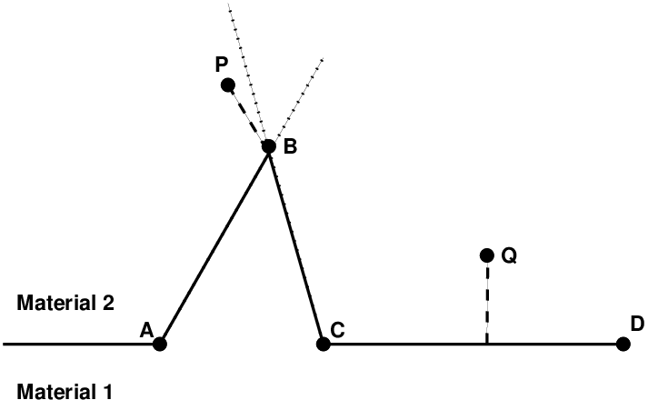
We currently use levelset functions to track the different materials in time. To initialize these levelset functions, the interfaces between the materials are defined as a number of segment vectors with the materials on the left and the right, see C for some algorithmc details. Based on these material interfaces we construct the levelset functions as smooth and signed distance from the material interface, in which the sign is positive inside the material region, while negative outside. With these levelset functions we can then reconstruct the type of material in each computational cell.
The simulations in this paper have been performed with the new 3-D laser package described in A. The numerical set-up is as follows: A laser pulse of m wavelength irradiates a m thick beryllium disk for ns. The corresponding critical electron number density, below which all light is absorbed, is cm-3. In the radiative shock experiments, the total laser energy deposition is typically kJ, but in our simulations we have to scale this down to arrive at similar results in the shock position. This laser scale factor accounts for that part of the energy for which the laser-plasma interactions cause reflection or absorption into distributions of particles that do not effectively generate ablation. These laser-plasma processes include wave-wave instabilities and related phenomena. [18] In this paper, we will use an energy of kJ. The laser spot size is m full width half maximum (FWHM) diameter. In our application, the Omega laser pulse can be represented by 10 beams with a circular cross-section and the following angles with respect to the shock tube axis: . For computational efficiency, this is modeled using 4 beams with the power per beam weighted by the number of beams approximately at that angle: one beam at , three beams at , four beams at , and two beams at . The laser profiles are spatially chosen as super-Gaussian of the order and the time profile is split in a ps linear ramp-up phase, ns with constant power, and a ps linear decay time. Each beam is discretized with 900 by 4 rays for the radial and angular coordinates of the beam cross-section. The radial beam domain size is up to 1.5 times the FWHM beam radius of m, while the angular direction is limited to half the domain due to symmetry considerations. The resulting beam resolution is sufficiently high to obtain a smooth laser heating profile, but also as coarse as possible for computational speed.
3 Radiative shocks in straight tubes
We use the CRASH code [10] to simulate both the laser energy deposition and the radiative shock propagation. This code solves the multi-material radiation-hydrodynamic equations in an operator split fashion. For each time step, we split the dynamical equations in the following way: (1) The hydrodynamic equations, level sets, and advection of radiation groups are explicitly solved with a shock capturing scheme. We typically use the HLLE scheme with a Courant–Friedrichs–Lewy (CFL) number of 0.8 and the generalized Koren limiter with . (2) Optionally we add a frequency advection in the radiation group energies caused by fluid compression. In this paper, this is switched off. (3) The contribution of the laser heating is explicitly added to the electron internal energy. In our code this energy is split between electron pressure and an extra internal energy to account for EOS corrections like the ionization, excitation, and Coulomb interactions of partially ionized ion-electron plasma. (4) The radiation diffusion, heat conduction, and energy exchanges are solved implicitly. We use a multigroup flux-limited radiation diffusion method in which the flux limiter is the square-root flux limiter [19]. For the electron thermal heat conduction, we use the so-called threshold model [14], for which the heat flux limiter has a value of . We have made several improvements to the implicit solver including the implementation of the HYPRE preconditioner, as described in B, to make the solutions more accurate. The results demonstrated below have been produced with these new code changes.
The photon energy range in our multigroup radiation model is eV – keV, which is divided in 30 groups. These groups are non-logarithmically distributed to improve the accuracy for absorption edges in the used materials. In our code, the frequency-dependent absorption coefficients are calculated internally and include the effects of Bremsstrahlung, photo-ionization of the outermost electrons, and bound-bound transitions with spectral line broadening. Multigroup opacities are then determined by averaging the absorption coefficients over the photon energy groups. The resulting specific Rosseland and Planck mean opacities for all groups are stored in lookup tables. For xenon opacities, the available atomic data provides a description of the actual structure that is too incomplete that the methods used by our code produce substantially inaccurate opacities. We therefore use for xenon high quality opacity tables calculated with the super-transition-arrays (STA) model [15] of Artep, Inc. In the relevant ranges of xenon densities and temperatures, STA produces higher opacity values than we find by running the CRASH opacity model using the limited available atomic data, e.g. for xenon at a temperature of eV and a density g/cm3 the STA opacities around eV photon energies are three orders of magnitude larger. The STA Fe and Ni opacities have recently been compared with other models in Ref. [20].
The shock tube is defined on a 2-D axial symmetric computational domain. The size of the domain is along the tube and the radius is limited to , with all distances measured in microns. The base level grid is decomposed of grid blocks of mesh cells for the and directions, respectively. Two levels of adaptive mesh refinement are applied, so that the effective grid resolution is grid cells of approximately m by m. The grid refinement is applied at all interfaces involving xenon or gold. We also apply grid refinement when the xenon mass density exceeds g/cm3 in order to resolve the xenon shock front, the electron-ion equilibration zone, and the radiative cooling layer in the shocked xenon. In addition, all beryllium to the right of m is mesh refined during the laser heating. All mentioned grid refinements are applied when any of the mentioned criteria is met in the mesh as well as ghost cells. Note that the effective cell size of m means that there are 25 cells in the -direction to span the beryllium disk thickness. This turns out to be sufficient to accurately describe the beryllium ablation and shock breakout.
The boundary conditions at the symmetry axis are reflective, while we use at all other boundaries extrapolation with zero gradient. However, for the radiation groups, we use a zero incoming flux boundary condition at the outer boundaries, i.e. all radiation leaving the computational domain will not return back.
The simulated laser energy deposition and radiative shock evolution is modeled from to ns. During the first ps the time step is reduced from about s at the very beginning of the simulation and gradually increases towards the end of the ps to a time step based on a CFL of 0.8. The increase (or decrease) in time step is controlled by the change in the extra internal energy that accounts for the ionization, excitation, and Coulomb interactions. From ps to ns, the time step is set by the default CFL number. This computation was performed on 100 processors of the FLUX supercomputer at the University of Michigan using dual socket six-core Intel Core I7 CPU nodes connected with infiniband and took hours. This includes hours and minutes for the laser heating, hours for the Krylov solver, and hours for the setup time of the HYPRE BoomerAMG preconditioner.


In Fig. 2 we show the early time response to the laser heating. The top row is for the density, electron temperature and total plasma pressure at time ns. Here one can see the early ablation of the beryllium disk, initially located between and m. The bottom row shows the same but at time ns. The region to the left of the beryllium disk is the laser corona. The region can be split in three main regions [21]: (1) The leftmost low density region is the so-called expansion region in which the plasma expands, but hardly absorbs the laser light. (2) Between the expansion region and the critical density is the absorption region where the laser energy deposition takes place. (3) Between the critical density and the not yet ablated beryllium disk is the transport region in which electron heat conduction transports heat from the low density and hot laser corona to the high density and low temperature beryllium target. It is in this region that the classical Spitzer-Härm (SH) formalism for heat transport overestimates the heat flux for the steep temperature gradients. The artificial heat flux limiter is used to prevent the SH heat conduction from exceeding the the free-streaming heat flux (see also [21]).
The resulting ablation pressure of approximately GPa drives a shock through the beryllium disk. At ps the shock has reached the right boundary of the beryllium disk. This is the shock breakout time. After this time the high pressure due to the laser heating will further accelerate the shocked plasma. In a forthcoming paper, we will present a more detailed analysis and compare the simulated shock breakout with experiments.


The shock structure at ns is shown in Fig. 3. In the top left panel the materials are displayed: xenon (black), beryllium (blue), gold (yellow), acrylic (red), polyimide (green). The two levels of dynamic mesh refinement are indicated by the black lines. The beryllium moves through the polyimide tube and drives like a piston a shock into the xenon. The compressed xenon between this shock front and the beryllium is found around m in the mass density plot of the top right panel. The plot also shows, via a black line, where the material interfaces are. The physics described in the remaining panels is similar to that in previous studies, see Ref. [11]. We repeat here only the main results for completeness. The shock velocity at ns has gradually reduced from the early velocity of km/s to about km/s. The bottom right panel shows the pressure jump at the shock, while the bottom left panel shows that the ions are shock heated. In the compressed xenon region this leads first to an electron-ion temperature equilibration due to Coulomb collisions, resulting in a cooling of the ions and heating of the electrons. Further to the left in the compressed xenon region, the electrons cool down by emitting photons. This is called the radiative cooling layer [4]. The emitted photons can propagate ahead of the shock and produce a radiative precursor as depicted in the radiation temperature panel. The sideways propagation of the radiation heats the polyimide tube. The ablation pressure of the polyimide at m in the pressure plot then drives a wall shock radially inward as is visible at the same location in the density and radial velocity plots.
The main goal of the present paper is to demonstrate that with the new improved physics fidelity and numerical schemes since the CRASH code release of Ref. [10], the radiative shock simulations in straight tubes are no longer susceptible to distortion of the dense xenon layer on axis. Indeed, the primary shock front Fig. 3 is nearly straight and only slightly slanted, but does not display the unwanted protrusion of the shock as shown in [14]. The code change that is instrumental in the improved radiative shock front is the new laser package instead of using the H2D code for the initial 1.1ns.


From the radiative shock tube experiments we obtain backlit-pinhole radiograph images [7]. These images are produced by transmitting keV through the CRASH target and in essence show regions of dense xenon. From these image we can then deduce the location of the primary and wall shock. With our code we can produce simulated X-ray radiographs, see the left panel of Fig. 4, and use such images in future code validation and uncertainty quantification. The importance of the code improvements, reported in the present paper, is that there is no longer dense xenon in front of the center of the primary shock at m and hence there is no longer a dark feature ahead of the dense xenon layer in the radiograph as in the experimentally obtained radiograph in the right panel of Fig. 4.
To demonstrate that the shock is also correct at later times, the density and radial velocity at time ns is shown in Fig. 5. The primary shock has reached m and is somewhat more slanted. The radially inward moving wall shock is at the far right in these panels.

4 Conclusions
In this paper we discussed laser-driven radiative shocks in xenon-filled straight plastic tubes. The simulations capture the shock properties seen in the laser-driven experiments and radiation-hydrodynamic theories. The laser heating ablates the beryllium target, which subsequently drives a shock through a xenon-filled tube. For laser energies of kJ, scaled down to kJ, beryllium disk thickness of m and initial xenon gas pressure of atm we obtain initial shock velocities of km/s. These shocks are fast enough to produce a radiative cooling layer in the shocked xenon. The photons can propagate ahead of the primary shock and produce a radiatively heated precursor in the unshocked xenon. The radiation also expands sideways and heats the plastic wall ahead of the primary shock. This produces an inward moving wall shock.
The numerical modeling was performed with the CRASH simulation code that solves the radiation-hydrodynamic equations on a block adaptive Eulerian grid. The hydrodynamic equations are solved explicitly, while the radiation diffusion, electron heat conduction and energy exchanges are treated implicitly. This code also includes equation-of-state and opacity solvers to enable multi-material simulations. Several code improvements have been implemented that enabled the improved quality of straight shock tube simulations. A new laser package with 3-D ray tracing has been added to CRASH so that the simulations can be performed self-consistently in one single model instead initializing the simulation runs with an external lagrangian code to evaluate the laser-energy deposition. We also incorporated highly accurate xenon opacities calculated with the super-transition-arrays (STA) model. Finally, we improved the robustness of the implicit radiation solvers with the HYPRE preconditioner instead of the original Block Incomplete Lower-Upper decomposition preconditioner. These developments greatly improved the fidelity of the radiative shock tube results.
From both the experimental and simulated X-ray radiographs, we can deduce quantities like primary shock position, wall shock position, and compressed xenon layer thickness. In future work, we will employ these type of metrics for code validation. The goal of our project is to use the validated CRASH code to perform predictive studies of three-dimemsional radiation-hydrodynamic flows, such as radiative shocks in elliptical nozzles.
Acknowledgments
This work was funded by the Predictive Sciences Academic Alliances Program in DOE/NNSA-ASC via grant DEFC52-08NA28616 and by the University of Michigan.
Appendix A Laser energy deposition library
In this appendix, we present a new package that models the laser energy transport and deposition. In previous reported radiative shock tube modeling efforts [10, 11], we used the Lagrangian radiation-hydrodynamics code H2D [12] for the first ns. This initializing of the CRASH simulations with H2D turned out to be problematic in that this produced significantly different shock structures when compared to the observations [14]. We therefore opted to implement our own laser package directly into the CRASH code. This also allows us now to simulate the radiative shock experiment in a single self-consistent model. In addition, the new laser package is parallel, while H2D is a serial code, resulting in improved computational speed.
This laser package model decomposes the laser pulse into many rays. We use a ray-tracing algorithm based on a geometric optics approximation with laser absorption via inverse Bremsstrahlung along the trajectory of the rays. Geometric optics is acceptable as long as the electron density does not vary significantly over one wavelength of the laser pulse. This is satisfied most of the time for our applications of interest, with the exception of the startup phase of the laser heating. The inverse Bremsstrahlung absorption is the most important absorption mechanism for the CRASH laser applications [21].
The laser package works both in the 2-D axi-symmetric geometry as well as in 3-D cartesian. For the axi-symmetric geometry we have implemented two versions of the the ray tracing: (1) rays confined to the axi-symmetric plane and (2) ray tracing in 3-D. In the 2-D ray tracing case we experienced the problem that all rays that are not parallel to the cylindrical axis will eventually also heat the plasma near the cylindrical axis, resulting in an excessive increase of the electron temperature near the axis. Using 3-D ray tracing in the axi-symmetric geometry mitigates this problem, resulting in improved simulations of shock break-out time and evolution of the radiative shocks compared to the 2-D rays.
Our computationally parallel ray-tracing algorithm is based on previous work on tracing radio rays in the solar corona [22]. Here, we briefly summarize the implementation as needed for the laser heating. At each time step and for each ray we trace the trajectory with a ray equation that can be derived from Fermat’s principle: a ray connecting two points and will follow a path which minimizes the integral of refractive index , i.e. the variation of the integral
| (1) |
where the independent variable is the arc-length of the ray. This can be shown, see Ref. [22], to be equivalent to
| (2) |
By introducing the ray direction, , the system (2) of three second-order differential equations is transformed in a set of six first-order equations
| (3) | |||||
| (4) |
For isotropic collisionless plasmas the refractive index is
| (5) |
where is the dielectric permittivity of the plasma, is the frequency of the laser light, and the plasma frequency depends on the electron density , electron mass , electron charge and the permittivity of vacuum . The refraction index is therefore determined from the mass density via , in which is the ion charge and the critical mass density is defined as
| (6) |
and where is the mean atomic weight and is the proton mass. This provides us with a final expression for the relative gradient of the refractive index
| (7) |
Once this gradient is known, the integration of Eqs. (3)–(4) is performed with CYLRAD algorithm [23]. The ray trace algorithm of [22] is implemented with adaptive step size to handle the steep gradients in the plasma density. For each integration step, every ray is checked for accuracy and correctness, and we ensure that rays do not penetrate in regions where .
Electron-ion collisions modify the refractive index to a complex value, where the imaginary part corresponds to absorption
| (8) |
The effective electron-ion collision frequency is defined as [24]
| (9) |
Here is the ion number density, is the Boltzmann constant, is the electron temperature, and is the Coulomb logarithm. It is due to these electron-ion collisions that the laser energy is absorbed into the plasma. The absorption coefficient (in units of 1/m) is then found as [21]
| (10) |
While performing the integration along each ray, energy is gradually deposited in the plasma.

We have added code infrastructure in CRASH to facilitate the setup of a laser pulse using a set of rays. For the sake of brevity we will only describe the 3-D laser pulse implementation in a 2-D axi-symmetric simulation. In general a 3-D laser pule will generate a 3-D laser heating, and hence 3-D simulations are required. We have code infrastructure to perform such 3-D simulations, but this is computationally expensive. In the present paper we assume that the departure from axi-symmetry is small. The laser pulse is defined with an irradiance (in units of ) and a time profile with a given linear ramp-up time, decay time, and total pulse duration. The laser pulse is further decomposed in a number of laser beams with a circular cross-section. Each beam is defined by a slope with respect to the -axis as in Fig. 6 and an initial starting point of the beam defined by and a beam offset from the -axis. For the beams we select a spatial profile of irradiance that is super-Gaussian as a function of the beam radius : , where is the beam radius and is the super-Gaussian order usually chosen to be . We use a beam margin of , beyond which the laser energy deposition is assumed to be negligible. Each beam is discretized with the same number of rays for the radial beam direction and rays for the angular direction . Due to symmetry properties for 3-D beams in axi-symmetric geometry, we only need to consider half of the angular direction of the beam, i.e. we limit to the angular beam range . The number of radial rays should be high enough to obtain a smooth laser heating profile, but as low as possible for computational speed. This number is typically chosen such that every computational cell at the critical density surface, , is crossed by at least one ray, preferably more. If the slopes of the laser beams are not too large, the number of angular rays can be selected to be small for the sake of computational speed, while still achieving sufficient accuracy.
For the laser energy deposition, we evaluate the energy emitted by the laser at each time step. The beam energy is distributed over the number of rays. The local intensity for each ray is obtained from the super-gaussian beam profile. The laser energy transport in the CRASH code uses 3-D ray-tracing based on geometric optics. During the 3-D ray tracing, we use the and positions in the axi-symmetric plane to determine where in the solution plane the laser energy deposition via inverse bremsstrahlung occurs as well as the further evaluation of the trajectory in 3-D. For these evaluations we need to map the density and density gradient into the 3-D space. A drawing of a 3-D ray projected onto the axi-symmetric plane is shown in Fig. 6. The projected ray shows not only the reflection before approaching the critical density surface and the refraction, but also the apparant reflection at a finite distance from the -axis instead of a reflection on axis. This apparant reflection is because the 3-D ray is in general not in the axi-symmetric plane and hence has a minimum distance with respect to the -axis. It is this effect that avoids the excessive laser heating on axis as is the case for 2-D rays in which the rays are confined to the axi-symmetric plane. The deposited laser energy at the current ray location in the axi-symmetric plane is distributed to the nearest computational zone volumes with the sum of the interpolation coefficents equal to one and subsequently added as an explicit source term to the right-hand-side of the electron energy density equation. The scheme is fully conservative since the total energy that is deposited by the laser pulse equals the total laser energy that is absorbed by the plasma.
Appendix B Improved radiation solver with HYPRE
In this appendix we describe the improvements in the radiation diffusion and heat conduction solvers of CRASH which led to a more robust numerical scheme. These changes were especially needed due to introduction of the laser package and the more realistic STA xenon opacities, which made the thermal heat and radiation transport stiffer in some regions.
In the applications relevant to CRASH, the electron temperature does not change much in the energy exchange between the electrons and radiation. We can therefore first solve for the electron and ion temperature, and , without taking into account the energy exchange with the radiation. Discretizing the heat conduction and electron-ion energy exchange in time leads to the following backward Euler scheme:
| (11) | |||||
| (12) |
where and are ion and electron specific heat, is the heat conduction coefficient, and is the coupling coefficient that depends on the ion-electron relaxation time. These coefficients are frozen in at time level during the time advance from time level to . The scheme is therefore temporally first order. The time level indicates that we still have to perform an update for the electron-radiation energy exchange. The backward Euler equations for the radiation group energies can be written as
| (13) |
in which is proportional to the group mean Planck opacity, while is the group energy of the blackbody radiation. The radiation diffusion coefficient depends on the group mean Rosseland opacity. Our multigroup model is flux limited and the flux limiter is incorporated in . By introducing the change in the electron temperature and radiation group energies , Eqs. (11)–(13) can be combined into equations for these changes
| (14) | |||||
| (15) |
where we exploited that Eq. (11) is point-implicit, which results in the modified ion-electron couplings coefficient . The is the Planck weight. To obtain a discretized set of equations, we use the scheme proposed in [11]. This numerical scheme is overall spatially second-order, consistent, and conservative. Here it suffices to mention that once numerical solutions are obtained for these equations by means of a linear solver, the energy densities for the radiation groups, ions, and electrons are updated using
| (16) | |||||
| (17) | |||||
| (18) |
These updates conserve the total energy to round-off errors. We note that we changed the Eqs. (11) and (12) to solve for the temperatures and instead of the plackian quantities and as described in Ref. [10]. This improves the scheme at low temperatures, since we no longer have divisions by temperatures in this system.
The implicit scheme in CRASH uses a preconditioned Krylov solver: GMRES, BiCGSTAB, or preconditioned conjugate gradient (PCG) as described in Ref. [10]. Our original preconditioner is based on the Incomplete Lower Upper (ILU) decomposition with no fill-in. Since CRASH uses a block-adaptive grid, we find it advantageous to use a Schwartz type preconditioning on a block-by-block basis [25]. While the block ILU preconditioner gives satisfactory results for small to medium problem size, the number of Krylov iterations can easily be a few 100s to even 1000s on large problems due to the stiffness of the linear system. In addition, some of the radiation groups with small energy content fail to converge due to round-off errors.
As an alternative to the ILU preconditioner, we have implemented an interface with an algebraic multi-grid (AMG) preconditioner into CRASH. We use the BoomerAMG solver from the HYPRE library [16]. This preconditioner requires much fewer Krylov iterations than the ILU preconditioner, but the AMG iterations are much more expensive. The BoomerAMG has also a setup time at the beginning of the Krylov solve that is rather significant, and does not scale well to many processors. Despite these issues, we find in our latest 2-D simulations with the new laser package and improved opacities that using AMG results in a more accurate solutions than the ILU preconditioner. HYPRE also allows us to set more demanding tolerance criteria for the implicit solver and still obtain converged solution in a small number of iterations. For the typical laser-driven radiative shock simulations of the CRASH project it turns out that BoomerAMG of HYPRE outperforms the ILU preconditioner in computational time.
Appendix C Material interface
Figure 7 shows two different materials separated by an interface consisting of 4 straight segments. For every point in the plane, we find the closest segment. For example, for point Q the closest segment is CD. Since Q is on the left side of the CD vector (directed from point C to D), it belongs to material 2, and its level set function is set by the normal distance to segment CD, indicated by the dashed line. For point P, however, there are two closest segments: AB and BC. P lies on the left side of the AB vector, which corresponds to material 2, but on the right side of the BC vector, which would indicate material 1. In general there can be several interface segments at the same minimal distance from point P. One can show that it is always the segment that has the largest normal distance from the point, in this case segment AB, that signals the correct material.
References
- [1] P.A. Keiter, R.P. Drake, T.S. Perry, H.F. Robey, B.A. Remington, C.A. Iglesias, R.J. Wallace, J. Knauer, Observation of a hydrodynamically-driven, radiative-precursor shock, Phys. Rev. Lett. 89 (2002) 165003-1.
- [2] S. Bouquet, C. Stéhlé, M. Koenig, J.-P. Chièze, A. Benuzzi-Mounaix, D. Batani, S. Leygnac, X. Fleury, H. Merdji, C. Michaut, F. Thais, N. Grandjouan, T. Hall, E. Henry, V. Malka, J.-P.J. Lafon, Observations of laser driven supercritical radiative shock precursors, Phys. Rev. Lett. 92 (2004) 225001.
- [3] M. Koenig, T. Vinci, A. Benuzzi-Mounaix, N. Ozaki, A. Ravasio, M. Rabec le Glohaec, L. Boireau, C. Michaut, S. Bouquet, S. Atzeni, A. Schiavi, O. Peyrusse, D. Batani, Radiative shocks: An opportunity to study laboratory astrophysics, Phys. Plasmas 13 (2006) 056504.
- [4] A.B. Reighard, R.P. Drake, The formation of a cooling layer in a partially optically thick shock, Astrophys, Space Sci. 307 (2007) 121–125.
- [5] G. Gregori, A. Ravasio, C.D. Murphy, K. Schaar, A. Baird, A.R. Bell, A. Benuzzi-Mounaix, R. Bingham, C. Constantin, R.P. Drake, M. Edwards, E.T. Everson, C.D. Gregory, Y. Kuramitsu, W. Lau, J. Mithen, C. Niemann, H.-S. Park, B.A. Remington, B. Reville, A.P.L. Robinson, D.D. Ryutov, Y. Sakawa, S. Yang, N.C. Woolsey, M. Koenig, F. Miniati, Scaled protogalactic magnetic field generation in laser-produced shock waves, Nature 481 (2012) 7382.
- [6] H.-S. Park, D.D. Ryutov, J.S. Ross, N.L. Kugland, S.H. Glenzer, C. Plechaty, S.M. Pollaine, B.A. Remington, A. Spitkovsky, L. Gargate, G. Gregori, A. Bell, C. Murphy, Y. Sakawa, Y. Kuramitsu, T. Morita, H. Takabe, D.H. Froula, G. Fiksel, F. Miniati, M. Koenig, A. Ravasio, A. Pelka, E. Liang, N. Woolsey, C.C. Kuranz, R.P. Drake, M.J. Grosskopf, Studying astrophysical collisionless shocks with counterstreaming plasmas from high power lasers, High Energy Density Phys. 8 (2012) 38–45.
- [7] F.W. Doss, H.F.Robey, R.P. Drake, C.C. Kuranz, Wall shocks in high-energy-density shock tube experiments, Phys. Plasmas 16 (2009) 112705.
- [8] F.W. Doss, R.P. Drake, C.C. Kuranz, Repeatability in radiative shock tube experiments, High Energy Density Phys. 6 (2010) 157–161.
- [9] T.R. Boehly, R.S. Craxton, T.H. Hinterman, J.H. Kelly, T.J. Kessler, S.A. Letzring, R.L. McCrory, S.F.B. Morse, W. Seka, S. Skupsky, J.M. Soures, C.P. Verdon, The upgrade to the omega laser system, Rev. Sci. Instr. 66 (1995) 508.
- [10] B. van der Holst, G. Tóth, I.V. Sokolov, K.G. Powell, J.P. Holloway, E.S. Myra, Q. Stout, M.L. Adams, J.E. Morel, S. Karni, B. Fryxell, R.P. Drake, A block-adaptive-mesh code for radiative shock hydrodynamics: Implementation and verification, Astrophys. J. Suppl. 194 (2011) 23.
- [11] B. van der Holst, G. Tóth, I.V. Sokolov, L.K.S. Daldorff, K.G. Powell, R.P. Drake, Simulating radiative shocks in nozzle shock tubes, High Energy Density Phys. 8 (2012) 161.
- [12] J.T. Larsen, S.M. Lane, Hyades: a plasma hydrodynamics code for dense plasma studies, J. Quant. Spectrosc. Radiat. Transf 51 (1994) 179–186.
- [13] G. Tóth, B. van der Holst, I.V. Sokolov, D.L. De Zeeuw, T.I. Gombosi, F. Fang, W.B. Manchester, X. Meng, D. Najib, K.G. Powell, Q.F. Stout, A. Glocer, Y.-J. Ma, M. Opher, Adaptive Numerical Algorithms in Space Weather Modeling, J. Comp. Phys. 231 (2012) 870.
- [14] R.P. Drake, F.W. Doss, R.G. McClarren, M.L. Adams, N. Amato, D. Bingham, C.C. Chou, C. DiStefano, K. Fidkowsky, B. Fryxell, T.I. Gombosi, M.J. Grosskopf, J.P. Holloway, B. van der Holst, C.M. Huntington, S. Karni, C.M. Krauland, C.C. Kuranz, E. Larsen, B. van Leer, B. Mallick, D. Marion, W. Martin, J.E. Morel, E.S. Myra, V. Nair, K.G. Powell, L. Raushberger, P. Roe, E. Rutter, I.V. Sokolov, Q. Stout, B.R. Torralva, G. Tóth, K. Thornton, A.J. Visco, Radiative Effects in Radiative Shocks in Shock Tubes, High Energy Density Phys. 7 (2011) 130.
- [15] A. Bar-Shalom, J. Oreg, W.H. Goldstein, D. Shvarts, A. Zigler, Super-transition-arrays: A model for the spectral analysis of hot dense plasma, Phys. Rev. A (At. Mol. Opt. Phys.) 40 (1989) 3183–3193.
- [16] R.D. Falgout, U.M. Yang, hypre: a Library of High Performance Preconditioners, in Computational Science - ICCS 2002 Part III, P.M.A. Sloot, C.J.K. Tan. J.J. Dongarra, and A.G. Hoekstra, eds., vol. 2331 of Lecture Notes in Computer Science, Springer-Verlag (2002), pp. 632-641. UCRL-JC-146175.
- [17] J.P. Holloway, D. Bingham, C. Chou, F. Doss, R.P. Drake, B. Fryxell, M. Grosskopf, B. van der Holst, R. McClarren, A. Mukherjee, V. Nair, K.G. Powell, D. Ryu, I. Sokolov, G. Tóth, Z. Zhang, Predictive Modeling of a Radiative Shock System, Reliability Engineering and System Safety 96 (2011) 1184.
- [18] W.L. Kruer, The physics of Laser-Plasma Interactions (Westview Press, Reprint Edition, Boulder, C0, 2001).
- [19] J.E. Morel, Diffusion-limit asymptotics of the transport equation, the P1/3 equations, and two flux-limited diffusion theories, J. Quant. Spectrosc. Radiat. Transf 65 (2000) 769–778.
- [20] D. Gilles, S. Turck-Chièze, G. Loisel, L. Piau, J.-E. Ducret, M. Poirier, T. Blenski, F. Thais, C. Blancard, P. Cossé, G. Faussurier, F. Gilleron, J.C. Pain, Q. Porcherot, J.A. Guzik, D.P. Kilcrease, N.H. Magee, J. Harris, M. Busquet, F. Delahaye, C.J. Zeippen, S. Bastiani-Ceccotti, Comparison of Fe and Ni opacity calculations for a better understanding of pulsating stellar envelopes, High Energy Density Phys. 7 (2011) 312–319.
- [21] R.P. Drake, High Energy Density Physics: Fundamentals, Inertial Fusion and Experimental Astrophysics. Springer, Verlag, 2006.
- [22] L. Benkevitch, I. Sokolov, D. Oberoi, T. Zurbuchen, Algorithm for Tracing Radio Rays in Solar Corona and Chromosphere, arXiv:1006.5635v3 (2010).
- [23] J.P. Boris, Relativistic Plasma Simulation — Optimization of a Hybrid Code, in Proc. 4th Conf. Num. Sim. Plasmas, Naval Res. Lab. (1971) 3–-67.
- [24] V.L. Ginzburg, The Propagation of Electromagnetic Waves in Plasmas. (Pergamon Press, 1964).
- [25] G. Tóth, D.L. De Zeeuw, T.I. Gombosi, K.G. Powell, A parallel explicit/implicit time stepping scheme on block-adaptive grids, J. Comp. Phys. 217 (2006) 722–-758.