A Coverage Theory of Bistatic Radar Networks:
Worst-Case Intrusion Path and Optimal Deployment
Abstract
Continuing advances in radar technology are driven both by new application regimes and technological innovations. A family of applications of increasing importance is detection of a mobile target intruding into a protected area, and one type of radar system architecture potentially well suited to this type of application entails a network of cooperating radars. In this paper, we study optimal radar deployment for intrusion detection, with focus on network coverage. In contrast to the disk-based sensing model in a traditional sensor network, the detection range of a bistatic radar depends on the locations of both the radar transmitter and radar receiver, and is characterized by Cassini ovals. Furthermore, in a network with multiple radar transmitters and receivers, since any pair of transmitter and receiver can potentially form a bistatic radar, the detection ranges of different bistatic radars are coupled and the corresponding network coverage is intimately related to the locations of all transmitters and receivers, making the optimal deployment design highly non-trivial. Clearly, the detectability of an intruder depends on the highest SNR received by all possible bistatic radars. We focus on the worst-case intrusion detectability, i.e., the minimum possible detectability along all possible intrusion paths. Although it is plausible to deploy radars on a shortest line segment across the field, it is not always optimal in general, which we illustrate via counter-examples. We then present a sufficient condition on the field geometry for the optimality of shortest line deployment to hold. Further, we quantify the local structure of detectability corresponding to a given deployment order and spacings of radar transmitters and receivers, building on which we characterize the optimal deployment to maximize the worst-case intrusion detectability. Our results show that the optimal deployment locations exhibit a balanced structure. We also develop a polynomial-time approximation algorithm for characterizing the worse-case intrusion path for any given locations of radars under random deployment.
keywords
bistatic radar networks, network coverage, optimal deployment, worst-case intrusion path1 Introduction
1.1 Motivation

An active radar system consists of a collection of transmitters and receivers in which transmitters emit RF signals and the receivers capture signals resulting from scattering of the transmitted signals reflected by objects of interest (targets). A monostatic radar is one in which a single transmitter and single receiver are collocated. A bistatic radar is also comprised of a single transmit-receive pair, but the transmitter and receiver are at different locations. Multistatic radar refers to a configuration that consists of multiple receivers at different locations. Although physical-layer issues in radar have been extensively studied [1], very limited attention has been paid to radar network design [2, 3, 4]. Notably, [2] considered a network of monostatic radars, and [3, 4] studied a multistatic radar with one transmitter. We are thus motivated to consider a network of multiple radar transmitters and receivers where any pair of transmitter and receiver can form a bistatic radar. Unlike traditional passive sensors, one salient feature of radar sensing is that it actively emits signals to illuminate the target. Further, radar technology provides superior penetration capability by using radio waves. Worth mentioning is that the cost of radars can be much higher than traditional sensors.
The problem of detecting intrusion into a protected area, across a border or security perimeter, is of increasing interest for numerous applications, and has great potential in several regimes of growing importance, such as border monitoring, industrial and airport security, and drug interdiction. Worst-case coverage [5] is a common criterion of efficacy in intrusion detection that has been applied extensively in the context of sensor networks [6, 7, 8, 9]. It is intimately related to the minimum possible detectability of an intruder (target) traversing a monitored field. In a bistatic radar network, the worst-case coverage is quite different and more difficult to quantify than traditional sensor networks, because 1) departing from the disk-based sensing range of a traditional sensor, the detection range of a bistatic radar depends on the locations of both radar transmitter and receiver and is characterized by the Cassini oval (in scenarios where intruder detectability is dominated by SNR). Formally, a Cassini oval is a locus of points for which the distances to two fixed points (foci) have a constant product (as illustrated in Figure 1); 2) the sensing ranges of different bistatic radars are coupled with each other, since each transmitter (or receiver) can pair with other receivers (or transmitters) to form multiple bistatic radars, indicating that its location would impact multiple bistatic radars.
1.2 Summary of Main Contributions
- •
We first rigorously quantify the intrusion detectability and network coverage attainable by a bistatic radar network, while taking into account the complication that each pair of transmitter and receiver can potentially form a bistatic radar. We then study the worst-case coverage under deterministic deployment, aiming to find optimal deployment locations of radar transmitters and receivers such that the worst-case intrusion detectability is maximized. We present a sufficient condition on the field geometry under which it is optimal to deploy radars on a shortest line segment across the field, which we refer as a shortcut barrier. The line barrier appears intuitive but does not hold for arbitrary field geometry, for which we give counter-examples. Further, when radars are deployed on the shortcut barrier, the worst-case intrusion detectability turns out to be the vulnerability of the shortcut barrier, which is the minimum detectability of all points on it.
- •
A main thrust of this study is devoted to characterizing the optimal deployment locations of radars on the shortcut barrier to minimize its vulnerability. Since the optimization problem is neither differentiable nor convex, it is highly non-trivial to solve. We first quantify the local structure of detectability corresponding to a given deployment order and spacings along a shortcut barrier. Then, for a given deployment order, we establish the existence and optimality of balanced deployment spacings required to attain the minimum vulnerability. Next, we derive sufficient conditions for an optimal deployment order, and characterize the corresponding optimal deployment orders. Our findings reveal that the optimal deployment locations exhibit a balanced structure. Furthermore, under the optimal deployment, it suffices for a receiver to form at most two bistatic radars to guarantee the optimal coverage quality, under the condition that the number of receivers is no less than that of transmitters (which is often the case since radar transmitters are more costly).
- •
We also study the worst-case coverage under random deployment, and quantify the worst-case intrusion path for any given deployment of radars. In particular, by developing a novel 2-site Voronoi diagram with graph search techniques, we design an algorithm to find an approximate worst-case intrusion detectability, where the approximation error can be made arbitrarily small. The algorithm is shown to have polynomial-time complexity.
We believe that the studies we initiated here on bistatic radar networks scratch only the tip of the iceberg. There are still many questions remaining open for the design of a networked radar system.
The rest of this paper is organized as follows. Section 2 introduces the model of worst-case coverage for the bistatic radar network. In Section 3, we characterize the optimal deployment of radars for maximizing the worst-case detectability. Section 4 presents an efficient algorithm for finding an approximate worst-case detectability given arbitrary locations of radars. Section 5 provides the evaluation results. Related works are discussed in Section 6. The paper is concluded in Section 7.
2 System Model
Basic Setting. We consider a bistatic radar network deployed in a field of interest . The field is a bounded and connected region enclosed by four curves: a left boundary , a right boundary , an entrance side, and a destination side (see Figure 2). Note that we allow the boundary curves of the field to be arbitrary. An intruder (target) can traverse through along any intrusion path from a point on the entrance to a point on the destination. Specifically, the bistatic radar network consists of radar transmitters , and radar receivers , . We assume that each pair of transmitter and receiver can potentially form a bistatic radar. We further assume that orthogonal transmissions are used for interference avoidance. For convenience, we also use or to denote the location (point) of node or , respectively.
Bistatic radar SNR and Cassini Oval. For a bistatic radar, the received SNR for a target is given by
| (1) |
where and denote the transmitter-target and receiver-target distances, respectively, and denote bistatic radar constant which reflects physical-layer system characteristics, such as transmitting power, radar cross section, and transmitter/receiver antenna power gains. For ease of exposition, we assume the bistatic radar constant is the same, and our study on homogeneous bistatic radars here will serve as a major step for studying the heterogenous case. Given a bistatic radar, the SNR contours are characterized by the Cassini ovals with foci at the transmitter and receiver. We use to denote the Cassini oval with foci at points and for constant distance product .
Intrusion Detectability and Network Coverage. Let denote the (Euclidean) distance between two points and . It follows from (1) that the received SNR by a bistatic radar from a target at some point is determined by the distance product . Then the detectability of a point is quantified by the minimum distance product from to all bistatic radars, denoted by
| (2) |
Observe from (2) that the detectability increases when reduces, and vice versa. The detectability of an intruder is captured by the detectability of its intrusion path , which is the maximum detectability of all points on , denoted by
| (3) |
From the radar network’s perspective, in the worst case, the intruder traverses through along an intrusion path such that is maximized. We refer this path and its detectability as the worst-case intrusion path and the worst-case intrusion detectability (WID), respectively.
3 Deterministic Deployment
We consider both deterministic deployment and random deployment scenarios, in the same spirit as the arbitrary/random network models in the seminal work by Gupta and Kumar [10]. In the deterministic deployment case, our goal is to find optimal deployment locations of radar nodes (i.e., transmitters and receivers) in such that WID is maximized, i.e.,
| (4) |
The above problem is highly non-trivial in general since the boundaries of field can be arbitrary. In particular, we are interested in the line-based deployment scheme in which radars are deployed along a line which is simple to implement in practice. Further, we will show that it is optimal under some mild condition on the field geometry. To the best of our knowledge, the optimality of line-based deployment for worst-case coverage has not been studied in literature.
3.1 Shortcut Barrier-based Deployment
We need the notion of barrier to establish our results on the line-based deployment. Given any , the detection range of a bistatic radar , denoted by , is the region enclosed by the Cassini oval such that for all . The detection range of the bistatic radar network, denoted by , is the union of the detection ranges of all the bistatic radars. A barrier is a curve in the field connecting the left boundary and right boundary such that any intrusion path through intersects with the barrier. The worst-case coverage is intimately related to the notion of barrier as given in the next property. The proof is based on an argument similar to the growing disks in [7] and is omitted here.
Property 1
The worst-case intrusion detectability is equal to the smallest value of such that there exists a barrier in the network’s detection range .
We define the vulnerability of a barrier as the minimum detectability of all points in , denoted by
| (5) |

Intuitively, we expect to attain the best coverage quality by deploying radars along a shortest barrier which an intruder must pass through. We make the following assumption on the geometry of field .
Assumption 1
There exists a shortest line segment connecting and such that .
Although a shortest line segment connecting and always exists, it is critical to assume that it lies in the field (see Figure 2). We refer such an as the shortcut barrier (SCB) and let denote its length. In other words, is the shortest distance between a point in and a point in . Note that a shortcut barrier is always a shortest barrier that has the shortest length among all barriers, but the converse is not true (as illustrated in Figure 2). Assumption 1 captures a large class of field geometry, e.g., any of convex shape belongs to this class.
The next result shows that the SCB-based deployment is indeed optimal if the shortcut barrier exists. (All proofs of the theorems and lemmas in the sequel are relegated to Appendix).
Theorem 1
Under Assumption 1, it is optimal to deploy radars on the shortcut barrier , in order to maximize the worse-case intrusion detectability.
Although Theorem 1 appears intuitive, we caution that it is non-trivial since the proof hinges on the existence of a shortcut barrier such that a line barrier with no greater vulnerability can be constructed from any arbitrary barrier. In other words, if the shortcut barrier does not exist, the optimal deployment may not be on a shortest barrier (see Figure 2(b)).
Let and denote the end points of with and . Note that the worst-case intrusion detectability under a line-based deployment is no greater than, but not necessarily equal to, the vulnerability of the line segment. However, the equality holds for the SCB-based deployment as we show in the next result.
Theorem 2
Under Assumption 1, if radars are deployed on the shortcut barrier , the worst-case intrusion detectability amounts to the vulnerability of , i.e., .
3.2 Line-based Optimal Deployment Locations
In this subsection, we study the optimal deployment locations of radars on the shortcut barrier to minimize . Let and . Mathematically, our problem can be formulated as
| (6) | ||||
where represents the detectability of a point with . It can be easily checked that the objective function of problem (6) is neither differentiable nor convex in general. Therefore, standard optimization methods can not be applied here.
Consider the reformulation of problem (6) as follows. First, we treat and as two virtual nodes and relax the constraint . Suppose all nodes in and as well as and are deployed on a line such that and are the leftmost and rightmost nodes, respectively. Let denote a deployment order (“order” for short) of all nodes, where and is a permutation of the set such that . Without ambiguity, also denote an order of locations of all nodes. Let denote the deployment spacings (“spacings” for short) of a given deployment order of nodes , which are the distances between all pairs of neighbor nodes in . Similarly, let denote a deployment suborder (“suborder” for short), which is a deployment order of neighbor nodes in , and denote its deployment spacings. Clearly, any deployment order with any deployment spacings represent some deployment locations of and on a line segment with length . Likewise, any deployment locations of and on the line barrier can be represented by some deployment order with some deployment spacings under the constraint . To summarize, the problem (6) can be recast as
Problem 1
Find an optimal deployment order with optimal deployment spacings under the constraint such that is minimized.
In what follows, we outline the main steps to solve Problem 1.
- Step1:
We show a general and important structure of detectability on (Lemma 1), which leads to the concept of balanced spacings.
- Step2:
- Step3:
We rule out some orders from consideration, which leads to the concept of candidate order (Lemma 4). Then we show that a candidate order consists of decoupled local suborders, such that the results in Step 2 can be applied to show that balanced spacings exist and are optimal for a candidate order (Theorem 3).
- Step4:
Based on the optimal spacings obtained above, we derive sufficient conditions for an optimal order (Theorem 4). Then we characterize the optimal orders.
We start with two observations. First, swapping the locations of any pair of transmitters or any pair of receivers results in an equivalent deployment. Second, transmitters and receivers are reciprocal to each other. Specifically, replacing all transmitters by receivers and replacing all receivers by transmitters results in an equivalent deployment. These observations will be used repeatedly in the sequel.
Let denote the midpoint between two points and . In the next lemma, we show a local structure for the vulnerability of .
Lemma 1
Given any order with any spacings , attains local maximums on at the end nodes and , and at the midpoints of all pairs of neighbor nodes in (as depicted in Figure 3). In particular,

For convenience, we refer a local maximum point of and its value as a local vulnerable point and local vulnerable value, respectively. The local structure presented in Lemma 1 is essentially due to that the detectability of a point is dominated by the closet transmitter and receiver. Therefore, it suffices to characterize the local vulnerable values at the local vulnerable points to determine the vulnerability of . We say the spacings of an order of nodes are balanced if all the local vulnerable values between or on the two end nodes of that order are equal (see Figure 3).
We define the pattern of an order of nodes as the order of node types (transmitter type or receiver type ) of those nodes. We use or to denote consecutive or in a pattern, respectively. We define three kinds of local patterns , , , or for , or for , and or . We say a suborder is a local suborder if it has a local pattern, and it is associated with a local zone, denoted by , which is the line segment between the two end nodes of that local suborder. For example, if , then . The vulnerability of a local zone is . We denote the length of by .
We observe that for any local suborder with any spacings, the closest transmitter and receiver from for any local vulnerable point in are nodes from . For example, if , we can see that the closest transmitter and receiver for are and , respectively; if , the closest transmitter for any of , , , , is , and the closest receiver for any of , , , , is from . Hence, the vulnerability of a local zone , i.e., , only depends on the locations of nodes in , or in other words, depends on the spacings , and it is independent of the locations of nodes not in . Similar observations can be made for any local suborder. Using Lemma (1), in the next result, we characterize the balanced spacings of a local suborder.
Lemma 2
For any , let and be the unique positive value of such that
for any . Given any and any local suborder , there
exist unique spacings such that is balanced with . Furthermore, it is given by, e.g., if , then ;
if
, , then
if and is even, then
or if is odd, then
where the arguments “” of are omitted for brevity. Similar results can be obtained for any other local suborder.
By definition, given , the value of , can be found iteratively and it decreases as increases (see Table 1).
| c | |||||
|---|---|---|---|---|---|
| 1 | 2.0000 | 0.8284 | 0.6357 | 0.5359 | 0.4721 |
| 5 | 4.4721 | 1.8524 | 1.4214 | 1.1983 | 1.0557 |
| 10 | 6.3246 | 2.6197 | 2.0102 | 1.6947 | 1.4930 |
| 20 | 8.9443 | 3.7048 | 2.8428 | 2.3966 | 2.1115 |
The following lemma shows that balanced spacings are optimal for a local suborder.
Lemma 3
Given any local suborder , suppose is balanced with . If is the same local suborder as and with spacings such that , then . Furthermore, if , then .
Lemma 3 suggests that given a local suborder and a constraint on the local zone’s vulnerability, the balanced spacings maximize the length of the local zone.
We need the following lemma which reduces our search space significantly.
Lemma 4
There exists an optimal order not having a suborder with any of the following patterns: , , , , , , , and .
We say an order is a candidate order if it does not have a suborder with any of the patterns given in Lemma 4.
We observe that any given candidate order consists of a series of local suborders such that 1) each node in is included in some ; 2) the last node of is the first node of for all . In particular, and have patterns , and has pattern or for . For example,
Accordingly, consists of a series of local zones , , , and consists of a series of spacings , , . To see why such a series of local suborders exists for any given candidate order , we construct a super order from by combining neighbor nodes of the same type in into a super node. A node not combined in is a simple node in . For the above example, the super order is given by
It is clear by our construction that two neighbor nodes in (excluding and ) are of different types (transmitter type or receiver type). Since is a candidate order, it does not have a suborder with any pattern given in Lemma 4. Hence, it can be easily checked that two neighbor nodes in can not be both super nodes, and a super node can not be the third or third-to-last node in . Then we can see that the first three nodes and the last three nodes in represent two local suborders with patterns ; each super node and its two neighbor simple nodes in represent a local suborder with pattern ; two neighbor simple nodes not at the beginning or end of (excluding and ) represent a local suborder with pattern .
The decoupled structure of a candidate order allows us to apply results of local suborders. Consider a given candidate order . We know that consists of a series of local suborders . As a result, the set of local vulnerability values on is a union of disjoint sets of local vulnerability values on all the local zones , , . Therefore, since local vulnerability values on a local zone only depend on the corresponding spacings , we can see that is balanced with if and only if is balanced with for all . Hence, by Lemma 2, there exists unique such that is balanced with .
We observe that given a candidate order , under the constraint that is balanced with , varies as a function of . It follows from Lemma 2 that each of , , is an increasing function of , and hence is also an increasing function of . Furthermore, it can be easily verified that when and when . Thus, there exists a unique such that . This implies that under the constraint , there exist unique balanced . We summary this result below as a corollary of Lemma 2.
Corollary 1
Given any candidate order , under the constraint , there exist unique spacings such that is balanced.
Applying Lemma 3, we obtain the following theorem.
Theorem 3
Given any candidate order , the unique balanced spacings minimize under the constraint .
Theorem 3 suggests that the optimal spacings for any given candidate order is the unique balanced spacings referred in Corollary 1.
Since we have found the optimal spacings for any candidate order , our next step is to find an optimal order . Suppose the number of transmitters is no greater than the number of receivers, i.e., , WLOG. Since all transmitters are equivalent, we suppose that transmitters in are indexed by their order in such that . Define where , , and denote the number of receivers between and , between and , and between and , respectively, in . Since all receivers are equivalent, it suffices to determine , , and for an optimal order. The next result provides sufficient conditions for the optimality of an order.
Theorem 4
A candidate order is optimal if
Using the optimality conditions in Theorem 4, we can find an optimal order described as follows. Let two integers and be the quotient and remainder of . If is even, there exists an such that
if is odd and , there exists an such that
if is odd and , there exists an such that
It can be easily seen that any order obtained from the above optimal order by exchanging the values of and , or the values of and for some , also satisfies the optimality condition, and hence is optimal. We observe that the optimal order also exhibits a balanced structure.
Given an optimal order , by Theorem 3, the optimal spacings is the unique balanced spacings under the constraint . The optimal spacings can be found by a bisection search. In each search step, for a search criterion , we can obtain by Lemma 2 the unique balanced spacings with , and hence obtain . If , is decreased for the next step; if , is increased for the next step. The search completes if . Upon completion, the optimal spacings is found and the optimal value of is equal to the search criterion .
4 Random Deployment
Next, we consider random deployment that can also be of great interest. In this scenario, given arbitrary locations of radars resulted from random deployment, we aim to find the worst-case intrusion path and the worst-case intrusion detectability . Due to the complex geometry of bistatic radar SNR, it is difficult to find accurately. Therefore, we design an efficient algorithm for finding an intrusion path whose detectability is arbitrarily close to . Our algorithm partitions the field into sub-regions based on a novel 2-site Voronoi diagram, and then constructs a weighted graph for the sub-regions to search for an approximate worst-case intrusion path .
Given a set of points , the Voronoi region of a point is the set of points which are closer to than to any other point in , i.e.,
| (7) |
The Voronoi diagram for is the collection of all Voronoi regions . To partition the field , we first construct Voronoi diagrams for the set of transmitters and the set of receivers , respectively, i.e., and , within the boundaries of . Then can be partitioned into 2-site Voronoi regions, where a 2-site Voronoi region, denoted by , is the intersection of a transmitter Voronoi region and a receiver Voronoi region, i.e.,
| (8) |
for all and such that (see Figure 5). Choose an arbitrary . For each 2-site Voronoi region , we plot a sequence of Cassini ovals for consecutive positive integer values of such that is further divided by these Cassini ovals into sub-regions where each sub-region is bounded between two Cassini ovals with distance products being consecutive multiples of .
We construct a graph where each vertex represents a sub-region, and two vertices are connected by an edge if they are adjacent sub-regions. Then we assign each vertex a weight , which is equal to the smaller distance product of the two Cassini ovals bounding this sub-region. We add two virtual vertices and to represent the entrance and destination of , respectively. There exists an edge between vertex and for if sub-region is adjacent to the entrance. Similarly, we add an edge between vertex and for if sub-region is adjacent to the destination.
It is clear that any intrusion path is represented by an path in , denoted by . We define the weight of an path , denoted by , as . We aim to find an path with maximum weight. This can be obtained by a bisection search between the smallest and largest vertex weights in . In each step, breadth-first-search is used to check the existence of a path using only vertices with weights larger than a search criterion . If a path exists, is increased to restrict the vertices considered in the next search step; otherwise, is decreased to relax the constraint on the search. Upon completion, a path with maximum weight is found.

Suppose and . The number of vertices in graph , i.e., the number of sub-regions in field , is and the reason is as follows. We can treat the field as a planar graph, where the vertices are the crossing points of Voronoi edges and Cassini ovals, and the edges are line segments or curves between two crossing points. The number of Voronoi edges and the number of Voronoi vertices are both . So the number of crossing points of Voronoi edges is . Hence, the number of 2-site Voronoi vertices is , and the number of 2-site Voronoi edges is . Since the field is bounded, the number of Cassini ovals plotted for a 2-site Voronoi region is . So the total number of crossing points of Cassini ovals with 2-site Voronoi edges is . Hence, the number of vertices of sub-regions is , and the number of edges of sub-regions is . By Euler’s formula, the number of faces, which is the number of sub-regions, is 2 - + , equal to .
In the next result, part (a) follows from the definition of 2-site Voronoi diagram and our graph construction; part (b) follows from our result on the number of vertices in graph . The proof is omitted due to space limitation.
Theorem 5
(a) The maximum path weight obtained by our proposed approximation algorithm is within to the worst-case detectability, i.e.,
| (9) |
(b) Given , our proposed approximation algorithm has polynomial-time complexity.
5 Performance Evaluation
In this section, we present some numerical results to illustrate the effectiveness of our proposed optimal radar deployment scheme.
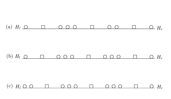
We examine the vulnerability of a line segment under the line-based deployment. In particular, we compare the optimal deployment scheme (OPT) with two heuristic deployment schemes. The first heuristic (HEU-1) is to deploy radar transmitters (or receivers, respectively) with uniform spacings such that the maximum distance from a point on to its closet transmitter (or receiver, respectively) is minimized (see Figure 6). Specifically, HEU-1 results in and , where transmitters and receivers are indexed by their orders in , respectively. It can be easily verified that this scheme is optimal if we treat radar transmitters (or receivers, respectively) as traditional sensors with disk-based sensing model. The second heuristic (HEU-2) is to deploy radar transmitters and receivers according to an optimal order from OPT but with uniform spacings such that the maximum distance from a point on to its closet transmitter or receiver is minimized (see Figure 6). Specifically, HEU-2 results in .

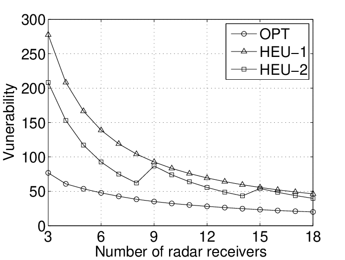
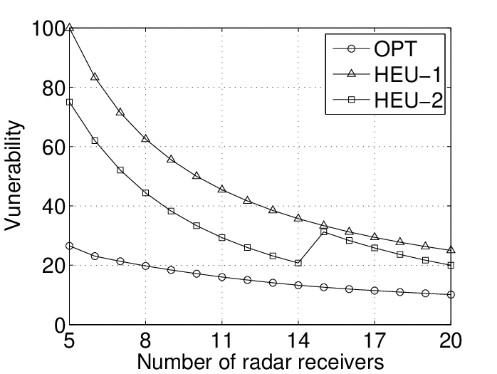
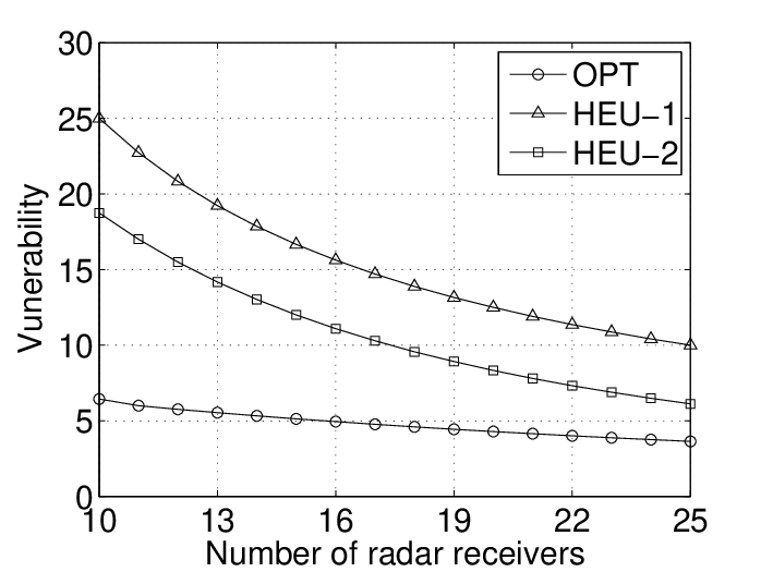
Figure 7, Figure 8 and Figure 9 depict the vulnerability of versus the number of radar receivers for , , and radar transmitters, respectively, where we set . We note that HEU-2 results in considerably lower vulnerability than HEU-1. This is because HEU-1 deploys transmitters and receivers independently, while HEU-2 takes into account the joint design of transmitters and receivers. We observe that OPT further outperforms HEU-2 significantly. This suggests that optimal spacings is critical for improving the performance due to the complex geometry of bistatic radar SNR.
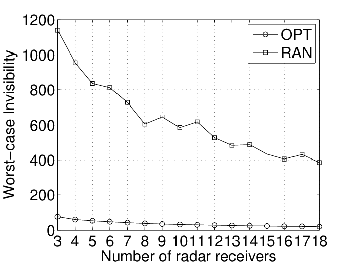
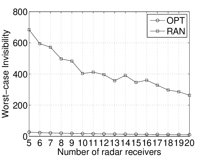
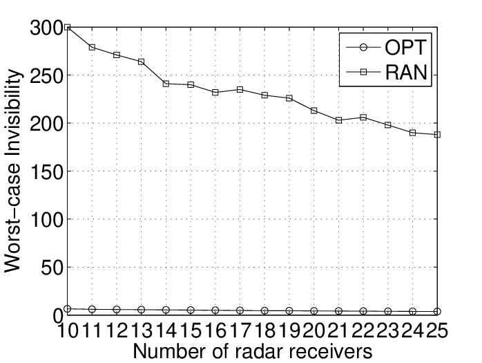
Next, we evaluate the worst-case intrusion detectability under random deployment using our proposed approximate algorithm. We consider a square field of size , where two opposite sides are entrance and destination, respectively, and the other two opposite sides are left and right boundaries, respectively. We consider deploying transmitters and receivers in the field randomly (RAN) with uniform distribution.
Figure 10, Figure 11 and Figure 12 depict the worst-case intrusion detectability versus the number of radar receivers for , , and radar transmitters, respectively, where we also plot the shortcut barrier-based optimal deployment scheme (OPT). The results for RAN are averaged over 100 simulation runs. We observe that OPT performs significantly better than RAN. The reason is that deployment on a barrier is essentially much more efficient than deployment in the full field for worst-case coverage.
6 Related Work
Worst-case coverage has been first studied in [5] for a traditional sensor network. Polynomial-time algorithms are devised to find maximum breach and maximum support paths between two locations. An efficient algorithm is proposed in [7] to solve the best-coverage problem raised in [5]. In [6], efficient algorithms are developed to find the minimum exposure path in sensor networks. Localized algorithms are designed in [11] to solve the minimum exposure path problem. A new coverage measure that captures both the best and worst-case coverage is studied in [9]. The deployment problem to improve the maximal breach path is considered by [8, 12].
Barrier coverage is an intimately related problem to worst-case coverage. The concept of weak and strong barrier coverage has been introduced in [13], where critical condition of weak barrier coverage is obtained for random deployment. The critical condition of strong barrier coverage is derived in [14] using percolation theory. An effective metric of barrier coverage quality is proposed in [15]. [16] studies constructing barrier by sensors with limited mobility after initial deployment. A novel full-view coverage model is proposed in [17] for constructing barrier in camera sensor networks.
7 Conclusion
Radar technology has great potential in many applications, such as border monitoring, security surveillance. In this paper, we studied the worst-case coverage for a bistatic radar network consisting of multiple radar transmitters and radar receivers, where each pair of radar transmitter and receiver can form a bistatic radar. The problem of optimal radar deployment is highly non-trivial since 1) the detection range of a bistatic radar is characterized by Cassini oval which presents complex geometry; 2) the detection ranges of different bistatic radars are coupled and the network coverage is intimately related to the locations of all radar nodes. We present a general assumption on the field geometry under which it is optimal to deploy radars on a shortest line segment across the field, for maximizing the worst-case intrusion detectability. Further, we characterized the corresponding optimal deployment locations along this shortest line segment. Specifically, the optimal deployment locations exhibits a balanced structure. We also developed a polynomial-time approximation algorithm for characterizing the worst-case intrusion path for any given deployment of radars.
To the best of our knowledge, the optimality of line-based deployment for the worst-case coverage, in particular for bistatic radar networks, has not been studied before this work. Although the detectability model involves some idealized assumptions, we believe that this work will be of value in setting the foundations for networked radar systems. There are still many questions remaining open for the design of networked radar.
References
- [1] N.-J. Willis, Bistatic Radar. SciTech Publishing, 2005.
- [2] C.-J. Baker and A.-L. Hume, “Netted radar sensing,” IEEE Aerospace and Electronic Systems Magazine, vol. 18, pp. 3–6, Feb. 2003.
- [3] E. Paolini, A. Giorgetti, M. Chiani, R. Minutolo, and M. Montanari, “Localization capability of cooperative anti-intruder radar systems,” EURASIP Journal on Advances in Signal Processing, 2008.
- [4] S. Bartoletti, S. Conti, and A. Giorgetti, “Analysis of uwb radar sensor networks,” in IEEE ICC 2010.
- [5] S. Meguerdichian, F. Koushanfar, M. Potkonjak, and M. Srivastava, “Coverage problems in wireless ad-hoc sensor network,” in IEEE INFOCOM 2001.
- [6] S. Meguerdichian, F. Koushanfar, G. Qu, and M. Potkonjak, “Exposure in wireless ad-hoc sensor network,” in ACM MOBICOM 2001.
- [7] X.-Y. Li, P.-J. Wan, and O. Frieder, “Coverage in wireless ad hoc sensor networks,” IEEE Transactions on Computers, vol. 52, pp. 753–763, Jun. 2003.
- [8] R.-H. Gau and Y.-Y. Peng, “A dual approach for the worst-case-coverage deployment problem in ad-hoc wireless sensor networks,” in IEEE MASS 2006.
- [9] C. Lee, D. Shin, S.-W. Bae, and S. Choi, “Best and worst-case coverage problems for arbitrary paths in wireless sensor networks,” in IEEE MASS 2010.
- [10] P. Gupta and P.-R. Kumar, “The capacity of wireless networks,” vol. 2, pp. 388–404, Mar. 2000.
- [11] S. Meguerdichian, S. Slijepcevic, V. Karayan, and M. Potkonjak, “Localized algorithms in wireless ad-hoc networks: Location discovery and sensor exposure,” in ACM MOBIHOC 2001.
- [12] A. Duttagupta, A. Bishnu, and I. Sengupta, “Optimisation problems based on the maximal breach path measure for wireless sensor network coverage,” in ICDCIT 2006.
- [13] S. Kumar, T.-H. Lai, and A. Arora, “Barrier coverage with wireless sensors,” in ACM MOBICOM 2005.
- [14] B. Liu, O. Dousse, J. Wang, and A. Saipulla, “Strong barrier coverage of wireless sensor networks,” in ACM MOBIHOC 2008.
- [15] A. Chen, T.-H. Lai, and D. Xuan, “Measuring and guaranteeing quality of barrier-coverage in wireless sensor networks,” in ACM MOBIHOC 2008.
- [16] A. Saipulla, B. Liu, G. Xing, X. Fu, and J. Wang, “Barrier coverage with sensors of limited mobility,” in ACM MOBIHOC 2010.
- [17] Y. Wang and G. Cao, “Barrier coverage in camera sensor networks,” in ACM MOBIHOC 2011.
APPENDIX
A. PROOF OF THEOREM 1
Proof: Consider any given deployment locations . It suffices to show that there exist deployment locations on such that , where ′ indicates that the deployment locations are . It follows from Property 1 that there exists a curve barrier with . Let and be the end points of curve with and . We will show that the deployment at forms a line barrier with (see Figure 13).
Let be the line passing through and . Then we can find the projection of any and onto line , denoted by and , such that and . Consider any . Since curve is a path from to , we can find a such that is the projection of onto line . Then it follows from the property of projection that and for all , . Hence, from (2) we have , and it follows that due to (5). Since is the shortcut barrier, we have . Thus, we can translate the line-based deployment onto the line where lies such that . Note that may not be all on . In this case, we can move each or to its closest end point of such that is not increased for all and hence still holds. Therefore, since is a barrier and , we have .

B. PROOF OF THEOREM 2
Proof: Consider any given deployment locations on . From the definition of barrier we have . Suppose . The proof is based on contradiction. It follows from Property 1 that there exists a barrier with . We will show that barrier must intersect with (see Figure 14).
Step 1: Consider a point with . Suppose and . Let be the line passing through such that . Consider any with . Since and for all , we have and hence . Thus intersects with at a unique point .
Step 2: Let and denote the subsets of on the left and right side of , respectively (see Figure 14). Define as an open disk centered at point with radius . We will show that and .
Let denote the circle centered at with radius . Then let denote the subset of on the left side of , which is an arc. It can be verified that and for all and for all . Then since , we have . This implies that . Similarly, we can show .
Step 3: Let and be the end points of with and . Then we have and , since otherwise or , which contradicts that is the shortcut barrier. Using the result of Step 2, we have and . Thus, curve must intersect . From the result of Step 1, must pass through . This implies that , which contradicts that .

C. PROOF OF LEMMA 1
We start with an observations which is used repeatedly in this proof. Clearly, for any , only depends on the distances of to its closest transmitter and receiver, say and , respectively. If , decreases as moves towards and ; if , since is a constant, it can be easily verified that increases as moves towards , and hence attains maximum when .
The main idea of this proof is to divide the line segment between each pair of neighbor nodes into intervals such that all points on an interval have the same pair of closest transmitter and receiver, and then we examine the structure of detectability on each interval using the observation presented above. Due to space limitation, we only prove the case when and have different types (transmitter type and receiver type) for some . The same idea is used to prove other cases.
Suppose and have different types. Without loss of generality (WLOG), let and . 1) Suppose the closest transmitter and receiver are and for any . Since for , increases as moves towards . 2) Suppose there exists some such that . Then for , and for . For each case of , increases as moves towards . Similarly, if there exists some such that , we can also show that increases as moves towards for .
D. PROOF OF LEMMA 2
Due to space limitation, we only prove the case of with pattern , and the same idea is used to prove other cases. The main idea is to determine the spacing between two neighbor nodes successively according to the given order of nodes.
Suppose and is balanced with . It follows from that . Since , given , we obtain a unique value of . Similarly, in a recursive manner, given the values of , , , we obtain a unique value of such that until we obtain a unique value of such that . Then we can see that , , , , . Similar results can be shown for any with pattern .
E. PROOF OF LEMMA 3
Due to space limitation, we only prove the case of with pattern and the same idea is used to prove other cases. Suppose and . Let denote the detectability of under . The proof is based on contradiction. Suppose . Since , we have . Using this, we can show . Then following a similar argument, using , we can show until .
Since we have supposed , we must have . It follows that , which is a contradiction. Thus we conclude . Further, it can be easily verified that if , we have , , . Similar results can be shown for any with pattern .
F. PROOF OF LEMMA 4
Suppose with any spacings. We can construct a new order of locations , from by swapping the locations of nodes and . Let denote the detectability of after the swapping. We observe that for any local vulnerable point , the closest transmitter is not , and for any local vulnerable point , . Similar observations can be made for and . Thus we can see that for any local vulnerable point or . We also observe that . Similarly, we can obtain . Furthermore, we have . Thus we have shown that for any local vulnerable point , and hence, is not increased after the swapping. Similar results can be shown for an order with any pattern given in the claim by a swapping argument.
G. PROOF OF THEOREM 3
Suppose is balanced with . We have shown that consists of a series of local suborders . Suppose is the same order as and with spacings such that , where denote the vulnerability of under . Then also consists of a series of local suborders such that and are the same local suborders for all . It is clear that , . Then Lemma 3 implies that , . Since , we must have , . Hence, by Lemma 3, we have .
H. PROOF SKETCH OF THEOREM 4
Consider any given candidate order . Clearly, consists of suborders , , where , , , , . Suppose is balanced with and .
The proof has two steps. In step 1, we suppose the conditions given in the claim do not hold, and then we can find a new order from with some spacings such that and , where denote the vulnerability of under . This implies that is no worse than . Repeating this argument, we can eventually find a new order satisfying the conditions in the claim and is no worse than . In step 2, we show that all candidate orders satisfying the conditions in the claim are equivalently good. This implies that they are all optimal orders. Due to space limitation, we only prove step 1 for the case and . The same idea is used to prove other cases in step 1 although more intricate arguments are needed for some cases.
Suppose and . Clearly, and must be local suborders. We can construct a new order from by moving a receiver from between and in to between and in . Then we set the spacings and balanced and , and we keep the spacings of any other suborder unchanged, i.e., for all . Therefore, we must have .
We observe from Lemma 2 that we have if is odd or if is even. Also, we have if is odd or if is even. Since for any , in any case, we have . Recall that we have shown . Then the desired result follows.