Recently, the ATLAS and CMS experiments at the LHC [1] have reported an excess in the gamma-gamma mode at about 125 GeV, which may be a signal of the Higgs boson. In the Standard Model (SM), a light Higgs boson is the evidence of the weakly coupled Higgs sector. In models for physics beyond the SM, however, the light Higgs boson does not always correspond to a weakly coupled theory. The scenario based on little Higgs models [2] is an example of a strongly coupled theory with a light Higgs boson, where the Higgs boson arises as a pseudo Nambu-Goldstone boson originating from the breaking of some strongly interacting global symmetry at the TeV scale, and the Higgs boson mass is kept to be light.

Supersymmetry (SUSY) is one of the most attractive candidates for the physics beyond the SM. SUSY can solve the gauge hierarchy problem, as the quadratic divergence in the radiative correction to the Higgs boson mass is cancelled owing to the non-renormalization theorem. In addition, elementary scalar fields are automatically introduced in the SUSY theory. The Higgs sector of the minimal SUSY extension of the SM (MSSM) necessarily contains two Higgs doublets. In the MSSM, the coupling constants in the Higgs potential are determined by the electroweak gauge couplings, and the mass of the SM-like Higgs boson is less than the $Z$ boson mass at the tree level. With significant radiative corrections due to the large top Yukawa coupling [3], the Higgs mass can be pushed up to around 125 GeV in the case of very large stop masses or very large left-right stop mixing.

Even within the framework based on SUSY, models with strongly coupled light Higgs boson can be constructed. A possible way is to introduce additional R-parity-even chiral superfields which strongly couple to the Higgs sector but the F-terms of which do not contribute to the Higgs boson four-point coupling. In this case, the SM-like Higgs boson is kept to be light. The strong couplings have rich phenomenological implications. First, radiative corrections involving the strongly coupled new fields can raise the SM-like Higgs boson mass to 125 GeV with rather natural choice of the stop masses and mixing. Second, the strongly coupled fields significantly contribute to the triple SM-like Higgs boson coupling through loop effects, so that it deviates by a few tens percent from the SM prediction [4, 5]. A similar non-decoupling effect tends to enhance the first order electroweak phase transition [6, 7].

In the MSSM, it is not easy to make the first order electroweak phase transition (EWPT) strong enough to satisfy the sphaleron decoupling condition [8], which is required by the successful electroweak baryogenesis [9, 10]. The non-decoupling quantum effect of the additional scalar bosons through strong F-term coupling with the Higgs boson enhances the first order EWPT, and the difficulty in the MSSM can be significantly relaxed. The enhancement requires a light SM-like Higgs boson because its mass works as a suppression factor, and the 125 GeV Higgs boson is consistent with the scenario. For example, the first order EWPT can be enough strong in a SUSY model whose Higgs sector contains four doublets and two charged singlets [7]. In this model, the coupling among the Higgs boson and the extra bosons in the scalar potential can be taken to be strong, while the quartic self-coupling constants of the Higgs boson are determined only by the D-term; i.e., by the electroweak gauge couplings, and the Higgs mass remains light.

When we explore a more fundamental picture of models with strong couplings and a light Higgs boson, a quite different landscape from the grand unified theory (GUT) over the grand desert presents itself to us. In models with strong couplings, coupling constants tend to blow up quickly through the renormalization group running. With sufficiently strong coupling consistent with successful electroweak baryogenesis, the Landau pole appears at the energy scale of multi-TeV to 10 TeV, which is much lower than the GUT scale, $O(10^{16})$ GeV. There should be a cutoff scale below the energy scale where one comes across the Landau pole. The physics above the cutoff scale might be controlled by some strong dynamics.

The minimal SUSY fat Higgs model [11] is an example of the theory above the cutoff scale of a SUSY model with strongly coupled Higgs sector. This model is based on the strong $\text{SU(2)}_{H}$ SUSY gauge theory with three pairs of doublets, $(T_{1},T_{2})$, $(T_{3},T_{4})$ and $(T_{5},T_{6})$. Below the cutoff scale, Higgs iso-spin doublets, $H_{u}$ and $H_{d}$, and a neutral singlet, $N$, appear as composite fields of $T_{i}$’s, and the other composite fields are decoupled due to their heavy masses. The low-energy effective theory is described by the superpotential $W=\lambda N(H_{d}H_{u}-v_{0}^{2})$, where $\lambda$ is a coupling constant and $v_{0}$ is a dimensionful parameter. The effective theory is identical to the nearly MSSM (nMSSM) [14]. The quartic coupling of the Higgs boson gets a $|\lambda|^{2}$ contribution through the F-term. Since the Higgs mass is dominated by the $|\lambda|^{2}v^{2}$ term with $v\simeq 174$ GeV, the strong coupling tends to enhance the Higgs mass. For $\lambda\simeq 2$ and $\tan\beta\simeq 2$, the SM-like Higgs boson mass is as large as 200 GeV, which weakens the first order EWPT too much. Extensions of the minimal SUSY fat Higgs model to $N_{c}=3,N_{f}=4$ and $N_{c}=4,N_{f}=5$ are discussed in refs. [12]. Compositeness in SUSY models is discussed in refs. [13].

In this paper, we propose a new UV-complete model whose low-energy effective theory accomodates strong couplings and a light Higgs boson. The model is based on $\text{SU}(2)_{H}$ SUSY gauge theory with three pairs of $\text{SU}(2)_{H}$ doublets. This model leads to two pairs of $Y=+1/2$ and $Y=-1/2$ iso-spin doublet composite superfields as well as several iso-spin singlet composite superfields in the low-energy description, which cause flavor changing neutral currents (FCNCs). To avoid such dangerous FCNCs, we here impose an additional $Z_{2}$ parity on the model, which is unbroken spontaneously. This $Z_{2}$ parity can supply a new candidate for dark matter, in addition to the $R$-parity. In our model, unlike the minimal SUSY fat Higgs model, the $Z_{2}$-even singlet field $N$ can be heavy enough to decouple from the low-energy effective theory, but many composite fields remain light. The Higgs sector contains two $Z_{2}$-even doublets which are identical to the MSSM-like Higgs doublets and various extra $Z_{2}$-odd superfields such as a pair of doublets, two charged singlets and two neutral singlets. The SM-like Higgs boson mass of 125 GeV can be realized in a natural way because the F-terms of the $Z_{2}$-odd superfields contribute to the mass not at the tree level but at the one-loop level. On the other hand, non-decoupling contributions of these fields in radiative corrections affect the triple Higgs boson coupling significantly [5], and can make the first order EWPT strong enough through the large F-term coupling constants [7].

In Section 2, we present the basic framework of $SU(2)_{H}$ SUSY QCD theory with the $Z_{2}$ parity, whose low-energy description gives a composite SUSY Higgs model. In Section 3, we investigate general features of the composite SUSY Higgs sector. Generally, F-terms involving a large coupling $\lambda$ contribute to the SM-like Higgs boson mass at the tree level, giving rise to a SM-like Higgs boson much heavier than 125 GeV, as in the minimal SUSY fat Higgs model. In Section 4, we consider an extended model where we obtain the SM-like Higgs boson as light as 125 GeV in a natural way. It turns out that its low-energy effective theory describes the phenomenological model in ref. [7]. Section 5 is devoted to the conclusion.

We introduce a new $SU(2)$ gauge group, denoted by $SU(2)_{H}$, and six chiral superfields, denoted by $T_{i}\ (i=1,2,...,6)$, which are doublets of $SU(2)_{H}$. $T_{i}$’s are also charged under SM gauge groups $SU(2)_{L}\times U(1)_{Y}$. We further assign a $Z_{2}$ parity to them. SM charge and $Z_{2}$ parity assignments to $T_{i}$’s are described in Table 1.

Regarding $SU(2)_{H}$ gauge group, this model is nothing but the SUSY QCD theory with 2 colors and 3 flavors, which is investigated in ref. [15]. $SU(2)_{H}$ gauge coupling becomes strong at an infrared scale, denoted by $\Lambda_{H}$. The most general tree-level superpotential that is invariant under $SU(2)_{H}\times SU(2)_{L}\times U(1)_{Y}\times Z_{2}$ symmetry is given by

	$\displaystyle W_{tree}$	$\displaystyle=$	$\displaystyle\frac{1}{2}m_{1}\ {\rm tr}\left[\left(\begin{array}[]{cc}T^{2}_{2}&-T^{1}_{2}\\ -T^{2}_{1}&T^{1}_{1}\end{array}\right)\left(\begin{array}[]{cc}T^{1}_{1}&T^{1}_{2}\\ T^{2}_{1}&T^{2}_{2}\end{array}\right)\right]\ +\ m_{3}T_{3}T_{4}\ +\ m_{5}T_{5}T_{6}$		(6)
		$\displaystyle=$	$\displaystyle m_{1}T_{1}T_{2}\ +\ m_{3}T_{3}T_{4}\ +\ m_{5}T_{5}T_{6}\ ,$

where we assume $m_{1},m_{3},m_{5}<\Lambda_{H}$ so that the theory remains the SUSY QCD theory with $N_{c}=2$ and $N_{f}=3$ at the scale $\Lambda_{H}$. $T^{a}_{1}$ and $T^{a}_{2}\ (a=1,2)$ respectively indicate the $a$-th components of the $SU(2)_{H}$ doublets $T_{1}$ and $T_{2}$. In the right hand side of the first line, the first matrix transforms as $(2^{*},2^{*})$ and the second one does as $(2,2)$ under $SU(2)_{H}\times SU(2)_{L}$. The trace of their product is thus invaraint under $SU(2)_{H}\times SU(2)_{L}$.

Below $\Lambda_{H}$, the theory is described in terms of composite chiral superfields, $M_{ij}^{\prime}=T_{i}T_{j}\ (i\neq j)$, which are singlets of $SU(2)_{H}$. Following the arguments in ref. [15], we see that we have the following dynamically generated superpotential below $\Lambda_{H}$:

$\displaystyle W_{dyn}$

$\displaystyle=$

$\displaystyle-\frac{1}{\Lambda^{3}}\ \epsilon^{ijklmn}\ M_{ij}^{\prime}M_{kl}^{\prime}M_{mn}^{\prime}\ ,$

(7)

where $\Lambda$ is some dynamically generated scale. Thanks to holomorphy, the net effective superpotential is simply the sum of $W_{dyn}$ and $W_{tree}$:

	$\displaystyle W_{eff}$	$\displaystyle=$	$\displaystyle W_{dyn}\ +\ W_{tree}$		(8)
		$\displaystyle=$	$\displaystyle W_{dyn}\ +\ m_{1}M_{12}^{\prime}\ +\ m_{3}M_{34}^{\prime}\ +\ m_{5}M_{56}^{\prime}\ .$

Since we cannot determine the Kähler potential only from holomorphy, we take advantage of Na$\ddot{\char 16\relax}$ve Dimensional Analysis (NDA) [16]. Before using NDA, we note that the terms in $W_{tree}$ are exactly proportional to $m_{1}/\Lambda_{H}$, $m_{3}/\Lambda_{H}$, $m_{5}/\Lambda_{H}$ because of holomorphy. In NDA, it is assumed that the other couplings in the effective Lagrangian are $O(1)$ in unit of $\Lambda_{H}$ and that the effective theory also becomes strongly coupled at the scale $\Lambda_{H}$. Therefore the effective Lagrangian at $\Lambda_{H}$ is expressed as

	$\displaystyle{\cal L}_{eff}$	$\displaystyle\simeq$	$\displaystyle\frac{1}{(4\pi)^{2}}\ \left[\ \int{\rm d}^{4}\theta\ \Lambda_{H}^{2}\ \hat{K}\left(\frac{M^{\prime}}{\Lambda_{H}^{2}},\frac{D^{\alpha}}{\Lambda_{H}},\frac{M^{\prime\,\dagger}}{\Lambda_{H}^{2}},\frac{\bar{D}_{\dot{\alpha}}}{\Lambda_{H}}\right)\right.$
		$\displaystyle+$	$\displaystyle\left.\int{\rm d}^{2}\theta\ \Lambda_{H}^{3}\ \left\{\ \hat{W}\left(\frac{M^{\prime}}{\Lambda_{H}^{2}},\frac{D^{\alpha}}{\Lambda_{H}}\right)\ +\ \frac{m_{1}}{\Lambda_{H}}\frac{M_{12}^{\prime}}{\Lambda_{H}^{2}}\ +\ \frac{m_{3}}{\Lambda_{H}}\frac{M_{34}^{\prime}}{\Lambda_{H}^{2}}\ +\ \frac{m_{5}}{\Lambda_{H}}\frac{M_{56}^{\prime}}{\Lambda_{H}^{2}}\ \right\}\ +{\rm h.c.}\ \right]\ ,$

where the SM gauge interactions are omitted. We rewrite the theory in terms of canonically normalized composite fields, $M_{ij}$, which are given by

$\displaystyle M_{ij}$

$\displaystyle\simeq$

$\displaystyle\frac{1}{4\pi\Lambda_{H}}M^{\prime}_{ij}\ \ \ {\rm at\ the\ scale}\ \Lambda_{H}\ ,$

(10)

and obtain the following canonical effective superpotential below $\Lambda_{H}$ expressed in terms of $M_{ij}$’s:

$\displaystyle W_{eff}$

$\displaystyle\simeq$

$\displaystyle-\lambda\ \epsilon^{ijklmn}\ M_{ij}M_{kl}M_{mn}\ +\ \xi_{\Omega}M_{12}\ +\ \xi_{\Phi}M_{34}\ +\ \xi M_{56}\ ,$

(11)

where $\lambda,\ \xi_{\Omega},\ \xi_{\Phi},\ \xi$ satisfy at the scale $\Lambda_{H}$

	$\displaystyle\lambda(\Lambda_{H})$	$\displaystyle\simeq$	$\displaystyle 4\pi\ ,$		(12)
	$\displaystyle\xi_{\Omega}(\Lambda_{H})$	$\displaystyle\simeq$	$\displaystyle\frac{m_{1}\Lambda_{H}}{4\pi}\ ,\ \ \ \xi_{\Phi}(\Lambda_{H})\ \simeq\ \frac{m_{3}\Lambda_{H}}{4\pi}\ ,\ \ \ \xi(\Lambda_{H})\ \simeq\ \frac{m_{5}\Lambda_{H}}{4\pi}\ .$		(13)

Below the scale $\Lambda_{H}$, the physical couplings that correspond to $\lambda,\ \xi_{\Omega},\ \xi_{\Phi},\ \xi$ are regulated by the following renormalization group equations:

	$\displaystyle\mu\frac{{\rm d}}{{\rm d}\mu}\left(\frac{1}{\lambda^{2}}\right)$	$\displaystyle\simeq$	$\displaystyle-\frac{9}{16\pi^{2}}\ ,$		(14)
	$\displaystyle\mu\frac{{\rm d}}{{\rm d}\mu}\xi$	$\displaystyle\simeq$	$\displaystyle\frac{3}{32\pi^{2}}\lambda^{2}\ \xi\ ,\ \ \ \mu\frac{{\rm d}}{{\rm d}\mu}\xi_{\Phi}\ \simeq\ \frac{3}{32\pi^{2}}\lambda^{2}\ \xi_{\Phi}\ ,\ \ \ \mu\frac{{\rm d}}{{\rm d}\mu}\xi_{\Omega}\ \simeq\ \frac{3}{32\pi^{2}}\lambda^{2}\ \xi_{\Omega}\ .$		(15)

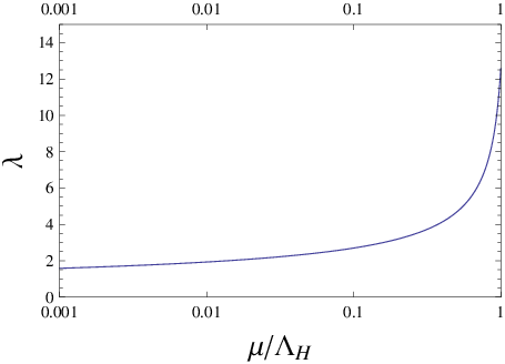
Figure 1 shows the renormalization group running of the physical coupling $\lambda$ from the scale $\Lambda_{H}$ to lower scales. For example, if $\Lambda_{H}\simeq 10$ TeV, $\lambda$ at the scale $M_{Z}$ is $\sim 2$. The runnings of $\xi_{\Omega},\ \xi_{\Phi},\ \xi$ are not so drastic and can be neglected.

We rewrite the composite superfields $M_{ij}$ in the following way to clarify their SM charges:

	$\displaystyle H_{u}$	$\displaystyle\equiv$	$\displaystyle\left(\begin{array}[]{c}M_{13}\\ M_{23}\end{array}\right)\ ,\ \ \ H_{d}\ \equiv\ \left(\begin{array}[]{c}M_{14}\\ M_{24}\end{array}\right)\ ,\ \ \ \Phi_{u}\ \equiv\ \left(\begin{array}[]{c}M_{15}\\ M_{25}\end{array}\right)\ ,\ \ \ \Phi_{d}\ \equiv\ \left(\begin{array}[]{c}M_{16}\\ M_{26}\end{array}\right)\ ,\ \ \$
	$\displaystyle N$	$\displaystyle\equiv$	$\displaystyle M_{56}\ ,\ \ \ N_{\Phi}\ \equiv\ M_{34}\ ,\ \ \ N_{\Omega}\ \equiv\ M_{12}\ ,\ \ \$
	$\displaystyle\Omega^{+}$	$\displaystyle\equiv$	$\displaystyle M_{35}\ ,\ \ \ \Omega^{-}\ \equiv\ M_{46}\ ,\ \ \ \zeta\ \equiv\ M_{36}\ ,\ \ \ \eta\ \equiv\ M_{45}\ .\ \ \$		(25)

Their SM charges and $Z_{2}$-parities are summarized in Table 2.

The effective superpotential is then written as

	$\displaystyle W_{eff}$	$\displaystyle=$	$\displaystyle\lambda\ \left\{\ N(H_{u}H_{d}+v_{0}^{2})\ +\ N_{\Phi}(\Phi_{u}\Phi_{d}+v_{\Phi}^{2})\ +\ N_{\Omega}(\Omega^{+}\Omega^{-}+v_{\Omega}^{2})\right.$		(26)
		$\displaystyle-$	$\displaystyle\left.NN_{\Phi}N_{\Omega}\ -\ N_{\Omega}\zeta\eta\ +\ \zeta H_{d}\Phi_{u}\ +\ \eta H_{u}\Phi_{d}\ -\ \Omega^{+}H_{d}\Phi_{d}\ -\ \Omega^{-}H_{u}\Phi_{u}\ \right\}\ ,$

where $v_{0}^{2},\ v_{\Phi}^{2},\ v_{\Omega}^{2}$ are defined as

$\displaystyle v_{0}^{2}$

$\displaystyle\equiv$

$\displaystyle\xi/\lambda\ ,\ \ \ v_{\Phi}^{2}\ \equiv\ \xi_{\Phi}/\lambda\ ,\ \ \ v_{\Omega}^{2}\ \equiv\ \xi_{\Omega}/\lambda\ .$

(27)

We note that all the three-point couplings are of the same magnitude in this model.

First of all, we look for vacua of the Higgs potential in the effective theory. We study in the SUSY limit and then with soft SUSY breaking terms. In the SUSY limit, the absolute minima of the superpotential (12) are determined from the tadpole conditions: $(\partial/\partial\phi)W_{eff}=0$ for each field $\phi$ at the tree level. Since we are only interested in charge-conserving vacua, we set $H_{u}^{+}=H_{d}^{-}=\Phi_{u}^{+}=\Phi_{d}^{-}=\Omega^{+}=\Omega^{-}=0$ and study whether the tadpole conditions can be satisfied. Charge-conserving vacua are determined from the following tadpole conditions:

	$\displaystyle 0$	$\displaystyle=$	$\displaystyle\frac{1}{\lambda}\frac{\partial W_{eff}}{\partial N_{\Omega}}\ =\ -NN_{\Phi}-\zeta\eta+v_{\Omega}^{2}\ ,$		(28)
	$\displaystyle 0$	$\displaystyle=$	$\displaystyle\frac{1}{\lambda}\frac{\partial W_{eff}}{\partial N}\ =\ -H_{u}^{0}H_{d}^{0}-N_{\Omega}N_{\Phi}+v_{0}^{2}\ ,$		(29)
	$\displaystyle 0$	$\displaystyle=$	$\displaystyle\frac{1}{\lambda}\frac{\partial W_{eff}}{\partial N_{\Phi}}\ =\ -\Phi_{u}^{0}\Phi_{d}^{0}-N_{\Omega}N+v_{\Phi}^{2}\ ,$		(30)
	$\displaystyle 0$	$\displaystyle=$	$\displaystyle\frac{1}{\lambda}\frac{\partial W_{eff}}{\partial\zeta}\ =\ H_{d}^{0}\Phi_{u}^{0}-N_{\Omega}\eta\ ,$		(31)
	$\displaystyle 0$	$\displaystyle=$	$\displaystyle\frac{1}{\lambda}\frac{\partial W_{eff}}{\partial\eta}\ =\ -H_{u}^{0}\Phi_{d}^{0}-N_{\Omega}\zeta\ ,$		(32)
	$\displaystyle 0$	$\displaystyle=$	$\displaystyle\frac{1}{\lambda}\frac{\partial W_{eff}}{\partial H_{u}^{0}}\ =\ -NH_{d}^{0}-\eta\Phi_{d}^{0}\ ,$		(33)
	$\displaystyle 0$	$\displaystyle=$	$\displaystyle\frac{1}{\lambda}\frac{\partial W_{eff}}{\partial\Phi_{u}^{0}}\ =\ -N_{\Phi}\Phi_{d}^{0}+\zeta H_{d}^{0}\ ,$		(34)
	$\displaystyle 0$	$\displaystyle=$	$\displaystyle\frac{1}{\lambda}\frac{\partial W_{eff}}{\partial H_{d}^{0}}\ =\ -NH_{u}^{0}+\zeta\Phi_{u}^{0}\ ,$		(35)
	$\displaystyle 0$	$\displaystyle=$	$\displaystyle\frac{1}{\lambda}\frac{\partial W_{eff}}{\partial\Phi_{d}^{0}}\ =\ -N_{\Phi}\Phi_{u}^{0}-\eta H_{u}^{0}\ ,$		(36)
	$\displaystyle 0$	$\displaystyle=$	$\displaystyle D\ =\ -\frac{1}{2}g_{1}\ (H_{u}^{0\,\dagger}H_{u}^{0}-H_{d}^{0\,\dagger}H_{d}^{0})\ -\ \frac{1}{2}g_{1}\ (\Phi_{u}^{0\,\dagger}\Phi_{u}^{0}-\Phi_{d}^{0\,\dagger}\Phi_{d}^{0})\ ,$		(37)
	$\displaystyle 0$	$\displaystyle=$	$\displaystyle D^{a=3}\ =\ -\frac{1}{2}g_{2}\ (-H_{u}^{0\,\dagger}H_{u}^{0}+H_{d}^{0\,\dagger}H_{d}^{0})\ -\ \frac{1}{2}g_{2}\ (-\Phi_{u}^{0\,\dagger}\Phi_{u}^{0}+\Phi_{d}^{0\,\dagger}\Phi_{d}^{0})\ ,$		(38)

Since no symmetry forbids the term $m_{1}T_{1}T_{2}$ in the fundamental Lagrangian, we assume $v_{\Omega}^{2}\neq 0$. Then the only solution to eqs. (14) and (19)-(22) is $H_{d}^{0}=\Phi_{d}^{0}=H_{u}^{0}=\Phi_{u}^{0}=0$, i.e. the electroweak symmetry is unbroken in the absolute SUSY vacua. At this point, our model distinctively differs from the minimal SUSY fat Higgs model [11], where non-anomalous $U(1)_{R}$ charges are assigned to forbid the term $m_{1}T_{1}T_{2}$ so that the electroweak symmetry breaking does occur in the SUSY limit. The D-terms are all zero in the absolute SUSY vacua because we have $H_{d}^{0}=\Phi_{d}^{0}=H_{u}^{0}=\Phi_{u}^{0}=0$. The conditions in eqs. (14)-(16) determine the VEVs of $N,N_{\Phi}$ and $N_{\Omega}$ as follows :

$\displaystyle\langle N\rangle\langle N_{\Phi}\rangle$

$\displaystyle=$

$\displaystyle v_{\Omega}^{2},\ \ \ \langle N_{\Omega}\rangle\langle N_{\Phi}\rangle\ =\ v_{0}^{2},\ \ \ \langle N_{\Omega}\rangle\langle N\rangle\ =\ v_{\Phi}^{2}\ .$

(39)

We assume $v_{0}^{2}\neq 0$ and $v_{\Phi}^{2}\neq 0$ as no symmetry forbids these terms. We then have $\langle N_{\Omega}\rangle\neq 0$, which leads to $\eta=\zeta=0$ through eqs. (17) and (18). Note that the $Z_{2}$ parity is unbroken in the absolute SUSY vacua.

Since the conditions in eq. (25) have only one solution and the other neutral components are derived to be zero, we conclude that there is only one charge-conserving absolute SUSY vacuum provided $v_{0}^{2},\ v_{\Phi}^{2}$ and $v_{\Omega}^{2}$ are all non-zero. This vacuum respects the electroweak symmetry and the $Z_{2}$ parity. The non-zero VEVs of $N,\ N_{\Phi}$ and $N_{\Omega}$ give rise to effective $\mu$-terms.

Let us proceed to the case with soft SUSY breaking terms. For simplicity, we only introduce soft SUSY breaking mass terms and $B\mu$-term for $H_{u}$ and $H_{d}$, which we denote by $m_{H_{u}}^{2},\ m_{H_{d}}^{2}$ and $B\mu$. We redefine the phases of $T_{3}$ and $T_{5}$ to make $B\mu$ and $v_{0}^{2}$ real and positive. We further rotate the phase of $(T_{1},T_{2})$ so that the product of the VEVs of $N_{\Phi}$ and $N_{\Omega}$ is real. We expand the potential with respect to $H_{u},H_{d},N,N_{\Omega}$ and $N_{\Phi}$, with setting $\Phi_{u}=\Phi_{d}=\Omega^{+}=\Omega^{-}=\zeta=\eta=0$. The tree-level potential is then expressed as

	$\displaystyle V$	$\displaystyle=$	$\displaystyle m_{H_{u}}^{2}H_{u}^{\dagger}H_{u}\ +\ m_{H_{d}}^{2}H_{d}^{\dagger}H_{d}\ +\ B\mu H_{u}H_{d}\ +\ h.c.$		(40)
		$\displaystyle+$	$\displaystyle|\lambda|^{2}|N|^{2}(|H_{u}|^{2}+|H_{d}|^{2})$
		$\displaystyle+$	$\displaystyle|\lambda|^{2}|H_{u}H_{d}-N_{\Phi}N_{\Omega}+v_{0}^{2}|^{2}$
		$\displaystyle+$	$\displaystyle|\lambda|^{2}|NN_{\Omega}-v_{\Phi}^{2}|^{2}\ +\ |\lambda|^{2}|NN_{\Phi}-v_{\Omega}^{2}|^{2}$
		$\displaystyle+$	$\displaystyle\frac{1}{8}g_{1}^{2}\ (H_{u}^{\dagger}H_{u}-H_{d}^{\dagger}H_{d})^{2}\ +\ \frac{1}{8}g_{2}^{2}\ (H_{u}^{\dagger}\sigma^{a}H_{u}+H_{d}^{\dagger}\sigma^{a}H_{d})^{2}\ .$

Using the $SU(2)_{L}$ gauge symmetry, we take $H_{u}^{+}=0$. Then the condition: $(\partial/\partial H_{u}^{+})V=0$ leads to $H_{d}^{-}=0$, as in the MSSM. From the conditions: $(\partial/\partial H_{u}^{0\,*})V=(\partial/\partial H_{d}^{0\,*})V=(\partial/\partial H_{u}^{0})V=(\partial/\partial H_{d}^{0})V=0$, we have

	$\displaystyle\frac{1}{4}(g_{1}^{2}+g_{2}^{2})(|H_{u}^{0}|^{2}-|H_{d}^{0}|^{2})H_{u}^{0}$	$\displaystyle+$	$\displaystyle(m_{H_{u}}^{2}+|\lambda|^{2}|N|^{2}+|\lambda|^{2}|H_{d}^{0}|^{2})H_{u}^{0}$		(41)
		$\displaystyle+$	$\displaystyle(|\lambda|^{2}N_{\Phi}N_{\Omega}-|\lambda|^{2}v_{0}^{2}-B\mu)H_{d}^{0\,*}\ =\ 0\ ,$
	$\displaystyle-\frac{1}{4}(g_{1}^{2}+g_{2}^{2})(|H_{u}^{0}|^{2}-|H_{d}^{0}|^{2})H_{u}^{0}$	$\displaystyle+$	$\displaystyle(m_{H_{d}}^{2}+|\lambda|^{2}|N|^{2}+|\lambda|^{2}|H_{u}^{0}|^{2})H_{d}^{0}$		(42)
		$\displaystyle+$	$\displaystyle(|\lambda|^{2}N_{\Phi}N_{\Omega}-|\lambda|^{2}v_{0}^{2}-B\mu)H_{u}^{0\,*}\ =\ 0\ ,$
	$\displaystyle H_{u}^{0}H_{d}^{0}$	$\displaystyle=$	$\displaystyle{\rm real}\ ,$		(43)

by using the fact that $B\mu$, $v_{0}^{2}$ and the VEV of $N_{\Phi}N_{\Omega}$ are real. Since the VEV of $H_{u}^{0}H_{d}^{0}$ is real, we can take the VEVs of $H_{u}^{0}$ and $H_{d}^{0}$ both real by using the $U(1)_{Y}$ gauge symmetry. We hereafter denote these VEVs by $v_{u}$ and $v_{d}$, respectively. The conditions: $(\partial/\partial N)V=(\partial/\partial N_{\Phi})V=(\partial/\partial N_{\Omega})V=0$ and their complex conjugates lead to

	$\displaystyle N(v_{u}^{2}+v_{d}^{2})\ +\ N_{\Omega}^{*}(NN_{\Omega}-v_{\Phi}^{2})\ +\ N_{\Phi}^{*}(NN_{\Phi}-v_{\Omega}^{2})$	$\displaystyle=$	$\displaystyle 0\ ,$		(44)
	$\displaystyle N_{\Omega}^{*}(N_{\Phi}N_{\Omega}+v_{u}v_{d}-v_{0}^{2})\ +\ N^{*}(NN_{\Phi}-v_{\Omega}^{2})$	$\displaystyle=$	$\displaystyle 0\ ,$		(45)
	$\displaystyle N_{\Phi}^{*}(N_{\Phi}N_{\Omega}+v_{u}v_{d}-v_{0}^{2})\ +\ N^{*}(NN_{\Omega}-v_{\Phi}^{2})$	$\displaystyle=$	$\displaystyle 0\ ,$		(46)
	$\displaystyle N^{*}N_{\Phi}^{*}v_{\Omega}^{2},\ N^{*}N_{\Omega}^{*}v_{\Phi}^{2}$	$\displaystyle=$	$\displaystyle{\rm real}\ .$		(47)

We derive the mass spectrum in the presence of soft SUSY breaking terms. For simplicity, we here assume that $v_{\Phi}^{2}$ and $v_{\Omega}^{2}$ are also real and positive. We assume that $|v_{u}|,|v_{d}|\ll\sqrt{v_{0}^{2}},\sqrt{v_{\Phi}^{2}},\sqrt{v_{\Omega}^{2}}$ and we make a perturbative expansion of the masses with respect to $v_{u}^{2}$ and $v_{d}^{2}$. At the zeroth order of $v_{u}^{2}$ and $v_{d}^{2}$, the VEVs of $N,N_{\Phi}$ and $N_{\Omega}$, denoted by $\langle N\rangle^{0},\ \langle N_{\Phi}\rangle^{0}$ and $\langle N_{\Omega}\rangle^{0}$, are given by

$\displaystyle\langle N\rangle^{0}$

$\displaystyle=$

$\displaystyle\sqrt{\frac{v_{\Phi}^{2}v_{\Omega}^{2}}{v_{0}^{2}}}\ ,\ \ \ \langle N_{\Phi}\rangle^{0}\ =\ \sqrt{\frac{v_{0}^{2}v_{\Omega}^{2}}{v_{\Phi}^{2}}}\ ,\ \ \ \langle N_{\Omega}\rangle^{0}\ =\ \sqrt{\frac{v_{0}^{2}v_{\Phi}^{2}}{v_{\Omega}^{2}}}\ ,$

(48)

which are the same as those in the SUSY limit. These VEVs respectively correspond to the SUSY-conserving masses of $(H_{u},H_{d})$, $(\Phi_{u},\Phi_{d})$ and $(\Omega^{+},\Omega^{-})$. In the following discussion, we use the VEVs of $N^{0},N_{\Phi}^{0}$ and $N_{\Omega}^{0}$ as the parameters of the model, instead of $v_{0}^{2},v_{\Phi}^{2}$ and $v_{\Omega}^{2}$. The VEVs of $N,N_{\Phi}$ and $N_{\Omega}$ at the first order of $v_{u}^{2}$ and $v_{d}^{2}$, denoted by $\langle N\rangle^{1},\langle N_{\Phi}\rangle^{1}$ and $\langle N_{\Omega}\rangle^{1}$, satisfy the following relations:

			$\displaystyle\left(\begin{array}[]{ccc}(\langle N_{\Phi}\rangle^{0})^{2}+(\langle N_{\Omega}\rangle^{0})^{2}&\langle N\rangle^{0}\langle N_{\Phi}\rangle^{0}&\langle N\rangle^{0}\langle N_{\Omega}\rangle^{0}\\ &(\langle N\rangle^{0})^{2}+(\langle N_{\Omega}\rangle^{0})^{2}&\langle N_{\Phi}\rangle^{0}\langle N_{\Omega}\rangle^{0}\\ &&(\langle N\rangle^{0})^{2}+(\langle N_{\Phi}\rangle^{0})^{2}\end{array}\right)\left(\begin{array}[]{c}\langle N\rangle^{1}\\ \langle N_{\Phi}\rangle^{1}\\ \langle N_{\Omega}\rangle^{1}\end{array}\right)$
		$\displaystyle=$	$\displaystyle\left(\begin{array}[]{c}-\langle N\rangle^{0}(v_{u}^{2}+v_{d}^{2})\\ 0\\ 0\end{array}\right)\ .$

We next study the mass spectrum of the $Z_{2}$-even Higgs sector. At the first order of $v_{u}^{2}$ and $v_{d}^{2}$, the conditions (26) and (27) reduce to

	$\displaystyle\frac{1}{4}(g_{1}^{2}+g_{2}^{2})(v_{u}^{2}-v_{d}^{2})v_{u}$	$\displaystyle+$	$\displaystyle(\ m_{H_{u}}^{2}+|\lambda|^{2}|\langle N\rangle^{0}+\langle N\rangle^{1}|^{2}+|\lambda|^{2}v_{d}^{2}\ )\ v_{u}$
		$\displaystyle+$	$\displaystyle\{\ |\lambda|^{2}\ (\ \langle N_{\Phi}\rangle^{1}\langle N_{\Omega}\rangle^{0}+\langle N_{\Phi}\rangle^{0}\langle N_{\Omega}\rangle^{1}\ )\ -\ B\mu\ \}\ v_{d}\ =\ 0\ ,$
	$\displaystyle-\frac{1}{4}(g_{1}^{2}+g_{2}^{2})(v_{u}^{2}-v_{d}^{2})v_{d}$	$\displaystyle+$	$\displaystyle(\ m_{H_{d}}^{2}+|\lambda|^{2}|\langle N\rangle^{0}+\langle N\rangle^{1}|^{2}+|\lambda|^{2}v_{u}^{2}\ )\ v_{d}$
		$\displaystyle+$	$\displaystyle\{\ |\lambda|^{2}\ (\ \langle N_{\Phi}\rangle^{1}\langle N_{\Omega}\rangle^{0}+\langle N_{\Phi}\rangle^{0}\langle N_{\Omega}\rangle^{1}\ )\ -\ B\mu\ \}\ v_{u}\ =\ 0\ .$

They give the same conditions for the electroweak symmetry breaking as in the Next-to-MSSM [18] if we define the effective $B\mu$-term as

$\displaystyle B\mu_{eff}$

$\displaystyle\equiv$

$\displaystyle B\mu\ -\ |\lambda|^{2}\ (\ \langle N_{\Phi}\rangle^{1}\langle N_{\Omega}\rangle^{0}+\langle N_{\Phi}\rangle^{0}\langle N_{\Omega}\rangle^{1}\ )\ .$

(62)

We comment on the range of $\Lambda_{H}$ favored by the naturalness. NDA implies that the Lagrangian contains the following Kähler potential:

$\displaystyle{\cal L}_{eff}$

$\displaystyle\supset$

$\displaystyle\int{\rm d}^{4}\theta\ \frac{\Lambda_{H}}{4\pi}\ (\ N+N_{\Phi}+N_{\Omega}\ )\$

(63)

with a $O(1)$ factor for each coupling. We now turn on the effects of soft SUSY breaking. We introduce a singlet chiral superfield $X$ whose F-term, $F_{X}$, has a non-zero VEV. We couple $X$ to the other superfields by contact interactions suppressed by the scale $M$, where $M$ is indentified with the Planck scale in the case of gravity mediation and with the messenger scale in the case of gauge mediation ¹¹ 1 Notice that since the superfields $N,N_{\Phi}$ and $N_{\Omega}$ are composites of the fundamental superfields $T_{i}$’s, which are charged under the $SU(2)_{H}$ gauge group, gauge mediation can induce soft SUSY breaking terms for $N,N_{\Phi}$ and $N_{\Omega}$ even if they are gauge singlets.. The soft SUSY breaking scale is given by $F_{X}/M$. With soft SUSY breaking effects, we have the following Kähler potential that gives extra contributions to the tadpole terms in eq. (6):

	$\displaystyle{\cal L}_{eff}$	$\displaystyle\supset$	$\displaystyle\int{\rm d}^{4}\theta\ \frac{X^{\dagger}}{M}\ \frac{\Lambda_{H}}{4\pi}\ (\ N+N_{\Phi}+N_{\Omega}\ )\ +\ {\rm h.c.}$		(64)
		$\displaystyle=$	$\displaystyle\frac{F_{X}^{\dagger}}{M}\ \int{\rm d}^{2}\theta\ \frac{\Lambda_{H}}{4\pi}\ (\ N+N_{\Phi}+N_{\Omega}\ )\ +\ {\rm h.c.}\ .$

These extra contributions affect the VEV of $N$, which is given by

$\displaystyle\langle N\rangle$

$\displaystyle=$

$\displaystyle\sqrt{\frac{1}{\lambda(M_{Z})}}\sqrt{\frac{\xi^{\prime}_{\Phi}\ \xi^{\prime}_{\Omega}}{\xi^{\prime}}}\ ,$

(65)

where $\xi^{\prime},\xi^{\prime}_{\Phi}$ and $\xi^{\prime}_{\Omega}$ are the sums of the tadpoles in eq. (6) and the extra contributions from soft SUSY breaking effects, which are expressed as

$\displaystyle\xi^{\prime}$

$\displaystyle=$

$\displaystyle\xi\ +\ a\frac{F_{X}^{\dagger}}{M}\frac{\Lambda_{H}}{4\pi}\ ,\ \ \ \xi_{\Phi}^{\prime}\ =\ \xi_{\Phi}\ +\ a_{\Phi}\frac{F_{X}^{\dagger}}{M}\frac{\Lambda_{H}}{4\pi}\ ,\ \ \ \xi_{\Omega}^{\prime}\ =\ \xi_{\Omega}\ +\ a_{\Omega}\frac{F_{X}^{\dagger}}{M}\frac{\Lambda_{H}}{4\pi}\ ,$

(66)

where $a,a_{\Phi}$ and $a_{\Omega}$ are all $O(1)$. On the other hand, to break the electroweak symmetry without unnatural cancellation between the effective $\mu$-term $\lambda(M_{Z})\langle N\rangle$ and the soft SUSY breaking terms $m_{H_{u}}^{2}$ and $m_{H_{d}}^{2}$, we require that $\lambda(M_{Z})\langle N\rangle$ be smaller than about 1 TeV, which is equivalent to

$\displaystyle\sqrt{\frac{\xi^{\prime}_{\Phi}\ \xi^{\prime}_{\Omega}}{\xi^{\prime}}}$

$\displaystyle\lesssim$

$\displaystyle\frac{1}{\sqrt{\lambda(M_{Z})}}\ \times\ 1\ {\rm TeV}\ .$

(67)

To satisfy the above condition in the presence of soft SUSY breaking effects, it is required that

$\displaystyle\sqrt{\left|\frac{F_{X}}{M}\right|\frac{\Lambda_{H}}{4\pi}}$

$\displaystyle\lesssim$

$\displaystyle\frac{1}{\sqrt{\lambda(M_{Z})}}\ \times\ 1\ {\rm TeV}\ .$

(68)

Assuming that the soft SUSY breaking scale $F_{X}/M$ is about 1 TeV and $\lambda(M_{Z})$ is $O(1)$, we obtain the following estimate on the upper bound of $\Lambda_{H}$ suggested by the naturalness:

$\displaystyle\Lambda_{H}$

$\displaystyle\lesssim$

$\displaystyle 4\pi\ \times\ 1\ {\rm TeV}\ .$

(69)

Now that we know the favorable range of $\Lambda_{H}$, we discuss the mass of the SM-like Higgs boson, $m_{h}$, which depends on $\Lambda_{H}$ via $\lambda(M_{Z})$. In the decoupling limit, $m_{h}$ is given at the tree level by [18]

$\displaystyle m_{h}^{2}$

$\displaystyle\simeq$

$\displaystyle M_{Z}^{2}\cos^{2}(2\beta)\ +\ \lambda(M_{Z})^{2}v^{2}\sin^{2}(2\beta)\ .$

(70)

Here we introduce $\tan\beta\equiv v_{u}/v_{d}$ as usual. Since the naturalness suggests $\Lambda_{H}\lesssim 10$ TeV, we have $\lambda(M_{Z})>1.9$, according to Figure 1. Therefore, to realize the Higgs boson mass of $125$ GeV, we need large $\tan\beta$ so that the contribution from the second term in eq. (46) is suppressed.

Finally we comment on how the SM Yukawa couplings of appropriate magnitudes can be derived in this model, especially for the $O(1)$ top quark Yukawa coupling. We adopt the mechanism proposed in refs. [17, 11]. First we introduce two additional $SU(2)_{H}$ doublets, $T_{7}$ and $T_{8}$, which have the tree-level mass term below:

$\displaystyle W_{7}$

$\displaystyle=$

$\displaystyle m_{7}T_{7}T_{8}\ ,$

(71)

where $m_{7}>\Lambda_{H}$ is assumed. Above the scale $m_{7}$, our model is described by the SUSY QCD theory with two colors and four flavors and is in the superconformal window. We assume that this theory approaches the infrared fixed point at some scale $\Lambda_{4}>m_{7}$ and becomes nearly conformal. At the scale $m_{7}$, the fields $T_{7}$ and $T_{8}$ decouple and the theory becomes the SUSY QCD theory with two colors and three flavors. Through renormalization group evolutions, the wavefunctions of $T_{i}$’s receive large corrections of

$\displaystyle Z$

$\displaystyle\simeq$

$\displaystyle\left(\frac{m_{7}}{\Lambda_{4}}\right)^{\gamma^{*}}\ ,$

(72)

where $\gamma^{*}$ denotes the anomalous dimension at the infrared fixed point, which equals to $(3N_{c}-N_{f})/N_{f}=1/2$ for the $N_{c}=2$ and $N_{f}=4$ SUSY QCD theory. By introducing new $SU(2)_{H}$ singlets with SUSY-conserving mass $M_{f}\sim\Lambda_{H}$ and integrating them out, it is possible to have the following higher-dimensional superpotential at the scale $\Lambda_{H}$:

$\displaystyle W_{f}$

$\displaystyle=$

$\displaystyle\frac{1}{M_{f}}Z^{-1}h_{u}^{ij}(T_{1}T_{3},T_{2}T_{3})Q_{i}U_{j}\ +\ \cdots,$

(73)

where $h_{u}^{ij}$ denotes the Yukawa coupling in the fundamental theory, whose value is at most $O(1)$ and the factor of $Z^{-1}$ comes from the wavefunction renormalization of $T_{i}$’s. Therefore the fundamental theory may not contain any Landau pole below the Planck scale, and the theory can be UV-complete. We find that, below the scale $\Lambda_{H}$, the term in eq. (49) reduces to the following term:

$\displaystyle W_{f}$

$\displaystyle\simeq$

$\displaystyle\frac{\Lambda_{H}}{4\pi M_{f}}Z^{-1}h_{u}^{ij}H_{u}Q_{i}U_{j}\ +\ \cdots$

(74)

by using NDA. We can cancel the suppression factor of $1/4\pi$ by the enhancement factor of $Z^{-1}$ with appropriate values of $\Lambda_{4}$ and $m_{7}$. In particular, we can derive the $O(1)$ top quark Yukawa coupling below $\Lambda_{H}$.

In this section, we present a simple UV-complete model where the SM-like Higgs boson strongly couples to other fields in the Higgs sector, but its mass is naturally as light as 125 GeV. This model arises as the low-energy effective theory of the SUSY QCD theory with $N_{c}=2$ and $N_{f}=3$ with an additional $SU(2)_{H}$ singlet chiral superfield. The singlet induces a large SUSY-conserving mass for $N$, so that $N$ decouples from the theory below $\Lambda_{H}$ and the term $NH_{u}H_{d}$ disappears from the effective superpotential. The effective theory has a similar structure to the “Four Higgs doublets and two charged singlets” (4HD$\Omega$) model [7].

References

- [1] ATLAS Collaboration, G. Aad et al., Phys. Lett. B710, 49 (2012) [arXiv:1202.1408[hep-ex]]; CMS Collaboration, S. Chatrchyan et al. [arXiv:1202.1488 [hep-ex]].
- [2] N. Arkani-Hamed, A. G. Cohen and H. Georgi, Phys. Lett. B513, 232 (2001) [hep-ph/0105239]; for a review, see M. Perelstein, Prog. Part. Nucl. Phys. 58, 247 (2007).
- [3] Y. Okada, M. Yamaguchi and T. Yanagida, Prog. Theor. Phys. 85, 1 (1991), Phys. Lett. B 262, 54 (1991); J. Ellis, G. Ridolfi and F. Zwirner, Phys. Lett. B 257, 83 (1991), Phys. Lett. B 262, 477 (1991); H. E. Haber and R. Hempfling, Phys. Rev. Lett. 66, 1815 (1991).
- [4] S. Kanemura, S. Kiyoura, Y. Okada, E. Senaha and C.-P. Yuan, Phys. Lett. B558, 157 (2003) [hep-ph/0211308]; S. Kanemura, Y. Okada, E. Senaha and C.-P. Yuan, Phys. Rev. D70, 115002 (2004) [hep-ph/0408364].
- [5] S. Kanemura, T. Shindou and K. Yagyu, Phys. Lett. B 699, 258 (2011) [arXiv:1009.1836[hep-ph]].
- [6] C. Grojean, G. Servant and J. D. Wells, Phys. Rev. D71, 036001 (2005) [hep-ph/0407019]; S. Kanemura, Y. Okada and E. Senaha, Phys. Lett. B606, 361 (2005) [hep-ph/0411354].
- [7] S. Kanemura, E. Senaha and T. Shindou, [arXiv:1109.5226[hep-ph]].
- [8] K. Funakubo and E. Senaha, Phys. Rev. D79, 115024 (2009) [arXiv:0905.2022[hep-ph]].
- [9] V. A. Kuzmin, V. A. Rubakov and M. E. Shaposhnikov, Phys. Lett. B155, 36 (1985); A. G. Cohen, D. B. Kaplan and A. E. Nelson, Nucl. Phys. B349, 727 (1991); Ann. Rev. Nucl. Part. Sci. 43, 27 (1993); M. Quiros, Helv. Phys. Acta 67, 451 (1994); V. A. Rubakov and M. E. Shaposhnikov, Usp. Fiz. Nauk 166, 493 (1996) [Phys. Usp. 39 (1996) 461].
- [10] M. S. Carena, M. Quiros and C. E. M. Wagner, Phys. Lett. B380, 81 (1996) [hep-ph/9603420]; D. Delepine, J. M. Gerard, R. Gonzalez Felipe and J. Weyers, Phys. Lett. B386, 183 (1996) [hep-ph/9604440]; P. Huet and A. E. Nelson, Phys. Rev. D53, 4578 (1996) [hep-ph/9506477]; B. de Carlos and J. R. Espinosa, Nucl. Phys. B503, 24 (1997) [hep-ph/9703212]; M. S. Carena, M. Quiros, A. Riotto, I. Vilja and C. E. M. Wagner, Nucl. Phys. B503, 387 (1997) [hep-ph/9702409]; M. Aoki, A. Sugamoto and N. Oshimo, Prog. Theor. Phys. 98, 1325 (1997) [hep-ph/9706287]; M. Aoki, N. Oshimo and A. Sugamoto, Prog. Theor. Phys. 98, 1179 (1997) [hep-ph/9612225]; J. M. Cline, M. Joyce and K. Kainulainen, JHEP0007, 018 (2000) [hep-ph/0006119]; M. S. Carena, J. M. Moreno, M. Quiros, M. Seco and C. E. M. Wagner, Nucl. Phys. B599, 158 (2001) [hep-ph/0011055]; M. S. Carena, M. Quiros, M. Seco and C. E. M. Wagner, Nucl. Phys. B650, 24 (2003) [hep-ph/0208043]; C. Lee, V. Cirigliano and M. J. Ramsey-Musolf, Phys. Rev. D71, 075010 (2005) hep-ph/0412354]; V. Cirigliano, M. J. Ramsey-Musolf, S. Tulin and C. Lee, Phys. Rev. D73, 115009 (2006) [hep-ph/0603058]; T. Konstandin, T. Prokopec, M. G. Schmidt and M. Seco, Nucl. Phys. B738, 1 (2006) [hep-ph/0505103]; D. J. H. Chung, B. Garbrecht, M. J. Ramsey-Musolf and S. Tulin, Phys. Rev. Lett. 102, 061301 (2009) [arXiv:0808.1144 [hep-ph]]; K. Funakubo, S. Tao and F. Toyoda, Prog. Theor. Phys. 109, 415 (2003) [hep-ph/0211238]; M. Carena, G. Nardini, M. Quiros and C. E. M. Wagner, Nucl. Phys. B812, 243 (2009) [arXiv:0809.3760 [hep-ph]].
- [11] R. Harnik, G. D. Kribs, D. T. Larson and H. Murayama, Phys. Rev. D 70, 015002 (2004) [hep-ph/0311349].
- [12] S. Chang, C. Kilic and R. Mahbubani, Phys. Rev. D71, 015003 (2005) [hep-ph/0405267]; A. Delgado and T. M. P. Tait, JHEP0507, 023 (2005) [hep-ph/0504224].
- [13] C. Liu, Phys. Rev. D61, 115001 (2000) [hep-ph/9910303]; M. A. Luty, J. Terning and A. K. Grant, Phys. Rev. D63, 075001 (2001) [hep-ph/0006224]; H. Murayama, [hep-ph/0307293].
- [14] C. Panagiotakopoulos and K. Tamvakis, Phys. Lett. B446, 224 (1999) [hep-ph/9809475]; C. Panagiotakopoulos and K. Tamvakis, Phys. Lett. B469, 145 (1999) [hep-ph/9908351]; C. Panagiotakopoulos and A. Pilaftsis, Phys. Rev. D63, 055003 (2001) [hep-ph/0008268]; A. Dedes, C. Hugonie, S. Moretti and K. Tamvakis, Phys. Rev. D63, 055009 (2001) [arXiv:hep-ph/0009125].
- [15] K. A. Intriligator and N. Seiberg, Nucl. Phys. Proc. Suppl. 45BC, 1 (1996) [arXiv:hep-th/9509066].
- [16] H. Georgi, A. Manohar and G. W. Moore, Phys. Lett. B 149, 234 (1984); H. Georgi and L. Randall, Nucl. Phys. B 276, 241 (1986); M. A. Luty, Phys. Rev. D 57, 1531 (1998) [arXiv:hep-ph/9706235]; A. G. Cohen, D. B. Kaplan and A. E. Nelson, Phys. Lett. B 412, 301 (1997) [arXiv:hep-ph/9706275].
- [17] H. Murayama, [arXiv:hep-ph/0307293].
- [18] For a review, see U. Ellwanger, C. Hugonie and A. M. Teixeira, Phys. Rept. 496, 1 (2010) [arXiv:0910.1785 [hep-ph]].
- [19] T. Hahn, S. Heinemeyer, W. Hollik, H. Rzehak and G. Weiglein, Nucl. Phys. Proc. Suppl. 205-206: 152-157 (2010) [arXiv:1007.0956 [hep-ph]];
- [20] R. Barbieri, L. J. Hall and V. S. Rychkov, Phys. Rev. D 74, 015007 (2006) [arXiv:hep-ph/0603188]; Q. H. Cao, E. Ma and G. Rajasekaran, Phys. Rev. D 76, 095011 (2007) [arXiv:0708.2939 [hep-ph]].
- [21] ATLAS Collaboration, [arXiv:1208.2884 [hep-ex]]; ATLAS Collaboration, [arXiv:1208.3144 [hep-ex]];
- [22] E. Ma, Phys. Rev. D 73, 077301 (2006) [hep-ph/0601225]; J. Kubo, E. Ma and D. Suematsu, Phys. Lett. B 642, 18 (2006) [hep-ph/0604114]; E. Ma, Annales Fond. Broglie 31, 285 (2006) [hep-ph/0607142]; H. Fukuoka, J. Kubo and D. Suematsu, Phys. Lett. B 678, 401 (2009) [arXiv:0905.2847 [hep-ph]]; E. Ma, Mod. Phys. Lett. A23, 721 (2008) [arXiv:0801.2545 [hep-ph]]; D. Suematsu and T. Toma, Nucl. Phys. B847, 567 (2011) [arXiv:1011.2839 [hep-ph]].
- [23] M. Aoki, S. Kanemura and O. Seto, Phys. Rev. Lett. 102, 051805 (2009) [arXiv:0807.0361 [hep-ph]]; M. Aoki, S. Kanemura and O. Seto, Phys. Rev. D80, 033007 (2009) [arXiv:0904.3829 [hep-ph]]; M. Aoki, S. Kanemura and K. Yagyu, Phys. Rev. D83, 075016 (2011) [arXiv:1102.3412 [hep-ph]].