2 \acmNumber4 \acmArticle01 \acmYear2012 \acmMonth4
Acharya, A., Hruschka, E.R., Ghosh, J., Acharyya, S. 2012.
This work has been supported by NSF Grants (IIS-0713142 and IIS-1016614) and by the Brazilian Research Agencies FAPESP and CNPq. Author’s addresses: A. Acharya, Department of Electrical and Computer Engineering, University of Texas at Austin;
An Optimization Framework for Semi-Supervised and Transfer Learning using Multiple Classifiers and Clusterers
Abstract
Unsupervised models can provide supplementary soft constraints to help classify new, “target” data since similar instances in the target set are more likely to share the same class label. Such models can also help detect possible differences between training and target distributions, which is useful in applications where concept drift may take place, as in transfer learning settings. This paper describes a general optimization framework that takes as input class membership estimates from existing classifiers learnt on previously encountered “source” data, as well as a similarity matrix from a cluster ensemble operating solely on the target data to be classified, and yields a consensus labeling of the target data. This framework admits a wide range of loss functions and classification/clustering methods. It exploits properties of Bregman divergences in conjunction with Legendre duality to yield a principled and scalable approach. A variety of experiments show that the proposed framework can yield results substantially superior to those provided by popular transductive learning techniques or by naïvely applying classifiers learnt on the original task to the target data.
Keywords:
Algorithms, Design, Performance, Theorycategory
I.5.2 Pattern Recognition Design Methodologykeywords
Classifier design and evaluationcategory
I.5.3 Pattern Recognition Clusteringkeywords
Algorithmscategory
I.5.4 Pattern Recognition Applicationskeywords
Computer vision and Text processingkeywords
Classification; Clustering; Ensembles; Transductive Learning; Semisupervised Learning; Transfer Learning1 Introduction
In several data mining applications, ranging from identifying distinct control regimes in complex plants to characterizing different types of stocks in terms of price and volume movements, one builds an initial classification model that needs to be applied to unlabeled data acquired subsequently. Since the statistics of the underlying phenomena being modeled often changes with time, these classifiers may also need to be occasionally rebuilt if performance degrades beyond an acceptable level. In such situations, it is desirable that the classifier functions well with as little labeling of new data as possible, since labeling can be expensive in terms of time and money, and it is a potentially error-prone process. Moreover, the classifier should be able to adapt to changing statistics to some extent, given the afore-mentioned constraints.
This paper addresses the problem of combining multiple classifiers and clusterers in a fairly general setting, that includes the scenario sketched above. An ensemble of classifiers is first learnt on an initial labeled training dataset which can conveniently be denoted by “source” dataset. At this point, the training data can be discarded. Subsequently, when new, unlabeled target data is encountered, a cluster ensemble is applied to it to yield a similarity matrix. In addition, the previously learnt classifier(s) can be used to obtain an estimate of the class probability distributions for this data. The heart of our technique is an optimization framework that combines both sources of information to yield a consensus labeling of the target data. General properties of a large class of loss functions described by Bregman divergences are exploited in this framework in conjunction with Legendre duality and a notion of variable splitting that is also used in alternating direction method of multipliers [9]) to yield a principled and scalable solution.
Note that the setting described above is different from transductive learning setups where both labeled and unlabeled data are available at the same time for model building [39], as well as online methods where decisions are made on one new example at a time, and after each such decision, the true label of the example is obtained and used to update the model parameters [7]. Additional differences from existing approaches are described in the section on related works. For the moment we note that the underlying assumption is that similar new instances in the target set are more likely to share the same class label. Thus, the supplementary constraints provided by the cluster ensemble can be useful for improving the generalization capability of the resulting classifier system, specially when labeled data for training the base classifiers is scarce. Also, these supplementary constraints provided by unsupervised models can be useful for designing learning methods that help determine differences between training and target distributions, making the overall system more robust against concept drift. To highlight these additional capabilities that are useful for transfer learning, we provide a separate set of empirical studies where the target data is related to but significantly different from the initial training data.
The remainder of this paper is organized as follows. After addressing related work in Section 2, the proposed optimization framework and its associated algorithm — named OAC3, from Optimization Algorithm for Combining Classifiers and Clusterers — are described in Section 3. This particular algorithm has been briefly introduced in [1]. A convergence analysis of OAC3 is reported in Section 4, while Section 5 analyses its convergence rate. An experimental study illustrating the potential of the proposed framework for a variety of applications is reported in Section 6. Finally, Section 7 concludes the paper.
Notation. Vectors and matrices are denoted by bold faced lowercase and capital letters, respectively. Scalar variables are written in italic font. A set is denoted by a calligraphic uppercase letter. The effective domain of a function , i.e., the set of all such that is denoted by , while the interior and the relative interior of a set are denoted by int() and ri(), respectively. For , denotes their inner product. A function if all of its first derivatives exist and are continuous.
2 Related Work
This contribution leverages the theory of classifier and cluster ensemble to solve transfer and semi-supervised learning problems. Also, the underlying optimization framework inherits properties from alternating optimization type of algorithms. In this section, a brief introduction to each of these different research areas is provided.
The combination of multiple single or base classifiers to generate a more capable ensemble classifier has been an active area of research for the past two decades [\citeNPkunc04; \citeNPoztu08]. Several papers provide both theoretical results [46] and empirical evidence showing the utility of such approaches for solving difficult classification problems. For instance, an analytical framework to mathematically quantify the improvements in classification results due to combining multiple models has been addressed in [46]. A survey of traditional ensemble techniques — including their applications to many difficult real-world problems such as remote sensing, person recognition, one vs. all recognition, and medicine — is presented in [34]. In summary, the extensive literature on the subject has shown that an ensemble created from diversified classifiers is typically more accurate than its individual components.
Analogously, several research efforts have shown that cluster ensembles can improve the quality of results as compared to a single clustering solution — e.g., see [47, 27] and references therein. Indeed, the potential motivations and benefits for using cluster ensembles are much broader than those for using classifier ensembles, for which improving the predictive accuracy is usually the primary goal. More specifically, cluster ensembles can be used to generate more robust and stable clustering results (compared to a single clustering approach), perform distributed computing under privacy or sharing constraints, or reuse existing knowledge [41]. We note however that:
-
Like single classifiers/clusterers, with very few exceptions [36], ensemble methods assume that the test or scoring data comes from the same underlying distribution as the training (and validation) data. Thus their performance degrades if the underlying input-output map changes over time.
-
There is relatively little work in incorporating both labeled and unlabeled data while building ensembles, in contrast to the substantial amount of recent interest in semi-supervised learning - including semi-supervised clustering, semi-supervised classification, clustering with constraints and transductive learning methods - using a single model [\citeNPchsz06; \citeNPzhgo09; \citeNPcacz09; \citeNPfogw10; \citeNPchgc09].
Transfer learning emphasizes the transfer of knowledge across related domains, tasks and distributions that are similar but not the same. The domain from which the knowledge is transferred is called the “source” domain and the domain to which the knowledge is transferred is called the “target” domain. In transfer learning scenarios, the source and target distributions are somewhat different, as they represent (potentially) related but not identical tasks. The literature on transfer learning is fairly rich and varied (e.g., see [\citeNPpaya10; \citeNPsibe08] and references therein), with much work done in the past 15 years [44]. The tasks may be learnt simultaneously [12] or sequentially [8].
The novelty of our approach lies in the utilization of the theory of both classifier and cluster ensembles to address the challenge when there is very few labeled examples from the target class. There are certain application domains such as the problem of land-cover classification of spatially separated regions, where the setting is appropriate. Moreover, one does not always need to know a priori whether the target is similar to the source domain. Though there is a recent paper that uses a single clustering to modify the weights of base classifiers in an ensemble in order to provide some transfer learning capability [24], that algorithm is completely different from ours.
Semi-supervised learning is a domain of machine learning where both labeled and unlabeled data are used to train a model – typically with lot of unlabeled data and only a small amount of labeled data (see [\citeNPbedl06; \citeNPzhgo09] and the references therein for more details). There are several graph-based semi-supervised algorithms that use either the graph structure to spread labels from labeled to unlabeled samples, or optimize a loss function that includes a smoothness constraint derived from the graph [\citeNPzhpd06; \citeNPsubi09; \citeNPsubi11]. These approaches are typically non-parametric and transductive, needing both the labeled and unlabeled data to be simultaneously available for the entire training process. OAC3 can use parametric classifiers so that old labeled data can be discarded once the classifier parameters are obtained, leading to additional savings in speed and storage.
A majority of previously proposed graph-based semi-supervised algorithms [\citeNPzhgh02b; \citeNPjoachims03; \citeNPbens05; \citeNPbedl06] are based on minimizing squared-loss, while in [42] (Measure Propagation – MP), [17] and [45], the authors used KL divergence. OAC3 uses certain Bregman divergences [13], among which the KL divergence and squared loss constitute just a subset (further details are provided later, in Section 4). This facilitates one to use well-defined functions of measures for a specific problem in order to improve performance. Additionally, the techniques of variable splitting [9] and alternating minimization procedure [5] are invoked to provide a more scalable solution.
The work that comes closest to ours is by Gao et al. [25, 26], which also combines the outputs of multiple supervised and unsupervised models. Here, it is assumed that each model partitions the target dataset into groups, so that the instances in the same group share either the same predicted class label or the same cluster label. The data, models and outputs are summarized by a bipartite graph with connections only between group nodes and instance nodes. A group node and an instance node are connected if the instance is assigned to the group — no matter if it comes from a supervised or unsupervised model. The authors cast the final consensus labeling as an optimization problem on this bipartite graph. To solve the optimization problem, they introduce the Bipartite Graph-based Consensus Maximization (BGCM) Algorithm, which is essentially a block coordinate descent based algorithm that performs an iterative propagation of probability estimates among neighboring nodes. Note that their formulation requires hard classification and clustering inputs. In contrast, OAC3 essentially processes only two fused models, namely an ensemble of classifiers and an ensemble of clusterers, the constituents of both of which can be either hard or soft. Moreover, OAC3 avoids solving a difficult correspondence problem — i.e., aligning cluster labels to class labels — implicitly tackled by BGCM, and has a lower computational complexity as well.
3 Description of OAC3
The proposed framework that combines classifiers and clusterers to generate a more consolidated classification is depicted in Fig. 1. It is assumed that a set of classifiers (consisting of one or more classifiers) have been previously induced from a training set. Such classifiers could have been derived from labeled and unlabeled data, and they are part of the framework that will be used for classifying new data — i.e., instances from the target set . The target set is a test set that has not been used to build the classifiers. The classifiers are employed to estimate initial class probabilities for every instance . These probability distributions are stored as a set of vectors and will be refined with the help of the clusterer(s). From this point of view, the clusterers provide supplementary constraints for classifying the instances of , with the rationale that similar instances are more likely to share the same class label.
Given classes, denoted by 11 1 C, with an overload of notation, is used here to denote a collection of classes and should not be confused with which is used to denote smoothness of a function., each of ’s is of dimension . In order to capture the similarities between the instances of , OAC3 also takes as input a similarity matrix S, which can be computed from a cluster ensemble, in such a way that each matrix entry corresponds to the relative co-occurrence of two instances in the same cluster [41] — considering all the data partitions that form the cluster ensemble induced from . Alternatively, S can be obtained from computing pair-wise similarities between instances, or from a cophenetic matrix resulting from running a hierarchical clustering algorithm. To summarize, OAC3 receives as inputs a set of vectors and a similarity matrix S for the target set. After processing these inputs, OAC3 outputs a consolidated classification — represented by a set of vectors , where (estimated posterior class probability assignment) — for every instance in . This procedure is described in more detail in the sequel.

3.1 Optimization Algorithm — OAC3
Consider that () classifiers, indexed by , and () clusterers, indexed by , are employed to obtain a consolidated classification. The following steps (I-III) outline the proposed approach. Steps I and II can be seen as preliminary steps to get the inputs for OAC3, while Step III is the optimization algorithm, which will be discussed in more detail.
Step I - Obtain input from classifiers. The output of classifier for instance is a -dimensional class probability vector . This probability vector denotes the probabilities for being assigned to the corresponding classes (which might be soft or hard assignments). From the set of such vectors , an average vector can be computed for as:
| (1) |
Step II - Obtain a similarity matrix. A similarity matrix can be obtained in a number of ways, such as computing pair-wise similarities between instances from the original space of features. For high-dimensional data, it is usually more appropriate to use a cluster ensemble for computing similarities between instances of the target set. In this case, after applying clustering algorithms (clusterers) to , a similarity matrix is computed. Assuming that each clustering is a hard data partition (possibly obtained from a particular subspace), the similarity between two instances is simply the fraction of the clustering solutions in which those two instances lie in the same cluster22 2 A similarity matrix can also be defined for soft clusterings — e.g., see [37].. Note that such similarity matrices are byproducts of several cluster ensemble solutions, e.g., the CSPA algorithm in [41].
Step III - Obtain consolidated results from OAC3. Having defined the inputs for OAC3, namely the set and the similarity matrix, , the problem of combining classifiers and clusterers can be posed as an optimization problem whose objective is to minimize in (2) with respect to the set of probability vectors , where is the new and hopefully improved estimate of the aposteriori class probability distribution for a given instance in .33 3 From now on, for generality, we assume that we have two ensembles (a classifier ensemble and a cluster ensemble), but note that each of these ensembles may be formed by a single component.
| (2) |
The quantity denotes a loss function. Informally, the first term in Eq. (2) captures dissimilarities between the class probabilities provided by the ensemble of classifiers and the output vectors . The second term encodes the cumulative weighted dissimilarity between all possible pairs . The weights to these pairs are assigned in proportion to the similarity values of matrix S. The coefficient controls the relative importance of classifier and cluster ensembles. Therefore, minimizing the objective function over involves combining the evidence provided by the ensembles in order to build a more consolidated classification.
The approach taken in this paper is quite general in the sense that any Bregman divergence that satisfies some specific properties (these properties will be introduced in more detail in section 4 where the discussion is more relevant) can be used as a loss function in Eq. (2). So, before going into further details, the formal definition of Bregman divergence is provided.
Definition 3.1 ([10], [2]).
Let be a strictly convex function defined on a convex set such that is differentiable on , which is assumed to be nonempty. The Bregman divergence is defined as , where represents the gradient vector of evaluated at .
A specific Bregman Divergence (e.g. KL-divergence) between two vectors can be identified by a corresponding strictly convex function (e.g. negative entropy for KL-divergence), and hence be written as . Following from Definition 3.1, and equality holds if and only if . Using this notation, the objective function of OAC3, that is going to be minimized over , can be rewritten as:
| (3) |
All Bregman divergences have the remarkable property that the single best (in terms of minimizing the net loss) representative of a set of vectors, is simply the expectation of this set (!) provided the divergence is computed with this representative as the second argument of — see Theorem 3.2 in the sequel for a more formal statement of this result. Unfortunately, this simple form of the optimal solution is not valid if the variable to be optimized occurs as the first argument. In that case, however, one can work in the (Legendre) dual space, where the optimal solution has a simple form — see [2] for details. Re-examining Eq. (3), we notice that the ’s to be minimized over occur both as first and second arguments of a Bregman divergence. Hence optimization over is not available in closed form. We circumvent this problem by creating two copies for each — the left copy, , and the right copy, . The left (right) copies are used whenever the variables are encountered in the first (second) argument of the Bregman divergences. In what follows, it will be clear that the right and left copies are updated iteratively, and an additional soft constraint is used to ensure that the two copies of a variable remain “close enough” during the updates. With this modification, we propose minimizing the following objective :
| (4) |
where, and .
To solve the optimization problem in an efficient way, we first keep and fixed, and minimize the objective w.r.t. only. The problem can, therefore, be written as:
| (5) |
where is the corresponding penalty parameter that is used to keep and close to each other. For every valid assignment of , it can be shown that there is a unique minimizer for the optimization problem in (5). For that purpose, a new Corollary is developed from the results of Theorem 3.2 [2] that is stated below.
Theorem 3.2 ([2]).
Let be a random variable that takes values in following a probability measure such that . Given a Bregman divergence , the optimization problem has a unique minimizer given by .
To solve the problem formulated in Eq. (5), the following corollary is required:
Corollary 3.3.
Let be a set of random variables, each of which takes values in following a probability measure such that . Consider a Bregman divergence and an objective function of the form with . This objective function has a unique minimizer given by .
Proof 3.4.
Since , their convex combination should also belong to , implying that . Now we have:
with equality only when following the strict convexity of . Hence, is the unique minimizer of the objective function .
From the results of Corollary 3.3, the unique minimizer of the optimization problem in (5) is obtained as:
| (6) |
where and . The same optimization in (5) is repeated over all the ’s. After the right copies are updated, the objective function is (sequentially) optimized with respect to all the ’s. Like in the first step, and are kept fixed, and the difference between the left and right copies of is penalized, so that the optimization with respect to can be rewritten as:
| (7) |
where is the corresponding penalty parameter. As mentioned earlier, one needs to work in the dual space now, using the convex function (Legendre dual of ) which is defined as:
| (8) |
One can show that , — see [2] for more details. Thus, the optimization problem in (7) can be rewritten in terms of the Bregman divergence associated with as follows:
| (9) |
The unique minimizer of the problem in (9) can be computed using Corollary 3.3. is monotonic and invertible for being strictly convex and hence the inverse of the unique minimizer for the problem in (9) is also unique and equals to the unique minimizer for the problem in (7). Therefore, the unique minimizer of the problem in (7) with respect to is given by:
| (10) |
where and . For the experiments reported in this paper, the generalized I-divergence, defined as:
| (11) |
has been used. The underlying convex function is then given by so that . Thus, Eq. (10) can be rewritten as:
| (12) |
where part of the superscript “” indicates that the optimal value corresponds to I-divergence. Optimization over the left and right arguments of all the instances constitutes one pass (iteration) of the algorithm, and these two steps are repeated till convergence (a detailed proof for convergence will be given in Section 4). Upon convergence, all the ’s are normalized to unit norm after averaging over the respective left and right copies, to yield the individual class probability distributions for every instance . The main steps of OAC3 are summarized in Algorithm 1.
The update procedure captured by Eq. (10) deserves some special attention. Depending on the divergence used, the update might not ensure that the left copies returned are in the correct domain. For example, if KL divergence is used, Eq. (10) will not necessarily produce probabilities. In that case, one needs to use another Lagrangian multiplier to make sure that the returned values lie on simplex as has been done in [42].
3.2 Time Complexity Analysis of OAC3
Considering that a trained ensemble of classifiers is available, the computation of the set of vectors requires , where is the number of instances in the target set, is the number of components of the classifier ensemble, and is the number of class labels. Computing the similarity matrix, , is , where is the number of components of the cluster ensemble. Finally, having and available, the computational cost (per iteration) of OAC3 is . Actually, the computational bottleneck of OAC3 is not the optimization algorithm itself, whose main steps (1 and 2) can be parallelized (this can be identified by a careful inspection of Eq. (6) and (10)), but the computation of the similarity matrix. Note that low values in the similarity matrix can often be zeroed out to further speed up the computation, without having much impact on the results.
4 Convergence Analysis of OAC3
We claim that OAC3 makes the objective in Eq. 4 converge to some unique minimizer when Bregman divergences with the following properties are used as loss functions:
- (a)
is strictly convex in and separately.
- (b)
is jointly convex w.r.t and .
- (c)
The level sets are bounded for any given .
- (d)
is lower-semi-continuous in and jointly.
- (e)
If and or is bounded, then and .
- (f)
If and , then .
Bregman divergences that satisfy the above properties include a large number of useful loss functions such as the well-known squared loss, KL-divergence, generalized I-divergence, logistic loss, Itakura-Saito distance and Bose-Einstein entropy [48]. These divergences along with their associated strictly convex functions and domains are listed in Table 4.
Examples of Bregman divergences that satisfy properties (a) to (f) Domain Divergence Squared Loss Logistic Loss Bose-Einstein Entropy Itakura-Saito Distance Squared Euclidean Distance -simplex KL-Divergence Generalized I-Divergence
An alternating optimization algorithm, in general, is not guaranteed to converge. Even if it converges it might not converge to the locally optimal solution. Some authors [\citeNPchgo59; \citeNPzang69; \citeNPwu82; \citeNPbeha03] have shown that the convergence guarantee of alternating optimization can be analyzed using the topological properties of the objective and the space over which it is optimized. Others have used information geometry [\citeNPcstu84; \citeNPwasc03; \citeNPsubi11] to analyze the convergence as well as a combination of both information geometry and topological properties of the objective [28]. In this paper, the information geometry approach is utilized to show that the proposed optimization procedure converges to the global minima of the objective in 4.
At this point it is worth mentioning the connection of the optimization framework with other related approaches. The algorithms in [\citeNPzhgh02b; \citeNPbens05] are based on minimizing squared-loss and are only suitable for binary classification problems. Multi-class extension of these algorithms is entirely based on one-vs-all strategy. MP [42], on the other hand, is suitable for multi-class problems and additionally provides guard against degenerate solutions (those that assign equal confidence to all classes). OAC3 does not guard against degenerate solutions but can easily be extended to alleviate the same problem with the addition of a single tuning parameter. In the experiments reported, no significant difference in performance is observed with this extension and hence it is discarded to help tune one less model parameter. Label Propagation ([53] – LP) is another related algorithm and has been shown to converge to the optimal solution. In [42], the authors also proved that their algorithm converges but the convergence rate (for KL divergence) is not proven and only empirical evidence is given for a linear rate. In this paper, apart from generalizing these algorithms with a larger class of Bregman divergences, we provide proofs for linear rate of convergence for generalized I divergence and KL divergence (the proof for squared loss follows directly from the analysis of [42]). Spectral graph transduction \citeNPjoachims03 is an approximate solution to the NP-hard norm-cut problem. However, this algorithm requires eigen-decomposition of a matrix of size , where is the number of instances, which is inefficient for very large data sets. Manifold regularization [3] is a general framework in which a parametric loss function is defined over the labeled samples and is regularized by graph smoothness term defined over both the labeled and unlabeled samples. In the algorithms proposed therein, one either needs to invert an matrix or use optimization techniques for general SVM in case there is no closed form solution. Both OAC3 and MP, on the other hand, have closed form solutions corresponding to each update and hence are perfectly suitable for large scale applications. Information regularization [17], in essence, works on the same intuition as OAC3, but does not provide any proof of convergence and one of the steps of the optimization does not have a closed form solution – a concern for large data applications. [45] extended the works of [17] to hyper-graphs and used closed form solutions in both steps of the alternating minimization procedure which, surprisingly, can be seen as a special case of MP.
We now give a sketch of the proof of convergence of OAC3. The so-called 5-points property (5-pp) of the objective function is essential to analyze the convergence. If satisfies the 3-points property (3-pp) and the 4-points property (4-pp), then it satisfies the 5-pp. Therefore, to prove 5-pp of , we will try to prove that it satisfies both 3-pp and 4-pp. However, this proof is not easy for any arbitrary Bregman divergence. In [42], the authors followed the procedure of [18] to prove the convergence of a slightly different objective that involves KL-divergence as a loss function. The proof there is specific to KL-divergence and does not generalize to Bregman divergences with properties (a) to (f). Therefore, we take a more subtle route in proving the 3-pp and 4-pp of . We show that the objective function , which is a sum of Bregman divergences of different pairs of variables, can itself be thought of as a Bregman divergence in some joint space. This Bregman divergence also satisfies the properties (a) to (f), which then allows one to use the convergence tools developed by [48]. The formal proof for convergence is placed in appendix A to facilitate an easy perusal of the paper.
5 Analysis of Rate of Convergence for OAC3
In practical applications, the rate of convergence of any optimization algorithm is of great importance. To analyze the same, we use some formulations that were derived in [6] to characterize the local convergence rate of alternating minimization type of algorithms in general. In this section, we will first explain the tools and then show that the analysis applies to the objective function seamlessly. The details of the tools are skipped here though and only the main lemmata and theorems are provided.
5.1 Tools for Analyzing Local Rate of Convergence
Let us consider a variable where and . Assume functions which are defined as:
| (13) |
Here, . Corresponding to each we also define a function as:
| (14) |
Moreover, one complete execution of alternating minimization step can conveniently be represented by a function :
| (15) |
Lemma 5.1.
Let satisfy the following conditions:
- (a)
is C2 in a neighborhood of , being a local minimizer of ;
- (b)
is positive definite;
- (c)
There is a neighborhood of on which is strictly convex, and such that for if locally minimizes with indicating that all variables except are held fixed, then is also the unique global minimizer of .
Then in some neighborhood of , the minimizing function exists and is continuously differentiable .
Lemma 5.2.
Let be differentiable and satisfy the conditions of Lemma 5.1. Then where is the Jacobian of the mapping evaluated at and is the spectral radius of the Jacobian.
Before presenting the main theorem from [6], the formal definition of q-linear rate of convergence is provided below. The “q” in this definition stands for quotient.
Definition 5.3 (q-linear rate of convergence).
A sequence q-linearly iff and such that ,
Theorem 5.4.
Let be a local minimizer of for which is positive definite and let be C2 in a neighborhood of . Also let assumption (c) of Lemma 5.2 hold for . Then there is a neighborhood of such that for any , the corresponding iteration sequence converges q-linearly to .
5.2 Hessian Calculation of
From the theorems and lemmata presented in the previous subsection, one can observe that the Hessian of the objective being positive definite is a critical condition. Therefore, we will try to show that is positive definite for some of the Bregman divergences. According to Eq. (4), involves the following terms:
, derived from the above equations, has the following terms:
Note that this calculation is valid for any Bregman divergence within the assumed family.
5.3 Hessian Calculation for KL and Generalized I divergence
We are now in a position to show that the Hessian of the objective is positive definite when KL or I-divergence is used as Bregman divergence. Recall from table 4 that the generating functions ’s for KL and I-divergence differ only by a linear term and hence the Hessian of the objective would be the same for these two cases. We list different terms of the Hessian here:
| (16) |
| (17) |
| (18) |
| (19) |
| (20) |
Lemma 5.5.
is positive definite over the domain of under the assumption when KL or generalized I divergence is used as a Bregman divergence.
The proof is placed in Appendix B.
5.4 Convergence Rate of OAC3 with KL and I-divergence
From Lemma 5.5, we have is positive definite if . This is always the case as represents some probability assignment. Also, if generalized I divergence or KL divergence is used as the Bregman divergence, (i.e. is a smooth function). From Lemma A.1, we have that is jointly strictly convex and hence has a unique minimizer. From the same Lemma, is separately strictly convex w.r.t each of its arguments. Therefore, with other variables fixed at some value, has a unique minimizer w.r.t one particular variable. Hence, all the conditions mentioned in Lemma 5.1 are satisfied for in its entire domain. Therefore, following Theorem 5.4 we can conclude that converges globally (implying that ) to its unique minimizer q-linearly using OAC3. Note that when the Bregman divergence is the squared Euclidean distance, variable splitting is not required at all. The updates involve only one set of copies (i.e. there is no need to maintain left and right copies) and the q-linear rate of convergence of the objective can be proved following the same method as done in [42]. The proof uses Perron-Frobenius theorem to bound the maximum eigen-value of the transformation matrix used to update the values of the probability assignments. Thus, OAC3 converges q-linearly at least when squared Euclidean, KL or I divergence is used as loss function. One needs to compute the Hessian or use some other tricks for other Bregman divergences having properties (a) to (f).
6 Experimental Evaluation
First we provide a simple pedagogical example that illustrates how the supplementary constraints provided by clustering algorithms can be useful for improving the generalization capability of classifiers. Section 6.2 reports sensitivity analyses on the OAC3 parameters. Then, in Section 6.3, we compare the performance of OAC3 with the recently proposed BGCM [25, 26]. This comparison is straightforward and fair, since it uses the same datasets, as well as the same outputs of the base models, which were kindly provided by the authors of this paper. For a comparison with other semi-supervised methods, the design space is much larger, since we are now faced with a variety of classification and clustering algorithms to choose from as the base models in OAC3, as well as a variety of semi-supervised methods to compare with. Given the space available, in Section 6.4 we use simple (linear) base methods, and pick the popular Semi-Supervised Linear Support Vector Machine (S3VM) [40] for comparison. Finally, in Section 6.5 we report empirical results for transfer learning settings.
6.1 Pedagogical Example


Consider the two-dimensional dataset known as Half-Moon, which has two classes, each of which represented by 400 instances. From this dataset, 2% of the instances are used for training, whereas the remaining instances are used for testing (target set). A classifier ensemble formed by three well-known classifiers (Decision Tree, Linear Discriminant, and Generalized Logistic Regression) are adopted. In order to get a cluster ensemble, a single linkage (hierarchical) clustering algorithm is chosen. The cluster ensemble is then obtained from five data partitions represented in the dendrogram, which is cut for different number of clusters (from 4 to 8). Fig. 3 shows the target data class labels obtained from the standalone use of the classifier ensemble, whereas Fig. 3 shows the corresponding results achieved by OAC3. The parameter values were set by using cross-validation. In particular, we set and for all i. Comparing Fig. 3 to Fig. 3, one can see that OAC3 does a better job, especially with the most difficult objects to be classified, showing that the information provided by the similarity matrix can improve the generalization capability of classifiers.
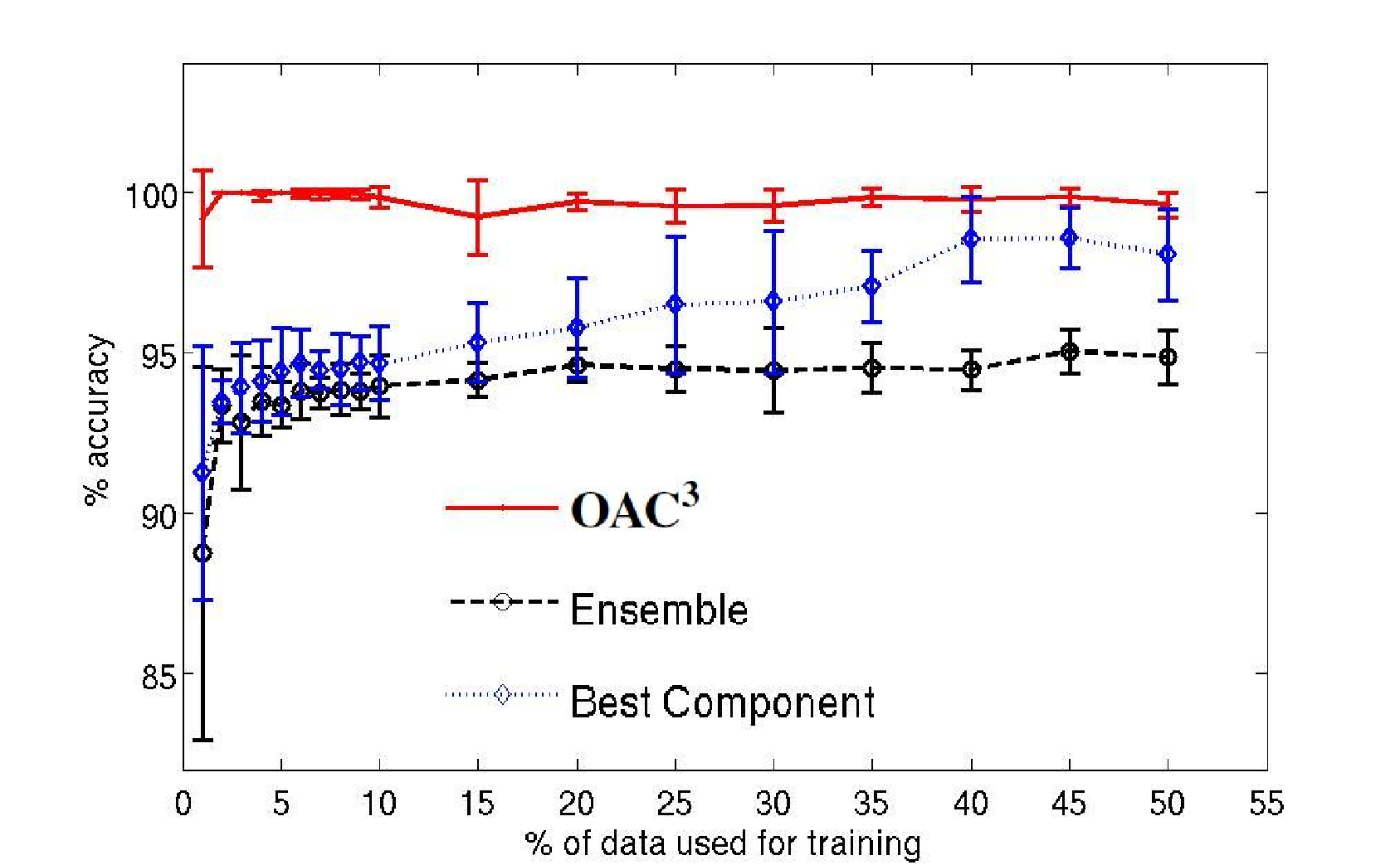
We also evaluate the performance of OAC3 for different proportions (from 1% to 50%) of training data. Fig. 4 summarizes the average accuracies (over 10 trials) achieved by OAC3. The accuracies provided by the classifier ensemble, as well as by its best individual component, are also shown for comparison purposes. The results obtained by OAC3 are consistently better than those achieved by the classifier ensemble. As expected, the curve for OAC3 shows that the less the amount of labeled objects, the greater are the benefits of using the information provided by the cluster ensemble. With 2% of training data, the accuracies observed are 100% in nine trials and 95% in one trial. The mean and standard deviation are 99.5 and 1.59 respectively. This explains why the error bar exceeds 100%.
6.2 Sensitivity Analysis
We perform a sensitivity analysis on the OAC3 parameters by using the same classification datasets employed in [25]. These datasets represent eleven classification tasks from three real-world applications (20 Newsgroups, Cora, and DBLP). There are six datasets (News1 — News6) for 20 Newsgroups and four datasets (Cora1 — Cora4) for Cora. In each task, there is a target set on which the class labels should be predicted. In [25], two supervised models and two unsupervised models were used to obtain (on the target sets) class and cluster labels, respectively. These same class and cluster labels are used as inputs to OAC3. Then, we vary the OAC3 parameters and observe their respective accuracies.
In order to analyze the influence of the parameters and (recall that we set for all i), we consider that the algorithm converges when the relative difference of the objective function in two consecutive iterations is less than . By adopting this criterion, OAC3 usually converges after nine iterations (on average). The algorithm has shown to be robust with respect to . As far as is concerned, for most of the datasets — News1, News3, News4, News6, Cora1, Cora3, Cora4, and DBLP — the classification accuracies achieved from OAC3 are better than those found by the classifier ensemble — no matter the value chosen for . Figure 5 illustrates a typical accuracy surface for different values of and . It is worth mentioning that the accuracy surface tends to keep steady for (i.e., the accuracies do not change significantly). In particular, OAC3 was run for , for which the obtained results are the same as those achieved for for any value of . This same observation holds for all the assessed datasets. The interpretation for such results is that there is a threshold value for that makes the second term of the objective function in (2) dominating — i.e., the information provided by the cluster ensemble is much more important than the information provided by the classifier ensemble.
We observed that for five datasets (News3, News6, Cora1, Cora3, and DBLP) any value of provides the best classification accuracy. Thus, the algorithm can be robust with respect to the choice of its parameters for some datasets. For the datasets News2 and News5, some values yield to accuracy deterioration, thereby suggesting that, depending on the value chosen for , the information provided by the cluster ensemble may hurt — e.g., see Figure 7. Finally, for Cora2, accuracy improvements were not observed, i.e., the accuracies provided by the classifier ensemble were always the best ones. This result suggests that the assumption that classes can be represented by means of clusters does not hold.


As expected, our experiments also show that the number of iterations may influence the performance of the algorithm. In particular, depending on the values chosen for , a high number of iterations may prejudice the obtained accuracies. Considering the best values obtained for in our sensitivity analysis, we observed that, for all datasets, the best accuracies were achieved for less than 10 iterations.
6.3 Comparison with BGCM
As discussed in Section 2, BGCM is the algorithm most closely related to OAC3. We evaluate OAC3 on the same classification datasets employed to assess BGCM [25, 26]. These datasets are those addressed in Section 6.2. In [25], two supervised models (M1 and M2) and two unsupervised models (M3 and M4) were used to obtain (on the target sets) class and cluster labels, respectively. These same labels are used as inputs to OAC3. In doing so, comparisons between OAC3 and BGCM are performed using exactly the same base models, which were trained in the same datasets44 4 For these datasets, comparisons with S3VM [40] have not been performed because the raw data required for learning is not available.. In other words, both OAC3 and BGCM receive the same inputs with respect to the components of the ensembles, from which consolidated classification solutions for the target sets are generated.
For the sake of compactness, the description of the datasets and learning models used in [25] are not reproduced here, and the interested reader is referred to that paper for further details. However, the results for their four base models (M1,…,M4), for BGCM, and for two well-known cluster ensemble approaches — MCLA [41] and HBGF [22] — are reproduced here for comparison purposes. Being cluster ensemble approaches, MCLA and HBGF ignore the class labels, considering that the four base models provide just cluster labels. Therefore, to evaluate classification accuracy obtained by these ensembles, the cluster labels are matched to the classes through an Hungarian method which favors the best possible class predictions. In order to run OAC3, the supervised models (M1 and M2) are fused to obtain class probability estimates for every instance in the target set. Also, the similarity matrix used by OAC3 is calculated by fusing the unsupervised models (M3 and M4).
The parameters of OAC3 have been chosen from the sensitivity analysis performed in Section 6.2. However, for the experiments reported in this section we do not set particular values for each of the (eleven) studied datasets. Instead, we have chosen a set of parameter values that result in good accuracies across related datasets. In particular the following pairs of () are respectively used for the datasets News, Cora, and DBLP: (,); (,); (, ). Such choices will hopefully show that one can get good results by using OAC3 without being (necessarily) picky about its parameter values — thus these results are also complementary to the ones provided in Section 6.2.
Comparison of OAC3 with Other Algorithms — Classification Accuracies (Best Results in Boldface). Method News1 News2 News3 News4 News5 News6 Cora1 Cora2 Cora3 Cora4 DBLP M1 79.67 88.55 85.57 88.26 87.65 88.80 77.45 88.58 86.71 88.41 93.37 M2 77.21 86.11 81.34 86.76 83.58 85.63 77.97 85.94 85.08 88.79 87.66 M3 80.56 87.96 86.58 89.83 87.16 90.20 77.79 88.33 86.46 88.13 93.82 M4 77.70 85.71 81.49 84.67 85.43 85.78 74.76 85.94 78.10 90.16 79.49 MCLA 75.92 81.73 82.53 86.86 82.95 85.46 87.03 83.88 88.92 87.16 89.53 HBGF 81.99 92.44 88.11 91.52 89.91 91.25 78.34 91.11 84.81 89.43 93.57 BGCM 81.28 91.01 86.08 91.25 88.64 90.88 86.87 91.55 89.65 90.90 94.17 OAC3 85.01 93.64 89.64 93.80 91.22 92.59 88.54 90.79 90.60 91.49 94.38
The classification accuracies achieved by the studied methods are summarized in Table 6.3, where one can see that OAC3 shows the best accuracies for all datasets. In order to provide some reassurance about the validity and non-randomness of the obtained results, the outcomes of statistical tests, following the study in [20], are also reported. In brief, multiple algorithms are compared on multiple datasets by using the Friedman test, with a corresponding Nemenyi post-hoc test. The Friedman test is a non-parametric statistic test equivalent to the repeated-measures ANOVA. If the null hypothesis, which states that the algorithms under study have similar performances, is rejected, then the Nemenyi post-hoc test is used for pairwise comparisons between algorithms. The adopted statistical procedure indicates that the null hypothesis of equal accuracies — considering the results obtained by the ensembles — can be rejected at 10% significance level. In pairwise comparisons, significant statistical differences are only observed between OAC3 and the other ensembles, i.e., there is no evidence that the accuracies of MCLA, HBGF, and BGCM are statistically different from one another.
6.4 Comparison with S3VM
We also compare OAC3 to a popular semi-supervised algorithm known as S3VM [40]. This algorithm is essentially a Transductive Linear Support Vector Machine (SVM) which can be viewed as a large scale implementation of the algorithm introduced in [30]. For dealing with unlabeled data, it appends an additional term in the SVM objective function whose role is to drive the classification hyperplane towards low data density regions [40]. The default parameter values have been used for S3VM.
Six datasets are used in our experiments: Half-Moon (see Section 6.1), Circles (which is a synthetic dataset that has two-dimensional instances that form two concentric circles — one for each class), and four datasets from the Library for Support Vector Machines55 5 http://www.csie.ntu.edu.tw/~cjlin/libsvm/ — Pima Indians Diabetes, Heart, German Numer, and Wine. In order to simulate real-world classification problems where there is a very limited amount of labeled instances, small percentages (e.g., 2%) of the instances are randomly selected for training, whereas the remaining instances are used for testing (target set). The amount of instances for training is chosen so that the pooled covariance matrix of the training set is positive definite. This restriction comes from the use of an LDA classifier in the ensemble, and it imposes a lower bound on the number of training instances (7% for Heart and 10% for German Numer). We perform 10 trials for every proportion of instances in the training/target sets. The number of features are 2, 2, 8, 13, 24, 24 for Half-moon, Circles, Pima, Heart, German Numer and Wine respectively.
Comparison of OAC3 with BGCM and S3VM — Average Accuracies (Standard Deviations). Dataset Ensemble Best Component S3VM BGCM OAC3 Half-moon(2%) 784 92.53 93.02 99.61 92.16 99.64 Circles(2%) 1568 60.03 95.74 54.35 78.67 99.61 Pima(2%) 745 68.16 69.93 61.67 69.21 70.31 Heart(7%) 251 77.77 79.22 77.07 82.78 82.85 G. Numer(10%) 900 70.96 70.19 73.00 73.70 74.44 Wine(10%) 900 79.87 80.37 80.73 75.37 83.62
Considering OAC3, the components of the classifier ensemble are chosen as previously described in Section 6.1. Cluster ensembles are generated by means of multiple runs of -means (10 data partitions for the two-dimensional datasets and 50 data partitions for Pima, Heart, German Numer, and Wine).
The parameters of OAC3 ( and ) are optimized for better performance in each dataset using 5-fold cross-validation. The optimal values of for Half-moon, Circles, Pima, Heart, German Numer, and Wine are (0.05,0.1), (0.01,0.1), (0.002,0.1), (0.01,0.2), (0.01,0.1) and (0.01,0.1) respectively. Table 6.4 shows that the accuracies obtained by OAC3 are good and consistently better than those achieved by both the classifier ensemble and its best individual component. In addition, OAC3 shows better accuracies than both S3VM and BGCM — from the adopted statistical procedure [20], OAC3 exhibits significantly better accuracies at a significance level of .
6.5 Transfer Learning
Transfer learning emphasizes the transfer of knowledge across domains, tasks, and distributions that are similar but not the same [39]. We focus on learning scenarios where training and test distributions are different, as they represent (potentially) related but not identical tasks. It is assumed that the training and test domains involve the same class labels. The real-world datasets employed in our experiments are:
a) Text Documents — [35]: From the well-known text collections 20 newsgroup and Reuters-21758, nine cross-domain learning tasks are generated. The two-level hierarchy in both of these datasets is exploited to frame a learning task involving a top category classification problem with training and test data drawn from different sub categories — e.g., to distinguish documents from two top newsgroup categories (rec and talk), the training set is built from “rec.autos”, “rec.motorcycles”, “talk.politics”, and “talk.politics.misc”, and the test set is formed from the sub-categories “rec.sport.baseball”, “rec.sport.hockey”, “talk.politics.mideast”, and “talk.religions.misc”. The Email spam data set, released by ECML/PKDD 2006 discovery challenge, contains a training set of publicly available messages and three sets of email messages from individual users as test sets. The 4000 labeled examples in the training set and the 2500 test examples for each of the three different users differ in the word distribution. A spam filter learned from public sources are used to test transfer capability on each of the users.


b) Botswana — [38]: This is an application of transfer learning to the pixel-level classification of remotely sensed images, which provides a real-life scenario where such learning will be useful — in contrast to the contrived setting of text classification, which is chosen as it has been used previously in [19]. It is relatively easy to acquire an image, but expensive to label each pixel manually, where images typically have about a million pixels and represent inaccessible terrain. Thus typically only part of an image gets labeled. Moreover, when the satellite again flies over the same area, the new image can be quite different due to change of season, thus a classifier induced on the previous image becomes significantly degraded for the new task. These hyperespectral data sets used are from a pixel study area located in the Okavango Delta, Botswana. It has nine different land-cover types consisting of seasonal swamps, occasional swamps, and drier woodlands located in the distal portion of the delta. Data from this region for different months (May, June and July) were obtained by the Hyperion sensor of the NASA EO-1 satellite for the calibration/validation portion of the mission in 2001. Data collected for each month was further segregated into two different areas. While the May scene (Fig. 8) is characterized by the onset of the annual flooding cycle and some newly burned areas, the progression of the flood and the corresponding vegetation responses are seen in the June (Fig. 9) and July (Fig. 10) scenes. The acquired raw data was further processed to produce 145 features. From each area of Botswana, different transfer learning tasks are generated: the classifiers are trained on either May, June or {May June} data and tested on either June or July data.
For text data, we use logistic regression (LR), SVM, and Winnow (WIN) [24] as baseline classifiers. The CLUTO package (http://www.cs.umn.edu/~karypis/cluto) is used for clustering the target data into two clusters. We also compare OAC3 with two transfer learning algorithms from the literature — Transductive Support Vector Machines (TSVM) [29] and the Locally Weighted Ensemble (LWE) [24]. We use Bayesian Logistic Regression http://www.bayesianregression.org/ for running the logistic regression classifier, LIBSVM (http://www.csie.ntu.edu.tw/~cjlin/libsvm/) for SVM, SNoW Learning Architecture http://cogcomp.cs.illinois.edu/page/software_view/1 for Winnow, and SVMlight http://svmlight.joachims.org/ for transductive SVM. The posterior class probabilities from SVM are also obtained using the LIBSVM package with linear kernel. For SNoW, “-S 3 -r 5” is used and the remaining parameters of all the packages are set to their default values. The values of , obtained by 10-fold cross-validation in source domain, are set as and for the transfer learning tasks corresponding to 20 Newsgroup and Spam datasets, respectively. For Reuters-21578, the best values of the parameters are found as , , and for O vs Pe, O vs Pl, and Pe vs Pl, respectively (see Table 6.5). For the hyperspectral data, we use two baseline classifiers: the well-known Naïve Bayes Wrapper (NBW) and the Maximum Likelihood (ML) classifier, which performs well when used with a best bases feature extractor [32]. The target set instances are clustered by -means, varying k from 50 to 70. PCA is also used for reducing the number of features employed by ML. In particular, for the hyperspectral data, cross-validation in the source domain does not result in very good performance. Therefore, we take 5% labeled examples from each of the nine classes of the target data and tune the values of and based on the performance on these examples. The classifiers NBW or ML, however, are not retrained with these examples from the target domain and the accuracies reported in Table 6.5 are on the unlabeled examples only from the target domain.
Classification of 20 Newsgroup, Reuters-21758 and Spam Data. Dataset Mode WIN LR SVM Ensemble TSVM LWE OAC3 20 Newsgroup C vs S 66.61 67.17 67.02 69.58 76.97 77.07 91.25 R vs T 60.43 68.79 63.87 65.98 89.95 87.46 90.11 R vs S 80.11 76.51 71.40 77.39 89.96 87.81 92.90 S vs T 73.93 72.16 71.51 75.11 85.59 81.99 91.83 C vs R 89.00 77.36 81.50 85.18 89.64 91.09 93.75 C vs T 93.41 91.76 93.89 93.48 88.26 98.90 98.70 Reuters-21758 O vs Pe 70.57 66.19 69.25 73.30 76.94 76.77 80.97 O vs Pl 65.10 67.87 69.88 69.21 70.08 67.59 68.91 Pe vs Pl 56.75 56.48 56.20 57.59 59.72 59.90 67.46 Spam spam 1 79.15 56.92 66.28 68.64 76.92 65.60 80.29 spam 2 81.15 59.76 73.15 75.07 84.92 73.36 87.05 spam 3 88.28 64.43 78.71 81.87 90.79 93.79 91.27
The results for text data are reported in Table 6.5. The different learning tasks corresponding to different pairs of categories are listed as “Mode”. OAC3 improves the performance of the classifier ensemble (formed by combining WIN, LR and SVM via output averaging) for all learning tasks, except for O vs Pl, where apparently the training and test distributions are similar. Also, the OAC3 accuracies are better than those achieved by both TSVM and LWE in most of the datasets. Except for WIN, the performances of the base classifiers and clustereres (and hence of OAC3) are quite invariant, thereby resulting in very low standard deviations. The OAC3 accuracies are significantly better than those obtained by both TSVM and LWE (at significance level).
Classification of Hyperspectral Data — Botswana. Dataset Original to Target NBW NBW+OAC3 ML ML+OAC3 PCs Area 1 may to june 70.68 72.61 74.47 81.93 0.0010 0.1 9 may to july 61.85 63.11 58.58 64.32 ) 0.0001 0.2 12 june to july 70.55 72.47 79.71 80.06 0.0012 0.1 127 may+june to july 75.53 80.53 85.78 85.91 0.0008 0.1 123 Area 2 may to june 66.10 71.02 70.22 81.48 0.0070 0.1 9 may to july 61.55 63.74 52.78 64.15 0.0001 0.2 12 june to july 54.89 57.65 75.62 77.04 0.0060 0.1 80 may+june to july 63.79 64.58 77.33 79.59 0.0040 0.1 122
Table 6.5 reports the results for the hyperspectral data. The parameter values () for best performance of OAC3 are also presented alongside. Note that OAC3 provides consistent accuracy improvements for both NBW and ML66 6 Standard deviations of the accuracies from NBW and ML are close to and hence not shown.. In pairwise comparisons, the accuracies provided by OAC3 are significantly better than those obtained by both NBW and ML (at significance level). The column “PCs” indicates the number of principal components used to project the data.
7 Concluding Remarks
We presented a general framework for combining classifiers and clusterers to address semi-supervised and transfer learning problems. The optimization algorithm assumes closed form updates, facilitates parallelization of the same and, therefore, is extremely convenient in handling large scale data – specially with a linear rate of convergence. The proofs for the convergence are quite novel and generalize across a wide variety of Bregman divergences, facilitating one to use proper divergence measure based on the application domain and subsuming many other existing graph based semi-supervised learning algorithms as special cases. The proposed framework has been empirically shown to outperform a variety of algorithms [\citeNPGao_TKDE; \citeNPsind06; \citeNPgafj08] in both semi-supervised and transfer learning problems.
There are few aspects that can be further explored. For example, the impact of the number of classifiers and clusterers in OAC3 deserves further investigation. In addition, a more extensive study across a wide variety of problem domains will reveal the capabilities as well as potential limitations of the framework.
APPENDIX
Appendix A Proofs for Convergence of OAC3
Lemma A.1.
The objective function used in Eq. (4) is separately and jointly strictly convex over . Also, is jointly lower-semi-continuous w.r.t and .
Proof A.2.
- (a)
From the property (a) in Section 4, one can see that is strictly convex w.r.t and separately. From the same property the first term in is strictly convex w.r.t. . The and terms in the objective function can collectively be represented by . This function is jointly convex by property (b) but is not necessarily jointly strictly convex. Suppose and . Then, we have:
Now, it follows that:
(21) which implies that is jointly strictly convex.
- (b)
To prove that is lower-semi-continuous in and jointly, we observe that
(22) The inequality in the step follows from the lower semi continuity of in Section 4 (Property (d)).
The following theorem helps prove that the objective function can be seen as part of a Bregman divergence.
Theorem A.3 ([2]).
A divergence is a Bregman divergence if and only if such that the function satisfies the following conditions:
- (a)
is strictly convex on .
- (b)
is differentiable on .
- (c)
where is the Bregman divergence associated with .
We now introduce a function that is defined as follows:
| (23) |
Note that is different from defined in Eq. (4). The left arguments in the divergences of the first term of are ’s which are assumed to be fixed.
Lemma A.4.
satisfies properties (a) and (b) in Section 4.
Proof A.5.
The proof is direct from the definition of .
Further assume:
with . The vectors , and are each of dimension and formed by concatenating vectors from the set . implies that a new vector is created by repeating for times. For ease of understanding, we also define , . We will assume that whenever a point is mapped to a point , . Similarly, whenever is mapped to . Indeed, both and are bijective mappings.
Example A.6.
To explain the mappings and more clearly, we consider the following example. Let and . Here, – a concatenation of three vectors , and (corrpesponding to three instances) each of which belongs to . Similarly, and . The vector , formed by the transformation on , takes the following form:
Note that this vector has elements each of dimension and hence the dimension of the whole vector is of the form . Similarly,
and,
∎
Now, in light of Theorem A.3, the following corollary is introduced.
Corollary A.7.
If a mapping is defined as:
| (24) |
then is a Bregman divergence.
Proof A.8.
We show that conditions (a), (b) and (c) of Theorem A.3 are satisfied for .
- (a)
Since is a Bregman divergence, such that conditions (a), (b) and (c) are satisfied in corollary A.3 pertaining to this divergence. Note that and . Assume . We now define
(25) Since each of is strictly convex over in Eq. (4) and Eq. (23), is also strictly convex on . Note the emphasis on in the definition of which just ensures that all conditions in Theorem A.3 are satisfied.
- (b)
- (c)
We have ,
The second step follows from the definition of in Eq. (25) and the last step follows from the definition of in Eq. (24). The equality can similarly be proved. Therefore, combining the two results, we have . With a slight abuse of notation, henceforth, we will denote the mapping by with an implicit assumption of the existence of an as described before.
We will see next that we require some definition of for and this explains the definition of in Eq. (24) for the case when .
Lemma A.9.
satisfies properties (a) and (b) in Section 4.
Proof A.10.
- (a)
One can see that is strictly convex separately w.r.t its arguments from its definition in Eq. (24). Since each of and is strictly convex separately w.r.t the arguments and and are bijective mappings, is strictly convex separately w.r.t. and .
- (b)
The joint convexity of also follows directly from its definition and the joint convexity of and .
At this point, we reiterate that defining as in Eq. (24) helps in proving some interesting properties of in a very elegant way. We, in fact, treat as a surrogate for , establish two specific properties of and then show that these properties, by the definition of , translates to the same properties of . The first of them is the 3-Points Property (3-pp) which is introduced in the following definition.
Definition A.11 (3-pp).
Let and be closed convex sets of finite measures. A function is said to satisfy the 3-points property (3-pp) if for a given for which , where and with iff .
Lemma A.12.
satisfies 3-pp.
Proof A.13.
The proof is based on the works of [48]. First, we will show that 3-pp is valid for over . As mentioned earlier, this is where the introduction of becomes useful and elegant. Assume that corresponding to some , corresponding to some and (the fact that the minimizers are just transformations of each other under or follows directly from the separately strict convexity of and ). Therefore,
where, is defined as follows:
| (26) |
Since , , then which implies . Now, by some simple algebra, we can show . By assumption, and hence with achieved iff . If we define then with achieved iff . Note that
| (27) |
Therefore, following 3-pp of over , we can conclude that
| (28) |
which is the 3-pp for .
Lemma A.14.
satisfies properties (c) and (f) mentioned in Section 4.
Proof A.15.
Next, 4-Points Property (4-pp) is introduced.
Definition A.16 (4-pp).
Let and be closed convex sets of finite measures. A function is said to satisfy 4-pp if for a given , where and with iff .
Lemma A.17.
satisfies 4-pp.
Proof A.18.
Assume , , , and . Here, and . From the joint convexity of (established in Lemma A.9) w.r.t both of its arguments we have:
| (29) |
Since minimizes over , we have which, in turn, implies:
Now we have:
Combining the above two equations, we have,
| (30) |
Eq. (30) gets translated for as follows (using definitions of and ):
| (31) |
Hence, satisfies 4-pp.
We now introduce the main theorem that establishes the convergence guarantee of OAC3.
Theorem A.19.
If , , then .
Proof A.20.
The proof here follows the same line of argument as given in [48] and [21]. Since, , we have, . By the 3-pp, . Then,
This implies that the sequence is non-increasing and non-negative. Let, . From 4-pp and 3-pp, we can derive the following two inequalities:
| (32) | |||||
| (33) |
Combining the above two inequalities, we get:
| (34) |
which is the 5-points property (5-pp) of . From (34), the sequence is non-increasing and non-negative. Therefore, it must have a limit (from the Monotone Convergence Theorem) and consequently the left hand side of (34) approaches 0 as . Hence, (by the Pinching Theorem).
Finally, we must show that and themselves converge. From the boundedness of (established in Lemma A.14), it follows that is bounded. Therefore, it has a convergent subsequence – the limit of which can be denoted by (by the Bolzano-Weierstrass Theorem). Similarly, it can be shown that the subsequence also converges to some limit. Let that limit be denoted by . By the lower-semi-continuity of (established in Lemma A.1), we have:
| (35) |
We denote and . Therefore, from the joint strict convexity of , we should have and .
To prove the convergence of the entire sequence, we apply the same logic as above with replaced by . Then the sequence is bounded and non-increasing and by using Lemma A.14, we conclude that it has a convergent subsequence that goes to as . This, from Monotone Convergence Theorem, implies that and again using Lemma A.14, we can conclude that . Since is also bounded, it should have a convergent subsequence (by the Bolzano-Weierstrass Theorem). We denote this limit by . Again, by the lower-semi-continuity of , we have:
| (36) |
Hence, and .
There is another interesting aspect of that was discovered in [42] for a slightly different objective function with KL divergence used as a loss function. The same property also holds for if the loss function is constructed from the assumed family of Bregman divergences. This property is concerned with the equality of solutions of and and explores under what conditions these two objectives become equal. To establish the theorem that explores this condition, the following lemmata are essential.
Lemma A.21.
If then .
Proof A.22.
Lemma A.23.
.
Proof A.24.
The last step is due to the fact that the unconstrained minima is never larger than the constrained minima.
Lemma A.25.
Given any , , such that , , and (i.e. not all components are equal) then there exists a finite such that .
Proof A.26.
The theorem that formulates the conditions for equality of solutions of and is given below:
Theorem A.27 (Equality of Solutions of and ).
Let and for an arbitrary . Then there exists a finite such that at convergence of OAC3, we have . Further, if , then
and if , then .
Proof A.28.
If , then from the strict convexity of both and , . Also, since for any , , whenever , then . Also, if , then from Lemma A.25, if
then it is guaranteed that .
Appendix B Proof for Analysis of Rate of Convergence
Lemma B.1.
is positive definite over the domain of under the assumption when KL or generalized I divergence is used as a Bregman divergence.
Proof B.2.
Assume . Now,
| (37) | |||||
Therefore, if , is positive definite over the domain of .
We are grateful to Luiz F. S. Coletta for running the experiments described in Section 6.2. We also thank Ambuj Tewari and Ali Jalali for pointing us to relevant literarure for analyzing the rate of convergence of the optimization framework.
References
- Acharya et al. (2011) Acharya, A., Hruschka, E. R., Ghosh, J., and Acharyya, S. 2011. C3E: A Framework for Combining Ensembles of Classifiers and Clusterers. In MCS. 269–278.
- Banerjee et al. (2005) Banerjee, A., Merugu, S., Dhillon, I. S., and Ghosh, J. 2005. Clustering with Bregman Divergences. JMLR 6, 1705–1749.
- Belkin et al. (2005) Belkin, M., Niyogi, P., and Sindhwani, V. 2005. On Manifold Regularization. In AISTAT.
- Bengio et al. (2006) Bengio, Y., Delalleau, O., and Le Roux, N. 2006. Label Propagation and Quadratic Criterion. In Semi-Supervised Learning, O. Chapelle, B. Schölkopf, and A. Zien, Eds. MIT Press, 193–216.
- Bezdek and Hathaway (2002) Bezdek, J. and Hathaway, R. 2002. Some notes on alternating optimization. In Advances in Soft Computing — AFSS 2002, N. Pal and M. Sugeno, Eds. Lecture Notes in Computer Science Series, vol. 2275. Springer Berlin / Heidelberg, 187–195.
- Bezdek and Hathaway (2003) Bezdek, J. C. and Hathaway, R. J. 2003. Convergence of alternating optimization. Neural, Parallel Sci. Comput. 11, 4, 351–368.
- Blum (1998) Blum, A. 1998. On-line algorithms in machine learning. In Online Algorithms: The State of the Art, Fiat and Woeginger, Eds. LNCS Vol.1442, Springer.
- Bollacker and Ghosh (2000) Bollacker, K. D. and Ghosh, J. 2000. Knowledge transfer mechanisms for characterizing image datasets. In Soft Computing and Image Processing. Physica-Verlag, Heidelberg.
- Boyd et al. (2011) Boyd, S., Parikh, N., Chu, E., Peleato, B., and Eckstein, J. 2011. Distributed optimization and statistical learning via the alternating direction method of multipliers. Tech Report.
- Bregman (1967) Bregman, L. M. 1967. The relaxation method of finding the common point of convex sets and its application to the solution of problems in convex programming. USSR Computational Mathematics and Mathematical Physics 7, 3, 200 – 217.
- Cai et al. (2009) Cai, W., Chen, S., and Zhang, D. 2009. A simultaneous learning framework for clustering and classification. Pattern Recognition 42, 1248–1259.
- Caruana (1997) Caruana, R. 1997. Multitask learning. Mach. Learn. 28, 41–75.
- Censor and Zenios (1997) Censor, Y. A. and Zenios, S. A. 1997. Parallel Optimization: Theory, Algorithms and Applications. Oxford University Press.
- Chapelle et al. (2006) Chapelle, O., Schölkopf, B., and Zien, A. 2006. Semi-Supervised Learning. MIT Press.
- Chen et al. (2009) Chen, S., Guo, G., and Chen, L. 2009. Semi-supervised classification based on clustering ensembles. In Proc. of AICI ’09. Springer-Verlag, 629–638.
- Cheney and Goldstein (1959) Cheney, W. and Goldstein, A. A. 1959. Proximity maps for convex sets. Proceedings of the American Mathematical Society 10, 3, pp. 448–450.
- Corduneanu and Jaakkola (2003) Corduneanu, A. and Jaakkola, T. 2003. On information regularization. In UAI. 151–158.
- Csiszár and Tusnády (1984) Csiszár, I. and Tusnády, G. 1984. Information geometry and alternating minimization procedures. Statistics aand Decisions, Supplement Issue 1, 1, 205–237.
- Dai et al. (2007) Dai, W., Xue, G., Yang, Q., and Yu, Y. 2007. Co-clustering based classification for out-of-domain documents. In Proc. of KDD. New York, NY, USA, 210–219.
- Demsar (2006) Demsar, J. 2006. Statistical comparison of classifiers over multiple data sets. Journal of Machine Learning Research 7, 7, 1–30.
- Eggermont and LaRiccia (1998) Eggermont, P. and LaRiccia, V. 1998. On em-like algorithms for minimum distance estimation. Unpublished manuscript, University of Delaware.
- Fern and Brodley (2004) Fern, X. and Brodley, C. 2004. Solving cluster ensemble problems by bipartite graph partitioning. In Proc. of ICML. 281–288.
- Forestier et al. (2010) Forestier, G., Gançarski, P., and Wemmert, C. 2010. Collaborative clustering with background knowledge. Data Knowl. Eng. 69, 211–228.
- Gao et al. (2008) Gao, J., Fan, W., Jiang, J., and Han, J. 2008. Knowledge transfer via multiple model local structure mapping. In Proc. of KDD. 283–291.
- Gao et al. (2009) Gao, J., Liang, F., Fan, W., Sun, Y., and Han, J. 2009. Graph-based consensus maximization among multiple supervised and unsupervised models. In Proc. of NIPS. 1–9.
- Gao et al. (2011) Gao, J., Liang, F., Fan, W., Sun, Y., and Han, J. 2011. A graph-based consensus maximization approach for combining multiple supervised and unsupervised models. IEEE Transactions on Knowledge and Data Engineering accepted for publication.
- Ghosh and Acharya (2011) Ghosh, J. and Acharya, A. 2011. Cluster ensembles. WIREs Data Mining and Knowledge Discovery 1, 1–12.
- Gunawardana and Byrne (2005) Gunawardana, A. and Byrne, W. 2005. Convergence theorems for generalized alternating minimization procedures. J. Mach. Learn. Res. 6, 2049–2073.
- Joachims (1999a) Joachims, T. 1999a. Making large-scale SVM learning practical. In Advances in Kernel Methods: Support Vector Learning, C. B. B. Scholkopf and A. Smola, Eds. MIT Press, 169–184.
- Joachims (1999b) Joachims, T. 1999b. Transductive inference for text classification using support vector machines. In Proc. of ICML. 200–209.
- Joachims (2003) Joachims, T. 2003. Transductive learning via spectral graph partitioning. In Proceedings of the Twentieth International Conference on Machine Learning (ICML-2003).
- Kumar et al. (2001) Kumar, S., Ghosh, J., and Crawford, M. M. 2001. Best-bases feature extraction algorithms for classification of hyperspectral data. IEEE TGRS 39, 7, 1368–79.
- Kuncheva (2004) Kuncheva, L. I. 2004. Combining Pattern Classifiers: Methods and Algorithms. Wiley, Hoboken, NJ.
- Oza and Tumer (2008) Oza, N. C. and Tumer, K. 2008. Classifier ensembles: Select real-world applications. Inf. Fusion 9, 4–20.
- Pan and Yang (2010) Pan, S. J. and Yang, Q. 2010. A survey on transfer learning. IEEE TKDE 22, 1345–1359.
- Polikar (2007) Polikar, R. 2007. Bootstrap-inspired techniques in computational intelligence. IEEE SIGNAL PROCESSING MAGAZINE.
- Punera and Ghosh (2008) Punera, K. and Ghosh, J. 2008. Consensus based ensembles of soft clusterings. In Applied Artificial Intelligence. Vol. 22. 109–117.
- Rajan et al. (2006) Rajan, S., Ghosh, J., and Crawford, M. M. 2006. Exploiting class hierarchies for knowledge transfer in hyperspectral data. IEEE TGRS 44, 11, 3408–3417.
- Silver and Bennett (2008) Silver, D. L. and Bennett, K. P. 2008. Guest editor’s introduction: special issue on inductive transfer learning. Mach. Learn. 73, 215–220.
- Sindhwani and Keerthi (2006) Sindhwani, V. and Keerthi, S. S. 2006. Large scale semi-supervised linear SVMs. In Proc. of the 29th Annual International ACM SIGIR Conf. on Research and Development in Information Retrieval. NY, USA, 477–484.
- Strehl and Ghosh (2002) Strehl, A. and Ghosh, J. 2002. Cluster ensembles – a knowledge reuse framework for combining multiple partitions. JMLR 3, 583–617.
- Subramanya and Bilmes (2011) Subramanya, A. and Bilmes, J. 2011. Semi-supervised learning with measure propagation. Journal of Machine Learning. Research 12, 3311–3370.
- Subramanya and Bilmes (2009) Subramanya, A. and Bilmes, J. A. 2009. Entropic graph regularization in non-parametric semi-supervised classification. In Proc. of NIPS. Vancouver, Canada.
- Thrun and Pratt (1997) Thrun, S. and Pratt, L. 1997. Learning To Learn. Kluwer Academic, Norwell, MA.
- Tsuda (2005) Tsuda, K. 2005. Propagating distributions on a hypergraph by dual information regularization. In Proceedings of the 22nd international conference on Machine learning. ICML ’05. ACM, New York, NY, USA, 920–927.
- Tumer and Ghosh (1996) Tumer, K. and Ghosh, J. 1996. Analysis of decision boundaries in linearly combined neural classifiers. Pattern Recognition 29, 2, 341–348.
- Wang et al. (2011) Wang, H., Shan, H., and Banerjee, A. 2011. Bayesian cluster ensembles. Statistical Analysis and Data Mining 1, 1–17.
- Wang and Schuurmans (2003a) Wang, S. and Schuurmans, D. 2003a. Learning continuous latent variable models with bregman divergences. 2842, 190–204.
- Wang and Schuurmans (2003b) Wang, S. and Schuurmans, D. 2003b. Learning latent variable models with Bregman divergences. In IEEE International Symposium on Information Theory.
- Wu (1982) Wu, C. F. J. 1982. On the convergence properties of the EM algorithm. Annals of Statistics.
- Zangwill (1969) Zangwill, W. 1969. Nonlinear Programming: a Unified Approach. Prentice-Hall International Series in Management, Englewood Cliffs: N.J.
- Zhang et al. (2006) Zhang, T., Popescul, A., and Dom, B. 2006. Linear prediction models with graph regularization for web-page categorization. In Proc. of the 12th ACM SIGKDD. ACM, New York, NY, USA, 821–826.
- Zhu (2005) Zhu, X. 2005. Semi-supervised learning with graphs. Ph.D. thesis, Pittsburgh, PA, USA. Chair-Lafferty, John and Chair-Rosenfeld, Ronald.
- Zhu and Ghahramani (2002) Zhu, X. and Ghahramani, Z. 2002. Learning from labeled and unlabeled data with label propagation. Tech. rep., Carnegie Mellon University.
- Zhu and Goldberg (2009) Zhu, X. and Goldberg, A. B. 2009. Introduction to Semi-Supervised Learning. Morgan & Claypool Publishers.
April 2012April 2012