Finite-time Convergent Gossiping

Gossip protocols have become canonical solutions in modern distributed computer systems for their simplicity and scalability [1, 2, 3]. For a network of nodes without central coordinator, gossip protocols provide an information spread mechanism in which nodes communicate pairwise along with some deterministic or randomized pair-selection algorithm [4]. Formally, a gossip protocol consists of two parts [5]: an underlying algorithm determining pairwise node interactions for point-to-point communication, and an interaction rule built on top of the algorithm determining the information for exchange and the way nodes update their internal states. Gossip-based protocols have been adopted to provide distributed solutions in the areas of optimization, control, signal processing, and machine learning [6, 7, 8, 9], and recently have even been generalized to quantum information processing leading to the development of quantum gossiping algorithms [10, 11].

The convergence speed of the underlying gossip algorithm associated with a given gossip protocol, serves naturally as the primary index to the performance of the protocol. In literature, characterizations of gossip algorithm convergence focus on two basic convergence-rate metrics: information dissemination and aggregation times. The dissemination time concerns the minimum number of steps it takes for a message starting from one node to spread across the whole network with a probability no smaller than a given level [12]. The aggregation time concerns the minimum number of steps it takes for nodes in the network to compute a generic function (e.g., initial values’ average) to a given accuracy with a given probability [13]. These two metrics are essentially asymptotic rates of the probability decrease for the hitting/mixing times being smaller than the current time slot, along a Markovian process defined by the random gossiping. Various efforts have been made on bounding and optimizing these two convergence metrics [14, 15, 12, 13, 16, 17, 18, 19, 20, 21, 22], where it has been shown that they are determined by the pair selection mechanism and the structure of the underlying network.

Finite-time convergence then naturally serves as an intriguing limit in studying the convergence properties of gossip algorithms. In a more general domain, the possibilities and impossibilities of reaching finite-time convergence for discrete-time consensus algorithms, represented by products of stochastic matrices, have been systematically investigated in [23, 24, 25, 26]. These distributed algorithms have a finite computational cost, and surprisingly, certain distributed algorithms converging in finite time can be faster than any possible centralized algorithm [25]. In this paper, we restrict our attention to deterministic gossip algorithms and study their finite-time convergence, which will, generally speaking, provide faster information spreading than any asymptotically convergent gossip protocols.

Consider a network with node set $\mathrm{V}=\{1,\dots,n\}$. Time is slotted and the value node $i$ holds at time $k$ is denoted as $x_{i}(k)\in\mathbb{R}$ for $k\geq 0$. The global network state is then given by $x(k)=(x_{1}(k)\dots x_{n}(k))^{T}$. A symmetric deterministic gossip algorithm [13, 16] is defined by a sequence of node pairs $(i_{k},j_{k})$ for $k=0,1,\dots$ and a node state update rule

Note that the two selected nodes update their state to the average of the values they held prior to the interaction, while the states of all other nodes remain unchanged.

Introduce

where $I_{n}$ is the $n$ by $n$ identity matrix, and $e_{m}=(0\dots 0\ 1\ 0\dots 0)^{T}$ is the $n\times 1$ unit vector whose $m$’th component is $1$. We can write the class of all deterministic gossip algorithms as

Algorithm (2) is called an asymmetric gossip algorithm if we replace $\mathscr{M}_{n}$ with [28]

In this case, it is allowed that only one of the interacting nodes updates its state.

Let $\mathbf{1}$ denote the all-one column vector with proper dimension. We now consider the following definition of finite-time convergence.

Note that global finite-time convergence is equivalent to ${\rm rank}(P_{T-1}\cdots P_{0})=1$ for some $T\geq 1$. Let $\|\cdot\|_{1}$ be the matrix norm defined by $\|A\|_{1}=\sum_{i=1}^{m}\sum_{j=1}^{n}\big|[A]_{ij}\big|$ for any $A\in\mathbb{R}^{m\times n}$ with $\big|\cdot\big|$ denoting the absolute value. We use the following definition of computational complexity of finite-time gossip algorithms:

In this paper, we obtain the following two results for symmetric and asymmetric gossip algorithms, respectively.

The two theorems are obtained by first establishing a lower bound on the number of node updates required for reaching finite-time consensus, and then explicitly constructing gossip algorithms that converge in a finite number of steps equal to the lower bound. Although we allow every node to interact with every other node (i.e., we do not impose any restricted network structure on the allowed interactions), the fastest convergent algorithms only use a subset of the edges. In fact, we prove that for $n=4$, finite-time convergent symmetric algorithms are essentially unique. If the sequence of node pairs $(i_{k},j_{k}),k=0,1,\dots$ is defined by an independent random process, the above deterministic finite-time convergent gossiping implies fundamental robustness in the presence of repulsive links in light of the the Borel-Cantelli Lemma [29]. Moreover, the deterministic finite-time convergent results established in the current paper can be used to derive almost sure finite-time convergence results under random gossiping models [30]. Theorem 1 and 2 were briefly reported in [31].

We apply the obtained results to recent studies on quantum gossip algorithms. In [10, 11], a gossiping algorithm was introduced to quantum systems in the aim of symmetrizing the information contained in each qubit of an $n$-qubit quantum network. Accurate operations to large-scale quantum systems play a fundamental role in quantum information processing due to the exponentially growing system dimension and the fragility of state preservation. We reveal that any $n$-qubit quantum gossiping algorithm is equivalent to a number of decoupled symmetric gossip algorithms, with numbers of nodes ranging from $\binom{n}{0}$ to $\binom{n}{n}$. Therefore finite-time convergence can never be achieved for any nontrivial quantum gossiping since $\binom{n}{0},\binom{n}{1},\dots,\binom{n}{n}$ cannot all be equal to some of power of two as long as $n\neq 2$. This result is summarized as follows.

In Theorem 3, by saying global finite-time convergence to full symmetrization, we mean that the steady symmetric state consensus (cf., [10]) is reached in some finite steps for all initial values as proper quantum states represented by density operators. Theorem 3 indicates some strong impossibility of finite-time convergence to symmetric states for quantum gossiping algorithms. However, it should be emphasized that, the reduced states of the qubits essentially follow the same dynamics as the classical symmetric gossip algorithms, and therefore we can apply Theorem 1 to conclude that these reduced states will converge to an agreement in finite time if and only if the number of qubits is some power of two. This point will be detailed in Section 4.

The authors of [10, 11] have shown some conceptual consistency between the classical and quantum gossip algorithms from a group-theoretic perspective, and it was shown in [10] that the asymptotic convergence of quantum gossip algorithms follows the same contraction-mapping analysis as its classical analogue [16]. For quantum gossip algorithms, the distinction between their finite-time convergence in reduced states and their impossibility of reaching finite-time convergence in symmetric states arises directly from the quantum specificities of the network.

Section 2 focuses on the analysis of symmetric gossiping. An all-or-nothing lemma is given for general averaging algorithms for the proof of the necessity statement of Theorem 1. We also discuss the number of algorithms reaching finite-time convergence. Section 3 then turns to asymmetric gossip algorithms. We establish a combinatorial lemma, by which we show the necessary number of node updates. We then construct an asymmetric algorithm which converges with the given number of node updates. Section 4 discusses the application of the obtained results to quantum gossip algorithms and proves Theorem 3 after a brief introductory to quantum states and quantum gossip algorithms. Finally some concluding remarks are given in Section 5.

All vectors are column vectors and denoted by lower case letters. Matrices are denoted with upper case letters. The sets of integers, real numbers, and complex numbers are denoted as and $\mathbb{Z}$, $\mathbb{R}$, and $\mathbb{C}$, respectively. Also, $\mathbb{Z}^{\geq 0}$ and $\mathbb{Z}^{+}$ denote the sets of positive and nonnegative integers, respectively. A finite square matrix $M\in\mathbb{R}^{n\times n}$ is called stochastic if $[M]_{ij}\geq 0$ for all $i,j$ and $\sum_{j}[M]_{ij}=1$ for all $i$ [27]. A stochastic matrix $M$ is called doubly stochastic if $M^{T}$ is also stochastic. Denote $\mathsf{S}\doteq\big\{W\in\mathbb{R}^{n\times n}:\ W\mbox{ is a stochastic matrix}\big\}$ as the set of $n\times n$ stochastic matrices. Given a matrix $M\in\mathbb{C}^{m\times n}$, the vectorization of $M$, denoted by ${\rm\bf vec}(M)$, is the $mn\times 1$ column vector $([M]_{11},\dots,[M]_{m1},\dots,[M]_{1n},\dots,[M]_{mn})^{T}$. For all matrices $A,B,C$ with $ABC$ well defined, it holds that ${\rm\bf vec}(ABC)=(C^{T}\otimes A){\rm\bf vec}(B)$ , where $\otimes$ is the Kronecker product [37].

We first prove the existence of the critical number of nodes by a contradiction argument. Suppose that $n=2^{n_{1}}n_{2}$ with $n_{1}\geq 0$ and $n_{2}\geq 3$ an odd integer, and suppose that there exists a finite integer $k_{\ast}$ and $P_{0},\dots,P_{k_{\ast}}\in\mathscr{M}_{n}$ so that (2) converges globally in $k_{\ast}+1$ steps. This means that there exists a constant $c\in\mathbb{R}$ such that $x_{i}(k_{\ast}+1)=c$ for all $i\in V$. Consider the initial value $x_{1}(0)=x_{2}(0)=\dots=x_{2^{n_{1}}}(0)=0$ and $x_{2^{n_{1}}+1}(0)=\dots=\dots,x_{n}(0)=2^{k_{\ast}+1}$. Since each element in $\mathscr{M}_{n}$ is symmetric and doubly stochastic, the initial average is preserved at every iteration. Thus,

On the other hand, it is not hard to see that $c$ is an integer for the given initial value, since pairwise averaging takes place $k_{\ast}+1$ times. Consequently, we have $c=r_{2}2^{r_{1}}$ with $0\leq r_{1}\leq k_{\ast}+1$ an integer and $r_{2}\geq 1$ an odd integer. Therefore, we conclude that

which implies that

Since the left-hand side of Eq. (3) is an even number while the right-hand side is odd, we have reached a contradiction. Therefore, when $n$ is not a power of two, Algorithm (2) with symmetric updates cannot achieve global finite-time convergence no matter how $P_{0},\dots,P_{k_{\ast}}$ are chosen.

Recall that $\mathsf{S}$ denotes the set of $n\times n$ stochastic matrices. Algorithm (2) is a special case of distributed averaging algorithms defined by products of stochastic matrices [42, 43]:

Let $\mathsf{S}_{0}\subseteq\mathsf{S}$ be a subset of $\mathsf{S}$. We define

Let ${\mu}(\cdot)$ represent the standard Lebesgue measure on $\mathbb{R}^{n}$. We have the following lemma for the finite-time convergence of averaging algorithm (4).

Noticing that $\mathscr{M}_{n}$ is a finite set and utilizing Lemma 1, Claim (ii) of Theorem 1 follows immediately. The proof of Lemma 1 is given in Appendix A.

Now let $n=2^{m}$ for some integer $m\geq 0$. For any given symmetric gossip algorithm $\{P_{k}\}_{0}^{\infty}$, we define

and let $[\Psi_{h}]_{ij}$ denote the $ij$-entry of $\Psi_{h}$. We call node $i$ active in matrix $P_{k}$ if the $ii$-entry of $P_{k}$ equals $1/2$. Define

Then, the following claim holds.

This claim can be easily proved using a recursive argument.

We introduce

Invoking the claim we clearly see that $s_{i}(K)\geq m$. That is to say, when global finite-time convergence is achieved, each node must have been active for at least $m$ times. Since only two nodes are updated in each iteration $k$, $K$ is at least $mn/2$. It is then straightforward to see that $\mathbf{C}_{n}=mn$.

Let $n=2^{m}$. We now present a symmetric gossip algorithm that converges globally in $nm=n\log_{2}n$ node updates. Such an algorithm can be easily constructed recursively: Let the $n$ nodes be divided into two subsets with an equal number ($n/2$) of nodes and suppose agreement has been achieved via symmetric gossiping, respectively, for each subset of nodes. Then obviously finite-time agreement can be realized for the $n$ nodes after pairwise matching the nodes in the two subsets and running a symmetric gossiping update among each of the pairs.

We remark that essentially the same algorithm has been proposed implicitly in Example 2.4 of [35]. Moreover, such a recursive construction is one of the key components of the classical Cooley-Tukey algorithm [32] for fast Fourier transform (FFT), and in fact the symmetric gossiping algorithm that we present below is even a special case of Cooley-Tukey arrangement for inverse discrete Fourier transform (IDFT), where the average value corresponds to zero-frequency coefficient [33]. The Cooley-Tukey algorithm however also made use of the periodic nature of the exponential multipliers in FFT so the matching between two subsets of $n/2$ nodes needs to be carefully selected, which is not required for reaching a simple finite-time agreement in our case. Nonetheless, for the completion of the paper we would like to make a full exposure to this algorithm.

Introduce the notation $M_{ij}:=I_{n}-{(e_{i}-e_{j})(e_{i}-e_{j})^{T}}/{2}$ and associate each node $i\in\mathrm{V}$ with the binary representation

of the value $i-1$. We denote the $k$’th digit of the binary representation of $i-1$ as $[D_{k}]^{i}$. We present the following algorithm as a matrix selection process in $\mathscr{M}_{n}$:

The algorithm proceeds in $m$ stages. In each stage $s$, a set $\mathsf{P}_{s}$ of all selection matrices $M_{ij}$ involving the node pairs $\{i,j\}$, with $[D_{s}]^{i}\neq[D_{s}]^{j}$ and $[D_{l}]^{i}=[D_{l}]^{j},l\neq s$, is formed. We apply the matrices for symmetric gossiping following the order of subsets $\mathsf{P}_{1},\dots,\mathsf{P}_{m}$, where matrices in the same $\mathsf{P}_{s}$, $s=1,\dots,m$ can be put in arbitrary order since they commute with each other (we have used $\mathsf{P}_{s}[t]$ to denote the $t$’th element in $\mathsf{P}_{s}$). It is easy to verify that after all matrices in $\mathsf{P}_{s}$ have been applied there are at most $2^{m-s}$ different values left in the network for $s=1,\dots,m$. Thus, convergence is reached after $mn=n\log_{2}n$ node updates.

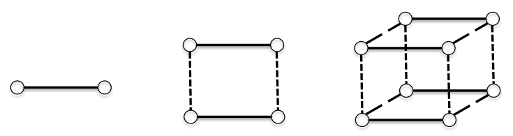
Although we don’t intend to discuss how the structure of the graph influences the existence and complexity of finite-time convergent gossiping, the proposed Algorithm 1 certainly only makes use of a fraction of edges, which naturally induces a graphical structure. Indeed, the construction of Algorithm 1 is inspired by “hypercubes”, whose precise definitions are given as follows:

In Algorithm 1, the selected edges are exactly those who form a $\log_{2}n$-dimensional Hypercube with $n$ nodes. They are selected in the order that arises naturally from the definition of the Cartesian product (see Figure 1).

We have shown that Algorithm 1 gives a fastest possible convergence. It is intriguing to ask if this algorithm is the only one that achieves finite-time consensus, or if there are (possibly many) other equally fast symmetric gossip algorithms. This turns out to be a difficult question to answer. We can, however, establish the following result indicating that for $n=4$ nodes, all finite-time convergent symmetric gossip algorithms can be reduced to an essentially unique form.

The proof of Proposition 1 is given in Appendix B.

In this subsection, we first establish the least number of node updates for finite-time convergence via asymmetric gossiping. Let $n=2^{m}+r$ with $0\leq r<2^{m}$. The following combinatorial lemma decomposes $1$ into $n$ suitable fractions, whose proof can be found in Appendix C.

Given any algorithm $\{P_{k}\}_{0}^{\infty}$, we continue to use the notations by which we analyze the symmetric case. Recall that

Just like the symmetric case, we define $s_{i}(h)$ as the number of $P_{k}$’s such that node $i$ is active in $P_{k},k=1,\dots,h-1$ and assume the algorithm converges within $K$ steps, i.e., all rows of $\Psi_{K}$ are the same.

The following lemma follows from a simply recursive argument.

Since all rows of $\Psi_{K}$ are the same, it follows that $\sum_{i=1}^{n}[\Psi_{K}]_{ii}=\sum_{i=1}^{n}[\Psi_{K}]_{1i}=1$. That is to say, $f_{\ast}:=([\Psi_{K}]_{11}\ [\Psi_{K}]_{22}\ ...\ [\Psi_{K}]_{nn})$ is an element of the set $\mathbb{F}$ defined in Lemma 2. Furthermore, by Lemma 3. (ii), $[\Psi_{K}]_{ii}\geq{1}/{2^{s_{i}(K)}}$. According to the definition of $\chi_{i}$ in Lemma 2, $s_{i}(K)\geq\chi_{i}(f_{\ast})$. Therefore, $\sum_{i=1}^{n}s_{i}(K)\geq\sum_{i=1}^{n}\chi_{i}(f_{\ast})\geq mn+2r$ based on Lemma 2, i.e., the number of node updates is at least $nm+2r$ for reaching convergence.

We now construct an algorithm that when node states converge to the same value, only $nm+2r$ node updates have been taken. Denote $M^{*}_{ij}:=I_{n}-{e_{i}(e_{i}-e_{j})^{T}}/{2}$.

Again, we relabel the nodes in a binary system. We use the binary number

to mark node $i$ if $B_{1}\dots B_{m+1}=i-1$ as a binary number. We denote the $k$’th digit of $i-1$ in this binary system as $[D_{k}]^{i}$ for $k=1,\dots,m+1$ and $i=1,\dots,n$. We present the following algorithm.

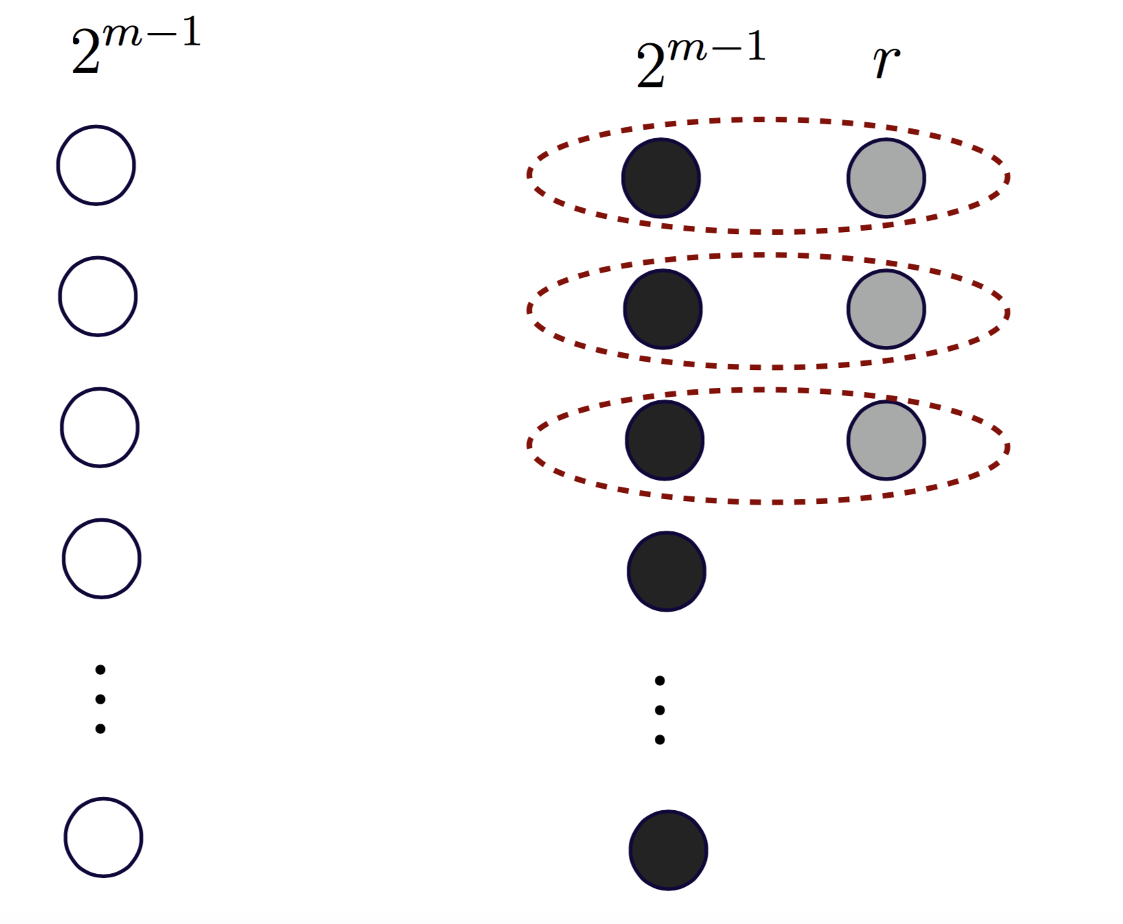
Algorithm 2 selects a sequential subsets of matrices in $\mathscr{M}^{\natural}$, indexed by $\mathsf{P}_{1},\ \mathsf{P}_{2}^{\sharp},\ \mathsf{P}_{2},\ \mathsf{P}_{3}^{\sharp},\ \mathsf{P}_{3}$, $\dots,\ \mathsf{P}_{m+1}^{\sharp},\ \mathsf{P}_{m+1}$. Matrices in the same subset can be put in arbitrary orders since they commute with each other. Matrices in $\mathsf{P}_{s},s=1,\dots,m+1$ are symmetric, while matrices in $\mathsf{P}_{s}^{\sharp},s=2,\dots,m+1$ are asymmetric. It is straightforward to verify that after all matrices in $\mathsf{P}_{s}$ have been applied, at most $2^{m-s+1}$ different value remain in the network. The number of node updates in Algorithm 2 can be easily calculated to be exactly $mn+2r$.

An illustration of Algorithm 2 for three nodes is shown in Figure 2. Note that after the first step Node $1$ and Node $2$ hold the same value (say, $a$) and Node $3$ holds a maybe different one (say, $b$), while the three nodes eventually agree on $({a}+{b})/{2}$ after the next two steps. Therefore, after the first step Nodes $1$ and $2$ can be viewed as have been tied together as one node which carries out a symmetric update with Node $3$.

Algorithm 2 is constructed based on the above intuition for three nodes. For $n=2^{m}+r$ nodes with distinct values, matrices in $\mathsf{P}_{1}$ carry out $r$ pairs of symmetric averaging and leave only $2^{m}$ different values. In this way $2r$ nodes are grouped into $r$ virtual nodes and then the $2^{m}$ different values reach finite-time convergence as in Algorithm 1 with the help of asymmetric updates (cf., Figure 3).

Information processing over quantum mechanical systems is the foundation of quantum communication and quantum computation, where fundamental challenges arise from quantum mechanics [36]. In this subsection, we give a brief introduction to quantum system states and we refer the readers to [36] for a comprehensive treatment.

Introduce a notion of time indexed by $k=0,1,\dots$, and let $\rho(k)$ denote the density operator of the considered $n$-qubit network at time $k$. The quantum gossip algorithm introduced in [10, 11] can then be written as

where $S(k)\in\mathfrak{U},\ k=0,1,\dots$ and $S^{{\dagger}}$ is the conjugate transpose of the operator $S$.

It has been shown in [10, 11] that under quite general (randomized or deterministic) conditions on the swapping sequence, Algorithm (5) converges asymptotically to the symmetric state

where $\mathbf{P}$ is the permutation group over $\mathrm{V}$, and $U_{\pi}$ is the unitary operator over $\mathcal{H}^{\otimes n}$ defined by

for any $\pi\in\mathbf{P}$.

In the remainder of this section, we establish the proof of Theorem 3. We first establish a relationship between the quantum gossip algorithm and its classical analogue. Then the conclusion follows directly from the critical node number condition and the “all-or-nothing” lemma that we have derived earlier.

For ease of presentation we identify the linear operators $\rho$, $U_{ij}$, and $U_{\pi}$ as their matrix representations in $\mathbb{C}^{2^{n}\times 2^{n}}$ under the standard computational basis of $\mathcal{H}^{\otimes n}$ in the rest of discussions. Under vectorization, Algorithm (5) can be rewritten into the following vector form:

where ${S(k)}\in\mathfrak{U},\ k=0,1,\dots$ and $I$ is the $4^{n}$ by $4^{n}$ identity matrix.

Associated with any swapping operator $U_{ij}\in\mathfrak{U}$, we naturally define a quantum graph, $\mathrm{G}=(\mathrm{V},\mathrm{E})$, where $\mathrm{E}:=\big\{\{i,j\}\big\}$ is the quantum edge set containing only the edge $\{i,j\}$. Since ${S(k)}\in\mathfrak{U}$ for all $k$, each $S(k)$ can be associated with a path graph $\mathrm{G}_{k}=(\mathrm{V},\mathrm{E}_{k})$ where $\mathrm{E}_{k}$ contains only one edge corresponding to the node pair in $S(k)$. It is straightforward to verify that under the computational basis, each $S(k)$ is real, symmetric, and stochastic in $\mathbb{C}^{2^{n}\times 2^{n}}$. We further introduce $T(k):=\big(I+S(k)\otimes S(k)^{\dagger}\big)/2$ and make the following definition.

The following lemma establishes a relationship between the two graphs $\mathrm{G}_{k}=(\mathrm{V},\mathrm{E}_{k})$ and $\mathcal{G}_{k}=(\mathcal{V},\mathcal{E}_{k})$. The proof can be found in Appendix D.

From now on, without loss of generality, we assume that $\bigcup_{k\geq 0}\mathrm{G}_{k}:=\Big(\mathrm{V},\bigcup_{k\geq 0}\mathrm{E}_{k}\Big)$ is connected since otherwise global convergence (asymptotic or finite time) is obviously impossible for Algorithm (5). In light of Lemma 4, $\bigcup_{k\geq 0}\mathcal{G}_{k}$ then has $\tau_{0}$ connected components. There is a permutation of the elements of $\mathcal{V}$ with associated permutation matrix ${P^{\ast}}\in\mathbb{R}^{4^{n}\times 4^{n}}$ such that Eq. (6) can be written as

where $z(k):={P^{\ast}}{\rm\bf vec}\big(\rho(k)\big)$, and ${P^{\ast}}T_{k}{P^{\ast}}^{-1}$ is block diagonal

Here the dimension of $P_{\ast}^{(\varrho)}(k)$ is time-invariant and consistent with the size of the $\varrho$’th component of $\bigcup_{k\geq 0}\mathcal{G}_{k}$ for $\varrho=1,\dots,\tau_{0}$. Furthermore, each $P_{\ast}^{(\varrho)}(k)$ is a symmetric gossiping matrix in the form of (1) with a proper dimension (cf., Remark 6). In other words, (7) defines $\tau_{0}$ classical symmetric gossip algorithms that are completely decoupled:

In this subsection, we further explore the structure of the $\tau_{0}$ components in $\bigcup_{k\geq 0}\mathcal{G}_{k}$.

References

- [1] P. T. Eugster, R. Guerraoui, S. B. Handurukande, and P. Kouznetsov, “Lightweight probabilistic broadcast,” ACM Trans. Computer Systems, 21(4): 341–374, 2003.
- [2] M. Jelasity, A. Montresor, and O. Babaoglu, “Gossip-based aggregation in large dynamic networks,” ACM Trans. Computer Systems, 23(3): 291–252, 2005.
- [3] D. Shah. Gossip algorithms. Foundations and Trends in Networking, 3(1): 1–125, 2008.
- [4] A. Demers, D. Greene, C. Hauser, W. Irish, J. Larson, S. Shenker, H. Sturgis, D. Swinehart, and D. Terry, “Epidemic algorithms for replicated database maintenance,” Proceedings of the 7th ACM Symposium on Operating Systems Principles. ACM, New York, 1–12, 1987.
- [5] D. Kempe, J. Kleinberg, and A. Demers, “Spatial gossip and resource location protocols,” Journal of ACM, 51(6): 943–967, 2004.
- [6] S. S. Ram S S, A. Nedić, and V. V. Veeravalli, “Asynchronous gossip algorithm for stochastic optimization: Constant stepsize analysis,” Recent Advances in Optimization and its Applications in Engineering, Springer Berlin Heidelberg, 51–60, 2010.
- [7] F. Bullo, R. Carli, and P. Frasca, “Gossip coverage control for robotic networks: dynamical systems on the space of partitions,” SIAM J. Control Optim., 50(1): 419–447, 2012.
- [8] Dimakis A G, Kar S, Moura J M F, Rabbat M G, and Scaglione A (2010) Gossip algorithms for distributed signal processing. Proceedings of IEEE, 98(11): 1847–1864.
- [9] K. I. Tsianos and M. G. Rabbat, “Consensus-based distributed online prediction and optimization,” IEEE GlobalSIP Network Theory Symposium, 807–810, 2013.
- [10] L. Mazzarella, A. Sarlette, and F. Ticozzi, “Consensus for quantum networks: from symmetry to gossip iterations,” IEEE Transactions on Automatic Control, 60(1): 158–172, 2015.
- [11] L. Mazzarella, F. Ticozzi, and A. Sarlette, “From consensus to robust randomized algorithms: A symmetrization approach,” arXiv:1311.3364, 2013.
- [12] R. Karp, C. Schindelhauer, S. Shenker, and B. Vöcking, “Randomized rumor spreading,” Proc. Symp. Foundations of Computer Science, 564–574, 2000.
- [13] D. Kempe, A. Dobra, and J. Gehrke, “Gossip-based computation of aggregate information,” Proc. Foundations of Computer Science, 482–491, 2003.
- [14] A. M. Frieze and G. R. Grimmet, “The shortest-path problem for graphs with random arc-lengths,” Discrete Appl. Math., 10:57–77, 1985.
- [15] B. Pittel, “On spreading a rumor,” SIAM J. Appl. Math., 47(1): 213–223, 1987.
- [16] S. Boyd, A. Ghosh, B. Prabhakar and D. Shah, “Randomized gossip algorithms,” IEEE Trans. Information Theory, 52(6): 2508–2530, 2006.
- [17] S. Boyd, P. Diaconis, and L. Xiao, “Fastest mixing Markov chain on a graph,” SIAM Review, 46(4): 667-689, 2004.
- [18] F. Bénézit, A. G. Dimakis, P. Thiran, and M. Vetterli, “Order-optimal consensus through randomized path averaging,” IEEE Trans. Information Theory, 56(10): 5150–5167, 2010.
- [19] J. Lavaei and R. M. Murray R M, “Quantized consensus by means of gossip algorithm,” IEEE Trans. Automatic Control, 57(1): 19–32, 2012.
- [20] B. Doerr, M. Fouz, and T. Friedrich, “Why rumors spread so quickly in social networks?” Communications of ACM, 55(6): 2012.
- [21] F. Iutzeler, P. Ciblat, and W. Hachem, “Analysis of sum-weight-like algorithms for averaging in wireless sensor networks,” IEEE Transactions on Signal Processing 61(11): 2802-2814, 2013.
- [22] J. Liu, S. Mou, A. S. Morse, B. D. O. Anderson, and C. Yu, “Deterministic gossiping,” Proceedings of IEEE, 99(9): 1505–1524, 2011.
- [23] L. Georgopoulos, “Definitive consensus for distributed data inference,” Ph.D. dissertation, EPFL, Lausanne, Switzerland, 2011.
- [24] A. Y. Kibangou, “Finite-time consensus based protocol for distributed estimation over AWGN channels,” in Proc. Joint 50th IEEE Conf. Decision Control and Eur. Control Conf., pp. 5595–5600, Dec. 2011.
- [25] J. M. Hendrickx, R. M. Jungers, A. Olshevsky and G. Vankeerberghen, “Graph diameter, eigenvalues, and minimum-time consensus,” Automatica, 50(2): 635–640, 2014.
- [26] J. M. Hendrickx, G. Shi and K. H. Johansson, “Finite-time consensus using stochastic matrices with positive diagonals,” IEEE Transactions on Automatic Control, 60(4): 1070–1073, 2015.
- [27] G. Latouche and V. Ramaswami. Introduction to Matrix Analytic Methods in Stochastic Modeling. 1st edition, ASA SIAM, 1999.
- [28] F. Fagnani and S. Zampier, “Asymmetric randomized gossip algorithms for consensus,” IFAC World Congress, Seoul, 9051–9056, 2008.
- [29] G. Shi, A. Proutiere, M. Johansson, J. S. Baras, and K. H. Johansson, “The evolution of beliefs over signed social networks,” arXiv: 1307.0539, 2013.
- [30] G. Shi, B. D. O. Anderson, and K. H. Johansson, “Consensus over random graphs: network Borel-Cantelli lemmas for almost sure convergence,” preprint, arXiv1112.1336, 2014.
- [31] G. Shi, B. Li, M. Johansson, and K. H. Johansson, “When do gossip algorithms converge in finite time?” The 21st International Symposium on Mathematical Theory of Networks and Systems (MTNS), Groningen, The Netherlands, 474–478, 2014.
- [32] J. W. Cooley and J. W. Tukey, “An algorithm for the machine calculation of complex Fourier series,” Mathematics of Computation, 19(90): 297–301, 1965.
- [33] W. T. Cochran, et al., “What is the fast Fourier transform?” Proceedings of IEEE, 55: 1664–1674, 1967.
- [34] C. Van Loan. Computational Frameworks for the Fast Fourier Transform. Vol. 10. SIAM, 1992.
- [35] F. Fagnani and S. Zampieri, “Randomized consensus algorithms over large scale networks,” IEEE Journal on Selected Areas of Communications, 26(4): 634–649, 2008.
- [36] M. A. Nielsen, and I. L. Chuang. Quantum Computation and Quantum Information. 10th Edition. Cambridge University Press, 2010.
- [37] R. A. Horn and C. R. Johnson. Matrix Analysis. Cambridge University Press, 1985.
- [38] J. Hajnal, “ Weak ergodicity in non-homogeneous markov chains,” Proc. Cambridge Philos. Soc., 54: 233–246., 1958.
- [39] C. Godsil and G. Royle. Algebraic Graph Theory. Springer-Verlag New York, 2001.
- [40] R. Blume-Kohout, H. K. Ng, D. Poulin, and L. Viola, “Information preserving structures: A general framework for quantum zero-error information,” Phys. Rev. A, 82:062306, 2010.
- [41] D. Acemoglu, G. Como, F. Fagnani, and A. Ozdaglar, “Opinion fluctuations and disagreement in social networks,” Mathematics of Operation Research, 38(1): 1–27, 2013.
- [42] J. Tsitsiklis, D. Bertsekas, and M. Athans, “Distributed asynchronous deterministic and stochastic gradient optimization algorithms,” IEEE Trans. Autom. Control, 31: 803–812, 1986.
- [43] A. Jadbabaie, J. Lin, and A. S. Morse, “Coordination of groups of mobile autonomous agents using nearest neighbor rules,” IEEE Trans. Autom. Control, 48(6): 988–1001, 2003.