Black-box optimization benchmarking of IPOP-saACM-ES on the BBOB-2012 noisy testbed

Conference: GECCO’12, July 7–11, 2012, Philadelphia, USA.

Ilya Loshchilov Address: TAO, INRIA Saclay Address: U. Paris Sud, F-91405 Orsay Marc Schoenauer Address: TAO, INRIA Saclay Address: U. Paris Sud, F-91405 Orsay Email: firstname.lastname@inria.fr Michèle Sebag Address: CNRS, LRI UMR 8623 Address: U. Paris Sud, F-91405 Orsay

Abstract

In this paper, we study the performance of IPOP-^s∗aACM-ES, recently proposed self-adaptive surrogate-assisted Covariance Matrix Adaptation Evolution Strategy. The algorithm was tested using restarts till a total number of function evaluations of $10^{6}D$ was reached, where $D$ is the dimension of the function search space. The experiments show that the surrogate model control allows IPOP-^s∗aACM-ES to be as robust as the original IPOP-aCMA-ES and outperforms the latter by a factor from 2 to 3 on 6 benchmark problems with moderate noise. On 15 out of 30 benchmark problems in dimension 20, IPOP-^s∗aACM-ES exceeds the records observed during BBOB-2009 and BBOB-2010.

Keywords:

Algorithms

keywords

global optimization, unconstrained optimization

keywords

Benchmarking, black-box optimization, evolution strategy, CMA-ES, self-adaptation, surrogate models, ranking support vector machine, surrogate-assisted optimization

1 Introduction

When dealing with expensive optimization objectives, the surrogate-assisted approaches proceed by learning a surrogate model of the objective, and using this surrogate to reduce the number of computations of the objective function in various ways.

Many surrogate modelling approaches have been used within Evolution Strategies (ESs) and Covariance Matrix Adaptation Evolution Strategy (CMA-ES): Radial Basis Functions network [8], Gaussian Processes [17], Artificial Neural Network [3], Support Vector Regression [12], Local-Weighted Regression [11, 1], Ranking Support Vector Machine (Ranking SVM) [16, 13, 9]. In most cases, the surrogate model is used as a filter (to select $\lambda_{Pre}$ promising pre-children) and/or to estimate the fitness of some individuals in the current population. An example of surrogate-assisted CMA-ES with filtering strategy can be found in [13].

A well-known drawback of surrogate-assisted optimization is a strong dependence of the results on hyper-parameters used to build the surrogate model. Some optimal settings of hyper-parameters for a specific set of problems can be found by offline tuning, however for a new problem they are unknown in the black-box scenario. Moreover, the optimal hyper-parameters may dynamically change during the optimization of the function.

Motivated by this open issues, new self-adapted surrogate-assisted ^s∗aACM-ES algorithm have been proposed combining surrogate-assisted optimization of the expensive function and online optimization of the surrogate model hyper-parameters [14].

2 The Algorithms

2.1 The $(\mu/\mu_{w},\lambda)$ -CMA-ES

In each iteration $t$ , $(\mu/\mu_{w},\lambda)$ -CMA-ES [6] samples $\lambda$ new solutions $x_{i}\in\mathbb{R}^{D}$ , where $i=1,\ldots,\lambda$ , and selects the best $\mu$ among them. These $\mu$ points update the distribution of parameters of the algorithm to increase the probability of successful steps in iteration $t+1$ . The sampling is defined by a multi-variate normal distribution, $\mathcal{N}(\textbf{$m$}^{t},{\sigma^{t}}^{2}C^{t})$ , with current mean of distribution $\textbf{$m$}^{t}$ , $D\times D$ covariance matrix $C^{t}$ and step-size ${\sigma^{t}}$ .

The active version of the CMA-ES proposed in [7, 10] introduces a weighted negative update of the covariance matrix taking into account the information about $\lambda-\mu$ worst points as well as about $\mu$ best ones. The new version improves CMA-ES on 9 out of 12 tested unimodal functions by a factor up to 2, and the advantages are more pronounced in larger dimension. While the new update scheme does not guarantee the positive-definiteness of the covariance matrix, it can be numerically controlled [7]. Since in our study we do not observe any negative effects of this issue, we will use aCMA-ES, the active version of the CMA-ES, for comparison with the surrogate-assisted algorithms.

2.2 The ^s∗ACM-ES

The ^s∗ACM-ES [14] is the surrogate-assisted version of the $(\mu/\mu_{w},\lambda)$ -CMA-ES, where the surrogate model is used periodically instead of the expensive function for direct optimization. The use of Ranking SVM allows to preserve the property of CMA-ES of invariance with respect to rank-preserving transformation of the fitness function. The property of invariance with respect to the orthogonal transformation of the search space is preserved thanks to the definition of the kernel function by the covariance matrix, adapted during the search.

In ^s∗ACM-ES we perform the following surrogate-assisted optimization loop: we optimize the surrogate model $\hat{f}$ for $\hat{n}$ generations by the CMA-ES, then we continue and optimize the expensive function $f(x)$ for one generation. To adjust the number of generations $\hat{n}$ for the next time, the model error can be computed as a fraction of incorrectly predicted comparison relations that we observe, when we compare the ranking of the last $\lambda$ evaluated points according to $f(x)$ and $\hat{f}$ . The ^s∗ACM-ES uses the generation of the CMA-ES as a black-box procedure, and it has been shown in [14], that the improvement of the CMA-ES from passive to active version (aCMA-ES) leads to a comparable improvement of its surrogate-assisted versions (^s∗ACM-ES and ^s∗aACM-ES).

The main novelty of the ^s∗ACM-ES is the online optimization of the surrogate model hyper-parameters during the optimization of the fitness function. The algorithm performs the search in the space of model hyper-parameters, generating $\lambda_{hyp}$ surrogate models in each iteration. The fitness of the model can be measured as a prediction error of the ranking on the last $\lambda$ evaluated points. This allows the user to define only the range of hyper-parameters and let algorithm to find the most suitable values for the current iteration $t$ .

The detailed description of ^s∗ACM-ES is given in [14].

2.3 The Benchmarked Algorithms

For benchmarking we consider ^s∗ACM-ES in IPOP restart scenario (IPOP-^s∗aACM-ES) using default parameters and termination criteria as given in [7] and [14]. The only one parameter of the surrogate part of IPOP-^s∗aACM-ES different from the default one is the index of generation $g_{start}$ when we start to use the surrogate model. For noisy case we set $g_{start}=5(i_{restart}+1)$ instead of default $g_{start}=10$ . We found that sometimes it makes sense to postpone the surrogate-assisted search if several restarts ( $i_{restart}$ ) were performed.

3 Results

Results from experiments according to [4] on the benchmark functions given in [2, 5] are presented in Figures 3 and 4, and Figure 2. The expected running time ( $\mathrm{ERT}$ ), used in the figures and table, depends on a given target function value, $f_{\mathrm{t}}=f_{\mathrm{opt}}+\Delta f$ , and is computed over all relevant trials (on the first 15 instances) as the number of function evaluations executed during each trial while the best function value did not reach $f_{\mathrm{t}}$ , summed over all trials and divided by the number of trials that actually reached $f_{\mathrm{t}}$ [4, 15]. Statistical significance is tested with the rank-sum test for a given target $\Delta f_{\mathrm{t}}$ using, for each trial, either the number of needed function evaluations to reach $\Delta f_{\mathrm{t}}$ (inverted and multiplied by $-1$ ), or, if the target was not reached, the best $\Delta f$ -value achieved, measured only up to the smallest number of overall function evaluations for any unsuccessful trial under consideration if available. Tables 1 and 2 give the Expected Running Time ( $\mathrm{ERT}$ ) for targets $10^{1,\,-1,\,-3,\,-5,\,-7}$ divided by the best $\mathrm{ERT}$ obtained during BBOB-2009 (given in the $\mathrm{ERT}$ ${}_{\text{best}}$ row), respectively in 5-D and 20-D. Bold entries correspond to the best (or 3-best if there are more than 3 algorithms) values. The median number of conducted function evaluations is additionally given in italics, if $\mathrm{ERT}(10^{-7})=\infty$ . #succ is the number of trials that reached the final target $f_{\mathrm{opt}}+10^{-8}$ . Entries with the $\downarrow$ symbol are statistically significantly better (according to the rank-sum test) compared to the best algorithm in BBOB-2009, with $p=0.05$ or $p=10^{-k}$ where $k>1$ is the number following the $\downarrow$ symbol, with Bonferroni correction of 30.

The IPOP-^s∗aACM-ES outperforms IPOP-^s∗aACM-ES usually by a factor from 2 to 3 on functions with moderate noisy. This is the case for Sphere ( $f_{101}$ , $f_{102}$ , $f_{103}$ ) and Rosenbrock ( $f_{104}$ , $f_{105}$ , $f_{106}$ ) functions with Gaussian, Uniform and Cauchy noise models. It seems that the moderate noise only slightly affects the quality of the surrogate model and allows to have a speedup comparable to one of the noise-less case.

On most functions with severe noise the surrogate model usually is not used ( $\hat{n}$ oscillates around zero), because it gives a very imprecise prediction of the expensive function. On 20-dimensional $f_{124}$ Schaffer function with Cauchy noise IPOP-^s∗aACM-ES requires about 7 times more functions evaluations to reach the optimum with $\Delta f_{opt}=10^{-7}$ than IPOP-aCMA-ES (see Fig. 2). However, according to Table 2, the performance for $\Delta f_{opt}=10^{-5}$ is exactly the same for both algorithms, therefore, we suppose that the loss of performance for $\Delta f_{opt}=10^{-7}$ can be explained by some influence of surrogate-assisted search on restart conditions. We also found that if use default coefficient $c_{1}$ and $c_{\mu}$ for the covariance matrix update instead of noisy settings of $c_{1}/5$ and $c_{\mu}/5$ , then IPOP-^s∗aACM-ES performs as well as IPOP-aCMA-ES. However, the use of default coefficients worsen the results of IPOP-aCMA-ES and IPOP-^s∗aACM-ES on other problems.

We also observe some loss in performance of $f_{125}$ Griewank-Rosenbrock and $f_{128}$ Gallagher functions for $d\leq 5$ . For $f_{115}$ we observe the speedup for $d=5$ and loss for $d=20$ , probably because of the same reasons as for $f_{124}$ .

The IPOP-^s∗aACM-ES improves (sometimes insignificantly) the records in dimension 20 on $f_{101}$ , $f_{102}$ , $f_{103}$ , $f_{104}$ , $f_{105}$ , $f_{106}$ , $f_{107}$ , $f_{109}$ , $f_{112}$ , $f_{114}$ , $f_{117}$ , $f_{118}$ , $f_{120}$ , $f_{122}$ , $f_{123}$ , $f_{127}$ , $f_{129}$ .

4 CPU TIMING EXPERIMENT

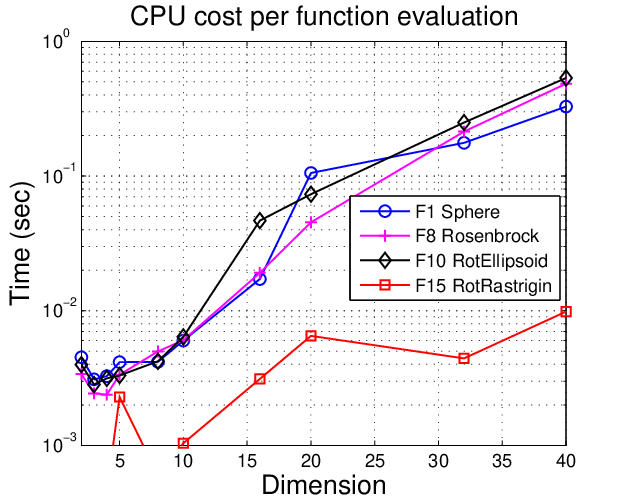
For the timing experiment the IPOP-^s∗aACM-ES was run on noiseless $f_{1}$ , $f_{8}$ , $f_{10}$ and $f_{15}$ functions without self-adaptation of surrogate model hyper-parameters. The crucial hyper-parameter for CPU time measurements, the number of training points was set $N_{training}=\left\lfloor 40+4D^{1.7}\right\rfloor$ as a function of dimension $D$ [14].

These experiments have been conducted on a single core with 2.4 GHz under Windows XP using Matlab R2006a.

On uni-modal functions the time complexity of surrogate model learning increases cubically in the search space dimension (see Fig. 1) and quadratically in the number of training points. For small dimensions ( $D<10$ ) the overall time complexity increases super-linearly in the dimension. The time complexity per function evaluation depends on the population size, because one model is used to estimate the ranking of all points of the population. This leads to a smaller computational complexity on multi-modal functions, e.g. $f_{15}$ Rastrigin function, where the population becomes much larger after several restarts. The time complexity on noisy functions is more similar to the one of Rastrigin function, because in both cases the large populations are used.

The results presented here does not take into account the model hyper-parameters optimization, where $\lambda_{hyp}$ surrogate models should be build at each iteration, which leads to an increase of CPU time per function evaluation by a factor of $\lambda_{hyp}$ . For IPOP-^s∗aACM-ES $\lambda_{hyp}$ was set to 20.

Refer to caption — Figure 1: CPU cost per function evaluation of IPOP-aACM-ES with fixed hyper-parameters.

5 Conclusion

In this paper, we have compared the recently proposed self-adaptive surrogate-assisted IPOP-^s∗aACM-ES with the IPOP-aCMA-ES on noisy benchmark problems. The surrogate-assisted IPOP-^s∗aACM-ES algorithm outperforms the original IPOP-aCMA-ES by a factor from 2 to 3 on the functions with moderate noise, and usually performs not worse on other functions. The IPOP-^s∗aACM-ES algorithm improves the records on 15 out of 30 functions in dimension 20.

6 ACKNOWLEDGMENTS

The authors would like to acknowledge Anne Auger, Zyed Bouzarkouna, Nikolaus Hansen and Thomas P. Runarsson for their valuable discussions. This work was partially funded by FUI of System@tic Paris-Region ICT cluster through contract DGT 117 407 Complex Systems Design Lab (CSDL).

$\Delta f_{\mathrm{opt}}$ 1e1 1e0 1e-1 1e-3 1e-5 1e-7 #succ f101 11 37 44 62 69 75 15 /15 IPOP-aC 3 .0(2) 3 .0(1) 4 .2(1) 5 .8(2) 7 .6(2) 9 .3(2) 15 /15 IPOP-sa 1 .9(1) 2 .1(0.5)^⋆ 2 .2(0.5)^⋆3 2 .2(0.5)^⋆4 2 .5(0.3)^⋆4 2 .8(0.3)^⋆4 15 /15 $\Delta f_{\mathrm{opt}}$ 1e1 1e0 1e-1 1e-3 1e-5 1e-7 #succ f102 11 35 50 72 86 99 15 /15 IPOP-aC 3 .5(3) 3 .4(1) 3 .8(0.9) 5 .0(0.6) 6 .1(0.8) 7 .0(0.7) 15 /15 IPOP-sa 2 .6(2) 2 .1(0.7) 2 .0(0.5)^⋆4 1 .9(0.4)^⋆4 2 .1(0.3)^⋆4 2 .2(0.3)^⋆4 15 /15 $\Delta f_{\mathrm{opt}}$ 1e1 1e0 1e-1 1e-3 1e-5 1e-7 #succ f103 11 28 30 31 35 115 15 /15 IPOP-aC 2 .9(1) 4 .1(1) 6 .3(1) 11 (2) 16 (2) 6 .5(0.6) 15 /15 IPOP-sa 3 .0(1) 2 .8(0.7)^⋆ 3 .4(0.9)^⋆3 4 .6(1)^⋆4 7 .1(3)^⋆4 3 .2(1)^⋆4 15 /15 $\Delta f_{\mathrm{opt}}$ 1e1 1e0 1e-1 1e-3 1e-5 1e-7 #succ f104 173 773 1287 1768 2040 2284 15 /15 IPOP-aC 1 .5(0.5) 2 .0(2) 1 .7(1) 1 .6(1.0) 1 .5(0.9) 1 .4(0.8) 15 /15 IPOP-sa 0 .88(0.3)^⋆ 1 .5(1) 1 .1(1) 0 .89(0.8) 0 .80(0.7)^⋆ 0 .73(0.7)^⋆ 15 /15 $\Delta f_{\mathrm{opt}}$ 1e1 1e0 1e-1 1e-3 1e-5 1e-7 #succ f105 167 1436 5174 10388 10824 11202 15 /15 IPOP-aC 2 .8(0.5) 3 .0(2) 1 .3(0.8) 0 .70(0.4) 0 .70(0.4) 0 .70(0.4) 15 /15 IPOP-sa 1 .4(0.5) 1 .5(2) 0 .63(0.4) 0 .33(0.2) ${}^{\star}_{\downarrow 3}$ 0 .32(0.2) ${}^{\star}_{\downarrow 3}$ 0 .32(0.2) ${}^{\star}_{\downarrow 3}$ 15 /15 $\Delta f_{\mathrm{opt}}$ 1e1 1e0 1e-1 1e-3 1e-5 1e-7 #succ f106 92 529 1050 2666 2887 3087 15 /15 IPOP-aC 2 .3(0.7) 1 .9(0.6) 1 .6(0.3) 0 .87(0.1) 0 .90(0.1) 0 .92(0.1) 15 /15 IPOP-sa 1 .7(0.9) 0 .89(0.2)^⋆2 0 .60(0.2)^⋆2 0 .30(0.1) ${}^{\star 3}_{\downarrow 4}$ 0 .32(0.1) ${}^{\star 3}_{\downarrow 4}$ 0 .36(0.1) ${}^{\star 3}_{\downarrow 4}$ 15 /15 $\Delta f_{\mathrm{opt}}$ 1e1 1e0 1e-1 1e-3 1e-5 1e-7 #succ f107 40 228 453 940 1376 1850 15 /15 IPOP-aC 1 .9(2) 2 .8(4) 1 .9(2) 1 .4(1.0) 1 .3(0.7) 1 .4(0.7) 15 /15 IPOP-sa 1 .4(2) 1 .1(0.7) 1 .4(1) 1 .3(0.8) 1 .4(1.0) 1 .9(1) 15 /15 $\Delta f_{\mathrm{opt}}$ 1e1 1e0 1e-1 1e-3 1e-5 1e-7 #succ f108 87 5144 14469 30935 58628 80667 15 /15 IPOP-aC 11 (17) 0 .68(0.5) 0 .64(0.2) 0 .64(0.4) 0 .66(0.3) 0 .94(0.5) 15 /15 IPOP-sa 7 .8(9) 1 .1(1) 0 .60(0.4) 0 .80(0.5) 0 .74(0.4) 1 .0(0.6) 15 /15 $\Delta f_{\mathrm{opt}}$ 1e1 1e0 1e-1 1e-3 1e-5 1e-7 #succ f109 11 57 216 572 873 946 15 /15 IPOP-aC 3 .1(2) 1 .9(0.6) 1 .1(0.3) 0 .92(0.2) 1 .2(0.2) 1 .5(0.3) 15 /15 IPOP-sa 2 .9(2) 1 .6(0.6) 0 .83(0.3) 1 .2(0.3) 1 .2(0.3) 1 .6(0.4) 15 /15 $\Delta f_{\mathrm{opt}}$ 1e1 1e0 1e-1 1e-3 1e-5 1e-7 #succ f110 949 33625 1.2e5 5.9e5 6.0e5 6.1e5 15 /15 IPOP-aC 0 .54(0.7) 4 .3(5) 3 .2(3) 0 .79(0.8) 0 .79(0.8) 0 .79(0.8) 15 /15 IPOP-sa 0 .71(0.3) 5 .6(7) 3 .5(4) 0 .78(0.8) 0 .84(0.8) 0 .84(0.8) 15 /15 $\Delta f_{\mathrm{opt}}$ 1e1 1e0 1e-1 1e-3 1e-5 1e-7 #succ f111 6856 6.1e5 8.8e6 2.3e7 3.1e7 3.1e7 3 /15 IPOP-aC 0 .54(0.4) 7 .3(8) 7 .9(9) $\infty$ $\infty$ $\infty$ 5e6 0 /15 IPOP-sa 0 .50(0.3) 7 .4(8) 1 .8(2) 1 .00(1) 0 .74(0.7) 0 .74(0.6) 3 /15 $\Delta f_{\mathrm{opt}}$ 1e1 1e0 1e-1 1e-3 1e-5 1e-7 #succ f112 107 1684 3421 4502 5132 5596 15 /15 IPOP-aC 2 .2(0.6) 1 .2(0.6) 1 .0(0.5) 1 .1(0.3) 1 .1(0.3) 1 .1(0.3) 15 /15 IPOP-sa 1 .4(0.6)^⋆2 1 .5(2) 1 .2(0.9) 1 .2(0.6) 1 .2(0.6) 1 .2(0.6) 15 /15 $\Delta f_{\mathrm{opt}}$ 1e1 1e0 1e-1 1e-3 1e-5 1e-7 #succ f113 133 1883 8081 24128 24128 24402 15 /15 IPOP-aC 4 .4(6) 0 .78(1) 0 .77(0.7) 0 .32(0.2) 0 .32(0.2) 0 .32(0.3) 15 /15 IPOP-sa 3 .0(2) 0 .82(0.8) 0 .47(0.6) 0 .35(0.4) 0 .35(0.4) 0 .35(0.4) 15 /15 $\Delta f_{\mathrm{opt}}$ 1e1 1e0 1e-1 1e-3 1e-5 1e-7 #succ f114 767 14720 56311 83272 83272 84949 15 /15 IPOP-aC 3 .3(3) 0 .61(0.5) 0 .49(0.3) 0 .60(0.2) 0 .60(0.2) 0 .61(0.2) 15 /15 IPOP-sa 2 .6(3) 0 .73(0.4) 0 .54(0.4) 0 .44(0.2) 0 .44(0.2) 0 .44(0.3) 15 /15 $\Delta f_{\mathrm{opt}}$ 1e1 1e0 1e-1 1e-3 1e-5 1e-7 #succ f115 64 485 1829 2550 2550 2970 15 /15 IPOP-aC 1 .8(1.0) 0 .81(0.9) 1 .1(1) 1 .4(1) 1 .4(1) 1 .5(1) 15 /15 IPOP-sa 1 .6(0.6) 0 .98(1) 1 .2(1) 1 .2(0.8) 1 .2(0.8) 1 .1(0.7) 15 /15 $\Delta f_{\mathrm{opt}}$ 1e1 1e0 1e-1 1e-3 1e-5 1e-7 #succ f116 5730 14472 22311 26868 30329 31661 15 /15 IPOP-aC 0 .88(0.8) 0 .62(0.6) 0 .57(0.4) 0 .73(0.5) 0 .68(0.4) 0 .68(0.4) 15 /15 IPOP-sa 1 .0(1) 0 .74(0.8) 0 .56(0.5) 0 .59(0.5) 0 .56(0.4)_↓ 0 .56(0.4)_↓ 15 /15 $\Delta f_{\mathrm{opt}}$ 1e1 1e0 1e-1 1e-3 1e-5 1e-7 #succ f117 26686 76052 1.1e5 1.4e5 1.7e5 1.9e5 15 /15 IPOP-aC 0 .65(0.5) 0 .48(0.4) 0 .44(0.2)_↓2 0 .47(0.2)_↓2 0 .43(0.2)_↓2 0 .46(0.2)_↓2 15 /15 IPOP-sa 0 .60(0.5) 0 .43(0.3) 0 .42(0.3)_↓2 0 .54(0.3)_↓ 0 .59(0.3) 0 .60(0.2) 15 /15 $\Delta f_{\mathrm{opt}}$ 1e1 1e0 1e-1 1e-3 1e-5 1e-7 #succ f118 429 1217 1555 1998 2430 2913 15 /15 IPOP-aC 1 .7(0.6) 0 .88(0.3) 0 .91(0.2) 0 .91(0.1) 0 .91(0.1) 0 .90(0.1) 15 /15 IPOP-sa 0 .49(0.1) ${}^{\star 4}_{\downarrow 4}$ 0 .25(0.1) ${}^{\star 4}_{\downarrow 4}$ 0 .33(0.1) ${}^{\star 4}_{\downarrow 4}$ 0 .48(0.1) ${}^{\star 4}_{\downarrow 4}$ 0 .63(0.1) ${}^{\star 2}_{\downarrow 3}$ 0 .74(0.3) ${}^{\star}_{\downarrow 2}$ 15 /15 $\Delta f_{\mathrm{opt}}$ 1e1 1e0 1e-1 1e-3 1e-5 1e-7 #succ f119 12 657 1136 10372 35296 49747 15 /15 IPOP-aC 1 .5(1) 0 .55(0.6) 0 .58(0.5) 0 .55(0.4) 0 .49(0.2)_↓2 0 .61(0.4) 15 /15 IPOP-sa 4 .9(10) 1 .1(2) 0 .99(0.9) 0 .50(0.5) 0 .47(0.2)_↓2 0 .61(0.5) 15 /15 $\Delta f_{\mathrm{opt}}$ 1e1 1e0 1e-1 1e-3 1e-5 1e-7 #succ f120 16 2900 18698 72438 3.3e5 5.5e5 15 /15 IPOP-aC 18 (39) 0 .76(1) 0 .65(0.5) 0 .83(0.5) 0 .43(0.3)_↓2 0 .66(0.5) 15 /15 IPOP-sa 26 (56) 1 .1(1) 0 .80(0.5) 0 .52(0.3) 0 .36(0.3)_↓3 0 .64(0.5) 15 /15 $\Delta f_{\mathrm{opt}}$ 1e1 1e0 1e-1 1e-3 1e-5 1e-7 #succ f121 8.6 111 273 1583 3870 6195 15 /15 IPOP-aC 3 .0(3) 1 .1(0.4) 1 .1(0.3) 0 .78(0.3) 0 .84(0.1) 0 .82(0.1)_↓ 15 /15 IPOP-sa 3 .3(4) 0 .98(0.5) 0 .97(0.5) 1 .0(0.6) 0 .95(0.4) 0 .86(0.2) 15 /15 $\Delta f_{\mathrm{opt}}$ 1e1 1e0 1e-1 1e-3 1e-5 1e-7 #succ f122 10 1727 9190 30087 53743 1.1e5 15 /15 IPOP-aC 2 .9(3) 1 .4(1) 0 .71(0.6) 0 .48(0.2)_↓2 0 .66(0.3) 0 .58(0.5)_↓2 15 /15 IPOP-sa 2 .6(3) 1 .2(0.8) 0 .75(0.5) 0 .58(0.2)_↓ 0 .77(0.3) 0 .66(0.3)_↓ 15 /15 $\Delta f_{\mathrm{opt}}$ 1e1 1e0 1e-1 1e-3 1e-5 1e-7 #succ f123 11 16066 81505 3.4e5 6.7e5 2.2e6 15 /15 IPOP-aC 28 (60) 0 .94(0.7) 0 .66(0.4) 0 .67(0.4) 0 .56(0.2)_↓2 0 .60(0.3) 15 /15 IPOP-sa 23 (52) 0 .74(0.4) 0 .70(0.5) 0 .58(0.3) 0 .80(0.7) 0 .71(0.5) 15 /15 $\Delta f_{\mathrm{opt}}$ 1e1 1e0 1e-1 1e-3 1e-5 1e-7 #succ f124 10 202 1040 20478 45337 95200 15 /15 IPOP-aC 2 .6(3) 1 .2(0.8) 2 .1(3) 0 .93(0.6) 0 .94(0.5) 0 .59(0.3) 15 /15 IPOP-sa 2 .6(2) 1 .3(0.6) 3 .1(4) 0 .85(0.7) 0 .97(0.8) 4 .1(8) 15 /15 $\Delta f_{\mathrm{opt}}$ 1e1 1e0 1e-1 1e-3 1e-5 1e-7 #succ f125 1 1 1 2.4e5 2.4e5 2.5e5 15 /15 IPOP-aC 1 (0) 26 (22) 3142 (3751) 0 .53(0.4) 0 .57(0.4) 0 .57(0.4) 15 /15 IPOP-sa 1 .5(0) 18 (18) 4308 (4084) 0 .56(0.6) 0 .79(0.9) 4 .8(6) 15 /15 $\Delta f_{\mathrm{opt}}$ 1e1 1e0 1e-1 1e-3 1e-5 1e-7 #succ f126 1 1 1 $\infty$ $\infty$ $\infty$ 0 IPOP-aC 1 (0) 62 (98) 7882 (5858) . . . 0 /15 IPOP-sa 1 (0) 165 (444) 9361 (8720) 1.3e7(1e7) 1.3e7(2e7) 1.3e7(1e7) 5 /15 $\Delta f_{\mathrm{opt}}$ 1e1 1e0 1e-1 1e-3 1e-5 1e-7 #succ f127 1 1 1 3.4e5 3.9e5 4.0e5 15 /15 IPOP-aC 1 .1(0) 30 (24) 3085 (2864) 0 .50(0.5) 0 .46(0.4) 0 .46(0.4) 15 /15 IPOP-sa 1 (0) 20 (22) 2432 (3044) 0 .30(0.3) 0 .32(0.3)_↓ 0 .33(0.3)_↓ 15 /15 $\Delta f_{\mathrm{opt}}$ 1e1 1e0 1e-1 1e-3 1e-5 1e-7 #succ f128 111 4248 7808 12447 17217 21162 15 /15 IPOP-aC 2 .6(1) 1 .8(2) 47 (2) 30 (3) 22 (2) 18 (2) 14 /15 IPOP-sa 1 .3(1.0) 16 (21) 265 (331) 203 (342) 147 (152) 124 (212) 11 /15 $\Delta f_{\mathrm{opt}}$ 1e1 1e0 1e-1 1e-3 1e-5 1e-7 #succ f129 64 10710 59443 2.8e5 5.1e5 5.8e5 15 /15 IPOP-aC 11 (16) 10 (5) 16 (27) 7 .0(8) 3 .9(7) 3 .5(6) 10 /15 IPOP-sa 9 .1(12) 10 (21) 19 (42) 13 (18) 7 .1(10) 6 .3(9) 9 /15 $\Delta f_{\mathrm{opt}}$ 1e1 1e0 1e-1 1e-3 1e-5 1e-7 #succ f130 55 812 3034 32823 33889 34528 10 /15 IPOP-aC 1 .4(0.8) 143 (288) 391 (625) 36 (46) 35 (45) 35 (44) 11 /15 IPOP-sa 1 .4(0.9) 27 (27) 126 (131) 42 (76) 41 (74) 40 (72) 13 /15

Table 1: Expected running time (ERT in number of function evaluations) divided by the respective best ERT measured during BBOB-2009 (given in the respective first row) for different

\Delta f

values in dimension

5

. The central 80% range divided by two is given in braces. The median number of conducted function evaluations is additionally given in italics, if

\mathrm{ERT}(10^{-7})=\infty

. #succ is the number of trials that reached the final target

f_{\mathrm{opt}}+10^{-8}

. Best results are printed in bold.

$\Delta f_{\mathrm{opt}}$ 1e1 1e0 1e-1 1e-3 1e-5 1e-7 #succ f101 59 425 571 700 739 783 15 /15 IPOP-aC 6 .1(1.0) 1 .5(0.1) 1 .6(0.1) 2 .1(0.2) 2 .7(0.1) 3 .3(0.2) 15 /15 IPOP-sa 4 .7(1)^⋆ 0 .86(0.2)^⋆4 0 .73(0.1) ${}^{\star 4}_{\downarrow 2}$ 0 .78(0.1) ${}^{\star 4}_{\downarrow 3}$ 0 .88(0.1) ${}^{\star 4}_{\downarrow}$ 0 .99(0.1)^⋆4 15 /15 $\Delta f_{\mathrm{opt}}$ 1e1 1e0 1e-1 1e-3 1e-5 1e-7 #succ f102 231 399 579 921 1157 1407 15 /15 IPOP-aC 1 .5(0.4) 1 .6(0.2) 1 .6(0.2) 1 .6(0.1) 1 .7(0.1) 1 .8(0.1) 15 /15 IPOP-sa 1 .2(0.2) 0 .93(0.2)^⋆4 0 .75(0.1) ${}^{\star 4}_{\downarrow 3}$ 0 .61(0.1) ${}^{\star 4}_{\downarrow 4}$ 0 .60(0.0) ${}^{\star 4}_{\downarrow 4}$ 0 .60(0.0) ${}^{\star 4}_{\downarrow 4}$ 15 /15 $\Delta f_{\mathrm{opt}}$ 1e1 1e0 1e-1 1e-3 1e-5 1e-7 #succ f103 65 417 629 1313 1893 2464 14 /15 IPOP-aC 5 .4(0.9) 1 .5(0.1) 1 .5(0.1) 1 .2(0.1) 1 .2(0.1) 1 .2(0.1) 15 /15 IPOP-sa 3 .9(0.8)^⋆2 0 .83(0.2) ${}^{\star 4}_{\downarrow 2}$ 0 .66(0.1)^⋆4 0 .52(0.1) ${}^{\star 4}_{\downarrow 4}$ 0 .55(0.1) ${}^{\star 4}_{\downarrow 4}$ 0 .58(0.1) ${}^{\star 4}_{\downarrow 3}$ 15 /15 $\Delta f_{\mathrm{opt}}$ 1e1 1e0 1e-1 1e-3 1e-5 1e-7 #succ f104 23690 85656 1.7e5 1.8e5 1.9e5 2.0e5 15 /15 IPOP-aC 4 .9(3) 1 .6(1.0) 0 .82(0.5) 0 .80(0.5) 0 .79(0.5) 0 .77(0.4) 15 /15 IPOP-sa 3 .5(2) 1 .1(0.6) 0 .55(0.3) 0 .52(0.3) 0 .50(0.3) 0 .49(0.3) 15 /15 $\Delta f_{\mathrm{opt}}$ 1e1 1e0 1e-1 1e-3 1e-5 1e-7 #succ f105 1.9e5 6.1e5 6.3e5 6.5e5 6.6e5 6.7e5 15 /15 IPOP-aC 1 .2(0.3) 0 .43(0.1)_↓3 0 .43(0.1)_↓3 0 .44(0.1)_↓3 0 .44(0.1)_↓3 0 .44(0.1)_↓3 15 /15 IPOP-sa 1 .0(0.4) 0 .36(0.1)_↓3 0 .35(0.1)_↓3 0 .34(0.1)_↓3 0 .34(0.1)_↓3 0 .33(0.1)_↓3 15 /15 $\Delta f_{\mathrm{opt}}$ 1e1 1e0 1e-1 1e-3 1e-5 1e-7 #succ f106 11480 21668 23746 25470 26492 27360 15 /15 IPOP-aC 0 .77(0.2) 0 .76(0.2)_↓3 0 .84(0.2)_↓2 0 .89(0.1) 0 .91(0.1) 0 .91(0.1) 15 /15 IPOP-sa 0 .28(0.1) ${}^{\star 4}_{\downarrow 4}$ 0 .37(0.3) ${}^{\star 2}_{\downarrow 4}$ 0 .39(0.2) ${}^{\star 3}_{\downarrow 4}$ 0 .45(0.2) ${}^{\star 3}_{\downarrow 4}$ 0 .46(0.2) ${}^{\star 3}_{\downarrow 4}$ 0 .47(0.2) ${}^{\star 3}_{\downarrow 4}$ 15 /15 $\Delta f_{\mathrm{opt}}$ 1e1 1e0 1e-1 1e-3 1e-5 1e-7 #succ f107 8571 13582 16226 27357 52486 65052 15 /15 IPOP-aC 0 .81(0.4) 0 .97(0.4) 1 .3(0.6) 1 .5(0.9) 1 .3(0.7) 1 .1(0.5) 15 /15 IPOP-sa 0 .83(0.5) 1 .3(0.8) 1 .4(0.7) 1 .3(0.8) 1 .0(0.5) 0 .94(0.4) 15 /15 $\Delta f_{\mathrm{opt}}$ 1e1 1e0 1e-1 1e-3 1e-5 1e-7 #succ f108 58063 97228 2.0e5 4.5e5 6.3e5 9.0e5 15 /15 IPOP-aC 0 .74(0.3) 0 .98(0.5) 1 .0(0.6) 1 .1(0.6) 1 .5(0.4) 1 .5(0.3) 15 /15 IPOP-sa 0 .72(0.3) 1 .2(0.6) 1 .1(0.6) 1 .2(0.7) 1 .6(0.3) 1 .4(0.3) 15 /15 $\Delta f_{\mathrm{opt}}$ 1e1 1e0 1e-1 1e-3 1e-5 1e-7 #succ f109 333 632 1138 2287 3583 4952 15 /15 IPOP-aC 1 .1(0.2) 1 .2(0.1) 1 .2(0.2) 1 .2(0.1) 1 .1(0.1) 1 .1(0.1) 15 /15 IPOP-sa 0 .93(0.3) 0 .78(0.2) ${}^{\star 3}_{\downarrow}$ 0 .78(0.2) ${}^{\star 3}_{\downarrow 2}$ 0 .89(0.3)^⋆ 0 .79(0.2) ${}^{\star 3}_{\downarrow}$ 0 .75(0.2) ${}^{\star 3}_{\downarrow 2}$ 15 /15 $\Delta f_{\mathrm{opt}}$ 1e1 1e0 1e-1 1e-3 1e-5 1e-7 #succ f110 $\infty$ $\infty$ $\infty$ $\infty$ $\infty$ $\infty$ 0 IPOP-aC . . . . . . 0 /15 IPOP-sa . . . . . . 0 /15 $\Delta f_{\mathrm{opt}}$ 1e1 1e0 1e-1 1e-3 1e-5 1e-7 #succ f111 $\infty$ $\infty$ $\infty$ $\infty$ $\infty$ $\infty$ 0 IPOP-aC . . . . . . 0 /15 IPOP-sa . . . . . . 0 /15 $\Delta f_{\mathrm{opt}}$ 1e1 1e0 1e-1 1e-3 1e-5 1e-7 #succ f112 25552 64124 69621 73557 76137 78238 15 /15 IPOP-aC 0 .84(0.2) 0 .84(0.5) 0 .89(0.5) 0 .93(0.5) 0 .94(0.5) 0 .93(0.4) 15 /15 IPOP-sa 0 .89(0.3) 0 .79(0.1) 0 .84(0.1) 0 .88(0.1) 0 .88(0.1) 0 .88(0.1) 15 /15 $\Delta f_{\mathrm{opt}}$ 1e1 1e0 1e-1 1e-3 1e-5 1e-7 #succ f113 50123 3.6e5 5.6e5 5.9e5 5.9e5 5.9e5 15 /15 IPOP-aC 0 .60(0.4) 0 .27(0.1)_↓3 0 .27(0.1)_↓4 0 .29(0.1)_↓4 0 .29(0.1)_↓4 0 .29(0.1)_↓4 15 /15 IPOP-sa 0 .54(0.2) 0 .35(0.2)_↓2 0 .31(0.1)_↓4 0 .32(0.1)_↓4 0 .32(0.1)_↓4 0 .32(0.1)_↓4 15 /15 $\Delta f_{\mathrm{opt}}$ 1e1 1e0 1e-1 1e-3 1e-5 1e-7 #succ f114 2.1e5 1.1e6 1.4e6 1.6e6 1.6e6 1.6e6 15 /15 IPOP-aC 0 .64(0.5) 0 .35(0.1)_↓4 0 .53(0.3)_↓ 0 .62(0.3) 0 .62(0.3) 0 .63(0.3) 15 /15 IPOP-sa 0 .71(0.3) 0 .39(0.3)_↓3 0 .40(0.2)_↓3 0 .50(0.3)_↓2 0 .50(0.3)_↓2 0 .55(0.3)_↓ 15 /15 $\Delta f_{\mathrm{opt}}$ 1e1 1e0 1e-1 1e-3 1e-5 1e-7 #succ f115 2405 30268 91749 1.3e5 1.3e5 1.3e5 15 /15 IPOP-aC 1 .4(2) 1 .2(0.6) 0 .54(0.1) 0 .45(0.0)_↓4 0 .45(0.0)_↓4 0 .45(0.1)_↓4 15 /15 IPOP-sa 0 .75(2) 0 .67(0.3) 0 .31(0.2)^⋆2 4 .8(15) 4 .8(15) 4 .7(14) 15 /15 $\Delta f_{\mathrm{opt}}$ 1e1 1e0 1e-1 1e-3 1e-5 1e-7 #succ f116 5.0e5 6.9e5 8.9e5 1.0e6 1.1e6 1.1e6 15 /15 IPOP-aC 0 .36(0.1) 0 .28(0.1)_↓ 0 .23(0.0)_↓2 0 .22(0.0)_↓4 0 .23(0.0)_↓4 0 .24(0.0)_↓4 15 /15 IPOP-sa 0 .46(0.1) 0 .35(0.1) 0 .30(0.1) 0 .28(0.1)_↓4 0 .29(0.1)_↓4 0 .30(0.1)_↓4 15 /15 $\Delta f_{\mathrm{opt}}$ 1e1 1e0 1e-1 1e-3 1e-5 1e-7 #succ f117 1.8e6 2.5e6 2.6e6 2.9e6 3.2e6 3.6e6 15 /15 IPOP-aC 0 .37(0.2)_↓2 0 .35(0.2)_↓4 0 .41(0.3)_↓3 0 .45(0.2)_↓3 0 .47(0.2)_↓3 0 .56(0.3)_↓3 15 /15 IPOP-sa 0 .29(0.1)_↓3 0 .26(0.1)_↓4 0 .29(0.1)_↓4 0 .35(0.2)_↓4 0 .42(0.2)_↓3 0 .48(0.4)_↓2 15 /15 $\Delta f_{\mathrm{opt}}$ 1e1 1e0 1e-1 1e-3 1e-5 1e-7 #succ f118 6908 11786 17514 26342 30062 32659 15 /15 IPOP-aC 0 .82(0.1) 0 .78(0.2) 0 .71(0.2) 0 .63(0.1)_↓3 0 .64(0.1)_↓4 0 .66(0.1)_↓3 15 /15 IPOP-sa 0 .42(0.2) ${}^{\star 3}_{\downarrow 4}$ 0 .49(0.1) ${}^{\star 3}_{\downarrow 4}$ 0 .54(0.1) ${}^{\star}_{\downarrow 3}$ 0 .54(0.2)_↓4 0 .56(0.1)_↓4 0 .58(0.1) ${}^{\star}_{\downarrow 4}$ 15 /15 $\Delta f_{\mathrm{opt}}$ 1e1 1e0 1e-1 1e-3 1e-5 1e-7 #succ f119 2771 29365 35930 4.1e5 1.4e6 1.9e6 15 /15 IPOP-aC 1 .6(1) 0 .62(0.4) 0 .83(0.4) 0 .42(0.3)_↓2 0 .25(0.1)_↓4 0 .28(0.1)_↓4 15 /15 IPOP-sa 1 .5(2) 0 .74(0.3) 0 .88(0.3) 0 .33(0.1)_↓3 0 .25(0.1)_↓4 0 .37(0.3)_↓3 15 /15 $\Delta f_{\mathrm{opt}}$ 1e1 1e0 1e-1 1e-3 1e-5 1e-7 #succ f120 36040 1.8e5 2.8e5 1.6e6 6.7e6 1.4e7 13 /15 IPOP-aC 0 .62(0.3) 0 .64(0.2) 0 .79(0.4) 0 .78(0.4) 0 .44(0.2)_↓3 0 .40(0.2)_↓3 15 /15 IPOP-sa 0 .65(0.5) 0 .80(0.4) 1 .2(0.6) 0 .87(0.5) 0 .42(0.1)_↓3 0 .39(0.2)_↓3 15 /15 $\Delta f_{\mathrm{opt}}$ 1e1 1e0 1e-1 1e-3 1e-5 1e-7 #succ f121 249 769 1426 9304 34434 57404 15 /15 IPOP-aC 1 .2(0.3) 1 .0(0.2) 1 .1(0.2) 0 .77(0.1)_↓3 0 .56(0.1)_↓4 0 .64(0.1)_↓4 15 /15 IPOP-sa 1 .2(0.4) 0 .85(0.2) 0 .92(0.3) 0 .69(0.1)_↓3 0 .58(0.1)_↓4 0 .71(0.1)_↓3 15 /15 $\Delta f_{\mathrm{opt}}$ 1e1 1e0 1e-1 1e-3 1e-5 1e-7 #succ f122 692 52008 1.4e5 7.9e5 2.0e6 5.8e6 15 /15 IPOP-aC 2 .3(3) 0 .81(0.3) 0 .97(0.6) 0 .56(0.3) 0 .66(0.1) 0 .81(0.9) 15 /15 IPOP-sa 2 .5(3) 0 .94(0.6) 0 .81(0.3) 0 .53(0.1)_↓ 0 .51(0.2)_↓ 0 .57(0.3) 15 /15 $\Delta f_{\mathrm{opt}}$ 1e1 1e0 1e-1 1e-3 1e-5 1e-7 #succ f123 1063 5.3e5 1.5e6 5.3e6 2.7e7 1.6e8 0 IPOP-aC 6 .4(4) 0 .72(0.4) 0 .88(0.8) 0 .94(0.7) 0 .50(0.1) 1 .9(2) 0 /15 IPOP-sa 7 .6(8) 0 .77(0.5) 0 .81(0.5) 1 .1(0.7) 0 .63(0.4) 0 .92(1) 0 /15 $\Delta f_{\mathrm{opt}}$ 1e1 1e0 1e-1 1e-3 1e-5 1e-7 #succ f124 192 1959 40840 1.3e5 3.9e5 8.0e5 15 /15 IPOP-aC 1 .1(0.5) 3 .9(11) 1 .0(0.7) 0 .91(0.6) 0 .76(0.4) 0 .62(0.3) 15 /15 IPOP-sa 0 .86(0.4) 3 .0(0.8) 2 .2(2) 1 .4(0.5) 0 .76(0.3) 4 .0(5) 14 /15 $\Delta f_{\mathrm{opt}}$ 1e1 1e0 1e-1 1e-3 1e-5 1e-7 #succ f125 1 1 1 2.5e7 8.0e7 8.1e7 4 /15 IPOP-aC 1 (0) 827 (912) 3.8e6(4e6) 1 .1(1) 1 .7(2) 1 .7(2) 2 /15 IPOP-sa 1 (0) 1083 (1766) 3.3e6(2e6) 0 .61(0.5) 1 .1(1) 1 .1(1) 3 /15 $\Delta f_{\mathrm{opt}}$ 1e1 1e0 1e-1 1e-3 1e-5 1e-7 #succ f126 1 1 1 $\infty$ $\infty$ $\infty$ 0 IPOP-aC 1 (0) 6417 (3982) $\infty$ . . . 0 /15 IPOP-sa 1 (0) 7156 (4580) $\infty$ . . . 0 /15 $\Delta f_{\mathrm{opt}}$ 1e1 1e0 1e-1 1e-3 1e-5 1e-7 #succ f127 1 1 1 4.4e6 7.3e6 7.4e6 15 /15 IPOP-aC 1 (0) 193 (102) 2.8e5(4e5) 1 .0(0.9) 1 .1(1) 1 .1(1.0) 15 /15 IPOP-sa 1 (0) 238 (106) 3.3e5(4e5) 0 .75(0.6) 0 .93(0.5) 0 .97(0.6) 14 /15 $\Delta f_{\mathrm{opt}}$ 1e1 1e0 1e-1 1e-3 1e-5 1e-7 #succ f128 1.4e5 1.3e7 1.7e7 1.7e7 1.7e7 1.7e7 9 /15 IPOP-aC 0 .51(0.6) 0 .72(1) 1 .0(2) 1 .0(2) 1 .0(1) 1 .0(1) 7 /15 IPOP-sa 1 .3(2) 0 .59(0.8) 1 .1(1) 1 .1(2) 1 .1(1) 1 .1(2) 8 /15 $\Delta f_{\mathrm{opt}}$ 1e1 1e0 1e-1 1e-3 1e-5 1e-7 #succ f129 7.8e6 4.1e7 4.2e7 4.2e7 4.2e7 4.2e7 5 /15 IPOP-aC 0 .16(0.2)_↓ 0 .27(0.3) 0 .46(0.6) 0 .46(0.6) 0 .46(0.6) 0 .46(0.6) 6 /15 IPOP-sa 0 .41(0.9) 0 .28(0.5) 0 .36(0.5) 0 .36(0.5) 0 .36(0.5) 0 .36(0.5) 9 /15 $\Delta f_{\mathrm{opt}}$ 1e1 1e0 1e-1 1e-3 1e-5 1e-7 #succ f130 4904 93149 2.5e5 2.5e5 2.6e5 2.6e5 7 /15 IPOP-aC 1 .5(2) 66 (99) 54 (71) 54 (71) 54 (72) 53 (70) 6 /15 IPOP-sa 0 .55(1) 27 (34) 30 (43) 30 (49) 30 (39) 30 (41) 12 /15

Table 2: Expected running time (ERT in number of function evaluations) divided by the respective best ERT measured during BBOB-2009 (given in the respective first row) for different

\Delta f

values in dimension

20

. The central 80% range divided by two is given in braces. The median number of conducted function evaluations is additionally given in italics, if

\mathrm{ERT}(10^{-7})=\infty

. #succ is the number of trials that reached the final target

f_{\mathrm{opt}}+10^{-8}

. Best results are printed in bold.

References

[1] Z. Bouzarkouna, A. Auger, and D. Ding. Investigating the local-meta-model CMA-ES for large population sizes. In C. Di Chio et al., editor, Proc. EvoNUM’10, pages 402–411. LNCS 6024, Springer, 2010.
[2] S. Finck, N. Hansen, R. Ros, and A. Auger. Real-parameter black-box optimization benchmarking 2010: Presentation of the noisy functions. Technical Report 2009/21, Research Center PPE, 2010.
[3] L. Graning, Y. Jin, and B. Sendhoff. Efficient evolutionary optimization using individual-based evolution control and neural networks: A comparative study. In Proc. ESANN’2005, pages 27–29, 2005.
[4] N. Hansen, A. Auger, S. Finck, and R. Ros. Real-parameter black-box optimization benchmarking 2012: Experimental setup. Technical report, INRIA, 2012.
[5] N. Hansen, S. Finck, R. Ros, and A. Auger. Real-parameter black-box optimization benchmarking 2009: Noisy functions definitions. Technical Report RR-6869, INRIA, 2009. Updated February 2010.
[6] N. Hansen and A. Ostermeier. Completely derandomized self-adaptation in evolution strategies. Evolutionary Computation, 9(2):159–195, 2001.
[7] N. Hansen and R. Ros. Benchmarking a weighted negative covariance matrix update on the BBOB-2010 noiseless testbed. In GECCO ’10: Proceedings of the 12th annual conference comp on Genetic and evolutionary computation, pages 1673–1680, New York, NY, USA, 2010. ACM.
[8] F. Hoffmann and S. Holemann. Controlled model assisted evolution strategy with adaptive preselection. In International Symposium on Evolving Fuzzy Systems, pages 182–187. IEEE, 2006.
[9] H. Ingimundardottir and T. Runarsson. Sampling strategies in ordinal regression for surrogate assisted evolutionary optimization. In Proc. ISDA’2011, page To appear, 2011.
[10] G. A. Jastrebski and D. V. Arnold. Improving evolution strategies through active covariance matrix adaptation. In Proc. CEC’2006, pages 2814–2821, 2006.
[11] S. Kern, N. Hansen, and P. Koumoutsakos. Local meta-models for optimization using evolution strategies. In Th. Runarsson et al., editor, PPSN IX, pages 939–948. LNCS 4193, Springer, 2006.
[12] O. Kramer. Covariance matrix self-adaptation and kernel regression - perspectives of evolutionary optimization in kernel machines. Fundam. Inf., 98:87–106, 2010.
[13] I. Loshchilov, M. Schoenauer, and M. Sebag. Comparison-Based Optimizers Need Comparison-Based Surrogates. In J. K. R. Schaefer, C. Cotta and G. Rudolph, editors, Proc. PPSN XI, pages 364–373. LNCS 6238, Springer, 2010.
[14] I. Loshchilov, M. Schoenauer, and M. Sebag. Self-Adaptive Surrogate-Assisted Covariance Matrix Adaptation Evolution Strategy. In GECCO ’12: Proceedings of the 14th annual conference on Genetic and evolutionary computation, page to appear, New York, NY, USA, 2012. ACM.
[15] K. Price. Differential evolution vs. the functions of the second ICEO. In Proceedings of the IEEE International Congress on Evolutionary Computation, pages 153–157, 1997.
[16] T. P. Runarsson. Ordinal regression in evolutionary computation. In Th. Runarsson et al., editor, PPSN IX, pages 1048–1057. LNCS 4193, Springer, 2006.
[17] H. Ulmer, F. Streichert, and A. Zell. Evolution strategies assisted by gaussian processes with improved pre-selection criterion. In Proc. CEC’2003, pages 692–699, 2003.

all functions	moderate noise
3 IPOP-^s∗aACM best 2009 IPOP-aCMA	3 IPOP-^s∗aACM IPOP-aCMA best 2009
severe noise	severe noise multimod.
3 IPOP-^s∗aACM best 2009 IPOP-aCMA	3 IPOP-^s∗aACM best 2009 IPOP-aCMA

all functions	moderate noise
3 best 2009 IPOP-^s∗aACM IPOP-aCMA	3 IPOP-^s∗aACM IPOP-aCMA best 2009
severe noise	severe noise multimod.
3 IPOP-^s∗aACM IPOP-aCMA best 2009	3 best 2009 IPOP-^s∗aACM IPOP-aCMA

Black-box optimization benchmarking of IPOP-saACM-ES on the BBOB-2012 noisy testbed

Abstract

Keywords:

category

keywords

category

keywords

1 Introduction

2 The Algorithms

2.1 The $(\mu/\mu_{w},\lambda)$ -CMA-ES

2.2 The ^s∗ACM-ES

2.3 The Benchmarked Algorithms

3 Results

4 CPU TIMING EXPERIMENT

5 Conclusion

6 ACKNOWLEDGMENTS

References

Black-box optimization benchmarking of IPOP-saACM-ES on the BBOB-2012 noisy testbed

Abstract

Keywords:

category

keywords

category

keywords

1 Introduction

2 The Algorithms

2.1 The (μ/μw,λ)(\mu/\mu_{w},\lambda)-CMA-ES

2.2 The s∗ACM-ES

2.3 The Benchmarked Algorithms

3 Results

4 CPU TIMING EXPERIMENT

5 Conclusion

6 ACKNOWLEDGMENTS

References

2.1 The $(\mu/\mu_{w},\lambda)$ -CMA-ES

2.2 The ^s∗ACM-ES