Phase structure for lattice fermions
with flavored chemical potential terms

The famous no-go theorem [1, 2] states that lattice fermion actions with chiral symmetry, locality and other common features must produce massless degrees of freedom in multiples of two in a continuum limit. This is contradictory with a phenomenological fact that there exist only three quarks with masses below the QCD scale. By now several fermion constructions to bypass the no-go theorem have been developed, although all of them have their individual shortcomings: The explicit chiral symmetry breaking with the Wilson fermion approach [3] results in an additive mass renormalization, which in turn requires a fine-tuning of the mass parameter for QCD simulations. Domain-wall [4, 5] and overlap fermions [6, 7] produce a single fermion mode by modifying the definition of chiral symmetry or introducing the momentum-dependent chiral charge, although they lead to rather expensive simulations algorithms.. These approaches attempt to realize single fermionic degrees of freedom by breaking the requisite conditions for the no-go theorem. On the other hand, there is another direction to approach numerical simulations. According to [1], Hypercubic symmetry and reflection positivity of actions result in $2^{d}$ species of fermions where $d$ stands for the dimension. Thus it is potentially possible to reduce the number of species by breaking hypercubic symmetry properly. Actually, the staggered fermion approach [8, 9, 10, 11, 12], with only 4 species of fermions does this and possesses flavored-hypercubic symmetry instead. However this requires rooting procedures for the physical $2$ or $(2+1)$-flavor QCD simulation.

A possible goal in this direction is a lattice fermion with $2$ species, the minimal number required by the no-go theorem. Such a minimal-doubling action was first proposed by Karsten, and later by Wilczek [13, 14]. Other than the original type, two more types are known as Creutz-Borici type [15, 16, 17] and Twisted-ordering type [18]. These fermions all possess one exact chiral symmetry and ultra locality. As such they could be faster for simulation, at least for two-flavor QCD, than other chirally symmetric lattice fermions. However it has been shown [19, 20, 21, 22] that we need to fine-tune several parameters for a continuum limit with these actions. This is because they lack sufficient discrete symmetry to prohibit redundant operators from being generated through loop corrections [23, 24, 25, 26]. Thus the minimally doubled fermions have not been extensively used so far. Nevertheless, there is the possibility to apply them to simulations if one can efficiently perform the necessary fine-tuning of parameters.

In this paper we pursue the chiral phase structure in the parameter plane for minimal-doubling lattice QCD for two purposes: One purpose is to understand properties of these formulations theoretically. The other purpose is to show their applicability to lattice QCD simulations since understanding a nontrivial phase diagram, as with the Aoki phase in Wilson fermion [27, 28, 29, 30, 31], can be useful in showing the applicability to lattice QCD. We first show that minimal-doubling fermions can be seen as a special case of lattice fermions with species-dependent (imaginary) chemical potential terms. We focus on the Karsten-Wilczek formulation with one relevant parameter $\mu_{3}$, which corresponds to a mass parameter in the analogy of Wilson fermion. We next investigate the chiral phase structure in the space of the gauge coupling and this relevant parameter. We analyze strong-coupling lattice QCD, and show that chiral symmetry is spontaneously broken in a certain range of the parameter while the chiral condensate is zero outside the range. We find a second-order phase transition between these chiral symmetric and broken phases. We also show that pion becomes massless as a Nambu-Goldstone boson in the chiral-broken phase while the sigma meson becomes massless on the second-order phase boundary due to the critical behavior of the second-order phase transition. We investigate the lattice Gross-Neveu model to capture an entire phase structure. From these results we suppose a similar chiral phase structure in 4d QCD with flavored-chemical-potential lattice fermions, and discuss their applicability to lattice QCD simulations.

In Sec. II, we study lattice fermions with flavored chemical potential, or minimal-doubling fermions. In Sec. III, we investigate a chiral phase structure in the framework of strong-coupling lattice QCD. In Sec. IV, we study the Gross-Neveu model to obtain information of the whole phase diagram. In Sec. V, we discuss a phase structure in 4d QCD from the results of the last two sections. Section VI is devoted to a summary and discussion.

In this section we study minimal-doubling fermions and their generalization. Before going to the main theme, let us remind ourselves of Wilson’s prescription to shirk the no-go theorem. Wilson fermion extracts one light fermion by introducing a species-dependent mass term, which we call a “flavored-mass term”. A free action and a Dirac operator of Wilson fermion are given by

$$S_{\rm W}\,=\,a^{4}\sum_{n,\mu}\bar{\psi}_{n}\gamma_{\mu}{\psi_{n+\mu}-\psi_{n-\mu}\over{2a}}+a^{5}\sum_{n,\mu}\bar{\psi}_{n}{2\psi_{n}-\psi_{n+\mu}-\psi_{n-\mu}\over{2a^{2}}},$$

(1)

$$aD_{\rm W}(p)=i\gamma_{\mu}\sin p_{\mu}a\,+\,\sum_{\mu}(1-\cos p_{\mu}a).$$

(2)

We here exhibits a lattice spacing $a$ to manifest mass dimensions of each term. In this formulation, 15 out of 16 species have $O(1/a)$ mass and are decoupled in the naive continuum limit. As shown in [32], this is not the only case of flavored-mass terms. There are four types of nontrivial flavored-mass terms ($M_{\rm f}=M_{\rm P}$, $M_{\rm V}$, $M_{\rm A}$, $M_{\rm T}$), which satisfy $\gamma_{5}$ hermiticity and give second-derivative terms up to $O(a^{2})$ errors as with the usual Wilson term. A general form of Wilson-type fermions are written as

$$aD_{\rm fm}(p)=i\gamma_{\mu}\sin p_{\mu}a\,+M_{\rm f}(p),$$

(3)

where $M_{\rm f}(p)$ stands for flavored-mass terms. Details of species-splitting depends on explicit forms of $M_{\rm f}(p)$ [32].

We now consider further deformation of the fermion action. We multiply $M_{\rm f}$ by $\gamma_{4}$ or $i\gamma_{4}$ as

$$aD_{\rm fc}(p)=i\gamma_{\mu}\sin p_{\mu}a\,+(i)\gamma_{4}M_{\rm f}(p).$$

(4)

In these cases, degeneracy of species is lifted by specie-dependent real or imaginary chemical potential terms, not by species-dependent mass. It means that we can get rid of some doublers by this method too. We name such terms as “flavored-chemical-potential terms”, and name lattice fermions with them as “flavored-chemical-potential (FCP) fermions”. (We will later discuss problems with this kind of naive introduction of chemical potential [37].) It is obvious that a real type of FCP terms breaks down $\gamma_{5}$ hermiticity and leads to a sign problem while an imaginary type keeps it and has no sign problem. An outstanding point in this formulation is that ultra-locality and one exact $U(1)$ chiral symmetry remains intact as

$$\{\gamma_{5},D_{\rm fc}(p)\}=0.$$

(5)

(See Refs. [32, 33, 34, 35, 36] for details of chiral symmetry in this type of lattice fermions.) In principle, by using this deformation we can reduce 16 species to smaller multiple numbers of two without losing all chiral symmetries. We note that the chemical potential term, of course, breaks hypercubic symmetry into cubic symmetry and breaks C, P, T into CT and P [19, 20, 21, 22] as far as $M_{f}(p)$ is cubic-symmetric. It means that this formulation automatically corresponds to finite-density systems unless we tune several parameters. In this paper we concentrate on the following explicit form of imaginary-type FCP fermions,

$$S_{\rm KW}\,=\,a^{4}\sum_{n,\mu}\bar{\psi}_{n}\gamma_{\mu}{\psi_{n+\mu}-\psi_{n-\mu}\over{2a}}+a^{5}\sum_{j=1}^{3}\bar{\psi}_{n}i\gamma_{4}{2\psi_{n}-\psi_{n+j}-\psi_{n-j}\over{2a^{2}}},$$

(6)

$$aD_{\rm KW}(p)=i\gamma_{\mu}\sin p_{\mu}a\,+\,i\gamma_{4}\sum_{j=1}^{3}(1-\cos p_{j}a).$$

(7)

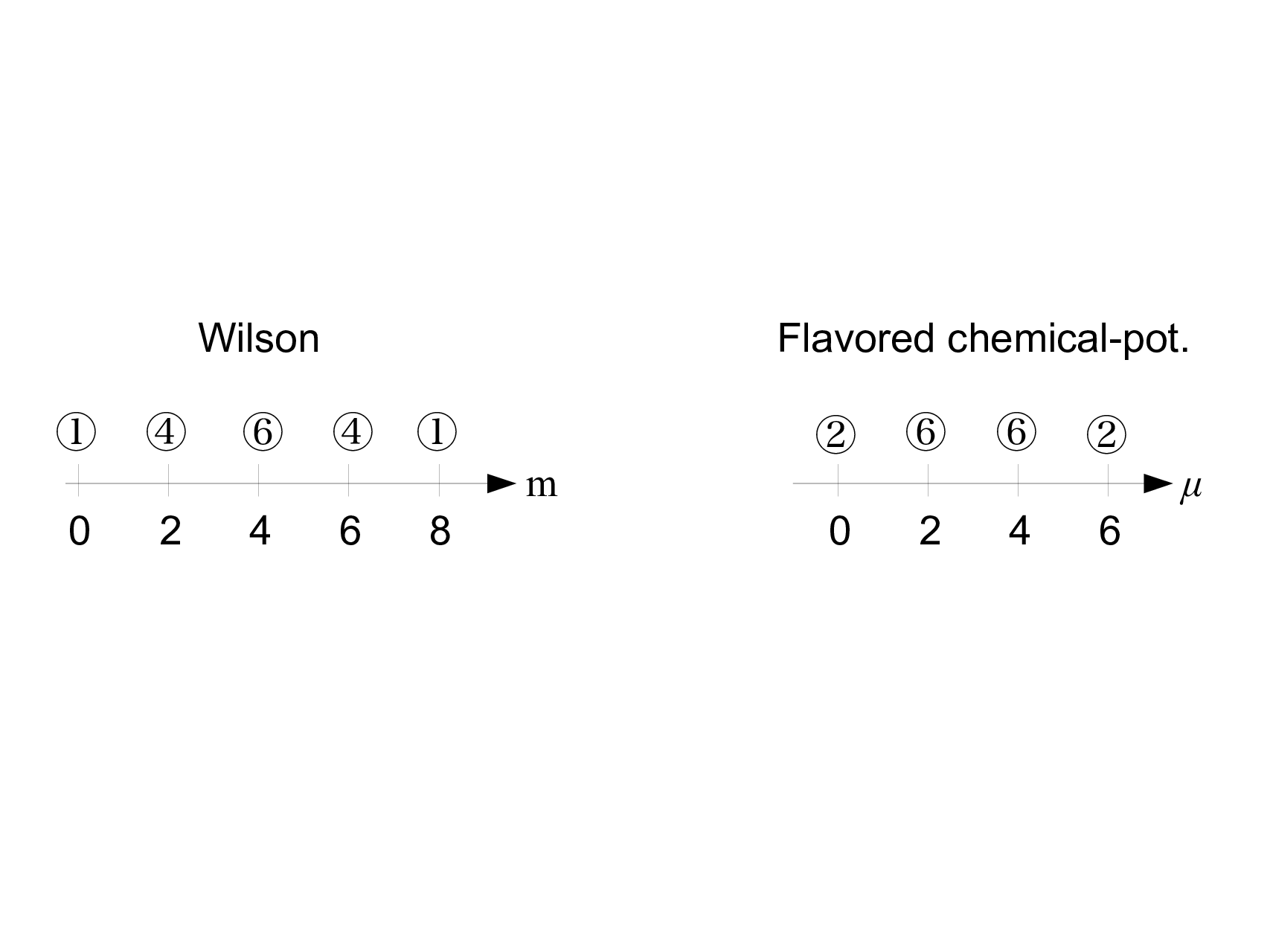
Here 14 species is decoupled in the naive continuum limit while two species at $p=(0,0,0,0)$ and $p=(0,0,0,\pi/a)$ has zero mass and zero imaginary chemical potential ¹¹ 1 These two species are not equivalent since the gamma matrices are differently defined between them as $\gamma_{\mu}^{\prime}=\Gamma^{-1}\gamma_{\mu}\Gamma$. In the above case it is given by $\Gamma=i\gamma_{4}\gamma_{5}$. This means the chiral symmetry possessed by this action is identified as a flavored one given by $\gamma_{5}\otimes\tau_{3}$.. More precisely, among 16 species, two species have zero imaginary chemical potential, six have $2/a$, six have $4/a$ and two have $6/a$. In Fig. 1 we compares specie-splitting of KW fermion in chemical potential space to that of Wilson fermion in mass space. It is notable that two-flavor is the minimal number allowed by the no-go theorem. This form has been known as the Karsten-Wilczek (KW) fermion [13, 14], which is the first known type of “minimal-doubling fermions” [13, 14, 15, 17, 16, 18]. It has one exact chiral symmetry, ultra-locality, cubic symmetry, CT and P.

Since the chemical potential term breaks discrete symmetries into the subgroup, we need to fine-tune three parameters for one dimension-3 ($\bar{\psi}i\gamma_{4}\psi$) and two dimension-4 ($\bar{\psi}\gamma_{4}\partial_{4}\psi$, $F_{j4}F_{j4}$) counterterms in order to take a Lorentz-symmetric continuum limit for the zero-($T$,$\mu$) lattice QCD simulations [24, 25, 26].

Among the three counterterms, in this paper we mainly deal with the dimension-3 term $\mu_{3}\bar{\psi}i\gamma_{4}\psi$ with a relevant parameter $\mu_{3}$ and the dimension-4 term $d_{4}\bar{\psi}\gamma_{4}\partial_{4}\psi$ with a marginal parameter $d_{4}$ since we study the strong-coupling lattice QCD and the Gross-Neveu model, which contain no plaquette action. In particular the parameter $\mu_{3}$ is of special importance: It changes the number of flavors and plays an important role in the chiral phase structure. Furthermore the quantum effects produce $O(1/a)$ additive chemical potential renormalization in this case instead the additive mass renormalization, and we need to cancel it by adjusting $\mu_{3}$ even for the application to the imaginary-chemical-potential lattice QCD. This necessity of parameter tuning is also understood from the well-known fact that the naive introduction of chemical potential into lattice fermions leads to divergence of energy density and requires a counterterm due to the violation of the abelian gauge invariance as shown in Ref. [37].

We here write the KW fermion action of the interacting theory as

	$\displaystyle S_{\mathrm{KW}}$	$\displaystyle=$	$\displaystyle\sum_{n}\Bigg[\frac{1}{2}\sum_{\mu=1}^{4}\bar{\psi}_{n}\gamma_{\mu}\left(U_{n,n+\mu}\psi_{n+\mu}-U_{n,n-\mu}\psi_{n-\mu}\right)$		(8)
			$\displaystyle+\frac{r}{2}\sum_{j=1}^{3}\bar{\psi}_{n}i\gamma_{4}\left(2\psi_{n}-U_{n,n+j}\psi_{n+j}-U_{n,n-j}\psi_{n-j}\right)+\mu_{3}\bar{\psi}_{n}i\gamma_{4}\psi_{n}+m\bar{\psi}_{n}\psi_{n}$
			$\displaystyle+{d_{4}\over{2}}\bar{\psi}_{x}\gamma_{4}\left(U_{n,n+4}\psi_{n+4}-U_{n,n-4}\psi_{n-4}\right)\Bigg],$

where we introduce a parameter $r$ in analogy with the Wilson parameter. We introduce the dimension-3 counterterm with the parameter $\mu_{3}$. Although we mainly focus on $\mu_{3}$ in this work, we also introduce the dimension-4 counterterm with the parameter $d_{4}$ in Eq. (8) which is also relevant for the strong-coupling study. We make all the quantities dimensionless. Now let us look into how the number of flavors depend on $\mu_{3}$. For a free theory, the associated massless Dirac operator in momentum space is

$$aD_{\mathrm{KW}}(p)=i\sum_{\mu=1}^{4}\gamma_{\mu}\sin ap_{\mu}+i\gamma_{4}(\mu_{3}+3r-r\sum_{j=1}^{3}\cos ap_{j}+d_{4}\sin ap_{4}).$$

(9)

We first look into a minimal-doubling range for $\mu_{3}$ and the speed of light in the range. We for simplicity take $r=1$. For $-1-d_{4}<\mu_{3}<1+d_{4}$, we have only two zeros, both of which have the form as $\bar{p}=(0,0,0,{1\over{a}}\arcsin(-{\mu_{3}\over{1+d_{4}}}))$. By expanding the momentum as $p=\bar{p}+q$ around the zeros, the coefficient of $i\gamma_{4}$ in the Dirac operator is given as

	$\displaystyle(1+d_{4})[\sin a\bar{p}_{4}\cdot\cos aq_{4}$	$\displaystyle+\cos a\bar{p}_{4}\cdot\sin aq_{4}]+\mu_{3}+3-\sum_{i=1}^{3}\cos(\bar{p}_{i}+q_{i})$
		$\displaystyle=[(1+d_{4})\cos a\bar{p}_{4}]\,aq_{4}+O(a^{2}q^{2}).$		(10)

Therefore, for general values of $\mu_{3}$ in this range, the speed of light is modified as

$$\sim q_{4}(1+d_{4})\sqrt{1-{\mu_{3}^{2}\over{(1+d_{4})^{2}}}}+O(aq^{2}).$$

(11)

We can fix this speed of light to a correct value up to the $O(a)$ discretization errors by taking $(1+d_{4})^{2}=1+\mu_{3}^{2}$. We will discuss details of Lorentz symmetry restoration in Sec.V. Now, let us classify $\mu_{3}$ parameter regions by the number of physical flavors in the free theory. Since $d_{4}$ just gives a shift of the parameter regions, we now consider $d_{4}=0$ for simplicity. The above minimal-doubling range is given just by $-1<\mu_{3}<1$. For $-7<\mu_{3}<-5$, we again have two zeros. For $\mu_{3}<-7$ and $\mu_{3}>1$, there is no zero of the Dirac operator, which means that there are no physical fermions. For $-5<\mu_{3}<-3$ and $-3<\mu_{3}<-1$, six zeros exist. $\mu_{3}=1,-7$ have one zero, but the dispersion relations have a unphysical form as $\sim{\bf p}+p_{4}^{2}$. $\mu_{3}=-1,-5$ have four zeros, but the dispersions are unphysical. $\mu_{3}=-3$ has six zeros, but the dispersion is again unphysical. In the end, the parameter ranges where physical fermions can be described are $-7<\mu_{3}<-5$ (2 flavors), $-5<\mu_{3}<-3$ (6 flavors), $-3<\mu_{3}<-1$ (6 flavors), $-1<\mu_{3}<1$ (2 flavors). We summarize it in Fig. 2. We note that nonzero $d_{4}$ gives larger minimal-doubling range as shown above.

What we want to study in this work is how these parameter ranges evolve in the finite gauge coupling direction. The most important question for practical use of this formulation in lattice QCD is how the two-flavor range, or the minimal-doubling range changes in the interacting theory. Our question is deeply related to a possible chiral phase structure with respect to the $U(1)$ chiral symmetry. It is because spontaneous chiral symmetry breaking is expected to occur only in parameter ranges with physical fermions. We thus speculate that boundaries between $\chi$SSB and non-$\chi$SSB phases starts from $\mu_{3}=-7$ and $\mu_{3}=1$ in the weak-coupling limit. From next section, we will elucidate the $\mu_{3}$-$g^{2}$ chiral phase diagram by using strong-coupling lattice QCD and the Gross-Neveu model.

In this section we employ the strong coupling analysis to investigate the chiral phase structure in lattice QCD with Karsten-Wilczek (KW) fermion. The first step is to derive an effective potential of meson fields corresponding to the fermion action in Eq. (8). The strong-coupling study for KW fermion was first performed by the present author and collaborators in [38]. We here take the same approach.

Lattice fermion action is generally written as following by using hopping operators $P^{\pm}_{\mu}$ and an onsite operator $\hat{M}$

$$S=\sum_{n,\mu}\bar{\psi}_{n}(P_{\mu}^{+}\psi_{n+\mu}-P_{\mu}^{-}\psi_{n-\mu})+\sum_{n}\bar{\psi}_{n}\hat{M}\psi_{n}.$$

(12)

By using these operators an effective action for mesons in the strong coupling limit can be written [8] as

	$\displaystyle S_{\rm eff}(\mathcal{M})$	$\displaystyle=$	$\displaystyle N_{c}\sum_{n}\left[\sum_{\mu}{\rm Tr}\,f(\Lambda_{n,\mu})+{\rm tr}\,\hat{M}\mathcal{M}(n)-\rm{tr}\,\,\log\mathcal{M}(n)\right]\,,$		(13)
	$\displaystyle\Lambda_{n,\mu}$	$\displaystyle=$	$\displaystyle\frac{V_{n,\mu}\bar{V}_{n,\mu}}{N^{2}_{c}},\quad\mathcal{M}(n)^{\alpha\beta}=\frac{\sum_{a}\bar{\psi}_{n}^{a,\alpha}\psi_{n}^{a,\beta}}{N_{c}}\,,$

	$\displaystyle V_{n,\mu}^{ab}$	$\displaystyle=$	$\displaystyle\bar{\psi}_{n}^{b}P^{-}_{\mu}\psi_{n+\hat{\mu}}^{a}\,,\quad\bar{V}_{n,\mu}^{ab}=-\bar{\psi}_{n+\hat{\mu}}^{b}P^{+}_{\mu}\psi_{n}^{a}\,,\quad$		(14)
	$\displaystyle{\rm Tr}\,f(\Lambda_{n,\mu})$	$\displaystyle=$	$\displaystyle-{\rm tr}\,f\left(-\mathcal{M}(n)(P^{+}_{\mu})^{\mathrm{T}}\mathcal{M}(n+\hat{\mu})(P^{-}_{\mu})^{\mathrm{T}}\right)\,,$		(15)

where $N_{c}$ is the number of colors, ${\rm Tr}$ ( $\rm{tr}\,$ ) means a trace over color(spinor) index, and $\mathcal{M}(n)$ is a meson field. $a,b$ are indices for colors while $\alpha,\beta$ for spinors. The explicit form of the function $f$ is determined by performing a one-link integral of the gauge field. In the large $N_{c}$ limit, it is known that $f(x)$ can be analytically evaluated [10] as

$$f(x)=\sqrt{1+4x}-1-\ln\frac{1+\sqrt{1+4x}}{2}=x+O(x^{2})\,.$$

(16)

For most cases of studying phase structure, we can approximate it as $f(x)\sim x$, which corresponds to a large-dimension limit [39]. Since the phase transition is expected to be second-order for a massless case, this approximation at least works well near the phase boundary. We however note that it becomes less valid for large $\sigma$. In the case of the Karsten-Wilczek fermion, we have $\hat{M}=m{\bf 1}_{4}+\mathrm{i}(\mu_{3}+3r)\gamma^{\mathrm{T}}_{4}$ and

$\displaystyle P^{+}_{\mu}$

$\displaystyle=$

$\displaystyle\left\{\begin{array}[]{ccc}\frac{1}{2}(\gamma_{\mu}+ir\gamma_{4})&\mu=1,2,3\\ \frac{1}{2}\gamma_{4}(1+d_{4})&\mu=4\\ \end{array}\right.,\quad P^{-}_{\mu}=\left\{\begin{array}[]{ccc}\frac{1}{2}(\gamma_{\mu}-ir\gamma_{4})&\mu=1,2,3\\ \frac{1}{2}\gamma_{4}(1+d_{4})&\mu=4\\ \end{array}\right..$

We here assume a form of meson condensate with chiral and 4th vector condensates as

$$\mathcal{M}_{0}=\sigma{\bf 1}_{4}+i\pi_{4}\gamma_{4}.$$

(22)

It is because the flavored chemical potential term is expected to produce 4th vector condensate, which is related to quark density. (We will discuss possibility of other condensates in the end of this section.) The explicit form of the effective action for $\sigma$ and $\pi_{4}$ is given by

	$\displaystyle S_{\rm eff}$	$\displaystyle=-4N_{c}{\rm Vol.}\mathcal{V}_{\rm eff}(\sigma,\pi_{4}),$		(23)
	$\displaystyle\mathcal{V}_{\rm eff}(\sigma,\pi_{4})$	$\displaystyle={1\over{2}}\log(\sigma^{2}+\pi_{4}^{2})-m\sigma+(\mu_{3}+3r)\pi_{4}$
		$\displaystyle\,\,\,\,\,\,\,-{1\over{4}}[3(1+r^{2})+(1+d_{4})^{2}]\sigma^{2}-{1\over{4}}[3(1-r^{2})-(1+d_{4})^{2}]\pi_{4}^{2}.$		(24)

We now find saddle points of $S_{\rm eff}(\mathcal{M})$ from

$\displaystyle{\delta S_{\rm eff}\over{\delta\sigma}}={\delta S_{\rm eff}\over{\delta\pi_{4}}}=0.$

(25)

Then gap equations are given by

	$\displaystyle\frac{3(1+r^{2})+(1+d_{4})^{2}}{2}\sigma+m-\frac{\sigma}{\sigma^{2}+\pi_{4}^{2}}$	$\displaystyle=$	$\displaystyle 0\,,$		(26)
	$\displaystyle\frac{3(1-r^{2})-(1+d_{4})^{2}}{2}\pi_{4}-(\mu_{3}+3r)-\frac{\pi_{4}}{\sigma^{2}+\pi_{4}^{2}}$	$\displaystyle=$	$\displaystyle 0\,.$		(27)

It is notable that these gap equations have a particle-hole symmetry as $(\pi_{4},\mu_{3}+3)\leftrightarrow(-\pi_{4},-\mu_{3}-3)$, which is reflected by chiral phase structure as we will see later. We first consider $m=0$, and solve the equations analytically. One of the main purposes here is to find a boundary between chiral symmetric and broken phases. For this purpose we take $\sigma=0$ after dividing the first equation by $\sigma$ since $\sigma$ is an order parameter of chiral symmetry breaking. Then we have

		$\displaystyle{3(1+r^{2})+(1+d_{4})^{2}\over{2}}=\frac{1}{\pi_{4}^{2}}\,,$		(28)
		$\displaystyle{3(1-r^{2})-(1+d_{4})^{2}\over{2}}\pi_{4}-(\mu_{3}+3r)={1\over{\pi_{4}}}\,.$		(29)

These equations give chiral boundaries for $\mu_{3}$ as

$$\mu_{3}=\pm{6r^{2}+2(1+d_{4})^{2}\over{\sqrt{6r^{2}+2(1+d_{4})^{2}+6}}}-3r.$$

(30)

Therefore we have two ranges of $\mu_{3}$ with different chiral properties, I and II :

		$\displaystyle{\rm{\bf I}}\,:\,\,\,\,\,\,\,\,\,\,\mu_{3}<-{6r^{2}+2(1+d_{4})^{2}\over{\sqrt{6r^{2}+2(1+d_{4})^{2}+6}}}-3r,\,\,\,\,\,\,\,\,\,\,\mu_{3}>{6r^{2}+2(1+d_{4})^{2}\over{\sqrt{6r^{2}+2(1+d_{4})^{2}+6}}}-3r,$		(31)
		$\displaystyle{\rm{\bf II}}\,:\,\,\,\,\,\,\,\,\,\,-{6r^{2}+2(1+d_{4})^{2}\over{\sqrt{6r^{2}+2(1+d_{4})^{2}+6}}}-3r<\mu_{3}<{6r^{2}+2(1+d_{4})^{2}\over{\sqrt{6r^{2}+2(1+d_{4})^{2}+6}}}-3r.$		(32)

The question is which corresponds to the chiral symmetric or broken phases. We for a while look into the $r=1$ case to show details of chiral phase structure. Since the change of $d_{4}$ just shift the chiral phase boundary (30), we for a while take $d_{4}=0$ to catch the chiral phase structure although we note that we need to take care of it for a Lorentz symmetric continuum limit. For $r=1$ and $d_{4}=0$ the boundaries are given by $\bar{\mu}_{3}\equiv\mu_{3}+3=\pm\sqrt{32/7}$ ($\mu_{3}\sim-5.14,-0.86$). Here we defined shifted $\mu_{3}$ as $\bar{\mu}_{3}=\mu_{3}+3$. By solving the gap equations in Eq. (8)(27) for $r=1$ and $d_{4}=0$ we derive two solutions of chiral and $\pi_{4}$ condensates as

$$\mathcal{M}_{0}^{A}:\,\,\,\,\,\,\,\sigma=0,\,\,\,\,\pi_{4}=-\bar{\mu}_{3}+\sqrt{\bar{\mu}_{3}^{2}-2},$$

(33)

and

$$\mathcal{M}_{0}^{B}:\,\,\,\,\,\,\,\sigma={\sqrt{32-7\bar{\mu}_{3}^{2}}\over{4\sqrt{7}}},\,\,\,\pi_{4}=-{\bar{\mu}_{3}\over{4}}.$$

(34)

By comparing effective potentials of the two solutions, we find which corresponds to vacua for the two parameter ranges, I and II. We show the following by substituting the two solutions: $\mathcal{V}_{\mathrm{eff}}(\mathcal{M}_{0}^{A})-\mathcal{V}_{\mathrm{eff}}(\mathcal{M}_{0}^{B})>0$ for $-\sqrt{32/7}<\bar{\mu}_{3}<\sqrt{32/7}$ (II) while $\mathcal{V}_{\mathrm{eff}}(\mathcal{M}_{0}^{A})-\mathcal{V}_{\mathrm{eff}}(\mathcal{M}_{0}^{B})<0$ for $\bar{\mu}_{3}<-\sqrt{32/7},\,\,\bar{\mu}_{3}>\sqrt{32/7}$ (I). To sum up, the chiral symmetric and broken phases are given by

		$\displaystyle\sigma=0\,\,\,\,\,\,\,\,\,\,\,\,\,\,\,\,\,\,\,\,\,\,\,\,\,\,\,\,\,\,\,\,\,\,\,\,\,\,\,\,\,\,\,\,\,\,\,{\rm for}\,\,\,\,\,\,\mu_{3}<-\sqrt{32/7}-3,\,\,\mu_{3}>\sqrt{32/7}-3\,\,\,\,({\rm{\bf I}}),$		(35)
		$\displaystyle\sigma={\sqrt{32-7(\mu_{3}+3)^{2}}\over{4\sqrt{7}}}\,\,\,\,\,{\rm for}\,\,\,\,-\sqrt{32/7}-3<\mu_{3}<\sqrt{32/7}-3\,\,\,\,({\rm{\bf II}}).$		(36)

The behavior of chiral condensate is depicted as a function of $\bar{\mu}_{3}=\mu_{3}+3$ in Fig. 3, which shows that the transition between chiral symmetric and broken phases is second-order. We also depict parameter regions for the two phases in the strong-coupling limit for $r=1$, $d_{4}=0$ and $m=0$ in Fig. 4. As seen from Eq. (30), a nonzero $d_{4}$ gives a larger physical range (II) with SSB of chiral symmetry.

We show that the order of transition becomes a crossover for $m\not=0$. Fig.5 shows the chiral condensate as a function of $\bar{\mu}_{3}=\mu_{3}+3$ and $m$. It is obvious that the second-order phase transition changes into a crossover for $m\not=0$.

We note that $\pi_{4}$ condensate is in general non-zero in the chiral-broken phase. $\pi_{4}$ becomes zero only for $\mu_{3}+3=0$, which corresponds to a theory with unphysical dispersions.

We next look into mass of mesons within the same framework. We here consider $m=0$ but general values of $r$ and $d_{4}$. To calculate meson masses we expand the meson field as,

$$\mathcal{M}(n)=\mathcal{M}^{\mathrm{T}}_{0}+\sum_{X}\pi^{X}(n)\Gamma^{\mathrm{T}}_{X}\,,\quad X\in\left\{S,P,V_{\alpha},A_{\alpha},T_{\alpha\beta}\right\}\,,$$

(37)

where $S,P,V_{\alpha},A_{\alpha}$ and $T_{\alpha\beta}$ stand for scalar, pseudo-scalar, vector, axial-vector and tensor respectively. Here $\mathcal{M}_{0}$ is the vacuum expectation value of $\mathcal{M}(n)$. We note that

$\displaystyle\Gamma_{S}=\frac{{\bf 1}_{4}}{2},\ \Gamma_{P}=\frac{\gamma_{5}}{2},\ \Gamma_{V_{\alpha}}=\frac{\gamma_{\alpha}}{2},\ \Gamma_{A_{\alpha}}=\frac{i\gamma_{5}\gamma_{\alpha}}{2},\ \Gamma_{T_{\alpha\beta}}=\frac{\gamma_{\alpha}\gamma_{\beta}}{2i}\ (\alpha<\beta).$

(38)

Then the effective action at the second order of $\pi^{X}$ is given by

	$\displaystyle S_{\rm eff}^{(2)}$	$\displaystyle=$	$\displaystyle N_{c}\sum_{n}\biggl[\frac{1}{2}{\rm tr}\,(\mathcal{M}_{0}^{-1}\Gamma_{X}\mathcal{M}_{0}^{-1}\Gamma_{Y})\,\pi^{X}(n)\pi^{Y}(n)+\sum_{\mu}{\rm tr}\,(\Gamma_{X}P^{-}_{\mu}\Gamma_{Y}P^{+}_{\mu})\pi^{X}(n)\pi^{Y}(n+\hat{\mu})\biggr]$		(39)
		$\displaystyle=$	$\displaystyle N_{c}\int\frac{d^{4}p}{(2\pi)^{4}}\pi^{X}(-p)D_{XY}(p)\pi^{Y}(p)\,,$

where

	$\displaystyle D_{XY}(p)$	$\displaystyle=$	$\displaystyle\frac{1}{2}\bigl(\widetilde{D}_{XY}(p)+\widetilde{D}_{YX}(-p)\bigr),$		(40)
	$\displaystyle\widetilde{D}_{XY}(p)$	$\displaystyle=$	$\displaystyle\frac{1}{2}{\rm tr}\,(\mathcal{M}_{0}^{-1}\Gamma_{X}\mathcal{M}_{0}^{-1}\Gamma_{Y})+\sum_{\mu}{\rm tr}\,(\Gamma_{X}P^{-}_{\mu}\Gamma_{Y}P^{+}_{\mu})e^{ip_{\mu}}.$		(41)

In our case $\mathcal{M}_{0}=\sigma{\bf 1}+i\pi_{4}\gamma_{4}$ gives

$$\mathcal{M}_{0}^{-1}={1\over{\sigma^{2}+\pi_{4}^{2}}}(\sigma{\bf 1}-i\pi_{4}\gamma_{4}).$$

(42)

We now write the whole inverse meson propagator matrix in the $S$-$V$-$T$-$A$-$P$ sector as

		$\displaystyle D_{SVTAP}=$
		$\displaystyle\left[\begin{array}[]{cccccccccccccccc}D_{S}&-C&{-irs_{1}\over{2}}&{-irs_{2}\over{2}}&{-irs_{3}\over{2}}&&&&&&&&&&&\\ -C&D_{V_{4}}&&&&&&&&&&&&&&\\ {irs_{1}\over{2}}&&D_{T_{14}}&&&&&&&&&&&&&\\ {irs_{2}\over{2}}&&&D_{T_{24}}&&&&&&&&&&&&\\ {irs_{3}\over{2}}&&&&D_{T_{34}}&&&&&&&&&&&\\ &&&&&D_{V_{3}}&&&&&&{-irs_{2}\over{2}}&{irs_{1}\over{2}}&&&\\ &&&&&&D_{V_{2}}&&&&&{irs_{3}\over{2}}&&{-irs_{1}\over{2}}&&\\ &&&&&&&D_{V_{1}}&&&&&{-irs_{3}\over{2}}&{irs_{2}\over{2}}&&\\ &&&&&&&&D_{T_{12}}&&&&&C&{-irs_{3}\over{2}}&\\ &&&&&&&&&D_{T_{13}}&&&-C&&{irs_{2}\over{2}}&\\ &&&&&&&&&&D_{T_{23}}&C&&&{-irs_{1}\over{2}}&\\ &&&&&{irs_{2}\over{2}}&{-irs_{3}\over{2}}&&&&C&D_{A_{1}}&&&\\ &&&&&{-irs_{1}\over{2}}&&{irs_{3}\over{2}}&&-C&&&D_{A_{2}}&&\\ &&&&&&{irs_{1}\over{2}}&{-irs_{2}\over{2}}&C&&&&&D_{A_{3}}&\\ &&&&&&&&{irs_{3}\over{2}}&{-irs_{2}\over{2}}&{irs_{1}\over{2}}&&&&D_{P}&\\ &&&&&&&&&&&&&&&D_{A_{4}}\\ \end{array}\right]\,,$

where components are given by

	$\displaystyle D_{S}$	$\displaystyle={\sigma^{2}-\pi_{4}^{2}\over{2(\sigma^{2}+\pi_{4}^{2})^{2}}}+{1\over{4}}[(1+r^{2})(c_{1}+c_{2}+c_{3})+(1+d_{4})^{2}c_{4}],$		(60)
	$\displaystyle D_{V_{4}}$	$\displaystyle={\sigma^{2}-\pi_{4}^{2}\over{2(\sigma^{2}+\pi_{4}^{2})^{2}}}-{1\over{4}}[(1-r^{2})(c_{1}+c_{2}+c_{3})-(1+d_{4})^{2}c_{4}],$		(61)
	$\displaystyle D_{V_{3}}$	$\displaystyle={1\over{2(\sigma^{2}+\pi_{4}^{2})}}-{1\over{4}}[(1+r^{2})(c_{1}+c_{2})+(r^{2}-1)c_{3}+(1+d_{4})^{2}c_{4}],$		(62)
	$\displaystyle D_{V_{2}}$	$\displaystyle={1\over{2(\sigma^{2}+\pi_{4}^{2})}}-{1\over{4}}[(1+r^{2})(c_{1}+c_{3})+(r^{2}-1)c_{2}+(1+d_{4})^{2}c_{4}],$		(63)
	$\displaystyle D_{V_{1}}$	$\displaystyle={1\over{2(\sigma^{2}+\pi_{4}^{2})}}-{1\over{4}}[(1+r^{2})(c_{2}+c_{3})+(r^{2}-1)c_{1}+(1+d_{4})^{2}c_{4}],$		(64)
	$\displaystyle D_{T_{14}}$	$\displaystyle={1\over{2(\sigma^{2}+\pi_{4}^{2})}}-{1\over{4}}[(r^{2}-1)(c_{2}+c_{3})+(1+r^{2})c_{1}+(1+d_{4})^{2}c_{4}],$		(65)
	$\displaystyle D_{T_{24}}$	$\displaystyle={1\over{2(\sigma^{2}+\pi_{4}^{2})}}-{1\over{4}}[(r^{2}-1)(c_{1}+c_{3})+(1+r^{2})c_{2}+(1+d_{4})^{2}c_{4}],$		(66)
	$\displaystyle D_{T_{34}}$	$\displaystyle={1\over{2(\sigma^{2}+\pi_{4}^{2})}}-{1\over{4}}[(r^{2}-1)(c_{1}+c_{2})+(1+r^{2})c_{3}+(1+d_{4})^{2}c_{4}],$		(67)
	$\displaystyle D_{T_{12}}$	$\displaystyle={\sigma^{2}-\pi_{4}^{2}\over{2(\sigma^{2}+\pi_{4}^{2})^{2}}}+{1\over{4}}[(r^{2}-1)(c_{1}+c_{2})+(1+r^{2})c_{3}+(1+d_{4})^{2}c_{4}],$		(68)
	$\displaystyle D_{T_{13}}$	$\displaystyle={\sigma^{2}-\pi_{4}^{2}\over{2(\sigma^{2}+\pi_{4}^{2})^{2}}}+{1\over{4}}[(r^{2}-1)(c_{1}+c_{3})+(1+r^{2})c_{2}+(1+d_{4})^{2}c_{4}],$		(69)
	$\displaystyle D_{T_{23}}$	$\displaystyle={\sigma^{2}-\pi_{4}^{2}\over{2(\sigma^{2}+\pi_{4}^{2})^{2}}}+{1\over{4}}[(r^{2}-1)(c_{2}+c_{3})+(1+r^{2})c_{1}+(1+d_{4})^{2}c_{4}],$		(70)
	$\displaystyle D_{A_{1}}$	$\displaystyle={\sigma^{2}-\pi_{4}^{2}\over{2(\sigma^{2}+\pi_{4}^{2})^{2}}}+{1\over{4}}[(1+r^{2})(c_{2}+c_{3})+(r^{2}-1)c_{1}+(1+d_{4})^{2}c_{4}],$		(71)
	$\displaystyle D_{A_{2}}$	$\displaystyle={\sigma^{2}-\pi_{4}^{2}\over{2(\sigma^{2}+\pi_{4}^{2})^{2}}}+{1\over{4}}[(1+r^{2})(c_{1}+c_{3})+(r^{2}-1)c_{2}+(1+d_{4})^{2}c_{4}],$		(72)
	$\displaystyle D_{A_{3}}$	$\displaystyle={\sigma^{2}-\pi_{4}^{2}\over{2(\sigma^{2}+\pi_{4}^{2})^{2}}}+{1\over{4}}[(1+r^{2})(c_{1}+c_{2})+(r^{2}-1)c_{3}+(1+d_{4})^{2}c_{4}],$		(73)
	$\displaystyle D_{A_{4}}$	$\displaystyle={1\over{2(\sigma^{2}+\pi_{4}^{2})}}+{1\over{4}}[(1-r^{2})(c_{1}+c_{2}+c_{3})-(1+d_{4})^{2}c_{4}],$		(74)
	$\displaystyle D_{P}$	$\displaystyle={1\over{2(\sigma^{2}+\pi_{4}^{2})}}-{1\over{4}}[(1+r^{2})(c_{1}+c_{2}+c_{3})+(1+d_{4})^{2}c_{4}],$		(75)
	$\displaystyle C$	$\displaystyle={i\sigma\pi_{4}\over{(\sigma^{2}+\pi_{4}^{2})^{2}}},$		(76)

with $s_{k}=\sin p_{k}$ and $c_{k}=\cos p_{k}$. By diagonalizing this matrix, we can derive an explicit form of physical meson propagators. We note that $C$ gets zero in the chiral symmetric phase while it has nonzero values in the chiral broken phase.

We first check that pion mass becomes zero in the chiral-broken phase. For this purpose we substitute $p=(0,0,0,im_{P})$ into the propagator. Then $D_{P}$ is decoupled and the calculation gets simplified. We note that, in the chiral broken phase, the gap equation Eq. (8) gives $\sigma^{2}+\pi_{4}^{2}=2/[3(1+r^{2})+(1+d_{4})^{2}]$. Pion mass in the chiral broken phase with $r=1$ and $m=0$ is derived from a pole of $D_{P}$ with $p=(0,0,0,im_{P})$ as

	$\displaystyle D_{P}(0,0,0,im_{P})={3(1+r^{2})+(1+d_{4})^{2}\over{4}}-{1\over{4}}((1$	$\displaystyle+d_{4})^{2}\cos(im_{P})+3(1+r^{2}))=0$
		$\displaystyle\,\,\,\,\,\,\,\,\,\,\,\to\,\,\,\,\,\,\,\,\,\,\,\cosh(m_{P})=1.$		(77)

This mode corresponds to a massless NG boson associated with SSB of chiral $U(1)$ symmetry, which is consistent with realistic QCD.

On the second-order phase boundary, a divergent correlation length in the critical behavior should produce another massless mode. We here show that the scalar meson becomes massless on the critical line. An inverse meson propagator matrix in general has off-diagonal components, but substitution of $p=(0,0,0,im_{S})$ again decouples the scalar sector in the chiral-symmetric phase ($C=0$). An explicit form of the scalar inverse propagator is given by Eq. (60). Then we derive the scalar mass from a pole of this propagator with $p=(0,0,0,im_{S})$ as

$$D_{S}(0,0,0,im_{S})=0\,\,\,\,\,\to\,\,\,\,\cosh m_{S}=1-\Big[1+{3(1+r^{2})\over{(1+d_{4})^{2}}}+{1\over{(1+d_{4})^{2}}}{2(\sigma^{2}-\pi_{4}^{2})\over{(\sigma^{2}+\pi_{4}^{2})^{2}}}\Big].$$

(78)

As seen from this, scalar meson has nonzero mass in general. On the phase boundary, however, we have $\sigma=0$, $\pi_{4}=-\bar{\mu}_{3}+\sqrt{\bar{\mu}_{3}^{2}+2[3(1-r^{2})-(1+d_{4})^{2}]}$ and $\bar{\mu}_{3}=\pm{6r^{2}+2(1+d_{4})^{2}\over{\sqrt{6r^{2}+2(1+d_{4})^{2}+6}}}$ with $\bar{\mu}_{3}=\mu_{3}+3r$. It leads to zero $\sigma$ mass as

$$\cosh(m_{S})=1.$$

(79)

We can also show this from the chiral-broken phase. We have two massless modes only on the 2nd-order phase boundary, $\sigma$-meson and $\pi$-meson, which is inconsistent with the meson mass spectrum in QCD. We thus need to avoid this point in the simulation of QCD. In the first place this boundary corresponds to the boundary between the two-flavor and no-flavor ranges, which has the unphysical dispersion relation as shown in Sec. II. From the theoretical viewpoint, it is however an attractive topic. Further study including numerical simulations can elucidate detailed properties of this point.

References

- [1] L. H. Karsten and J. Smit, Nucl. Phys. B 183, 103 (1981).
- [2] H. B. Nielsen and M. Ninomiya, Nucl. Phys. B 185, 20 (1981); Nucl. Phys. B 193 173 (1981); Phys. Lett. B 105 219 (1981).
- [3] K. G. Wilson, Phys. Rev. D 10, 2445 (1974).
- [4] D. B. Kaplan, Phys. Lett. B 288, 342 (1992).
- [5] Y. Shamir, Nucl.Phys. B 406 90 (1993); V. Furman and Y. Shamir, Nucl. Phys. B 439, 54 (1995).
- [6] P. H. Ginsparg and K. G. Wilson, Phys. Rev. D 25, 2649 (1982).
- [7] N. Neuberger, Phys. Lett. B 427, 353 (1998).
- [8] J. B. Kogut and L. Susskind, Phys. Rev. D 11, 395 (1975).
- [9] L. Susskind, Phys. Rev. D 16, 3031 (1977).
- [10] N. Kawamoto and J. Smit, Nucl. Phys. B 192 (1981) 100.
- [11] H. S. Sharatchandra, H. J. Thun and P. Weisz, Nucl. Phys. B 192, 205 (1981).
- [12] M. F. L. Golterman and J. Smit, Nucl. Phys. B 245, 61 (1984).
- [13] L. H. Karsten, Phys. Lett. B 104, 315 (1981).
- [14] F. Wilczek, Phys. Rev. Lett. 59, 2397 (1987).
- [15] M. Creutz, JHEP 0804, 017 (2008) [arXiv:0712.1201 [hep-lat]].
- [16] A. Borici, Phys. Rev. D 78, 074504 (2008) [arXiv:0712.4401 [hep-lat]]; PoS LATTICE2008, (2008) [arXiv:0812.0092].
- [17] M. Creutz, PoS LATTICE2008, (2008) [arXiv:0808.0014].
- [18] M. Creutz and T. Misumi, Phys. Rev. D 82, 074502 (2010) [arXiv:1007.3328];
- [19] P. F. Bedaque, M. I. Buchoff, B. C. Tiburzi and A. Walker-Loud, Phys. Lett. B 662, 449 (2008) [arXiv:0801.3361 [hep-lat]]; M. I. Buchoff, PoS LATTICE2008 (2008) [arXiv:0809.3943].
- [20] P. F. Bedaque, M. I. Buchoff, B. C. Tiburzi and A. Walker-Loud, Phys. Rev. D 78, 017502 (2008) [arXiv:0804.1145 [hep-lat]].
- [21] T. Kimura and T. Misumi, Prog. Theor. Phys. 124, 415 (2010) [arXiv:0907.1371 [hep-lat]].
- [22] T. Kimura and T. Misumi, Prog. Theor. Phys. 123, 63 (2010) [arXiv:0907.3774 [hep-lat]].
- [23] K. Cichy, J. Gonzalez Lopez, K. Jansen, A. Kujawa and A. Shindler, Nucl. Phys. B 800, 94 (2008) [arXiv:0802.3637 [hep-lat]].
- [24] S. Capitani, J. Weber, H. Wittig, Phys. Lett. B 681, 105 (2009) [arXiv:0907.2825].
- [25] S. Capitani, J. Weber, H. Wittig, (2009) [arXiv:0910.2597].
- [26] S. Capitani, M. Creutz, J. Weber, H. Wittig, JHEP 1009, 027 (2010) [arXiv:1006.2009].
- [27] S. Aoki, Phys. Rev. D 30, 2653 (1984).
- [28] S. Aoki, Phys. Rev. D 33, 2377 (1986); 34, 3170 (1986); Phys. Rev. Lett. 57 3136 (1986); Nucl. Phys. B 314, 79 (1989).
- [29] S. Sharpe and R. Singleton, Phys. Rev. D 58, 074501 (1998).
- [30] M. Creutz, (1996) [arXiv:hep-lat/9608024].
- [31] V. Azcoiti, G. Di Carlo, A. Vaquero, Phys. Rev. D 79, 014509 (2009); S. Sharpe, Phys.Rev. D 79, 054503 (2009).
- [32] M. Creutz, T. Kimura and T. Misumi, JHEP 1012, 041 (2010) [arXiv:1011.0761].
- [33] B. Tiburzi, Phys. Rev. D 82 034511 (2010).
- [34] L. B. Drissi, E. H. Saidi, M. Bousmina, J. Math. Phys. 52 022306 (2010).
- [35] L. B. Drissi, E. H. Saidi, Phys. Rev. D 84 014509 (2011).
- [36] D. Chakrabarti, S. ands, A. Rago, JHEP 0906, 060 (2009).
- [37] P. Hasenfratz, F. Karsch, Phys. Lett. B 125, 308 (1983).
- [38] T. Kimura, S. Komatsu, T. Misumi, T. Noumi, S. Torii and S. Aoki, JHEP 1201, 048 (2012) [arXiv:1111.0402].
- [39] J. M. Blairon, R. Brout, F. Englert and J. Greensite, Nucl. Phys. B 180 439 (1981).
- [40] D. J. Gross and A. Neveu, Phys. Rev. D 10, 3235 (1974).
- [41] T. Eguchi and R. Nakayama, Phys. Lett. B 126, 89 (1983).
- [42] S. Aoki and K. Higashijima, Prog. Theor. Phys. 76, 521 (1986).
- [43] B. Leder, Ph.D. Thesis, [arXiv:0707.1939].
- [44] T. Korzec, Ph.D. Thesis, http://edoc.hu-berlin.de/docviews/abstract.php?id=28045 .
- [45] B. Leder, JHEP 0804, 044 (2008) [arXiv:0711.1072].
- [46] T. Izubuchi, J. Noaki and A. Ukawa, Phys. Rev. D 58, 114507 (1998) [arXiv:hep-lat/9805019].
- [47] T. Izubuchi and K. Nagai, Phys.Rev. D61, 094501 (2000) [arXiv:hep-lat/9906017].
- [48] M. Creutz, T. Kimura and T. Misumi, Phys. Rev. D 83, 094506 (2011) [arXiv:1101.4239].
- [49] S. Kamata, H. Tanaka, [arXiv:1111.4536] (2011).
- [50] H. Leutwyler, Phys. Rev. D 49, 3033 (1994).
- [51] T. Misumi, T. Kimura, A. Ohnishi, [arXiv:1206.1977] (2012).