Computing arithmetic Kleinian groupsThanks:
Aurel Page
Univ. Bordeaux, IMB, UMR 5251, F-33400 Talence, France.
CNRS, IMB, UMR 5251, F-33400 Talence, France.
INRIA, F-33400 Talence, France.
aurel.page@math.u-bordeaux1.fr
Abstract.
Arithmetic Kleinian groups are arithmetic lattices in . We present an algorithm that, given such a group , returns a fundamental domain and a finite presentation for with a computable isomorphism.
Introduction
An arithmetic Kleinian group is a discrete subgroup of with finite covolume that is commensurable with the image of the integral points of a form of defined over a number field under the natural surjection . Our main results are new deterministic and probabilistic algorithms for constructing fundamental domains for the action of arithmetic Kleinian groups on hyperbolic three-space that produce a finite presentation for . There is a substantial literature concerning such algorithms, some of which we review below. We compare our algorithms to recent ones and discuss numerical evidence suggesting that ours are more efficient. The algorithm presented here prepares the ground for computing the cohomology of these groups with the action of Hecke operators, which gives a concrete realization of certain automorphic forms by the Matsushima-Murakami formula [BW00]. By the Jacquet-Langlands correspondence [JL70], such forms are essentially the same as automorphic forms for over some number field. They should have attached Galois representations, but the construction of these representations in general is still an open problem. More generally, the integral (co)homology of such groups has recently received a lot of attention: for example the size of their torsion [BV13] and arithmetic functoriality [CV12] are being actively studied. Our algorithm allows for empirical study of these objects.
The problem of computing fundamental domains for such groups is well studied. In the analogous Fuchsian group case, i.e. a subgroup of , an algorithm may have been known to Klein and J. Voight [Voi09] has described and implemented an efficient algorithm exploiting reduction theory. In the special case of Bianchi groups, i.e. when the base field is imaginary quadratic and the group is split, R.G. Swan [Swa71] has described an algorithm, which was implemented by Riley [Ril83] and A. Rahm [Rah10]; D. Yasaki [Yas10] has described and implemented another algorithm based on Voronoï theory. C. Corrales, E. Jespers, G. Leal and Á. del Río [CJLdR04] have described an algorithm for the general Kleinian group case. They implemented it for one nonsplit group with imaginary quadratic base field. Our algorithm and implementation are more general, and experimentally more efficient in practice. We have recently found an unpublished algorithm of K. N. Jones and A. W. Reid, mentioned and briefly described in [CFJR01, section 3.1] that solves the same problem.
The article is organized as follows. In the first section we recall basic definitions and properties of hyperbolic geometry, quaternion algebras and Kleinian groups. In the second section we describe our algorithms: basic procedures to work in the hyperbolic -space, algorithms for computing a Dirichlet domain and a presentation with a computable isomorphism for a cocompact Kleinian group, and how to apply these algorithms to arithmetic Kleinian groups. In the third section we show examples produced by our implementation of these algorithms and comment on their running time.
I would like to thank John Voight for proposing me this project and supervising my master thesis, and Karim Belabas and Andreas Enge for their helpful comments on earlier versions of this article. Experiments presented in this paper were carried out using the PLAFRIM experimental testbed, being developed under the Inria PlaFRIM development action with support from LABRI and IMB and other entities: Conseil Régional d’Aquitaine, FeDER, Université de Bordeaux and CNRS (see https://plafrim.bordeaux.inria.fr/). This research was partially funded by ERC Starting Grant ANTICS 278537.
1. Arithmetic Kleinian groups
Here we recall basic definitions and properties of hyperbolic geometry, quaternion algebras and Kleinian groups. The general reference for this section is [MR03].
1.1. Hyperbolic geometry
The reader can find more about hyperbolic geometry in [Rat06]. The upper half-space is the Riemannian manifold with Riemannian metric given by
where , and . For , is the distance between and . The set is called the sphere at infinity. The upper half-space is a model of the hyperbolic -space, i.e. the unique connected, simply connected Riemannian manifold with constant sectional curvature . In this space, the volume of the ball of radius is .
The group acts on in the following way. Consider the ring of Hamiltonians with multiplication given by and for , and identify with the subset . Then for an element and , the formula
defines an action of on by orientation-preserving isometries. This action is transitive and the stabilizer of the point in is the subgroup .
The trace of an element of is defined up to sign, and we have the following classification of conjugacy classes in :
- •
If , then has two distinct fixed points in , no fixed point in and stabilizes the geodesic between its fixed points, called its axis. The element is conjugate to with ; it is called loxodromic.
- •
If , then has two distinct fixed points in , and fixes every point in the geodesic between these two fixed points. The element is conjugate to with ); it is called elliptic.
- •
If , then has one fixed point in and no fixed point in . It is conjugate to ; it is called parabolic.
1.2. The unit ball model
In actual computations we are going to work with another model of the hyperbolic -space. The unit ball is the open ball of center and radius in , equipped with the Riemannian metric
where , and . The sphere at infinity is the Euclidean sphere of center and radius . The distance between two points is given by the explicit formula
The upper half-space and the unit ball are isometric, the isometry being given by
and the corresponding action of an element on a point is given by
| (1) |
where
In the unit ball model, the geodesic planes are the intersections with of Euclidean spheres and Euclidean planes orthogonal to the sphere at infinity, and the geodesics are the intersections with of Euclidean circles and Euclidean straight lines orthogonal to the sphere at infinity. A half-space is an open connected subset of with boundary consisting of a geodesic plane. A convex polyhedron is the intersection of a set of half-spaces, such that the corresponding set of geodesic planes is locally finite.
1.3. The Lobachevsky function and volumes of tetrahedra
We are going to compute hyperbolic volumes, and for this the main tool is going to be the Lobachevsky function, which we define here. The integral
converges for and admits a continuous extension to that is odd and periodic with period . This extension is called the Lobachevsky function . The Lobachevsky function admits a power series expansion, converging for :
With this function we can derive a formula for the volume of a certain standard tetrahedron. We will use it to compute the volume of convex polyhedra.
Proposition 1.
Let be the tetrahedron in with one vertex at and the other vertices on the unit hemisphere projecting vertically onto in with to form a Euclidean triangle, with angles at and at , and such that the angle along is . Then the volume of is finite and given by
Proof.
This formula can be found in [MR03, paragraph 1.7]. ∎
1.4. Kleinian groups, Dirichlet domains and exterior domains
A subgroup of is a Kleinian group if it acts discontinuously on , or equivalently if it is a discrete subgroup of . A fundamental domain for is an open subset of such that
- (i)
;
- (ii)
For all ;
- (iii)
where is the Riemannian volume on . To compute a fundamental domain for a Kleinian group , we are going to use the standard construction of Dirichlet domains. Let be a point with trivial stabilizer in . Then the Dirichlet domain centered at
is a convex fundamental polyhedron for . If has finite covolume, then the closure of has finitely many faces. A Kleinian group is geometrically finite if the closure of one (equivalently, every) Dirichlet domain for has finitely many faces.
Note that since acts properly discontinuously on , every point outside a zero measure, closed subset of has a trivial stabilizer in . In the unit ball model, the Dirichlet domain centered at has a simple description. Consider an element not fixing . Let
- •
;
- •
;
- •
.
We call the isometric sphere of . For a subset such that no element of fixes , the exterior domain of is . The set is a defining set for . A minimal defining set for is a subset such that and for all , the geodesic plane contains a face of .
With these definitions it is clear that . Note that for all with trivial stabilizer in , where is such that , so there is no harm in restricting to the Dirichlet domain centered at . Consider an element and as in formula (1). Then if and only if and, if does not fix , then a simple but lengthy computation reveals that is the intersection of and the Euclidean sphere of center and radius , where
| (2) |
and that is the interior of this sphere. The details are in [Pag10, Proposition 3.1.6].
Another property of Dirichlet domains is their rich structure: it gives a presentation for the group, and also necessary and sufficient conditions for an exterior domain to be a fundamental fomain. Suppose is a Kleinian group in which has trivial stabilizer, and let . Then we have if and only if . We also have , and a point is in the defining set of if and only if is too.
From this, we can group the faces of in pairs, one contained in some and the other contained in , and send the faces to each other. This is the face pairing structure, and the elements such that contains a face of are called the face pairing transformations. They generate the group .
Now we are going to look for relations. The first type comes from edge cycles: consider an edge of contained in some , and let . We define inductively a sequence of edges and elements in in the following way. We let . Then is contained in for a unique (see Figure 1). If has finitely many faces, then the sequence is periodic, let be its period. The sequence of edges is a cycle of edges, and is its length. The cycle transformation at is , and has the property:
- (i)
The cycle transformation at fixes pointwise.
This implies that satisfies the cycle relation for some integer . If , the cycle is called elliptic. At every edge , the geodesic planes and make an angle inside . The cycle angle of is . Since the translates of cover a neighborhood of , we have the property:
- (ii)
The cycle angle is where is the order of the cycle transformation.
The second type of relations comes from elements of order : it may happen that , then the element satisfies the reflection relation .
1.5,2.55)(13.385,7.52),2.51)5.08.5752325141.3402 ,2.51)3.214.036243102.83561 4,2.51)1.238.65981109.53665 ,2.51)1.454.29331158.49857 ,2.51)0.660.25512142.43141 ,2.51)0.826.56505297.76517 31,-0.48)7.0395.41553125.0031 19,3.14)1.6126.87814172.87498 09,2.48)1.4971.21138144.75243
Theorem 2 (Poincaré).
Let be the Dirichlet domain of a geometrically finite Kleinian group . Then the face pairing transformation generate the group , and the reflection relations together with the cycle relations form a complete set of relations for .
Remark 3.
In the presentation given by the theorem we consider only one element for each pair of face-pairing transformation . If we take both in the set of generators, we have to add the “inverse” relation .
We are now looking for sufficient conditions for an exterior domain to be a fundamental domain. There is another necessary condition, coming from cycles of some special points at infinity. A point is a tangency vertex if it is a point of tangency of two faces of . If is a tangency vertex, then we define a sequence by letting while is a tangency vertex (otherwise the sequence ends at ). If such a sequence is infinite and has finitely many faces, then it is periodic. Let be its period; then is a tangency vertex cycle and the tangency vertex transformation is . The fact that is complete implies the property:
- (iii)
The tangency vertex transformation is parabolic.
Actually all these definitions can make sense for any exterior domain. Suppose is an exterior domain with a finite minimal defining set. We say that it has a face pairing if and for every the image by of the face contained in is the face contained in – equivalently, the image of every edge of by the pairing transformation of an adjacent face is an edge of . This implies that every cycle is well-defined. We say that it satisfies the cycle condition if every cycle satisfies the properties (i) and (ii), and that it is complete if every tangency vertex cycle satisfies the property (iii).
Theorem 4 (Poincaré).
Let be an exterior domain with finite. Suppose has a face pairing, satisfies the cycle condition, and is complete. Let be the group generated by the face pairing transformations. Then is a fundamental polyhedron for .
Proof.
Both theorems are a special case of the second Theorem in [Mas71]. ∎
1.5. Quaternion algebras and arithmetic Kleinian groups
We can now describe the construction of arithmetic Kleinian groups using orders in quaternion algebras. The reader can find more about quaternion algebra in [Vig80]. A quaternion algebra over a field is a central simple algebra of dimension over . Equivalently, if , there exists such that with multiplication table given by . Such an algebra is written . A quaternion algebra either is isomorphic to the matrix ring , or is a division algebra. Given an element , we define its conjugate , its reduced trace and its reduced norm .
Let be a number field, let be its ring of integers and let be a quaternion algebra over . An order is a finitely generated -submodule with that is also a subring. We write the subgroup of elements of reduced norm .
A place of is split or ramified depending on whether is isomorphic to the matrix ring or not. The set of ramified places is finite and the discriminant of is the product of the ramified finite places, viewed as an ideal in . The number field is almost totally real (or ATR) if it has exactly one complex place. A quaternion algebra over an ATR field is Kleinian if it is ramified at every real place.
Theorem 5.
Let be an ATR number field of degree , a Kleinian quaternion algebra over and be an order in . Let be an algebra homomorphism extending a complex embedding of . Then the group is a Kleinian group. It has finite covolume, and it is cocompact if and only if is a division algebra. Furthermore, if is maximal, we have
| (3) |
where is the discriminant of , is the Dedekind zeta function of , is the discriminant of and for every ideal of .
Proof.
This theorem can be found in [MR03, Theorems 8.2.2, 8.2.3 and 11.1.3]. ∎
An arithmetic Kleinian group is a Kleinian group that is commensurable with a group as in the previous theorem. This is equivalent to the definition given in the introduction. The object of the next section is to describe an algorithm that, given such a group, computes a fundamental domain for , and a presentation with a computable isomorphism.
2. Algorithms
We describe every algorithm in ideal arithmetic. In section 2.5, we explain how to implement these algorithms using floating-point arithmetic.
2.1. Algorithms for polyhedra in the hyperbolic -space
We start with low-level algorithms for dealing with hyperbolic polyhedra. A point in is represented by a vector in ; a geodesic plane not containing is represented by the Euclidean center and radius of the corresponding Euclidean sphere; a geodesic not containing is represented by the Euclidean center and radius of a Euclidean sphere and a basis of a Euclidean plane containing the center of the sphere, such that the geodesic is the intersection of , this sphere and this plane.
Using these representations, it is an exercise in computational geometry to see that we can compute the faces, edges and vertices of a convex polyhedron given by a finite set of half-spaces containing . The details can be found in [Pag10, section II.3.3]. A harder task is to compute the volume of such a polyhedron. We describe an algorithm here; it is essentially the same as the one described in [MR03, section 1.7] but for the sake of completeness we provide all the details here.
Algorithm 1 computes the volume of a convex polyhedron with finitely many faces.

Remarks 6.
- •
For step 1, choose a vertex of the face and link it to every other vertex;
- •
For step 2, choose a vertex of and link it to every computed triangle;
- •
- •
In step 6, the signs that appear in the sum are the signs of certain determinants;
- •
In step 8, the angle is an angle in a Euclidean triangle and can be computed by elementary trigonometry, and since the upper half-space model is conformal, the angle is the Euclidean angle of intersection of the sphere and plane representing the faces of the tetrahedron.
The values of the Lobachevsky function are computed with the following lemma. It may be well-known, but we include it for the sake of completeness.
Lemma 7.
For all we have the formula
and the bounds
Proof.
To derive the first expression we use the previous power series expansion and extract the first term of the series expansion of the zeta function. For all we have
since all these series converge. We only need to compute the power series that appears. By taking derivatives twice we find that for all we have
Letting in this expression gives the first formula.
To prove the inequalities we are going to bound the values and for . By series-integral comparison we get
giving
for the first value, and
for the second one. Using these inequalities and the bound , and computing the geometric sum gives the result. ∎
Remarks 8.
- •
With the same method, for any we can obtain a formula with remainder term .
- •
In practise, we precompute the coefficients of the power series we are using. By periodicity and oddness, we can always reduce to the case where : if the precision is fixed, we know a priori the maximal number of terms needed to evaluate the Lobachevsky function.
2.2. The reduction algorithm
When we have a fundamental domain, it is natural to ask for an algorithm that, given a point in the hyperbolic 3-space, computes an equivalent point in the fundamental domain and an element in the group that sends one point to the other.
Definition 9.
Let be a subset of a Kleinian group . A point is -reduced if for all , we have , i.e. if .
Proposition 10.
Given a finite subset of a Kleinian group and a point , Algorithm 2 returns a point and such that is -reduced and .
Proof.
After step 4, we have and . Because of the loop condition, while the algorithm runs the distance decreases. Since stays in the orbit of under and this orbit is discrete, the algorithm terminates. When it happens, is an element in such that is minimal and , so is -reduced. ∎
Remark 11.
At step 5, the achieving the minimal may not be unique. We can pick any of these elements. Ordering gives us a canonical choice.
Reducing points can give interesting information about the elements of the group, because if has a trivial stabilizer, then the orbit map is a bijection. This is the reason for introducing the following definition:
Definition 12.
Let be a subset of a Kleinian group and . An element is -reduced if is -reduced, i.e. if .
Given a finite , and , we can now compute an -reduced element such that as follows: we reduce with respect to ; if is such that is -reduced, then is -reduced. We also write the reduced element and simply . A priori this reduced element could depend on the chosen ordering in Algorithm 2.
Proposition 13.
Suppose that is a fundamental domain for . Then for outside of a zero measure, closed subset of , the following holds: for every , there exists a unique -reduced . If then if and only if .
Proof.
Let . The existence follows from Algorithm 2. For uniqueness, suppose and are -reduced and . Then , and since is in the orbit of , they are in fact in . Since these two points are in the same -orbit, we have . Now assume . If then , i.e. . If then and is -reduced so by uniqueness . Moreover the complement of in is a locally finite union of faces of , so it is closed with zero measure. ∎
Since this provides an algorithm to write an element of the group as a word in the generators and to compute modulo with explicit unique representatives, that particular kind of generating set deserves a name.
Definition 14.
A subset of a Kleinian group is a basis if is a fundamental domain for . If is also a minimal defining set for , it is called a normalized basis for .
2.3. Normalized basis algorithms
Now we describe a general algorithm that computes a normalized basis for a cocompact Kleinian group . We will then apply it to arithmetic groups. First note that, after conjugating the group by a suitable element in , we may assume that has a trivial stabilizer in and that every elliptic cycle has length .
We will use two blackbox subalgorithms, Enumerate and IsFullGroup:
- •
Enumerate() takes as an input a positive integer and returns a finite set of elements in (the integer is a parameter for iteration, it does not have any mathematical meaning);
- •
IsFullGroup() takes as an input a finite normalized basis for a subgroup and returns true or false according to whether or not.
In every algorithm, an exterior domain with finite is represented as a polyhedron in . We begin with a naive algorithm.
We say that Enumerate is a complete enumeration of if we have
Proposition 15.
If is geometrically finite and Enumerate is a complete enumeration of , then Algorithm 3 terminates after a finite number of steps and the output is a normalized basis for .
Proof.
The Dirichlet domain centered at for has finitely many faces by geometric finiteness. Since Enumerate is a complete enumeration, a defining set for this Dirichlet domain will be enumerated after a finite number of steps. The algorithm will then terminate as all the conditions are satisfied by Dirichlet domains. The output will then be a normalized basis for by Step 6 and Theorem 4. ∎
We will now use the reduction algorithm to improve upon Algorithm 3. The main ideas are
- •
reducing the elements that we have to find smaller ones
- •
when the face-pairing condition, the cycle condition or the completeness condition fails, using this fact to find elements that make the exterior domain smaller.
For clarity, we divide Algorithm 4 into four routines. Algorithm 4 uses these routines to compute a normalized basis for a geometrically finite Kleinian group .
The first routine, KeepSameGroup, reduces elements as much as possible to eliminate redundant ones and find smaller ones.
Proposition 16.
If is a subset of a Kleinian group, then Algorithm 5 terminates and does not change the group generated by .
Proof.
We first prove the second claim. Every element added to belongs to the group generated by as it is a reduction by of an element in . Moreover, every element that is discarded has so at the end of the loop we have , and every other element is replaced by , so the group generated by does not change.
Now we prove that the algorithm terminates. First consider the initial . Let and . The set is finite since is a Kleinian group, and we have . By definition of reduction, every element added to is in . Moreover, by Step 2 if an element is discarded then its isometric sphere does not intersect , so is in the complement of : cannot be the reduction of any element, so it cannot be added again. Similarly if is replaced by , then is not reduced so it cannot be added again. Hence the algorithm terminates. ∎
The second routine, CheckPairing, checks whether has a face-pairing. If it does not, it finds elements that make smaller.
Proposition 17.
If does not have a face-pairing, then after applying Algorithm 6, is strictly smaller.
Proof.
If there is a nonpaired edge, at Step 5, since we have and since we have . Putting these two together gives , i.e. so finally we have . ∎
We give a second possible algorithm for CheckPairing. It is simpler but less efficient in practice. It uses the fact that if a non-elliptic cycle has length three (which is generically the case), then it is of the form , , .
Proposition 18.
If does not have a face-pairing, then after applying Algorithm 7, is strictly smaller.
Proof.
If there is a nonpaired edge, then there exists elements in the minimal defining set of and a point such that (so that ). Since we also have and is not contained in , we get , so these elements will be considered in the loop. On the other hand we have , so : we have . ∎
Remark 19.
Although this algorithm is less efficient than Algorithm 6, it is interesting as it gives a geometric understanding of the method described in [Lip02]: “we consider words that are two-word combinations of those forming the sides of the existing domain to modify the domain. (…) This procedure has proven to be fast and effective in practice.” Proposition 18 explains why taking products of two elements forming the sides of the domain is useful, and in Algorithm 7 we get a geometric description of the the products that we should form. Actually, the computation in the proof of Proposition 7 also shows that if reduces , then .
The third routine, CheckCycleCondition, checks whether satisfies the cycle condition. If it does not, it finds elements that make smaller.
Remarks 20.
- •
- •
- •
Assuming both, we can omit CheckCycleCondition completely.
Lemma 21.
Suppose is a subset of a Kleinian group such that has a trivial stabilizer in , and suppose there is an element and a point such that . Then .
Proof.
First suppose that . Then writing we get i.e. . Since we also have , we obtain .
Othewise we have . This means that , but since we get . ∎
Proposition 22.
If does not satisfy the cycle condition, then after applying Algorithm 8, is strictly smaller.
Proof.
Since the cycle transformation at an edge stabilizes it, if the edge is not equal to a geodesic then the cycle transformation fixes it pointwise and condition (i) is automatically satisfied. Suppose that there is a cycle for an edge equal to a geodesic and that does not satisfy condition (i), and let be the corresponding cycle transformation. Then the transformation is either loxodromic, or elliptic of order with exactly one fixed point in . In both cases, Step 4 is executed. In the first case, since the interior of the isometric sphere of a loxodromic element contains one of its fixed points and the interior of the isometric sphere of its inverse contains the other, we have so . In the second case, the edge contains exactly one fixed point of in , so we again have and we get .
Now suppose some cycle angle for a non-elliptic cycle is larger than . Then considering the images of that glue one after another around , we see that there is an overlap: there exists a point such that for some considered in Step 10. In this case after Step 11 we have by Lemma 21. Since the cycle transformation is the identity, the angle cannot be smaller than .
Finally suppose some cycle angle for an elliptic cycle at an edge with cycle transformation with order does not satisfy condition (ii). The cycle has length , so , and the angle at is a multiple of . After running Step 6 the domain is replaced by the Dirichlet domain of the finite group , which satisfies the cycle condition, so the new angle at is equal to . ∎
The fourth routine, CheckComplete, checks whether is complete. If it is not, it finds elements that make smaller.
Remark 23.
If we know in advance that the group is cocompact, we can omit CheckComplete in Algorithm 4 and simply test whether is bounded.
Proposition 24.
If is not complete, then after applying Algorithm 8, is strictly smaller.
Proof.
If is a tangency vertex transformation at , then it fixes . By looking at the successive images of the polyhedron along the cycle we see that separates from , so has infinite order. If is not complete, then is loxodromic. Being a fixed point of , the point is contained in , so we get . ∎
Proposition 25.
Let be a Kleinian group. The following holds for Algorithm 4 applied to :
- (i)
Suppose the algorithm terminates. Then the output is a normalized basis for .
- (ii)
Suppose that is geometrically finite and Enumerate is a complete enumeration of . Then the algorithm terminates.
Remark 26.
In practise Algorithm 4 runs much faster that the naive Algorithm 3 (see section 3.1.1), but unfortunately we could not prove it. What we believe is that in Algorithm 4 the blackbox Enumerate only needs to find a set of generators for the group, and then the other routines find the elements of the normalized basis; in Algorithm 3 the blackbox Enumerate needs to find directly the elements of the normalized basis, which is harder. The natural idea would be to put the routines in a loop that would not contain Enumerate in Algorithm 4, but then it is not clear whether this internal loop would terminate; actually in general it is false, since may admit finitely generated subgroups that are not geometrically finite.
Proof.
- (i)
If the algorithm terminates, then by Theorem 4, since is complete, has a face-pairing and satisfies the cycle condition, the set is a normalized basis for . It is then valid to use IsFullGroup to check that .
- (ii)
The closure of the Dirichlet domain centered at for has finitely many faces by geometric finiteness. Since Enumerate is a complete enumeration, a defining set for this Dirichlet domain will be enumerated after a finite number of steps. The algorithm will then terminate as all the conditions are satisfied by the Dirichlet domain.
∎
2.4. Instantiation of the blackboxes
2.4.1. Enumerate and IsFullGroup for a group given by generators
Suppose the group is given by a finite set of generators . We can take for Enumerate the algorithm that writes every word of length in the generators, and we can take for IsFullGroup the algorithm that reduces every element in with respect to the given normalized basis and returns whether every generator reduces to : by Proposition 13, this is equivalent to .
2.4.2. Enumerate and IsFullGroup for an arithmetic group
We provide a possible instantiation of the blackboxes Enumerate and IsFullGroup for an arithmetic group attached to a maximal order in a Kleinian quaternion algebra with base field of degree .
We describe IsFullGroup first. A subgroup is proper if and only if its covolume is infinite or at least twice the covolume of , the quotient of the covolumes being the index of the subgroup. Since comes from a maximal order, the covolume of is given by (3), which we can compute, and the covolume of a subgroup can be computed with Algorithm 1 once we have a normalized basis. We take for IsFullGroup the algorithm that computes the covolume by the formula and the volume of for the given normalized basis , and returns whether . Since is a normalized basis for , the polyhedron is a fundamental domain for so the volume equals the covolume of .
We now describe an instantiation of the blackbox Enumerate for the Kleinian group associated with an order in . Under the natural embedding , the order is discrete. Now suppose that we have a positive definite quadratic form . Then becomes a full lattice in a real vector space of dimension . We can use lattice enumeration algorithms such as the Kannan-Fincke-Pohst algorithm [FP85, Kan83] to enumerate elements in that are short with respect to . We can then select the elements having reduced norm . As we increase the bound on the values of , we will get every element in . A priori any such quadratic form would work, but here we describe one that has a geometric meaning.
Recall we can embed in in such a way that becomes discrete in . This embedding is only defined up to conjugation by an element of . Let be such an embedding. If we can take for example
where is a complex embedding of , and is a square root of .
For , we define .
Proposition 27.
The quadratic form defined by
is positive definite and satisfies
where denotes the Euclidean radius of the isometric sphere of if , and otherwise.
Proof.
We show first that is positive definite. For a matrix we have where is the usual norm on , so that is a positive definite quadratic form on . Since is a positive definite quadratic form on and we have the decomposition , we can construct a positive definite quadratic form on by letting for all
where
since . This gives the positive definiteness.
We obtain the following enumeration algorithm. It is a complete enumeration of , and depends on a parameter: a sequence of bounds .
We are now going to present a probabilistic enumeration algorithm. It is not a complete enumeration, but performs better in pratice (see section 3.1.2). It uses variants of the former quadratic form.
Definition 28.
Let . Let be such that and . We then define the quadratic form by
for all .
This family of quadratic forms has the following properties.
Proposition 29.
Let . Then does not depend on the choice of such that and . It is positive definite, and for all we have
Proof.
The matrices and are defined up to right multiplication by , the stabilizer of the point . For all matrices we have , which is not changed by left and right multiplication of by elements of , so that does not depend on the choice of and .
For the formula reads for all , which is well-known (and is a direct consequence of the explicit formulas for the hyperbolic distance). Then for arbitrary we have
∎
This family of quadratic forms is very useful, as it enables us to determine the elements such that is close to . We propose the following probabilistic algorithm for enumerating elements in . It depends on a choice of some parameters: an increasing sequence of positive numbers representing the radius of the search space, a sequence of positive integers representing the number of enumerations in small balls, and a positive number being a bound on the quadratic form. For , we write .
Remarks 30.
- •
We can also use these quadratic forms differently: if we miss an element of the group to “close off” the exterior domain around a point at infinity , we can look for elements of small where . This is a similar idea as in Remark 4.9 in [Voi09], but the quadratic form that was used there is the analogue of . If is the element that we are looking for, is bounded by below by a positive constant if is loxodromic, which is the generic case. On the contrary we have as .
- •
The efficiency of this algorithm depends on the choice of the parameters , and . Heuristics led us to the following choice, which works well in practise:
- –
we use a small bound so that the number of such that is approximately constant by Gaussian heuristic;
- –
experimental evidence and [BGLS10, Theorem 1.5] suggest that a number of random elements of proportional to has a good probability to generate , and by Gaussian heuristic we need random centers to obtain one element of the group on average, so we choose , and we increase it exponentially fast: ;
- –
the radius has to be large enough to ensure good randomness of the elements of , so we choose such that and we increase it in arithmetic progression (so the volume increases exponentially fast): . Because of our choice of we take .
- –
Now we explain how we draw points at random in the ball of radius . Since the hyperbolic volume is invariant by rotation around , it is equivalent to draw a random point uniformly on the sphere, and then multiply it by an appropriate random scalar independent from the point on the sphere. Thus we only have to determine the distribution of the distance from of the points in the ball of radius . Let be a random variable with uniform distribution in . The cumulative distribution function of the distance to is
Recall that the volume of the ball of radius is . It is clear that the function is a continuous bijection. It implies that where is a uniform random variable in . We rewrite that expression as where is a uniform variable in . It is well-known how to draw a uniform variable in an interval and on a sphere, and can be computed by Newton iteration.
2.5. Floating-point implementation
Here we describe a floating-point implementation of the above algorithms. We start with a lemma giving us control on the error made when having an element of the group act on a point. We only study the stability of the algorithm, so we do not take into account the error made by rounding in elementary operations.
Lemma 31.
Let , and . Let , and . Suppose that . Then the quantity obtained by applying Formula (1) to and is well-defined, and we have
Proof.
By direct computation we have and , and the same inequalities for . We write
and similarly for . Another direct computation gives
| (4) |
showing that
By the triangle inequality, adding and substracting gives
and the same inequality for . We get
since by hypothesis we have . In particular and is well-defined. By the mean value theorem this gives
We also get
Finally we have
as claimed. ∎
In the following, we want to maintain the property for every element and every point considered, where is the imprecision on the points in , the imprecision on the elements considered, and .
We now describe the modification of the algorithms for the floating-point version. In the reduction algorithm (Algorithm 2), we choose and in Step 6 we replace the inequality by . Since we have if and only if , the modified condition is indeed an approximation of the exact condition.
Proposition 32.
Let where and . If , then the floating-point version of the reduction algorithm terminates.
Proof.
We want to use a uniform that tends to as . For this, we assume that we only consider points such that and elements such that . Assuming that we can then take . These assumptions also ensure that , and are compatible since the points that we have to consider satisfy .
There is no change in KeepSameGroup (Algorithm 5): the same argument shows that the algorithm terminates, regardless of finite precision in the computations.
The routine CheckPairing (Algorithm 6) should only consider an edge contained in as not being paired if there is and we have the stronger inequality and correspond to for some . This ensures that the floating-point reduction will yield a non-trivial element, since at least one step of reduction will be performed.
The routines CheckCycleCondition (Algorithm 8) and CheckComplete (Algorithm 9) contain only finite loops regardless of the use of finite precision, so there is no change in them.
Proposition 33.
The floating-point version of the Normalized basis algorithm (Algorithm 4) terminates.
Proof.
By the arguments above, each of the routines terminates. Moreover, because of precision restriction we impose for every element of the group considered in the algorithm, so that only finitely many can be used, so the algorithm terminates. ∎
Of course if the precision chosen is insufficient, the algorithm may terminate with an error or a wrong answer, but with Riley’s methods [Ril83], we can use Poincaré’s theorem with the approximate fundamental domain to prove that the computed presentation is correct. Alternatively, we could check the fundamental domain algebraically, but this is likely to be time-consuming.
2.6. Master algorithm
As a summary, this is our master algorithm for computing an arithmetic Kleinian group associated with a maximal order.
Remarks 34.
- •
If we want to compute the group that is the image of a smaller order, or more generally a finite index subgroup of the group given by a maximal order , we can compute first a normalized basis for the larger group , and then compute the index by standard coset enumeration techniques. This gives the covolume of the smaller group, and even a set of generators for it, so we can then apply the same algorithm we described.
- •
We may also want to compute a maximal group in the commensurability class of . There are infinitely many conjugacy classes of such maximal groups, and they can be obtained as follow. Let be a maximal order in , and a finite set of primes of that split in . Let be an Eichler order of level where is the product of the primes in , and define to be the normalizer of in . Then every maximal group in the commensurability class of is conjugate to a group for some set and some maximal order , which can be taken from a set of representatives of the conjugacy classes of maximal orders in . Note however that some of the groups may not be maximal. Since each of these groups is the image in of the normalizer of an order in , we may use the same enumeration techniques. The index is given in terms of a class group and a finite quotient of units in , which can be computed, so again we get the covolume of this larger group, and can apply the same technique. The reader can refer to [Bor81] or [MR03, Section 11.4] for details on maximal groups.
3. Examples
The author has implemented the algorithm described in the previous section in the computer system Magma [BCP97]. Our package KleinianGroups is available at http://www.normalesup.org/~page/software.html. Here we show some examples of the output of this code. In sections 3.1 and 3.2, the computations are performed on a GHz Intel i7 processor with Magma v2.18-4. The more extensive computations of sections 3.3 and 3.4 are run on a GHz Intel Xeon E5420 processor from the PLAFRIM experimental testbed with Magma v2.17-12.
3.1. Comparison between subalgorithms
3.1.1. Comparison between the normalized basis algorithms
Consider the ATR sextic field of discriminant generated by an element such that , and let be its ring of integers. Let be the quaternion algebra ramified only at the real places of . Let be a maximal order in ; the choice does not matter as they are all conjugate. The Kleinian group has covolume . We compare our algorithm with the naive Algorithm 3. Both need a precomputation of seconds for the computation of the coefficients of the Lobachevsky power series and seconds for the evaluation of the Dedekind zeta function at . Our algorithm then computes a Dirichlet domain in seconds, and enumerates elements of , yielding elements of . The naive algorithm (actually we only removed the routine CheckPairing) computes the same Dirichlet domain in seconds and has to enumerate elements of , yielding elements of . The fundamental domain (Figure 3) has 18 faces and 42 edges.

3.1.2. Comparison between the enumeration algorithms
Consider the ATR number field of degree and discriminant , generated by an element such that , and let be its ring of integers. Let be the quaternion algebra ramified only at the real places of . Let be a maximal order in ; the choice does not matter as they are all conjugate. The Kleinian group has covolume . We compare the performance of our algorithm when using the enumeration algorithms 10 or 11. With the deterministic enumeration algorithm 10, our code computes a fundamental domain in hours and minutes ( seconds, most of which is enumeration), and enumerates vectors, yielding group elements. With the probabilistic enumeration algorithm 11, our code computes the same Dirichlet domain in seconds, and only needs to enumerate vectors, yielding group elements. It spends seconds for computing the value of the zeta function, seconds for enumeration, seconds for the routine KeepSameGroup, for CheckPairing and for computing the volume of the polyhedron. The fundamental domain (Figure 4) has faces and edges.

3.2. Relation to previous work
In this section we show how to recover examples covered by earlier work with our algorithm. When available, we provide a comparison of running times between public implementations and our code. The reader should keep in mind that these are only comparisons between implementations since the complexity of the algorithms is usually unknown.
3.2.1. Bianchi groups
Let be an imaginary quadratic field with ring of integers . Consider the quaternion algebra and the maximal order . Then the group is called a Bianchi group. There exists already several programs computing fundamental domains for these groups [Rah10, Yas10] but they only work for Bianchi groups while ours deals with general arithmetic Kleinian groups. Table 1 gives the running time (in seconds) of our Magma package and other public implementations. The first three columns correspond to the discriminant of the field, its class number and the covolume of . The last four columns display running times in seconds: Bianchi.gp [Rah10] written in GP [The11] implementing Swan’s algorithm for , our code KleinianGroups computing , the code provided by Magma implementing the algorithm of [Yas10] using Voronoï theory for , and our code for . Note that it is not surprising that computing is faster: the group is larger by an index , so the covolume is twice smaller and our computation is times shorter (see also section 3.4).
| volume | Bianchi | KG, | Magma | KG, | ||
|---|---|---|---|---|---|---|
| 1 | 0.169 | 0.015 | 0.93 | 0.43 | 0.83 | |
| 2 | 3.139 | 0.152 | 0.92 | 0.8 | 2.32 | |
| 3 | 6.449 | 0.176 | 1.22 | 1.11 | 2.06 | |
| 4 | 13.80 | 2.37 | 9.44 | 3.05 | 4.36 | |
| 5 | 19.43 | 3.83 | 19.9 | 5.33 | 6.96 | |
| 7 | 37.53 | 21.6 | 36.6 | 17.8 | 13.2 | |
| 6 | 44.72 | 25.7 | 45.1 | 17.3 | 16.4 | |
| 8 | 57.06 | 41.4 | 43.8 | 33.9 | 19.3 | |
| 10 | 82.93 | 7080. | 137. | 99.5 | 25.6 | |
| 11 | 132.3 | 1545. | 391. | 188. | 80.9 | |
| 9 | 148.5 | 3840. | 393. | 224. | 92.7 |
3.2.2. Arithmetic Fuchsian groups
Let be a totally real field and a quaternion algebra ramified at every infinite place but one. Let be an order in . Then the group embeds into , in which it is discrete with finite covolume: it is an arithmetic Fuchsian group. Using the action of on the upper half-plane J. Voight [Voi09] was able to compute fundamental domains for these groups. Since we have , a Fuchsian group can be seen as a Kleinian group leaving a geodesic plane stable. Using this we can also compute arithmetic Fuchsian groups with our code. Our probabilistic enumeration Algorithm 11 leads to an improvement in high degree. As an example, consider the totally real field with discriminant , generated by an element such that . Let with and . It is ramified at every real place but one. Let be a maximal order in . The Fuchsian group has coarea ; our code computes a fundamental domain for this group in minutes ( seconds). The code provided by Magma and implementing the algorithm of [Voi09] computes a fundamental domain for in hour and minutes ( seconds).
3.2.3. The Hamiltonians over
Consider the field and the quaternion division algebra . Then is a non-maximal order in . A fundamental domain for this group was computed by C. Corrales, E. Jespers, G. Leal and Á. del Río in [CJLdR04]. Using the method of Remark 34, our code can compute a fundamental domain for the group . It computes first a maximal order , and a fundamental domain for (having covolume ). By coset enumeration, it finds that has index in the larger group, and computes a fundamental domain for the initial group . The overall computation takes seconds.
3.3. A larger example
Consider the ATR field generated by an element such that , having discriminant . Let be the quaternion algebra where and . It is ramified exactly at the real places of . Let be a maximal order in . The group has covolume . Our code computes a fundamental domain for this group in hours and minutes ( seconds). It spends % of the time for enumeration, % for the routine KeepSameGroup, % for CheckPairing and % for computing the volume of the polyhedron. The fundamental domain has faces and edges.
3.4. Efficiency of the algorithm

According to geometers, the parameter encoding the complexity of an arithmetic Kleinian group is the covolume. In practise it is simpler to vary the discriminant of the base field (and hence the degree) and the norm of the discriminant of the quaternion algebra. It seems hard to estimate the running time of the algorithm in terms of these parameters. First, we do not know any bound on the radii of the isometric spheres containing the faces of the closure of the Dirichlet domain, or of generators of the group, so we do not know how many elements we have to enumerate. Then, even if we have generators of the group, we do not know how long the normalized basis algorithm could run before terminating (see also Remark 26).
We present numerical data obtained in a family. Since the running time increases very quickly with the discriminant of the field, we fixed the base field and varied the discriminant of the algebra. The field we chose is the ATR cubic field of discriminant . We computed groups for every algebra with discriminant less than , and one algebra every ten with discriminant less than .
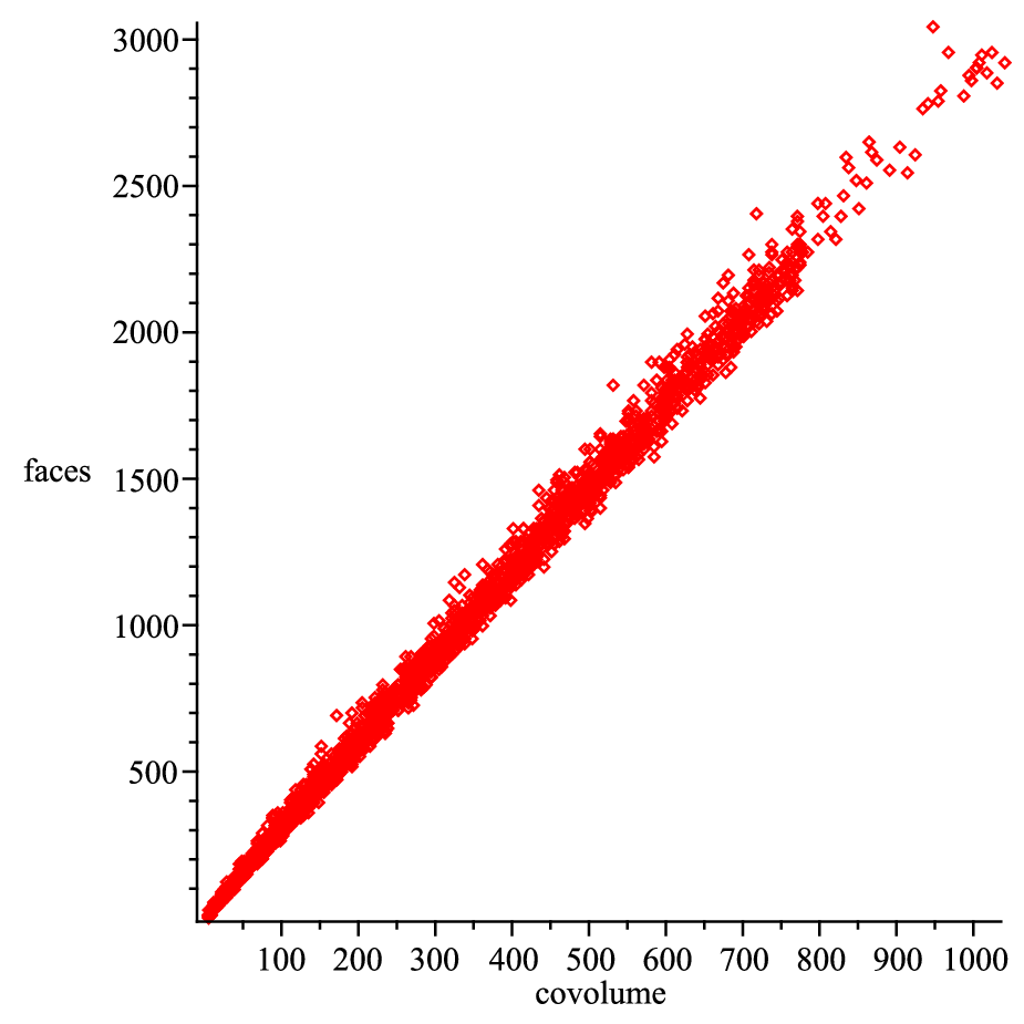
Analysis of this data shows that the running time is approximately proportional to the square of the covolume, with a few exceptionnally slow computations. We explain this as follows: in almost all cases, the enumeration appears to take negligible time, and the longest part is the computation of the fundamental domain itself; moreover the data (Figure 6) seem to indicate that the number of faces is proportional to the covolume (we have such a lower bound since the volume of a hyperbolic tetrahedron is bounded by ), and we know that our algorithm to compute the domain given the faces is quadratic.
References
- [BCP97] Wieb Bosma, John Cannon, and Catherine Playoust. The Magma algebra system. I. The user language. J. Symbolic Comput., 24(3-4):235–265, 1997. Computational algebra and number theory (London, 1993).
- [BGLS10] Mikhail Belolipetsky, Tsachik Gelander, Alexander Lubotzky, and Aner Shalev. Counting arithmetic lattices and surfaces. Ann. of Math. (2), 172(3):2197–2221, 2010.
- [Bor81] A. Borel. Commensurability classes and volumes of hyperbolic -manifolds. Ann. Scuola Norm. Sup. Pisa Cl. Sci. (4), 8(1):1–33, 1981.
- [BV13] Nicolas Bergeron and Akshay Venkatesh. The asymptotic growth of torsion homology for arithmetic groups. J. Inst. Math. Jussieu, 12(2):391–447, 2013.
- [BW00] A. Borel and N. Wallach. Continuous cohomology, discrete subgroups, and representations of reductive groups, volume 67 of Mathematical Surveys and Monographs. American Mathematical Society, Providence, RI, second edition, 2000.
- [CFJR01] Ted Chinburg, Eduardo Friedman, Kerry N. Jones, and Alan W. Reid. The arithmetic hyperbolic 3-manifold of smallest volume. Ann. Scuola Norm. Sup. Pisa Cl. Sci. (4), 30(1):1–40, 2001.
- [CJLdR04] Capi Corrales, Eric Jespers, Guilherme Leal, and Angel del Río. Presentations of the unit group of an order in a non-split quaternion algebra. Adv. Math., 186(2):498–524, 2004.
- [CV12] Frank Calegary and Akshay Venkatesh. A torsion Jacquet–Langlands correspondence. 2012. http://arxiv.org/abs/1212.3847.
- [FP85] U. Fincke and M. Pohst. Improved methods for calculating vectors of short length in a lattice, including a complexity analysis. Math. Comp., 44(170):463–471, 1985.
- [JL70] H. Jacquet and R. P. Langlands. Automorphic forms on . Lecture Notes in Mathematics, Vol. 114. Springer-Verlag, Berlin, 1970.
- [Kan83] Ravi Kannan. Improved algorithms for integer programming and related lattice problems. In Proceedings of the fifteenth annual ACM symposium on Theory of computing, STOC ’83, pages 193–206, New York, NY, USA, 1983. ACM.
- [Lip02] M. Lipyanskiy. A computer-assisted application of Poincaré’s fundamental polyhedron theorem. Preprint available at http://www.math.columbia.edu/~ums/Archive.html, 2002.
- [Mas71] Bernard Maskit. On Poincaré’s theorem for fundamental polygons. Advances in Math., 7:219–230, 1971.
- [MR03] Colin Maclachlan and Alan W. Reid. The arithmetic of hyperbolic 3-manifolds, volume 219 of Graduate Texts in Mathematics. Springer-Verlag, New York, 2003.
- [Pag10] Aurel Page. Computing fundamental domains for arithmetic Kleinian groups. Master’s thesis, Université Paris 7, August 2010.
- [Rah10] Alexander Rahm. (Co)homologies et K-théorie de groupes de Bianchi par des modèles géométriques calculatoires. Phd thesis, Université Joseph-Fourier - Grenoble I, October 2010.
- [Rat06] John G. Ratcliffe. Foundations of hyperbolic manifolds, volume 149 of Graduate Texts in Mathematics. Springer, New York, second edition, 2006.
- [Ril83] Robert Riley. Applications of a computer implementation of Poincaré’s theorem on fundamental polyhedra. Math. Comp., 40(162):607–632, 1983.
- [Swa71] Richard G. Swan. Generators and relations for certain special linear groups. Advances in Math., 6:1–77 (1971), 1971.
- [The11] The PARI Group, Bordeaux. PARI/GP, version 2.6.0, 2011. available from http://pari.math.u-bordeaux.fr/.
- [Vig80] Marie-France Vignéras. Arithmétique des algèbres de quaternions, volume 800 of Lecture Notes in Mathematics. Springer, Berlin, 1980.
- [Voi09] John Voight. Computing fundamental domains for Fuchsian groups. J. Théor. Nombres Bordeaux, 21(2):469–491, 2009.
- [Yas10] Dan Yasaki. Hyperbolic tessellations associated to Bianchi groups. In Algorithmic number theory, volume 6197 of Lecture Notes in Comput. Sci., pages 385–396. Springer, Berlin, 2010.