Three-Dimensional Spin-Orbit Coupling in a Trap

Brandon M. Anderson and Charles W. Clark Affiliation: Joint Quantum Institute, National Institute of Standards and Technology and the University of Maryland, Gaithersburg, Maryland, 20899-8410, USA

Abstract

We investigate the properties of an atom under the influence of a synthetic three-dimensional spin-orbit coupling (Weyl coupling) in the presence of a harmonic trap. The conservation of total angular momentum provides a numerically efficient scheme for finding the spectrum and eigenfunctions of the system. We show that at large spin-orbit coupling the system undergoes dimensional reduction from three to one dimension at low energies, and the spectrum is approximately Landau level-like. At high energies, the spectrum is approximately given by the three-dimensional isotropic harmonic oscillator. We explore the properties of the ground state in both position and momentum space. We find the ground state has spin textures with oscillations set by the spin-orbit length scale.

I Introduction

The recent experimental success in simulating spin-orbit coupling[1, 2, 3, 4, 5] in a cold atom context has produced great interest in the field. Although the experimental setup produced only an Abelian spin-orbit coupling, it is possible to produce more complicated non-Abelian synthetic fields, such as any combination of Rashba and linear Dresselhaus couplings.[6, 7, 8, 9, 10, 11] The isotropic limit, such as Rashba or linear Dresselhaus coupling, is particularly interesting. In this limit, and the absence of an external potential, the ground state of the spin-orbit coupling has an infinitely degenerate ground state manifold, which is given by a ring in momentum space. The ring of minima gives an energetically free direction for low-energy quantum fluctuations. This leads to an effective dimensional reduction for low energy properties[12, 13, 14], such as a Landau-like spectrum [15, 16, 14, 12], enhanced binding energy [17, 18, 19, 20, 21, 22, 23, 24, 25], or spontaneous symmetry breaking[26]. In the presence of a trap or interactions this degeneracy will be broken, up to the two-fold degeneracy guaranteed by time-reversal symmetry. However, as we show here, effects of the infinite manifold of states will survive even to the trapped regime, and the dimensional reduction of low energy states will still be visible.

A recent proposal [27, 28, 16] allows for the study of spin-orbit coupling that has no solid state counterpart: three-dimensional spin-orbit coupling, or Weyl coupling[29], of the form: $v\mathbf{p}\cdot\boldsymbol{\sigma}$ , where $\mathbf{p}$ is momentum, and $\boldsymbol{\sigma}$ is the spin operator. The conceptual picture in this system is similar to that of the Rashba case. However, instead of a ring of ground states we now have a spherical manifold of ground states. This implies there are two energetically free directions for low energy quantum fluctuations, so the dimensional reduction is now from $D=3$ to $D=1$ .

In this paper we analyze the motion of a particle moving in an isotropic harmonic trap, subject to Weyl coupling. We show that while Weyl coupling is the natural extension of Rashba coupling to incorporate the third spatial dimension, this extension actually increases the overall symmetry of the system and simplifies its treatment. We describe a numerical scheme for finding the eigenvalues exactly, and we analyze the eigenfunctions. Even the ground state of this system exhibits significant spin and orbital textures. In the limit of large coupling we find Landau like behavior of the spectrum, in that the low-energy spectrum tends to that of a one-dimensional harmonic oscillator with a large number of nearly degenerate levels. However, at sufficiently large energies, the spin-orbit coupling becomes a perturbation, and the high energy spectrum is well approximated by the 3D isotropic harmonic oscillator.

The paper is organized as follows. We first review the model Weyl coupling Hamiltonian. We perform a partial wave expansion of the system in the presence of a trap, and find a numerically efficient method for diagonalizing the system. We calculate the spectrum as a function of the spin-orbit coupling strength, and find the low energy spectrum becomes Landau-like at large coupling. At sufficiently high energies, the spectrum crosses over to that of the three-dimensional isotropic harmonic oscillator. We derive a system of coupled differential equations in the radial coordinate only, and use it to explain the crossover between the Landau spectrum and isotropic oscillator spectrum. Finally, we show the ground state is characterized by persistent orbital and spin currents.

II Model

Our Hamiltonian is given by

H=\frac{{\bf p}^{2}}{2}+v{\bf p}\cdot\boldsymbol{\sigma}+\frac{{\bf r}^{2}}{2},

(1)

where $\mathbf{r}$ and $\mathbf{p}$ are respectively the position and momentum operators and $\boldsymbol{\sigma}=\left(\sigma_{1},\sigma_{2},\sigma_{3}\right)$ is the vector of conventional Pauli matrices. This Hamiltonian can be implemented in cold atomic systems using two-photon transitions as described in [27]: here $v$ is a coupling constant subject to external control. The two dimensions of the spin operator $\boldsymbol{\sigma}$ correspond to two internal states of the atom, which would ordinarily be two different hyperfine states. We have chosen a system of units in which the reduced Planck constant $\hbar$ , the mass $M$ of the particle, and the harmonic oscillator frequency $\omega$ are all equal to 1.

Our Hamiltonian commutes with an angular momentum $\mathbf{J}=\mathbf{L}+\frac{\boldsymbol{\sigma}}{2}$ , where $\mathbf{L}=\mathbf{r}\times\mathbf{p}$ is the orbital angular momentum of the atomic center of mass. Note that this $\mathbf{J}$ need not be identical to the usual angular momentum that is constructed from the sum of the orbital angular momentum of the atom’s center of mass and the angular momenta of its electrons and nuclei. However, it is a conserved quantity whose three spatial components satisfy the usual commutation relations of an angular momentum operator, and in this sense we can treat $\mathbf{J}$ as the sum of an integer-valued orbital angular momentum $\mathbf{L}$ and a spin $s=\frac{1}{2}$ . The $\boldsymbol{\sigma}\cdot\mathbf{p}$ term is a scalar under the rotations induced by $\mathbf{J}$ , as is the kinetic and trapping term, so our Hamiltonian commutes with $\mathbf{J}$ . We note in passing that Rashba coupling is obtained from removing the $\sigma_{3}p_{3}$ term from Weyl coupling. Thus Rashba coupling is a linear combination of scalar and rank-2 tensor operators under rotations, whereas Weyl coupling has the simpler scalar form and is much simpler to solve with a standard partial-wave decomposition.

In the absence of a trap, the spectrum of the Weyl coupling can be found exactly. There are two bands corresponding to spin aligned, and anti-aligned with momentum. The spectrum is given by

E(\mathbf{p})=\frac{\mathbf{p}^{2}}{2}\pm v|\mathbf{p}|.

(2)

The low energy band has a minimum defined on the sphere $|\mathbf{p}|=v$ . Near the minimum of this sphere, the dispersion is parabolic only along the radial direction, and is constant along the polar and azimuthal axes. This suggests that for low energy properties of the system, quantum fluctuations will be energetic only along the radial direction. We expect that in the presence of a spherically symmetric trap, the low energy spectrum of the system will undergo a dimensional reduction from $D=3$ to $D=1$ for a sufficiently large spin-orbit coupling.

The conserved total angular momentum $\mathbf{J}$ allows us to use a basis of well defined angular momentum $|j,m,\lambda\rangle$ , where

\left|j,m,\lambda\right\rangle=e^{i\phi_{\lambda}}\begin{pmatrix}\lambda\sqrt{\frac{j-\lambda m+x_{\lambda}}{2(j+x_{\lambda})}}\left|j+\frac{\lambda}{2},m-\frac{1}{2}\right\rangle\\ -\sqrt{\frac{j+\lambda m+x_{\lambda}}{2(j+x_{\lambda})}}\left|j+\frac{\lambda}{2},m+\frac{1}{2}\right\rangle\end{pmatrix}

(3)

and $\lambda=\pm 1$ corresponds to ${\bf J}$ and $\boldsymbol{\sigma}$ aligned $(j=l+s)$ or anti-aligned $(j=l-s)$ . These states have eigenvalues ${\bf J}^{2}|j,m,\lambda\rangle=j(j+1)|j,m,\lambda\rangle$ and $J_{z}|j,m,\lambda\rangle=m|j,m,\lambda\rangle$ . They are complete, which allows us to project our Hamiltonian into subspaces of fixed $j,m$ .

II.1 Number Basis

The Weyl coupling Hamiltonian can be numerically diagonalized by performing a partial wave decomposition into states of the three-dimensional isotropic harmonic oscillator, with angular momentum state $\left|j,m,\lambda\right\rangle$ . We define the basis $\left|n,j,m,\lambda\right\rangle=\left|n\right\rangle\left|j,m,\lambda\right\rangle$ in Appendix VI as a state with $n$ radial quantum nodes, and an angular momentum eigenstate given by (3). When $v=0$ these states have energy $E=2n+l+\frac{3+\lambda}{2}$ . [30] It is the convenient to express the spin-orbit coupling in terms of creation(annihilation) operators $\mathbf{a^{\dagger}}(\mathbf{a})$ as

	$\displaystyle{\bf p}\cdot\boldsymbol{\sigma}$	$\displaystyle=$	$\displaystyle\frac{-i}{\sqrt{2}}\left(\boldsymbol{\sigma}\cdot{\bf a}^{\dagger}-\boldsymbol{\sigma}\cdot{\bf a}\right)$		(4)
		$\displaystyle=$	$\displaystyle\frac{-i}{\sqrt{2}}\left(\mathcal{A}^{+}-\mathcal{A}^{-}\right)$		(5)

where $\mathcal{A}^{+}=\boldsymbol{\sigma}\cdot{\bf a}^{\dagger}$ and $\mathcal{A}^{-}=\boldsymbol{\sigma}\cdot{\bf a}$ are two rank-0 tensors with respect to rotations generated by $\mathbf{J}$ . These operators satisfy the commutation relation $\frac{1}{2}\left\{\mathcal{A}^{+},\mathcal{A}^{-}\right\}=\mathbf{a}^{\dagger}\cdot\mathbf{a}+\frac{3}{2}=E/\hbar\omega$ , which allows us to express our spin-orbit coupled Hamiltonian as

H=\frac{1}{2}\left\{\mathcal{A}^{+},\mathcal{A}^{-}\right\}+v\frac{i}{\sqrt{2}}\left(\mathcal{A}^{+}-\mathcal{A}^{-}\right).

(6)

In Appendix VI, we show that the matrix elements of the operators $\mathcal{A}^{+}$ and $\mathcal{A}^{-}$ are given by

	$\displaystyle\mathcal{A}^{-}\|n,j,m,-\rangle$	$\displaystyle=$	$\displaystyle\sqrt{2(n+j+1)}\|n,j,m,+\rangle$		(7)
	$\displaystyle\mathcal{A}^{-}\|n,j,m,+\rangle$	$\displaystyle=$	$\displaystyle\sqrt{2n}\|n-1,j,m,-\rangle$

and

	$\displaystyle\mathcal{A}^{+}\|n,j,m,+\rangle$	$\displaystyle=$	$\displaystyle\sqrt{2(n+j+1)}\|n,j,m,-\rangle$		(8)
	$\displaystyle\mathcal{A}^{+}\|n,j,m,-\rangle$	$\displaystyle=$	$\displaystyle\sqrt{2(n+1)}\|n+1,j,m,+\rangle.$

Since the operator $\mathcal{A}^{+}$ contains a combination of creation operators, it is clear that it will raise the energy of a state by one unit. In the radial basis there are two ways to raise the energy by one unit. The angular quantum number can be increased by one with the radial quantum number held constant: $\Delta l=+1$ , $\Delta n=0$ , or the radial number can be increases by one and the angular quantum number lowered by one. Repeated applications of the raising operator alternate between state with $l=j+s$ and $l=j-s$ , while increasing the energy by one unit each time.

II.2 Numerical Diagonalization

Figure 1: Numerical calculation of the spectrum as a function of

v

. At

v=0

, all energy levels are plotted have energy

E\leq 15+\frac{3}{2}

. As the spin-orbit strength is increased, the levels split off into groups with increasing radial quantum number

n

. Each landau level has energy of approximately

E_{njm}=\left(n+\frac{1}{2}\right)+\frac{\left(j+\frac{1}{2}\right)^{2}}{2v^{2}}-\frac{v^{2}}{2}

. As a visual guide, each level is shifted by

v^{2}/2

. Two regimes are clearly identifiable, corresponding to a

3D

harmonic oscillator with slight level mixing, and the

1D

Landau-level problem. As discussed in the text, the crossover between these two regimes is given by

E\sim v^{2}/2

. This crossover is shown by the black line.

The spin-orbit coupled Hamiltonian can therefore be numerically diagonalized efficiently by first projecting the Hamiltonian into sectors of good $|j,m\rangle$

H=\sum_{j}\sum_{m=-j}^{j}H_{jm}|jm\rangle\langle jm|

(9)

where the Hamiltonian $H_{jm}$ is defined by the matrix elements

$\displaystyle\langle n^{\prime}\lambda^{\prime}\|H_{jm}\|n\lambda\rangle$	$\displaystyle=$	$\displaystyle(2n+j+1)\delta_{n,n^{\prime}}\delta_{\lambda,\lambda^{\prime}}$	(10)
	$\displaystyle+$	$\displaystyle iv\left(\sqrt{n+1}\delta_{n+1,n^{\prime}}\delta_{\lambda^{\prime}+}\delta_{\lambda-}\right.$
		$\displaystyle\quad\left.-\sqrt{n}\delta_{n-1,n^{\prime}}\delta_{\lambda+}\delta_{\lambda^{\prime}-}\right)$
	$\displaystyle+$	$\displaystyle iv\sqrt{n+j+1}\delta_{n,n^{\prime}}\left(\delta_{\lambda+}\delta_{\lambda^{\prime}-}-\delta_{\lambda^{\prime}+}\delta_{\lambda-}\right).$

This matrix is tridiagonal, and can be efficiently diagonalized through $\mathcal{O}(n)$ operations. Figure 1 shows the spectrum as a function of the spin-orbit parameter $v$ . At $v=0$ , we have included all states that have $N\leq 10$ , where $N=2n+l$ is the total quanta of the 3D isotropic oscillator. Two regions in the spectrum are identifiable. For $N\gg\frac{v^{2}}{2}$ the spectrum is approximately that of the three-dimensional harmonic oscillator with $E\approx 2n+l+\frac{3}{2}-\frac{v^{2}}{2}$ . For $N\ll\frac{v^{2}}{2}$ the spectrum is given by

\displaystyle E

\displaystyle\approx

\displaystyle\left(n+\frac{1}{2}\right)+\frac{\left(j+\frac{1}{2}\right)^{2}}{2v^{2}}-\frac{v^{2}}{2}

(11)

as will be shown in Sec.II.3.3. To lowest order in $1/v$ , this has the form of a one dimensional harmonic oscillator in the radial mode. We will later see that these states are well localized in the momentum space potential near $|\mathbf{p}|=v$ . This suggests that the energetically free excitations along the polar and azimuthal directions are not important for low energy states. The system therefore undergoes a dimensional reduction from $D=3$ to $D=1$ . The one-dimensional structure is reminiscent of the Landau levels. Since the problem is spherically symmetric, mixing of the Landau levels appears only at higher order in the inverse spin-orbit coupling parameter. Note that while these levels have been seen in previous work, [15, 16, 14, 12], the crossover to the three-dimensional spectrum was missed.

II.3 The Schrödinger Equation as a system of coupled differential equations

Figure 2: Momentum space eigenfunctions

f_{nj}^{+}(p)

for low energy states at large spin-orbit coupling. The red, blue and black curves correspond to states with

n=1,2,3

respectively. The eigenfunctions are well approximated by the one dimensional harmonic oscillator wavefunction centered around

p=v

. The number of nodes corresponds to the radial quantum number. States with higher

j

have the same form, up to a possible sign, provided the number of radial quanta are smaller than

\sim v^{2}/2

. The eigenfunctions

f_{nj}^{-}(p)

have opposite sign.

II.3.1 Momentum Space

The eigenstates of the Hamiltonians $H_{jm}$ are states of good total angular momentum. In general they can be expressed as

\left|n_{r},j,m\right\rangle=\left|\psi_{n_{r}}^{+}\right\rangle\left|j,m,+\right\rangle+\left|\psi_{n_{r}}^{-}\right\rangle\left|j,m,-\right\rangle,

(12)

where $\left|\psi_{n_{r}}^{\pm}\right\rangle$ is an eigenstate of $H_{jm}$ with $n_{r}$ radial modes. This form suggests that each Hamiltonian $H_{jm}$ has a corresponding set differential equation in only the radial degrees of freedom. It is more natural to work in momentum space, where $\mathbf{p}$ is a dynamical variable, instead of an operator. The presence of the harmonic trap allows us to treat the position operator as a derivative, $\mathbf{r}=i\nabla_{\mathbf{p}}$ . The corresponding “dual” Schrödinger equation is

\left[-\frac{\nabla_{\mathbf{p}}^{2}}{2}+\frac{\mathbf{p}^{2}}{2}+v\boldsymbol{\sigma}\cdot\mathbf{p}\right]\psi(\mathbf{p})=E\psi(\mathbf{p}).

(13)

The radial eigenfunctions in momentum space have the corresponding form

\psi_{njm}(\mathbf{p})=f_{nj}^{-}(p)\chi_{jm}^{-}(\hat{\mathbf{p}})+f_{nj}^{+}(p)\chi_{jm}^{+}(\hat{\mathbf{p}}),

(14)

where $p=|\mathbf{p}|$ , $\hat{\mathbf{p}}=\mathbf{p}/p$ , $f_{nj}^{\pm}(p)=\langle p|\psi_{n_{r}}^{\pm}\rangle$ , and the spinors $\chi_{jm}^{\pm}=\langle\hat{\mathbf{p}}|jm\pm\rangle$ have total momentum $j$ , with a $J_{3}$ projection $m$ . As shown in the appendix, the action of the operator $\boldsymbol{\sigma}\cdot\mathbf{p}$ operating on the spinors $\chi_{jm}^{\pm}(\hat{\mathbf{p}})$ is to interchange the spinors and multiply the result by $p$ , i.e., $\boldsymbol{\sigma}\cdot\mathbf{p}\chi_{jm}^{\pm}(\hat{\mathbf{p}})=p\chi_{jm}^{\mp}(\hat{\mathbf{p}})$ . The form (14) gives a consistent set of two coupled differential equations in the independent variable $p$ . These coupled differential equations takes the form

	$\displaystyle\left[-\frac{1}{2}\frac{\partial^{2}}{\partial p^{2}}+\frac{1}{2}\frac{\left(j+\frac{1}{2}\right)\left(j+\frac{3}{2}\right)}{p^{2}}+\frac{p^{2}}{2}\right]u_{nj}^{+}(p)+v\,pu_{nj}^{-}(p)$	$\displaystyle=$	$\displaystyle E\,u_{nj}^{+}(p)$		(15)
	$\displaystyle\left[-\frac{1}{2}\frac{\partial^{2}}{\partial p^{2}}+\frac{1}{2}\frac{\left(j-\frac{1}{2}\right)\left(j+\frac{1}{2}\right)}{p^{2}}+\frac{p^{2}}{2}\right]u_{nj}^{-}(p)+v\,pu_{nj}^{+}(p)$	$\displaystyle=$	$\displaystyle E\,u_{nj}^{-}(p)$		(16)

where $u_{nj}^{\pm}(p)=p\,f_{nj}^{\pm}(p)$ .

The eigenfunctions $f_{nj}^{\pm}(p)$ can be found by solving these coupled differential equations. Alternatively, they can be constructed using the eigenvectors found from diagonalizing the projected Hamiltonians $H_{jm}$ . Some examples of these functions are shown in Fig.2 for a large $v$ . The functions are well approximated by the one-dimensional harmonic oscillator wavefunctions centered around $p=v$ .

II.3.2 Position space

(a) Ground State

(b) Lowest radial numbers

Figure 3: (a) Position space eigenfunctions for low ground states at large spin-orbit coupling. The red and blue curves correspond to the functions

rg_{nj}^{+}(r)

and

rg_{nj}^{-}(r)

respectively. (b) The first three position space eigenfunctions

rg_{nj}^{+}(r)

for

j=1/2

and

n=1,2,3

(red, blue and black respectively.) (c) The position space eigenfunctions

rg_{nj}^{+}(r)

in the lowest radial mode for three lowest values of

j=\frac{1}{2},\frac{3}{2},\frac{5}{2}

, correspond to the red, blue and black curves respectively.

A radial differential equation can be found in position space in a manner analogous to the momentum space differential equations. The position space analogue of (14) is given by

\psi_{njm}(\mathbf{r})=g_{nj}^{-}(r)\chi_{jm}^{-}(\hat{\mathbf{r}})+g_{nj}^{+}(r)\chi_{jm}^{+}(\hat{\mathbf{r}}),

(17)

where $r=|\mathbf{r}|$ , $\hat{\mathbf{r}}=\mathbf{r}/r$ , $g_{nj}^{\pm}(r)=\langle r|\psi_{nj}^{\pm}\rangle$ and $\chi_{jm}^{\pm}(\mathbf{\hat{r}})=\langle\hat{\mathbf{r}}|jm\lambda\rangle$ . In the appendix we show that the functions $g_{nj}^{\pm}(r)$ satisfy the radial differential equation

	$\displaystyle\frac{1}{2}\left[-\frac{1}{r}\left(\frac{d^{2}}{dr^{2}}r\right)+\frac{(j+\frac{1}{2})(j+\frac{3}{2})}{r^{2}}+r^{2}\right]g_{nj}^{+}(r)+v\left(-\frac{d}{dr}+\frac{j-\frac{1}{2}}{r}\right)g_{nj}^{-}(r)$	$\displaystyle=$	$\displaystyle E_{nj}g_{nj}^{+}(r)$		(18)
	$\displaystyle\frac{1}{2}\left[-\frac{1}{r}\left(\frac{d^{2}}{dr^{2}}r\right)+\frac{(j+\frac{1}{2})(j-\frac{1}{2})}{r^{2}}+r^{2}\right]g_{nj}^{-}(r)+v\left(\frac{d}{dr}+\frac{j+\frac{1}{2}}{r}\right)g_{nj}^{+}(r)$	$\displaystyle=$	$\displaystyle E_{nj}g_{nj}^{-}(r).$		(19)

These differential equations can be solved to find the eigenfunctions in position space. Alternatively, we can the radial eigenfunction from the partial wave expansion found in Sec.II.2.

II.3.3 Landau Levels

The Landau levels we found numerically, which are described by (11), can be understood by considering the asymptotic form of the radial differential equations, (15) and (16), in momentum space. At large momentum, $p\gtrsim v$ , the $1/p^{2}$ term becomes negligible, and the differential equations can be decoupled by taking an even/odd superposition of (15) and (16). The two decoupled differential equations are

\displaystyle\left[-\frac{1}{2}\frac{\partial^{2}}{\partial p^{2}}+\frac{p^{2}}{2}\pm v\,p\right]\tilde{u}_{nj}^{\pm}(p)

\displaystyle=

\displaystyle E\,\tilde{u}_{nj}^{\pm}(p),

(20)

where $\tilde{u}^{\pm}=\frac{1}{2}\left(u^{+}\pm u^{-}\right)$ . These differential equations can be mapped to the one-dimensional harmonic oscillator by performing a change of variables $p\rightarrow p\mp v$ . The solutions are given by $\tilde{u}_{nj}^{\pm}(p)=c_{n}H_{n}(p\pm v)e^{-\frac{(p\pm v)^{2}}{2}}$ , where $H_{n}(p)$ is the $n$ -th Hermite polynomial, [31] and $c_{n}$ is a normalization constant. However, the equation for $\tilde{u}^{+}(p)$ is localized around $p=-v$ , outside of the range of definition of the radial coordinate. We therefore assume these solutions are $\tilde{u}_{nj}^{+}(p)=0$ . Transforming, we find that $u^{+}(p)=-u^{-}(p)=\sqrt{\frac{1}{2^{n}n!}}\frac{1}{\pi^{1/4}}H_{n}\left(p-v\right)e^{-\left(p-v\right)^{2}/2}$ in the asymptotic limit.

The form of the harmonic oscillator Hamiltonian suggests the spectrum is

E_{n}=n+\frac{1}{2}-\frac{v^{2}}{2}.

(21)

To lowest order in $v$ , this result is consistent with the large Landau-level like degeneracy found earlier. This degeneracy is lifted by the centrifugal barrier, which mixes the Landau levels near $p=0$ . To lowest order in perturbation theory, the energy shift in the state $\psi_{njm}$ is given by

\displaystyle\delta E_{njm}

\displaystyle=

\displaystyle\langle\psi_{njm}|\frac{1}{2}\frac{\hat{l}^{2}}{p^{2}}|\psi_{njm}\rangle,

(22)

where $\hat{l}^{2}$ is the orbital angular momentum operator. Using (14) and the asymptotic expression for the radial wavefunction, this energy shift is

	$\displaystyle\delta E_{njm}$	$\displaystyle=$	$\displaystyle\frac{1}{4}\left[\left(j+\frac{3}{2}\right)\left(j+\frac{1}{2}\right)+\left(j+\frac{1}{2}\right)\left(j-\frac{1}{2}\right)\right]\times$		(23)
			$\displaystyle\frac{1}{2^{n}n!\sqrt{\pi}}\int_{0}^{\infty}dp\,\frac{\left(H_{n}(p-v)\right)^{2}e^{-(p-v)^{2}}}{p^{2}}.$		(23)

Formally, the integral in (23) is divergent as $p\rightarrow 0$ . However, we can cure this by introducing a low energy cutoff, and subtracting the divergent contribution. The integral is then dominated near $p=v$ , and can be well approximated by $\int_{0}^{\infty}dp\,\frac{\left(H_{n}(p-v)\right)^{2}e^{-(p-v)^{2}}}{p^{2}}=\frac{2^{n}n!\sqrt{\pi}}{v^{2}}+\mathcal{O}\left(\frac{1}{v^{3}}\right)$ , which is valid as long as $\left(H_{n}(p-v)\right)^{2}e^{-(p-v)^{2}}$ is localized in a region away from $p=0$ . The lowest order shift in energies is $\delta E_{njm}=\frac{\left(j+\frac{1}{2}\right)^{2}}{2v^{2}}$ , and the spectrum in the asymptotic limit is

E_{njm}=\left(n+\frac{1}{2}\right)+\frac{\left(j+\frac{1}{2}\right)^{2}}{2v^{2}}-\frac{v^{2}}{2},

(24)

consistent with the spectrum found using numerical diagonalization in the previous section.

II.3.4 Validity of Approximation

To derive (24), we considered our particle in a combination of two “spin”-dependent potentials. The first is the centrifugal barrier, and the second is the spin-orbit coupling. The centrifugal barrier is repulsive, and divergent at $p=0$ . The spin-orbit term will form a well centered at $p=v.$ For sufficiently large barriers, the minimum of the well will be far from the region where the centrifugal barrier is finite. This implies that low energy states will be well localized in the potential minimum produced by the spin-orbit coupling. Since the well is approximately harmonic near the minimum, the radial wavefunctions will be given by the one-dimensional harmonic oscillator. These states are exponentially localized near $p=v$ , and will have minimum overlap with the centrifugal potential.

Wavefunctions with larger radial quantum numbers will be increasingly delocalized. The centrifugal barrier cannot be neglected when the momentum-space wavefunction is finite near $p=0$ . In this limit, the two states with $j=l\pm s$ become mixed with the centrifugal barrier. For higher radial quantum numbers, the system is better described by two radial harmonic oscillators with angular momentum $l=j\pm s$ , and the spin-orbit term acts to mix the two states. Thus, even when $v\gg 1$ , there will be a critical atomic number for which higher energy states have average momentum $\langle p\rangle\sim 2v$ , where the $p^{2}/2$ kinetic term dominates the $-vp$ of the spin-orbit coupling. Above this threshold, the effect of the spin-orbit coupling will become a perturbation, and the spectrum will approximate the three-dimensional harmonic oscillator.

III Ground State

In the previous section we showed the momentum space ground state of a trapped particle with Weyl coupling has the approximate form

\psi_{0,\frac{1}{2},\pm\frac{1}{2}}(\mathbf{p})=\frac{1}{\sqrt{2}}\left(\chi_{\frac{1}{2},\pm\frac{1}{2}}^{-}(\hat{\mathbf{p}})-\chi_{\frac{1}{2},\pm\frac{1}{2}}^{+}(\hat{\mathbf{p}})\right)\frac{e^{-\left(p-v\right)^{2}/2}}{\pi^{1/4}}

(25)

for $v\gg 1$ . The position space wavefunction can be found using the radial differential equations. Alternatively, we can directly apply the Fourier transform to the momentum-space wavefunction, $\tilde{\psi}_{0}(\mathbf{r})=\int d^{3}\mathbf{p}e^{i\mathbf{p}\cdot\mathbf{r}}\psi_{0}(\mathbf{p})$ . This is most easily evaluated by expanding the exponent $e^{i\mathbf{p}\cdot\mathbf{r}}=4\pi\sum_{lm}i^{l}j_{l}(pr)Y_{l}^{m}(\hat{\mathbf{r}})\left(Y_{l}^{m}(\hat{\mathbf{p}})\right)^{*}$ . Integration over the angular coordinate converts the spinor $\chi_{jm}^{\pm}(\hat{\mathbf{p}})$ to $\chi_{jm}^{\pm}(\hat{\mathbf{r}})$ . The radial component is then found from the integral $\int_{0}^{\infty}p^{2}j_{\frac{1}{2}\pm\frac{1}{2}}(pr)\frac{e^{-(p-v)^{2}/2}}{\pi^{1/4}}dp.$ The exponential factor localizes the integrand to a region near $p\sim v$ , in the asmyptotic regime with $v\gg 1$ , this integral can be evaluated by extending the lower limit to $-\infty$ , and then using the explicit form of the spherical Bessel functions, $j_{0}(x)=\frac{\sin x}{x}$ and $j_{1}(x)=\frac{\cos x}{x}-\frac{\sin x}{x^{2}}$ . [32] The position-space radial wavefunctions for the ground state are therefore given by

	$\displaystyle f_{0}(r)$	$\displaystyle=$	$\displaystyle\frac{\sqrt{2}}{\pi^{3/4}}\frac{1}{r}\left(r\cos(rv)+v\sin(rv)\right)e^{-r^{2}/2}$		(26)
	$\displaystyle f_{1}(r)$	$\displaystyle=$	$\displaystyle\frac{\sqrt{2}}{\pi^{3/4}}\frac{1}{r^{2}}\left((1+r^{2})\sin(rv)-rv\cos(rv)\right)e^{-r^{2}/2}$		(27)

with asymptotic corrections of $\mathcal{O}(1/v^{2})$ . The full position space wavefunction is approximately given by

\psi_{0,\frac{1}{2},\pm\frac{1}{2}}(\mathbf{r})=\frac{1}{\sqrt{2}}\left(f_{0}(r)\chi_{\frac{1}{2},\pm\frac{1}{2}}^{-}(\hat{\mathbf{r}})-if_{1}(r)\chi_{\frac{1}{2},\pm\frac{1}{2}}^{+}(\hat{\mathbf{r}})\right)

(28)

in the asymptotic limit.

III.1 Spin Textures and Currents

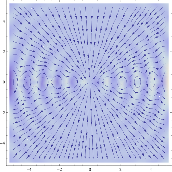
Refer to caption — Figure 4: Spin, orbital and total currents for the ground state of a trapped particle with Weyl coupling, with $j=\frac{1}{2}$ , $m=\frac{1}{2}$ and $v=5$ . In all figures the plane defined by $y=0$ plotted. The arrows represent flows of the local normalized current vector. The color image represents the out of plane component of the spin textures. All three currents are azimuthally symmetric (a) The spin currents have oscillations on the length scale $r\sim 1/v$ . On the axis with $z=0$ , the local spin vector is polarized entirely out of plane at solutions to $\tan rv=-rv/v^{2}$ . The odd solutions feature in-plane vortex loops of spin, while the spin forms anti-vortices at the even solutions. (b) The orbitals are dominated by the in-plane component, which is stronger than the out of plane components by a factor of $v$ . A small out of plane component is largest on the $z=0$ axis. In the upper half plane with $y>0$ , current converges on the point $r=0$ , while on the lower half plane all the current diverges away from the point $r=0$ . (c) The total current is the sum of orbital and spin currents. The total, spin and orbital currents are all independently conserved.

III.1.1 Momentum Space

The azimuthal component of the spinor $\chi_{\frac{1}{2}\frac{1}{2}}^{+}$ suggests the Weyl coupling should have a non-zero current in the ground state. We first define the current operator in momentum space in the standard way. First we multiply Schrödinger’s equation by $\psi^{\dagger}$ , $-i\psi^{\dagger}\frac{\partial}{\partial t}\psi=\psi^{\dagger}\left[-\frac{\nabla_{\mathbf{p}}^{2}}{2}+\frac{\mathbf{p}^{2}}{2}\right]\psi+v\mathbf{p}\cdot\left(\psi^{\dagger}\boldsymbol{\sigma}\psi\right)$ , and subtract the result from it’s complex conjugate. The momentum-space continuity equation is

\displaystyle\partial_{t}\left(\psi^{\dagger}\psi\right)

\displaystyle=

\displaystyle\nabla_{\mathbf{p}}\cdot\mathbf{j}_{\mathbf{p}}

(29)

where

\mathbf{j}_{\mathbf{p}}=\left(-\frac{i}{2}\right)\left[\psi^{\dagger}\nabla_{\mathbf{p}}\psi-\psi^{T}\nabla_{\mathbf{p}}\psi^{*}\right]=\Im\left[\psi^{\dagger}\nabla_{\mathbf{p}}\psi\right]

(30)

is the momentum-space current density. We find that the ground state current in momentum space is given by

\mathbf{j}_{\mathbf{p}}=\pm\frac{\sin\theta}{p}\frac{e^{-(p-v)^{2}}}{4\pi}\hat{\phi}

(31)

for a state with $m=\pm\frac{1}{2}$ .

III.1.2 Position Space

In position space, the spin-orbit coupling is imaginary, so the continuity equation will have contributions from the orbital and spin degrees of freedom:

\displaystyle\mathbf{j}

\displaystyle=

\displaystyle\mathbf{j}_{0}+\mathbf{j}_{s}

(32)

where the orbital current $\mathbf{j}_{0}=\Im\left[\psi^{\dagger}\nabla\psi\right]$ is analogous to the orbital current in momentum space space, and the spin current is $\mathbf{j}_{s}=v\left(\psi^{\dagger}\boldsymbol{\mathbf{\sigma}}\sigma\right)$ . For an eigenstate of the trapped Weyl Hamiltonian, these currents are azimuthally symmetric. The ground state currents can be calculated exactly for large spin-orbit coupling, and are given by

	$\displaystyle\mathbf{j}_{0}$	$\displaystyle=$	$\displaystyle\frac{1}{4\pi}\left[\left(f_{0}^{+}\partial_{r}f_{0}^{-}-f_{0}^{-}\partial_{r}f_{0}^{+}\right)\cos\theta\hat{r}+\sin\theta\frac{f_{0}^{+}}{r}\left(f_{0}^{-}\hat{\theta}+f_{0}^{+}\hat{\phi}\right)\right]$		(33)
	$\displaystyle\mathbf{j}_{s}$	$\displaystyle=$	$\displaystyle\frac{v}{4\pi}\left[\left(\left(f_{0}^{+}\right)^{2}\cos\theta-\left(f_{0}^{-}\right)^{2}\sin\theta\right)\hat{r}+\left(\left(f_{0}^{+}\right)^{2}\sin\theta+\left(f_{0}^{-}\right)^{2}\cos\theta\right)\hat{\theta}+\left(2f_{0}^{+}f_{0}^{-}\sin\theta\right)\hat{\phi}\right]$		(34)

for the ground state with $j=\frac{1}{2}$ and $m=\frac{1}{2}$ . These currents are shown in Fig.4. For a plane defined by fixed $\phi$ , both currents are azimuthally invariant: that is the current fields do not change forms under a rotation by $\phi$ . Since the length scale $1/v$ appears only in the radial variable, the radial component of the orbital current will be stronger than the polar and azimuthal component by a factor of $v$ . As is seen in Fig. 4(b), the out of plane component of spin is negligible only near the plane defined by $\theta=\pi/2$ . The lower half-plane has all currents flowing to the point $r=0$ , while all currents in the upper half plane diverge from this point.

The spin currents do have an out of plane, or azimuthal, component of spin. The in-plane component has a similar structure to the orbital current, in the lower half-plane the current converges to $r=0$ , while it diverges from the point $r=0$ in the upper half plane. The out-of-plane component oscillates on the scale $r\sim 1/v$ with amplitude $\cos\theta$ . At special points corresponding to the solutions of $\tan rv=-rv/v^{2}$ , the out of plane spin current is completely polarized in the azimuthal direction. The sum of the two currents is seen in Fig. 4(c). Since the orbital and spin currents are independently conserved, the total current is also conserved.

IV Conclusion

The problem of the three-dimensional spin-orbit coupling in a harmonic trap was considered. The system has a conserved total angular momentum that allows the Hamiltonian to be projected into sectors where $j,m$ are good quantum numbers. Each sector is tri-diagonal, providing for an efficient numerical calculation of the spectrum. At large values of the spin-orbit coupling parameter, the system undergoes a dimensional reduction from three to one. The spectrum is well approximated by Landau levels in the radial coordinate, with splittings inversely proportional the the spin-orbit coupling strength.

The conservation of total angular momentum allows us to express Schrödinger’s equation as a set of coupled differential equations in the radial coordinate. We find the form of these differential equations in both position and momentum space. Using asymptotic analysis on the momentum space differential equations, we reproduce an analytic spectrum that well approximates the spectrum found numerically. We further use this approximation to find analytical expressions for the low energy eigenfunctions in both position and momentum space.

Finally, we explore the properties of the ground state wavefunction. We find a momentum space orbital current in the azimuthal direction. In position space the total current can be decomposed into a spin current and an orbital current. All currents are invariant under azimuthal rotation. At large spin-orbit coupling, the spin currents have an azimuthal component that oscillates on the inverse of the spin-orbit strength. Along the $z=0$ axis, the spin currents alternate between complete polarization with and against the azimuthal plane. At these special points, the in plane spin density has vortex and anti-vortex structure. The orbital current is characterized by a convergence of all currents at the point $r=0$ in the upper half-sphere, with a divergence of away from the same point in the lower half-sphere.

A single trapped particle with Weyl coupling has rich ground state textures. This suggests that a system of trapped bosonic atoms with Weyl coupling will have novel many-body phases. Early evidence shows such a system will have qualitatively new ground states, such as a cubic lattice phase. [33, 34, 35]

V Acknowledgements

During the completion of this manuscript, the authors became aware of two similar works that reproduce the skyrmion spin textures.[35, 34]

This research was performed in part under the sponsorship of the US Department of Commerce, National Institute of Standards and Technology, and was supported by the National Science Foundation under Physics Frontiers Center Grant PHY-0822671 and by the ARO under the DARPA OLE program.

References

[1] Y. J. Lin, R. L. Compton, K. Jimenez-Garcia, J. V. Porto, and I. B. Spielman, Nature 462, 628 (2009a).
[2] Y.-J. Lin, R. L. Compton, A. R. Perry, W. D. Phillips, J. V. Porto, and I. B. Spielman, Phys. Rev. Lett. 102, 130401 (2009b).
[3] Y. J. Lin, K. Jimenez-Garcia, and I. B. Spielman, Nature 471, 83 (2011a).
[4] Y.-J. Lin, R. L. Compton, K. Jimenez-Garcia, W. D. Phillips, J. V. Porto, and I. B. Spielman, Nat Phys 7, 531 (2011b).
[5] M. Aidelsburger, M. Atala, S. Nascimbène, S. Trotzky, Y.-A. Chen, and I. Bloch, Phys. Rev. Lett. 107, 255301 (2011).
[6] D. L. Campbell, G. Juzeliūnas, and I. B. Spielman, Phys. Rev. A 84, 025602 (2011).
[7] J. Ruseckas, G. Juzeliūnas, P. Öhberg, and M. Fleischhauer, Phys. Rev. Lett. 95, 010404 (2005).
[8] G. Juzeliūnas, J. Ruseckas, and J. Dalibard, Phys. Rev. A 81, 053403 (2010).
[9] J. Dalibard, F. Gerbier, G. Juzeliūnas, and P. Öhberg, Rev. Mod. Phys. 83, 1523 (2011).
[10] T. D. Stanescu, B. Anderson, and V. Galitski, Phys. Rev. A 78, 023616 (2008).
[11] T. D. Stanescu, C. Zhang, and V. Galitski, Phys. Rev. Lett. 99, 110403 (2007).
[12] H. Hu, B. Ramachandhran, H. Pu, and X.-J. Liu, Phys. Rev. Lett. 108, 010402 (2012).
[13] B. Ramachandhran, B. Opanchuk, X.-J. Liu, H. Pu, P. D. Drummond, and H. Hu, Phys. Rev. A 85, 023606 (2012).
[14] S. Sinha, R. Nath, and L. Santos, Physical Review Letters 107, 270401 (2011), arXiv:1109.2045 [cond-mat.quant-gas] .
[15] S. K. Ghosh, J. P. Vyasanakere, and V. B. Shenoy, Phys. Rev. A 84, 053629 (2011).
[16] Y. Li, X. Zhou, and C. Wu, Phys. Rev. B 85, 125122 (2012).
[17] E. Cappelluti, C. Grimaldi, and F. Marsiglio, Phys. Rev. Lett. 98, 167002 (2007).
[18] A. V. Chaplik and L. I. Magarill, Phys. Rev. Lett. 96, 126402 (2006).
[19] J. P. Vyasanakere and V. B. Shenoy, New Journal of Physics 14, 043041 (2012).
[20] X. Cui, ArXiv e-prints (2011), arXiv:1112.1122 [cond-mat.quant-gas] .
[21] S. Takei, C.-H. Lin, B. M. Anderson, and V. Galitski, ArXiv e-prints (2011), arXiv:1111.2340 [cond-mat.quant-gas] .
[22] J. P. Vyasanakere and V. B. Shenoy, Phys. Rev. B 83, 094515 (2011).
[23] M. Gong, S. Tewari, and C. Zhang, Phys. Rev. Lett. 107, 195303 (2011).
[24] Z.-Q. Yu and H. Zhai, Phys. Rev. Lett. 107, 195305 (2011).
[25] J. P. Vyasanakere, S. Zhang, and V. B. Shenoy, Phys. Rev. B 84, 014512 (2011).
[26] R. Barnett, S. Powell, T. Graß, M. Lewenstein, and S. Das Sarma, Phys. Rev. A 85, 023615 (2012).
[27] B. M. Anderson, G. Juzeliūnas, I. B. Spielman, and V. M. Galitski, ArXiv e-prints (2011), arXiv:1112.6022 [cond-mat.quant-gas] .
[28] A. Bermudez, L. Mazza, M. Rizzi, N. Goldman, M. Lewenstein, and M. A. Martin-Delgado, Phys. Rev. Lett. 105, 190404 (2010).
[29] X. Wan, A. M. Turner, A. Vishwanath, and S. Y. Savrasov, Phys. Rev. B 83, 205101 (2011).
[30] E. R. Marshalek, Journal of Mathematical Physics 33, 2972 (1992).
[31] “Digital library of mathematical functions,” National Institute of Standards and Technology, http://dlmf.nist.gov/18.3.T1 (2012a).
[32] “Digital library of mathematical functions,” National Institute of Standards and Technology, http://dlmf.nist.gov/10.47 (2012b).
[33] B. M. Anderson and C. W. Clark, To be published. (2012).
[34] Y. Li, X. Zhou, and C. Wu, ArXiv e-prints (2012), arXiv:1205.2162 [cond-mat.quant-gas] .
[35] T. Kawakami, T. Mizushima, M. Nitta, and K. Machida, ArXiv e-prints (2012), arXiv:1204.3177 [cond-mat.quant-gas] .

VI Appendix A

In this appendix we show that $\mathcal{A}^{+}$ and $\mathcal{A}^{-}$ have the matrix elements as described by Eq.7 and 8. To do this, we first need to calculate the matrix elements of the three-dimensional isotropic harmonic oscillator basis, $\langle n^{\prime}l^{\prime}m^{\prime}|a_{q}|nlm\rangle$ and $\langle n^{\prime}l^{\prime}m^{\prime}|a_{q}^{\dagger}|nlm\rangle$ , where $q=0,\pm 1$ , and the states $|nlm\rangle$ are the states three-dimensional harmonic oscillator basis as defined in the main text.

It is convenient to define the number basis $\left|n,l,m_{l}\right\rangle$ where $(n,l,m_{l})$ are respectively the radial, angular and magnetic quantum numbers. In the absence of spin-orbit coupling we have the harmonic oscillator energies $E=\hbar\omega\left(2n+l+\frac{3}{2}\right)$ where a state of angular momentum $l$ has a $2l+1$ -fold degeneracy of $m_{l}$ . To do this we define the spherical creation and annihilation operators $a_{\pm}=\mp\frac{1}{\sqrt{2}}\left(a_{x}\mp ia_{y}\right)$ , $a_{\pm}^{\dagger}=\mp\frac{1}{\sqrt{2}}\left(a_{x}^{\dagger}\pm ia_{y}^{\dagger}\right)$ , and $a_{0}=a_{z}$ , $a_{0}^{\dagger}=a_{z}^{\dagger}$ . We will find it helpful to express the angular momentum generators as

$\displaystyle L_{+}$	$\displaystyle=$	$\displaystyle\sqrt{2}\left(a_{+}^{\dagger}a_{z}+a_{z}^{\dagger}a_{-}\right),$	(35)
$\displaystyle L_{-}$	$\displaystyle=$	$\displaystyle\sqrt{2}\left(a_{-}^{\dagger}a_{z}+a_{z}^{\dagger}a_{+}\right),$	(36)
$\displaystyle L_{z}$	$\displaystyle=$	$\displaystyle a_{+}^{\dagger}a_{+}-a_{-}^{\dagger}a_{-}$	(37)

with $L_{x}=\frac{1}{2}\left(L_{+}+L_{-}\right)$ and $L_{y}=-\frac{i}{2}\left(L_{+}-L_{-}\right)$ . If we additionally define the operators

$\displaystyle S_{+}$	$\displaystyle=$	$\displaystyle\frac{1}{2}\left(a_{0}^{\dagger}\right)^{2}-a_{+}^{\dagger}a_{-}^{\dagger}$	(38)
$\displaystyle S_{-}$	$\displaystyle=$	$\displaystyle\frac{1}{2}\left(a_{0}\right)^{2}-a_{+}a_{-}$	(39)
$\displaystyle S_{0}$	$\displaystyle=$	$\displaystyle\frac{1}{2}\left(\hat{N}+\frac{3}{2}\right)$	(40)

These operators commute with the angular momentum operators, and satisfy the commutation relations $[S_{+},S_{-}]=-2S_{0}$ and $[S_{0},S_{\pm}]=\pm S_{\pm}$ . The three-dimensional harmonic oscillator eigenstates can be expressed as

|nlm\rangle=\left[\frac{\Gamma\left(l+\frac{3}{2}\right)}{n!\Gamma\left(n+l+\frac{3}{2}\right)}\frac{(l+m)!}{(2l)!(l-m)!}\right]S_{+}^{n}L_{-}^{l-m}|0,l,l\rangle

(41)

where $|0,l,l\rangle=\frac{1}{\sqrt{l!}}\left(a_{+}^{\dagger}\right)^{l}|0,0,0\rangle$ is a state of maximum angular momentum. It can be seen that a state $|nlm\rangle$ has energy $E=2n+l+\frac{3}{2}$ .

VI.1 Caculation of: $a_{q}^{\dagger}$

To calculate $a_{-}^{\dagger}$ , we first note that the operator changes the total energy number by $\Delta n=+1$ unit, so it must connect states with either $\Delta n=+1$ and $\Delta l=-1$ , or $\Delta n=0$ and $\Delta l=+1$ . Other states with $\Delta n>1$ and $\Delta l=-1+2(\Delta n-1)$ are consistent with this condition, but must have zero matrix elements from the fact that $a_{q}$ is a spherical tensor of rank-1, and higher order corrections are inconsistent with angular momentum conservation. Using this fact, the matrix elements can be decomposed as

	$\displaystyle\left\langle n^{\prime},l^{\prime},m^{\prime}\right\|a_{-}^{\dagger}\left\|n,l,m\right\rangle$	$\displaystyle=$	$\displaystyle\left\langle n,l+1,m-1\right\|a_{-}^{\dagger}\left\|n,l,m\right\rangle\delta_{n^{\prime},n}\delta_{l^{\prime},l+1}\delta_{m^{\prime},m-1}$		(42)
		$\displaystyle+$	$\displaystyle\left\langle n+1,l-1,m-1\right\|a_{-}^{\dagger}\left\|n,l,m\right\rangle\delta_{n^{\prime},n+1}\delta_{l^{\prime},l-1}\delta_{m^{\prime},m-1}$		(43)

The two non-zero elements can be calculated individually. We first calculate $\left\langle n,l+1,m-1\right|a_{-}^{\dagger}\left|n,l,m\right\rangle$ . It is convenient to use the equivalent definition of $\left|n,l,m\right\rangle$ , given by

|nlm\rangle=\left[\frac{\Gamma\left(l+\frac{3}{2}\right)}{n!\Gamma\left(n+l+\frac{3}{2}\right)}\frac{(l-m)!}{(2l)!(l+m)!}\right]S_{+}^{n}L_{-}^{l+m}|0,l,-l\rangle

(44)

to express the desired element as

	$\displaystyle\left\langle n,l+1,m-1\right\|a_{-}^{\dagger}\left\|n,l,m\right\rangle$	$\displaystyle=$	$\displaystyle\tilde{\mathcal{N}}_{n,l+1,m-1}\tilde{\mathcal{N}}_{n,l,m}\left\langle{\bf 0}\right\|(a_{-})^{l+1}(L_{-})^{l+m}(S_{-})^{n}a_{-}^{\dagger}(S_{+})^{n}(L_{+})^{l+m}(a_{-}^{\dagger})^{l}\left\|{\bf 0}\right\rangle$		(45)
		$\displaystyle=$	$\displaystyle\tilde{\mathcal{N}}_{n,l+1,m-1}\tilde{\mathcal{N}}_{n,l,m}\left\langle{\bf 0}\right\|(a_{-})^{l+1}(L_{-})^{l+m}(S_{-})^{n}(S_{+})^{n}a_{-}^{\dagger}(L_{+})^{l+m}(a_{-}^{\dagger})^{l}\left\|{\bf 0}\right\rangle$		(46)

where the normalization constant is $\tilde{\mathcal{N}}_{n,l,m}=\left[\frac{\Gamma\left(l+\frac{3}{2}\right)}{n!\Gamma\left(n+l+\frac{3}{2}\right)}\frac{(l-m)!}{(2l)!(l+m)!}\right]$ , and we have used the commutation relation $[a_{-}^{\dagger},S_{+}]=0$ . The bra $\left\langle 0\right|(a_{-})^{l+1}(L_{-})^{l+m}$ is an eigenbra of the the operator $\left(S_{-}\right)^{n}\left(S_{+}\right)^{n}$ with eigenvalue $\frac{n!\Gamma(n+l+3/2+1)}{\Gamma(l+3/2+1)}$ . We can again use the commutation of the operator $[L_{-},a_{-}^{\dagger}]=0$ to find the remaining factor

$\displaystyle\left\langle{\bf 0}\right\|(a_{-})^{l+1}(L_{-})^{l+m}a_{-}^{\dagger}(L_{+})^{l+m}(a_{-}^{\dagger})^{l}\left\|{\bf 0}\right\rangle$	$\displaystyle=$	$\displaystyle\left\langle{\bf 0}\right\|(a_{-})^{l+1}a_{-}^{\dagger}(L_{-})^{l+m}(L_{+})^{l+m}(a_{-}^{\dagger})^{l}\left\|{\bf 0}\right\rangle$	(47)
	$\displaystyle=$	$\displaystyle(l+1)\left\langle{\bf 0}\right\|(a_{-})^{l}(L_{-})^{l+m}(L_{+})^{l+m}(a_{-}^{\dagger})^{l}\left\|{\bf 0}\right\rangle$	(48)
	$\displaystyle=$	$\displaystyle(l+1)\tilde{\mathcal{N}}_{0,l,m}^{-2}.$	(49)

These factors combine to give the non-zero value of the matrix element

\left\langle n,l+1,m-1\right|a_{-}^{\dagger}\left|n,l,m\right\rangle=\frac{1}{2}\sqrt{\frac{n+l+3/2}{l+3/2}\frac{(l-m+2)(l-m+1)}{l+1/2}}.

(50)

Similar techniques can applied to evaluate the other non-zero matrix element of the operator $a_{-}^{\dagger}$ . The calculation is straightforward using the same techniques. The full matrix element is given by

	$\displaystyle\left\langle n^{\prime},l^{\prime},m^{\prime}\right\|a_{-}^{\dagger}\left\|n,l,m\right\rangle$	$\displaystyle=$	$\displaystyle\frac{1}{2}\sqrt{\frac{n+l+3/2}{l+3/2}\frac{(l-m+2)(l-m+1)}{l+1/2}}\delta_{n^{\prime},n}\delta_{l^{\prime},l+1}\delta_{m^{\prime},m-1}$		(51)
		$\displaystyle-$	$\displaystyle\frac{1}{2}\sqrt{\frac{n+1}{l+1/2}\frac{(l+m)(l+m-1)}{l-1/2}}\delta_{n^{\prime},n+1}\delta_{l^{\prime},l-1}\delta_{m^{\prime},m-1}.$		(52)

The remaining matrix elements can be calculated in an analogous way. The results can be summarized by the expression

\displaystyle a_{q}^{\dagger}\left|n,l,m\right\rangle

\displaystyle=

\displaystyle c_{q}^{+}(n,l,m)\left|n,l+1,m+q\right\rangle+d_{q}^{+}(n,l,m)\left|n+1,l-1,m+q\right\rangle

(53)

where $q=-1,0,1$ , and the matrix elements are given by

$\displaystyle c_{q}^{-}(n,l,m)$	$\displaystyle=$	$\displaystyle\left(\frac{1}{\sqrt{2}}\right)^{1+\|q\|}\sqrt{\frac{n+l+1/2}{(l+1/2)(l-1/2)}}f_{q}(l,m)$	(54)
$\displaystyle d_{q}^{-}(n,l,m)$	$\displaystyle=$	$\displaystyle(-1)^{q}\left(\frac{1}{\sqrt{2}}\right)^{1+\|q\|}\sqrt{\frac{n}{(l+3/2)(l+1/2)}}g_{-q}(l,m)$	(55)
$\displaystyle c_{q}^{+}(n,l,m)$	$\displaystyle=$	$\displaystyle\left(\frac{1}{\sqrt{2}}\right)^{1+\|q\|}\sqrt{\frac{n+l+3/2}{(l+3/2)(l+1/2)}}g_{q}(l,m)$	(56)
$\displaystyle d_{q}^{+}(n,l,m)$	$\displaystyle=$	$\displaystyle(-1)^{q}\left(\frac{1}{\sqrt{2}}\right)^{1+\|q\|}\sqrt{\frac{n+1}{(l+1/2)(l-1/2)}}f_{-q}(l,m)$	(57)

where the functions $f_{q}(l,m)$ and $g_{q}(l,m)$ are defined as

	$\displaystyle f_{q}(l,m)$	$\displaystyle=$	$\displaystyle\left\{\begin{array}[]{ll}\sqrt{(l+m)(l+m-1)}&q=+1\\ \sqrt{(l+m)(l-m)}&q=0\\ \sqrt{(l-m)(l-m-1)}&q=-1\end{array}\right.$
	$\displaystyle g_{q}(l,m)$	$\displaystyle=$	$\displaystyle\left\{\begin{array}[]{ll}\sqrt{(l+m+2)(l+m+1)}&q=+1\\ \sqrt{(l+m+1)(l-m+1)}&q=0\\ \sqrt{(l-m+2)(l-m+1)}&q=-1\end{array}\right..$

The matrix elements of the operators $a_{q}$ can be calculated through conjugation.

VI.2 Matrix elements of $\mathcal{A}^{+}$ and $\mathcal{A}^{-}$ .

We can now calculate the matrix elements of $\mathcal{A}^{+}$ and $\mathcal{A}^{-}$ for states of good total angular momentum labeled by quantum numbers $j,m$ . Recall in the main text that these states are defined by

\left|n,j,m,\lambda\right\rangle=e^{i\phi_{\lambda}}\begin{pmatrix}\lambda\sqrt{\frac{j-\lambda m+x_{\lambda}}{2(j+x_{\lambda})}}\left|n,j+\frac{\lambda}{2},m-\frac{1}{2}\right\rangle\\ -\sqrt{\frac{j+\lambda m+x_{\lambda}}{2(j+x_{\lambda})}}\left|n,j+\frac{\lambda}{2},m+\frac{1}{2}\right\rangle\end{pmatrix}

(66)

where $\phi_{\lambda}$ is an arbitrary phase. We will find it convenient to express this as

\left|n,j,m,\lambda\right\rangle=\begin{pmatrix}\gamma_{\lambda}^{\uparrow}\left|n,j+\frac{\lambda}{2},m-\frac{1}{2}\right\rangle\\ \gamma_{\lambda}^{\downarrow}\left|n,j+\frac{\lambda}{2},m+\frac{1}{2}\right\rangle\end{pmatrix},

(67)

where $\gamma_{\lambda}^{\uparrow}=\lambda e^{i\phi_{\lambda}}\sqrt{\frac{j-\lambda m+x_{\lambda}}{2(j+x_{\lambda})}}$ and $\gamma_{\lambda}^{\downarrow}=-e^{i\phi_{\lambda}}\sqrt{\frac{j+\lambda m+x_{\lambda}}{2(j+x_{\lambda})}}$ .

We now consider the action of the operator $\boldsymbol{\sigma}\cdot\mathbf{p}$ on the states $\left|n,j,m,\lambda\right\rangle$ ,

$\displaystyle\left(\sqrt{2}\left(\sigma_{-}a_{-}-\sigma_{+}a_{+}\right)+\sigma_{z}a_{z}\right)\left\|n,j,m,\lambda\right\rangle$	$\displaystyle=$	$\displaystyle\begin{pmatrix}-\sqrt{2}\gamma_{\lambda}^{\downarrow}a_{+}\left\|n,j+\frac{\lambda}{2},m+\frac{1}{2}\right\rangle+\gamma_{\lambda}^{\uparrow}a_{z}\left\|n,j+\frac{\lambda}{2},m-\frac{1}{2}\right\rangle\\ \sqrt{2}\gamma_{\lambda}^{\uparrow}a_{-}\left\|n,j+\frac{\lambda}{2},m-\frac{1}{2}\right\rangle-\gamma_{\lambda}^{\downarrow}a_{z}\left\|n,j+\frac{\lambda}{2},m+\frac{1}{2}\right\rangle\end{pmatrix}$	(68)
	$\displaystyle=$	$\displaystyle\begin{pmatrix}\left(-\sqrt{2}\gamma_{\lambda}^{\downarrow}c_{+}^{-}(n,j+\frac{\lambda}{2},m+\frac{1}{2})+\gamma_{\lambda}^{\uparrow}c_{0}^{-}(n,j+\frac{\lambda}{2},m-\frac{1}{2})\right)\left\|n,j-1+\frac{\lambda}{2},m-\frac{1}{2}\right\rangle\\ \left(\sqrt{2}\gamma_{\lambda}^{\uparrow}c_{-}^{-}(n,j+\frac{\lambda}{2},m-\frac{1}{2})-\gamma_{\lambda}^{\downarrow}c_{0}^{-}(n,j+\frac{\lambda}{2},m+\frac{1}{2})\right)\left\|n,j-1+\frac{\lambda}{2},m+\frac{1}{2}\right\rangle\end{pmatrix}$	(69)
	$\displaystyle+$	$\displaystyle\begin{pmatrix}\left(-\sqrt{2}\gamma_{\lambda}^{\downarrow}d_{+}^{-}(n,j+\frac{\lambda}{2},m+\frac{1}{2})+\gamma_{\lambda}^{\uparrow}d_{0}^{-}(n,j+\frac{\lambda}{2},m-\frac{1}{2})\right)\left\|n-1,j+1+\frac{\lambda}{2},m-\frac{1}{2}\right\rangle\\ \left(\sqrt{2}\gamma_{\lambda}^{\uparrow}d_{-}^{-}(n,j+\frac{\lambda}{2},m-\frac{1}{2})-\gamma_{\lambda}^{\downarrow}d_{0}^{-}(n,j+\frac{\lambda}{2},m+\frac{1}{2})\right)\left\|n-1,j+1+\frac{\lambda}{2},m+\frac{1}{2}\right\rangle\end{pmatrix}.$	(70)

This can be expressed as

\displaystyle\left(\sqrt{2}\left(\sigma_{-}a_{-}-\sigma_{+}a_{+}\right)+\sigma_{z}a_{z}\right)\left|n,j,m,\lambda\right\rangle

\displaystyle=

\displaystyle\begin{pmatrix}\Gamma_{c}^{\uparrow}(\lambda)\left|n,j-1+\frac{\lambda}{2},m-\frac{1}{2}\right\rangle\\ \Gamma_{c}^{\downarrow}(\lambda)\left|n,j-1+\frac{\lambda}{2},m+\frac{1}{2}\right\rangle\end{pmatrix}+\begin{pmatrix}\Gamma_{d}^{\uparrow}(\lambda)\left|n-1,j+1+\frac{\lambda}{2},m-\frac{1}{2}\right\rangle\\ \Gamma_{d}^{\downarrow}(\lambda)\left|n-1,j+1+\frac{\lambda}{2},m+\frac{1}{2}\right\rangle\end{pmatrix},

(71)

where the coefficients

$\displaystyle\Gamma_{c}^{\uparrow}(\lambda)$	$\displaystyle=$	$\displaystyle\left(-\sqrt{2}\gamma_{\lambda}^{\downarrow}c_{+}^{-}\left(n,j+\frac{\lambda}{2},m+\frac{1}{2}\right)+\gamma_{\lambda}^{\uparrow}c_{0}^{-}\left(n,j+\frac{\lambda}{2},m-\frac{1}{2}\right)\right)$	(72)
	$\displaystyle=$	$\displaystyle-e^{i\phi_{\lambda}}\sqrt{\frac{n+j+\frac{\lambda}{2}+\frac{1}{2}}{2(j+\frac{\lambda}{2}+\frac{1}{2})(j+\frac{\lambda}{2}-\frac{1}{2})}}\left(-f_{+}\left(j+\frac{\lambda}{2},m+\frac{1}{2}\right)\gamma_{\lambda}^{\downarrow}+f_{0}\left(j+\frac{\lambda}{2},m-\frac{1}{2}\right)\gamma_{\lambda}^{\uparrow}\right)$	(73)
	$\displaystyle=$	$\displaystyle e^{i\phi_{\lambda}}\sqrt{\frac{\left(n+j+x_{\lambda}\right)\left(j+m+x_{\lambda}-1\right)}{4(j+x_{\lambda})^{2}(j+x_{\lambda}-1)}}\left(\sqrt{\left(j+\lambda m+x_{\lambda}\right)\left(j+m+x_{\lambda}\right)}+\lambda\sqrt{\left(j-\lambda m+x_{\lambda}\right)\left(j-m+x_{\lambda}\right)}\right)$	(74)

and

$\displaystyle\Gamma_{c}^{\downarrow}(\lambda)$	$\displaystyle=$	$\displaystyle\left(\sqrt{2}\gamma_{\lambda}^{\uparrow}c_{-}^{-}\left(n,j+\frac{\lambda}{2},m-\frac{1}{2}\right)-\gamma_{\lambda}^{\downarrow}c_{0}^{-}\left(n,j+\frac{\lambda}{2},m+\frac{1}{2}\right)\right)$	(75)
	$\displaystyle=$	$\displaystyle-e^{i\phi_{\lambda}}\sqrt{\frac{n+j+\frac{\lambda}{2}+\frac{1}{2}}{2(j+\frac{\lambda}{2}+\frac{1}{2})(j+\frac{\lambda}{2}-\frac{1}{2})}}\left(-f_{-}\left(j+\frac{\lambda}{2},m-\frac{1}{2}\right)\gamma_{\lambda}^{\uparrow}-f_{0}\left(j+\frac{\lambda}{2},m+\frac{1}{2}\right)\gamma_{\lambda}^{\downarrow}\right)$	(76)
	$\displaystyle=$	$\displaystyle e^{i\phi_{\lambda}}\sqrt{\frac{\left(n+j+x_{\lambda}\right)\left(j-m+x_{\lambda}-1\right)}{4(j+x_{\lambda})^{2}(j+x_{\lambda}-1)}}\left(\lambda\sqrt{\left(j-\lambda m+x_{\lambda}\right)\left(j-m+x_{\lambda}\right)}+\sqrt{\left(j+\lambda m+x_{\lambda}\right)\left(j+m+x_{\lambda}\right)}\right).$	(77)

Explicitly calculating these for $\lambda=\pm 1$ we get:

	$\displaystyle\left(\sqrt{2}\gamma_{+}^{\downarrow}c_{+}^{-}\left(n,j+\frac{1}{2},m+\frac{1}{2}\right)+\gamma_{+}^{\uparrow}c_{0}^{-}\left(n,j+\frac{1}{2},m-\frac{1}{2}\right)\right)$	$\displaystyle=$	$\displaystyle e^{i\phi_{+}}\sqrt{2(n+j+1)}\sqrt{\frac{j+m}{2j}}$		(78)
	$\displaystyle\left(\sqrt{2}\gamma_{-}^{\downarrow}c_{+}^{-}\left(n,j-\frac{1}{2},m+\frac{1}{2}\right)+\gamma_{-}^{\uparrow}c_{0}^{-}\left(n,j-\frac{1}{2},m-\frac{1}{2}\right)\right)$	$\displaystyle=$	$\displaystyle 0$		(79)

and

	$\displaystyle\left(\sqrt{2}\gamma_{+}^{\uparrow}c_{-}^{-}\left(n,j+\frac{1}{2},m-\frac{1}{2}\right)-\gamma_{+}^{\downarrow}c_{0}^{-}\left(n,j+\frac{1}{2},m+\frac{1}{2}\right)\right)$	$\displaystyle=$	$\displaystyle e^{i\phi_{+}}\sqrt{2(n+j+1)}\sqrt{\frac{j-m}{2j}}$		(80)
	$\displaystyle\left(\sqrt{2}\gamma_{-}^{\uparrow}c_{-}^{-}\left(n,j-\frac{1}{2},m-\frac{1}{2}\right)-\gamma_{-}^{\downarrow}c_{0}^{-}\left(n,j-\frac{1}{2},m+\frac{1}{2}\right)\right)$	$\displaystyle=$	$\displaystyle 0.$		(81)

Similarly, we calculate the equivalent terms for $\Gamma_{d}^{s}(\lambda)$ with $s=\uparrow,\downarrow$ . This gives

	$\displaystyle\Gamma_{d}^{\uparrow}(\lambda)$	$\displaystyle=$	$\displaystyle\left(-\sqrt{2}\gamma_{\lambda}^{\downarrow}d_{+}^{-}\left(n,j+\frac{\lambda}{2},m+\frac{1}{2}\right)+\gamma_{\lambda}^{\uparrow}d_{0}^{-}\left(n,j+\frac{\lambda}{2},m-\frac{1}{2}\right)\right)$		(82)
		$\displaystyle=$	$\displaystyle e^{i\phi_{\lambda}}\sqrt{\frac{n\left(j-m+x_{\lambda}+1\right)}{4(j+x_{\lambda})^{2}(j+x_{\lambda}+1)}}\left(\sqrt{\left(j+\lambda m+x_{\lambda}\right)\left(j-m+x_{\lambda}\right)}-\lambda\sqrt{\left(j-\lambda m+x_{\lambda}\right)\left(j+m+x_{\lambda}\right)}\right)$		(83)

	$\displaystyle\Gamma_{d}^{\downarrow}(\lambda)$	$\displaystyle=$	$\displaystyle\left(\sqrt{2}\gamma_{\lambda}^{\uparrow}d_{-}^{-}\left(n,j+\frac{\lambda}{2},m-\frac{1}{2}\right)-\gamma_{\lambda}^{\downarrow}d_{+}^{0}\left(n,j+\frac{\lambda}{2},m+\frac{1}{2}\right)\right)$		(84)
		$\displaystyle=$	$\displaystyle-e^{i\phi_{\lambda}}\sqrt{\frac{n\left(j+m+x_{\lambda}+1\right)}{4(j+x_{\lambda})^{2}(j+x_{\lambda}+1)}}\left(\lambda\sqrt{\left(j-\lambda m+x_{\lambda}\right)\left(j+m+x_{\lambda}\right)}-\sqrt{\left(j-m+x_{\lambda}\right)\left(j+\lambda m+x_{\lambda}\right)}\right)$		(85)

Explicitly,

	$\displaystyle\Gamma_{d}^{\uparrow}(+)=\left(-\sqrt{2}\gamma_{+}^{\downarrow}d_{+}^{-}\left(n,j+\frac{1}{2},m+\frac{1}{2}\right)+\gamma_{+}^{\uparrow}d_{0}^{-}\left(n,j+\frac{1}{2},m-\frac{1}{2}\right)\right)$	$\displaystyle=$	$\displaystyle 0$		(86)
	$\displaystyle\Gamma_{d}^{\uparrow}(-)=\left(-\sqrt{2}\gamma_{-}^{\downarrow}d_{+}^{-}\left(n,j-\frac{1}{2},m+\frac{1}{2}\right)+\gamma_{-}^{\uparrow}d_{0}^{-}\left(n,j-\frac{1}{2},m-\frac{1}{2}\right)\right)$	$\displaystyle=$	$\displaystyle e^{i\phi_{-}}\sqrt{2n}\sqrt{\frac{j-m+1}{2(j+1)}}$		(87)

	$\displaystyle\Gamma_{d}^{\downarrow}(+)=\left(\sqrt{2}\gamma_{+}^{\uparrow}d_{-}^{-}\left(n,j+\frac{1}{2},m-\frac{1}{2}\right)-\gamma_{+}^{\downarrow}d_{+}^{0}\left(n,j+\frac{1}{2},m+\frac{1}{2}\right)\right)$	$\displaystyle=$	$\displaystyle 0$		(88)
	$\displaystyle\Gamma_{d}^{\downarrow}(-)=\left(\sqrt{2}\gamma_{-}^{\uparrow}d_{-}^{-}\left(n,j-\frac{1}{2},m-\frac{1}{2}\right)-\gamma_{-}^{\downarrow}d_{+}^{0}\left(n,j-\frac{1}{2},m+\frac{1}{2}\right)\right)$	$\displaystyle=$	$\displaystyle e^{i\phi_{-}}\sqrt{2n}\sqrt{\frac{j+m+1}{2(j+1)}}$		(89)

We summarize these relations as (restoring the subscript on $n_{r}$ )

	$\displaystyle\mathcal{A}^{-}\left\|n_{r},j,m,+\right\rangle$	$\displaystyle=$	$\displaystyle e^{i\Delta\phi}\sqrt{2n_{r}}\left\|n_{r}-1,j,m,-\right\rangle$		(90)
	$\displaystyle\mathcal{A}^{-}\left\|n_{r},j,m,-\right\rangle$	$\displaystyle=$	$\displaystyle e^{-i\Delta\phi}\sqrt{2(n_{r}+j+1)}\left\|n_{r},j,m,+\right\rangle$		(91)

where $\Delta\phi=\left(\phi_{+}-\phi_{-}\right)$ . We can find the action of the operator $\mathcal{A}^{+}={\mathcal{A}^{-}}^{\dagger}$ through conjugation

	$\displaystyle\mathcal{A}^{+}\left\|n_{r},j,m,+\right\rangle$	$\displaystyle=$	$\displaystyle e^{-i\Delta\phi}\sqrt{2(n_{r}+j+1)}\left\|n_{r},j,m,-\right\rangle$		(92)
	$\displaystyle\mathcal{A}^{+}\left\|n_{r},j,m,-\right\rangle$	$\displaystyle=$	$\displaystyle e^{i\Delta\phi}\sqrt{2(n_{r}+1)}\left\|n_{r}+1,j,m,+\right\rangle$		(93)

We can show that $\frac{1}{2}\{\mathcal{A}^{+},\mathcal{A}^{-}\}=\hat{N}+3/2$ , so

H=\frac{1}{2}\{\mathcal{A}^{+},\mathcal{A}^{-}\}+i\frac{v}{\sqrt{2}}(\mathcal{A}^{+}-\mathcal{A}^{-}).

(94)

If we chose $e^{i\Delta\phi}=-1$ , we see that the matrix elements for ${\bf p}\cdot\boldsymbol{\sigma}=\frac{i}{\sqrt{2}}\left(\mathcal{A}^{+}-\mathcal{A}^{-}\right)$ are:

	$\displaystyle\langle n_{r}^{\prime},j,m,+\|\frac{i}{\sqrt{2}}\left(\mathcal{A}^{+}-\mathcal{A}^{-}\right)\|n_{r},j,m,-\rangle$	$\displaystyle=$	$\displaystyle i\left(\sqrt{n_{r}+1}\delta_{n_{r}+1,n_{r}^{\prime}}-\sqrt{n_{r}+j+1}\delta_{n_{r},n_{r}^{\prime}}\right)$		(95)
	$\displaystyle\langle n_{r}^{\prime},j,m,-\|\frac{i}{\sqrt{2}}\left(\mathcal{A}^{+}-\mathcal{A}^{-}\right)\|n_{r},j,m,+\rangle$	$\displaystyle=$	$\displaystyle i\left(\sqrt{n_{r}+j+1}\delta_{n_{r},n_{r}^{\prime}}-\sqrt{n_{r}}\delta_{n_{r}-1,n_{r}^{\prime}}\right).$		(96)

VII Appendix B

In this appendix we calculate the radial Schrödinger equation in position space by Fourier transforming the momentum-space version. We want to find the Fourier transform of the eigenfunctions of the harmonic oscillator. We first need to find the momentum space eigenfunctions of the three-dimensional spherical harmonic oscillator int terms of the momentum space harmonic oscillator wavefunctions $\langle\mathbf{p}|\psi_{nlm}\rangle=\int\frac{d\mathbf{r}}{\sqrt{(2\pi)^{3}}}e^{i\mathbf{p}\cdot\mathbf{r}}\langle\mathbf{r}|\psi_{nlm}\rangle$ . Using the expansion of plane waves into spherical harmonics, $e^{i\mathbf{p}\cdot\mathbf{r}}=4\pi\sum_{lm}i^{l}j_{l}(pr)Y_{l}^{m}(\hat{\mathbf{p}})\left(Y_{l}^{m}(\hat{\mathbf{r}})\right)^{*}$ , we find the relation

	$\displaystyle\langle\mathbf{p}\|\psi_{nlm}\rangle$	$\displaystyle=$	$\displaystyle\int\frac{d\mathbf{r}}{\sqrt{(2\pi)^{3}}}4\pi\sum_{l^{\prime}m^{\prime}}i^{l^{\prime}}j_{l^{\prime}}(pr)Y_{l^{\prime}}^{m^{\prime}}(\hat{\mathbf{p}})\left(Y_{l^{\prime}}^{m^{\prime}}(\hat{\mathbf{r}})\right)^{*}\langle\mathbf{r}\|\psi_{nlm}\rangle$		(97)
		$\displaystyle=$	$\displaystyle\sqrt{\frac{2}{\pi}}i^{l}Y_{l}^{m}(\hat{\mathbf{p}})\int dr\left(r^{2}j_{l}(pr)R_{ln}(r)\right).$		(98)

To find the radial Schrödinger’s equation for the Weyl coupling in position space,

\left[-\frac{\nabla_{\mathbf{p}}^{2}}{2}+\frac{\mathbf{p}^{2}}{2}+v\mathbf{p}\cdot\boldsymbol{\sigma}\right]\psi_{njm}(\mathbf{p})=E_{nj}\psi_{njm}(\mathbf{p})

(99)

it is easiest to begin with the same equation in momentum space, and Fourier transform the eigenstates $\psi_{njm}(\mathbf{p})=\int e^{i\mathbf{p}\cdot\mathbf{r}}\phi_{njm}(\mathbf{r)}d\mathbf{r}$ . But recall, we have showed that $j$ and $m$ are good quantum numbers, and the eigenfunctions have the form $\psi_{njm}(\mathbf{p})=f_{n}^{+}(p)\chi_{jm}^{+}(\mathbf{\hat{p}})+f_{n}^{-}(p)\chi_{jm}^{-}(\mathbf{\hat{p}})$ . The spinors $\chi_{jm}^{\pm}$ contain spherical harmonics of order $l=j\mp\frac{1}{2}$ , so they are eigenfunctions of the Fourier transform. The position space wavefunction thus has the form

	$\displaystyle\phi_{njm}(\mathbf{r})$	$\displaystyle=$	$\displaystyle 4\pi\int\frac{d^{3}\mathbf{r}}{\sqrt{(2\pi)^{3}}}\left[\sum_{lm}(-i)^{l}j_{l}(pr)Y_{l}^{m}(\hat{\mathbf{p}})\left(Y_{l}^{m}(\hat{\mathbf{r}})\right)^{*}\right]\left(f_{n}^{+}(p)\chi_{jm}^{+}(\mathbf{\hat{p}})+f_{n}^{-}(p)\chi_{jm}^{-}(\mathbf{\hat{p}})\right)$		(100)
		$\displaystyle=$	$\displaystyle\sqrt{\frac{2}{\pi}}(-i)^{j-\frac{1}{2}}\left(-ig_{n}^{+}(r)\chi_{jm}^{+}(\mathbf{\hat{r}})+g_{n}^{-}(r)\chi_{jm}^{-}(\mathbf{\hat{r}})\right),$		(101)

where $g_{n}^{\pm}(r)=\int p^{2}j_{l}\left(pr\right)f_{n}^{\pm}(p)dp$ , and $l=j\mp\frac{1}{2}$ .

We are now ready to transform the momentum-space Schrödinger equation, we first multiply by $e^{i\mathbf{p}\cdot\mathbf{r}}$ , and then integrate over momentum to get

\displaystyle\int\frac{d^{3}\mathbf{p}}{\sqrt{(2\pi)^{3}}}e^{i\mathbf{p}\cdot\mathbf{r}}\left[-\frac{\nabla_{\mathbf{p}}^{2}}{2}+\frac{\mathbf{p}^{2}}{2}+v\mathbf{p}\cdot\boldsymbol{\sigma}\right]\psi_{njm}(\mathbf{p})

\displaystyle=

\displaystyle E_{nj}\int\frac{d^{3}\mathbf{p}}{\sqrt{(2\pi)^{3}}}e^{i\mathbf{p}\cdot\mathbf{r}}\psi_{njm}(\mathbf{p}).

(102)

Transforming this term-by-term, the momentum space kinetic term becomes a position space trapping term

\displaystyle\int\frac{d^{3}\mathbf{p}}{\sqrt{(2\pi)^{3}}}e^{i\mathbf{p}\cdot\mathbf{r}}\left(\frac{-\nabla_{\mathbf{p}}^{2}}{2}\right)\psi_{njm}(\mathbf{p})

\displaystyle=

\displaystyle\frac{1}{2}\mathbf{r}^{2}\phi_{njm}(\mathbf{r}),

(103)

Similarly, the momentum space trap becomes a kinetic energy term in position space

	$\displaystyle\int\frac{d^{3}\mathbf{p}}{\sqrt{(2\pi)^{3}}}\left(\frac{\mathbf{p}^{2}}{2}\right)e^{i\mathbf{p}\cdot\mathbf{r}}\psi_{njm}(\mathbf{p})$	$\displaystyle=$	$\displaystyle-\frac{\nabla^{2}}{2}\int\frac{d^{3}\mathbf{p}}{\sqrt{(2\pi)^{3}}}\left(\psi_{njm}(\mathbf{p})e^{i\mathbf{p}\cdot\mathbf{r}}\right)$		(104)
		$\displaystyle=$	$\displaystyle-\frac{\nabla^{2}}{2}\phi_{njm}(\mathbf{r}).$		(105)

The spin-orbit term is more complicated, we first use the property that $\mathbf{p}\cdot\boldsymbol{\sigma}\chi_{jm}^{\pm}(\hat{\mathbf{p}})=p\chi_{jm}^{\mp}(\hat{\mathbf{p}})$

\displaystyle\int\frac{d^{3}\mathbf{p}}{\sqrt{(2\pi)^{3}}}\left[e^{i\mathbf{p}\cdot\mathbf{r}}v\left(\mathbf{p}\cdot\boldsymbol{\sigma}\right)\psi_{njm}(\mathbf{p})\right]

\displaystyle=

\displaystyle v\int\frac{d^{3}\mathbf{p}}{\sqrt{(2\pi)^{3}}}\left[e^{i\mathbf{p}\cdot\mathbf{r}}p\left(f_{n}^{+}(p)\chi_{jm}^{-}(\mathbf{\hat{p}})+f_{n}^{-}(p)\chi_{jm}^{+}(\mathbf{\hat{p}})\right)\right],

(106)

we then expand the exponential $e^{i\mathbf{p}\cdot\mathbf{r}}$ in terms of spherical harmonics,

	$\displaystyle\int\frac{d^{3}\mathbf{p}}{\sqrt{(2\pi)^{3}}}\left[e^{i\mathbf{p}\cdot\mathbf{r}}v\left(\mathbf{p}\cdot\boldsymbol{\sigma}\right)\psi_{njm}(\mathbf{p})\right]$	$\displaystyle=$	$\displaystyle v\frac{4\pi}{\sqrt{(2\pi)^{3}}}\sum_{lm}i^{l}\int d\hat{\mathbf{p}}\int dp\,p^{3}\left[j_{l}\left(pr\right)Y_{l}^{m}\left(\hat{\mathbf{r}}\right)\left(Y_{l}^{m}\left(\hat{\mathbf{p}}\right)\right)^{*}\left(f_{n}^{+}(p)\chi_{jm}^{-}(\mathbf{\hat{p}})+f_{n}^{-}(p)\chi_{jm}^{+}(\mathbf{\hat{p}})\right)\right]$		(107)
		$\displaystyle=$	$\displaystyle v\frac{4\pi}{\sqrt{(2\pi)^{3}}}i^{j-\frac{1}{2}}\left[i\int dp\left(p^{3}j_{j+\frac{1}{2}}(pr)f_{nj}^{-}(p)\right)\chi_{jm}^{+}(\hat{\mathbf{r}})+\int dp\left(p^{3}j_{j-\frac{1}{2}}(pr)f_{nj}^{+}(p)\right)\chi_{jm}^{-}(\hat{\mathbf{r}})\right].$		(108)

The spinors $\chi_{jm}^{\pm}$ have angular momentum components $l=j\mp\frac{1}{2}$ . These angular momentum variables do not match the angular momentum corresponding to the spinors multiplying them. This, along with the extra factor of $p$ in the integrand $\int dp\left(p^{3}j_{l}(pr)f(p)\right)=\int dp\,p^{2}\left(pj_{l}(pr)f(p)\right)$ , suggest it would be helpful to express the term $pj_{j_{\pm\frac{1}{2}}}(pr)$ in terms of spherical Bessel functions of the order $j\mp\frac{1}{2}$ . We use the identities

	$\displaystyle zj_{l}(z)$	$\displaystyle=$	$\displaystyle z\frac{d}{dz}j_{l+1}(z)+(l+2)j_{l+1}(z)$		(109)
	$\displaystyle zj_{l}(z)$	$\displaystyle=$	$\displaystyle-z\frac{d}{dz}j_{l-1}(z)+(l-1)j_{l-1}(z)$		(110)

to express

	$\displaystyle pj_{l}(pr)$	$\displaystyle=$	$\displaystyle\left(\frac{d}{dr}+\frac{l+2}{r}\right)j_{l+1}(pr)$		(111)
		$\displaystyle=$	$\displaystyle\left(-\frac{d}{dr}+\frac{l-1}{r}\right)j_{l-1}(pr).$		(112)

These relations convert the product $pj_{l}(pr)$ into a differential operator in $r$ that can be removed from the integral. Together, these give the expression for the Fourier transform of the three-dimensional spin-orbit coupling term

$\displaystyle\int\frac{d^{3}\mathbf{p}}{\sqrt{(2\pi)^{3}}}\left[e^{i\mathbf{p}\cdot\mathbf{r}}v\left(\mathbf{p}\cdot\boldsymbol{\sigma}\right)\psi_{njm}(\mathbf{p})\right]$	$\displaystyle=$	$\displaystyle v\sqrt{\frac{2}{\pi}}i^{j-\frac{1}{2}}\left[i\left(-\frac{d}{dr}+\frac{j-\frac{1}{2}}{r}\right)\int dp\left(p^{2}j_{j-\frac{1}{2}}(pr)f_{nj}^{-}(p)\right)\chi_{jm}^{+}(\hat{\mathbf{r}})\right.$	(113)
	$\displaystyle+$	$\displaystyle\left.\left(\frac{d}{dr}+\frac{j+\frac{1}{2}}{r}\right)\int dp\left(p^{3}j_{j-\frac{1}{2}}(pr)f_{nj}^{+}(p)\right)\chi_{jm}^{-}(\hat{\mathbf{r}})\right]$	(114)
	$\displaystyle=$	$\displaystyle vi^{j-\frac{1}{2}}\left[i\left(-\frac{d}{dr}+\frac{j-\frac{1}{2}}{r}\right)g_{nj}^{-}(r)\chi_{jm}^{+}(\hat{\mathbf{r}})+\left(\frac{d}{dr}+\frac{j+\frac{1}{2}}{r}\right)g_{nj}^{+}(r)\chi_{jm}^{-}(\hat{\mathbf{r}})\right].$	(115)

Finally, we combine these to get the expression for the radial Schrödinger equation for the three-dimensional spin-orbit coupling in position space,

	$\displaystyle\frac{1}{2}\left[-\frac{1}{r}\left(\frac{d^{2}}{dr^{2}}r\right)+\frac{(j+\frac{1}{2})(j+\frac{3}{2})}{r^{2}}+r^{2}\right]g_{nj}^{+}(r)+v\left(-\frac{d}{dr}+\frac{j-\frac{1}{2}}{r}\right)g_{nj}^{-}(r)$	$\displaystyle=$	$\displaystyle E_{nj}g_{nj}^{+}(r)$		(116)
	$\displaystyle\frac{1}{2}\left[-\frac{1}{r}\left(\frac{d^{2}}{dr^{2}}r\right)+\frac{(j+\frac{1}{2})(j-\frac{1}{2})}{r^{2}}+r^{2}\right]g_{nj}^{-}(r)+v\left(\frac{d}{dr}+\frac{j+\frac{1}{2}}{r}\right)g_{nj}^{+}(r)$	$\displaystyle=$	$\displaystyle E_{nj}g_{nj}^{-}(r).$		(117)

	$\displaystyle\mathcal{A}^{-}\|n,j,m,-\rangle$	$\displaystyle=$	$\displaystyle\sqrt{2(n+j+1)}\|n,j,m,+\rangle$		(7)
	$\displaystyle\mathcal{A}^{-}\|n,j,m,+\rangle$	$\displaystyle=$	$\displaystyle\sqrt{2n}\|n-1,j,m,-\rangle$

	$\displaystyle\mathcal{A}^{+}\|n,j,m,+\rangle$	$\displaystyle=$	$\displaystyle\sqrt{2(n+j+1)}\|n,j,m,-\rangle$		(8)
	$\displaystyle\mathcal{A}^{+}\|n,j,m,-\rangle$	$\displaystyle=$	$\displaystyle\sqrt{2(n+1)}\|n+1,j,m,+\rangle.$