DESY 12-069
SFB/CPP-12-25
Strange and charm baryon masses with two flavors of dynamical twisted mass fermions
C. Alexandrou(a,b), J. Carbonell(c), D. Christaras(a), V. Drach(d), M. Gravina(a), M. Papinutto(e,f)
(a) Department of Physics, University of Cyprus, P.O. Box 20537,
1678 Nicosia, Cyprus
(b) Computation-based Science and Technology Research Center, Cyprus Institute,20 Kavafi Str., Nicosia 2121, Cyprus
(c)CEA-Saclay, IRFU/Service de Physique Nucléaire, 91191 Gif-sur-Yvette, France
(d) NIC, DESY, Platanenallee 6, D-15738 Zeuthen, Germany
(e) Laboratoire de Physique Subatomique et Cosmologie,
UJF/CNRS/IN2P3, 53 avenue des Martyrs, 38026 Grenoble, France
(f) Dpto. de Física Teórica and Instituto de Física Teórica UAM/CSIC,
Universidad Autónoma de Madrid,
Cantoblanco, E-28049 Madrid, Spain
The masses of the low-lying strange and charm baryons are evaluated using two degenerate flavors of twisted mass sea quarks for pion masses in the range of about 260 MeV to 450 MeV. The strange and charm valence quark masses are tuned to reproduce the mass of the kaon and D-meson at the physical point. The tree-level Symanzik improved gauge action is employed. We use three values of the lattice spacing, corresponding to , and with , and respectively. We examine the dependence of the strange and charm baryons on the lattice spacing and strange and charm quark masses. The pion mass dependence is studied and physical results are obtained using heavy baryon chiral perturbation theory to extrapolate to the physical point.
August 24, 2026
Keywords:
Octet and Decuplet mass, Lattice QCDpacs
11.15.Ha, 12.38.Gc, 12.38.Aw, 12.38.-t, 14.70.DjI Introduction
Lattice QCD simulations with two light degenerate sea quarks ) as well as with a strange sea quark () close to physical values of the pion mass are being carried out. Masses of low-lying hadrons are primary quantities that can be extracted using these simulations. Comparing the lattice and experimental values provides a check of lattice discretization effects. Such a comparison is necessary before one can use the lattice approach to study hadron structure. The European Twisted Mass Collaboration (ETMC) has generated a number of ensembles at four values of the lattice spacing, ranging from 0.1 fm to about 0.05 fm, at several values of the light sea quark mass and for several physical volumes with maximally twisted mass fermions. We will use ensembles generated at the three smallest lattice spacings to evaluate the masses of strange and charm baryons. The strange and charm quarks are added as valence quarks.
For heavy quarks the Compton wavelength of the associated heavy-light meson is comparable to presently attainable lattice spacings, which means that cut-off effects maybe large. The charm quark mass is at the upper limit of the range of masses that can be directly simulated at present. In order to obtain values for the masses that can be compared to experiment, it is important to assess the size of lattice artifacts. A first study of cut-off effects was carried out for light and strange baryons in Refs. [1, 2]. In this work we extend the study by including a finer lattice spacing and calculate besides the mass of strange baryons the masses of charm baryons. Having three lattice spacings the continuum extrapolation can be better assessed.
In this work we compare our results in the strange baryon sector with recent results obtained with Clover-improved Wilson fermions with different levels of smearing. The PACS-CS [3] and BMW [4] collaborations evaluated the octet spectrum using two degenerate flavors of light quarks and a strange quark with mass tuned to its physical value. The PACS-CS has also computed the decuplet baryon masses. In addition, we compare with the LHPC that computed the octet and decuplet spectrum using a hybrid action with domain wall valence fermions on Kogut-Susskind sea quarks [5]
Besides the strange baryons, we also study the ground state spectrum of charm baryons with spin and spin . Experimental searches of charm hadrons have received significant attention, mainly due to the experimental observation for candidates of the doubly charm baryons and by the SELEX collaboration [6, 7, 8]. The 60 MeV mass difference between the singly and doubly charged states is difficult to understand since it is an order of magnitude larger compared to what is expected. No evidence was found for these states by the BABAR experiment [9] and FOCUS Collaboration [10]. The BELLE Collaboration [11] finds -states lower in mass, that can be candidates of excited states of but no doubly charm . Additional experiments are planned at the new Beijing Spectrometer (BES-III) and at the antiProton ANnihilation at DArmstadt (PANDA) experiment at GSI, that can shed light on these charm baryon states. Several lattice QCD studies have been carried out to study charm baryons. We will compare the results of the current work with recent lattice QCD results all computed in a hybrid action approach where the charm valence quark was introduced on gauge configurations produced with staggered sea fermions by the MILC collaboration [12, 13, 14].
As in the case of the other lattice QCD studies of heavy baryons, also in this work we use a mixed action approach. For the strange and charm sector we use an Osterwalder-Seiler valence quark, following the approach employed in the study of the pseudo scalar meson decay constants [15, 16]. The bare strange and charm valence quark mass is tuned by requiring that the physical values of the mass of the kaon and D-meson are reproduced after the lattice results are extrapolated at the physical value of the pion mass. The ETMC configurations [17, 18] analyzed in this work correspond to pion masses in the range of 260 to 450 MeV and three values of the lattice spacing corresponding to and with and , respectively. The Sommer parameter is determined from the force between two static quarks, the continuum value of which is determined to be 0.462(5) fm. At we use two ensembles, one corresponding to the lowest value of the pion mass considered in this work and one to the upper pion mass range. We find that the baryon masses, in general, show a very weak dependence on the lattice spacing and are fully compatible with an behaviour with an almost vanishing coefficient of the term. This justifies neglecting the term in extrapolating results to the continuum limit.
An important issue raised by the twisted mass fermion formulation is isospin symmetry breaking. This symmetry, although exact in the continuum limit, is broken at a non-vanishing lattice spacing to . There are, however, theoretical arguments [19] and numerical evidences [20, 21] that these isospin breaking effects are only sizable for the neutral pseudo scalar mass whereas for other quantities studied so far by ETMC they are compatible with zero. In this paper we demonstrate that also in the baryon sector these isospin breaking effects are in general small or even compatible with zero. Small isospin breaking effects decrease as the lattice spacing decreases and they vanish at the continuum limit. This corroborates our previous findings [1, 2]. The isospin breaking effects are relevant not only for neutral pions but also for other particles, e.g. the kaons. However, since the mass of the kaon is higher, the relative splitting (between and ) is less drastic.
The paper is organized as follows: The details of our lattice formulation, namely those concerning the twisted mass action, the parameters of the simulations, the interpolating fields used and the tuning of the strange and charm quark masses are given in Section II. Section III contains the numerical results of the baryon masses computed for different lattice volumes, lattice spacings and bare quark masses. Lattice artifacts, including finite volume and discretization errors, and continuum extrapolation are also discussed in Section III, with special emphasis on the isospin breaking effects inherent to the twisted mass formulation of lattice QCD. The chiral extrapolations are analyzed in Section IV. Section V contains a comparison with other existing calculations. Our conclusions are finally drawn in Section VI.
II Lattice formulation
II.1 The lattice action
For the gauge fields we use the tree-level Symanzik improved gauge action [22], which includes besides the plaquette term also rectangular Wilson loops
| (1) |
with and the (proper) normalization condition . Note that at this action becomes the usual Wilson plaquette gauge action.
The fermionic action for two degenerate flavors of quarks in twisted mass QCD is given by
| (2) |
with the Pauli matrix acting in the isospin space, the bare twisted mass and the massless Wilson-Dirac operator given by
| (3) |
where
| (4) |
Maximally twisted Wilson quarks are obtained by setting the untwisted quark mass to its critical value , while the twisted quark mass parameter is kept non-vanishing in order to work away from the chiral limit. In Eq. (2) the quark fields are in the so-called ”twisted basis”. The ”physical basis” is obtained for maximal twist by the simple transformation
| (5) |
In terms of the physical fields the action is given by
| (6) |
In this paper, unless otherwise stated, the quark fields will be understood as “physical fields”, , in particular when we define the baryonic interpolating fields.
A crucial advantage of the twisted mass formulation is the fact that, by tuning the bare untwisted quark mass to its critical value , all physical observables are automatically improved. In practice, we implement maximal twist of Wilson quarks by tuning to zero the bare untwisted current quark mass, commonly called PCAC mass, [23], which is proportional to up to corrections. The value of is determined at each value at the lowest twisted mass used in our simulations, a procedure that preserves improvement and keeps small [18, 24]. The twisted mass fermionic action breaks parity and isospin at non-vanishing lattice spacing, as it is apparent from the form of the Wilson term in Eq. (6). In particular, the isospin breaking in physical observables is a cut-off effect of [25]. To simulate the strange quark in the valence sector several choices are possible.
The strange and charm quarks are added as Osterwalder-Seiler valence quarks and their action reads
| (7) |
where and are the strange and charm valence quark masses. This is naturally realized in the twisted mass approach by introducing two additional doublets of strange and charm quarks and keeping only the positive diagonal component of . The value is taken to be equal to the critical mass determined in the light sector, thus guaranteeing the improvement in any observable. The reader interested in the advantage of this mixed action in the mesonic sector is referred to the Refs [26, 27, 28, 15, 16].
II.2 Simulation details
The input parameters of the calculation, namely , and are summarized in Table 1. The corresponding lattice spacing and the pion mass values, spanning a mass range from 260 to 450 MeV, are taken from Ref. [29]. At MeV we have simulations for lattices of spatial size fm and fm at allowing to investigate finite size effects. Finite lattice spacing effects are investigated using three sets of results at , and . These sets of gauge ensembles allow us to estimate all the systematic errors in order to have reliable predictions for the baryon spectrum.
| , fm | |||||
|---|---|---|---|---|---|
| , fm | 0.0065 | ||||
| Statistics | 240, 76 | ||||
| (GeV) | 0.4698(18) | ||||
| 4.24 | |||||
| , fm | 0.0020 | ||||
| Statistics | 458, 456 | ||||
| (GeV) | 0.262(1) | ||||
| 3.55 | |||||
| , fm, | |||||
| , fm | 0.0030 | 0.0060 | 0.0080 | ||
| Statistics | 144, 144 | 194, 193 | 201, 201 | ||
| (GeV) | 0.2925(18) | 0.4035(18) | 0.4653(15) | ||
| 3.31 | 4.57 | 5.27 | |||
| , fm, | |||||
| , fm | 0.0040 | 0.0064 | 0.0085 | 0.010 | |
| Statistics | 4112, 310 | 545, 278 | 1817, 369 | 477, 475 | |
| (GeV) | 0.3032(16) | 0.3770(9) | 0.4319(12) | 0.4675(12) | |
| 3.25 | 4.05 | 4.63 | 5.03 | ||
| , fm | 0.0030 | 0.0040 | |||
| Statistics | 659, NA | 242, NA | |||
| (GeV) | 0.2600(9) | 0.2978(6) | |||
| 3.74 | 4.28 | ||||
II.3 Tuning of the bare strange and charm quark masses
The dependence of the pseudoscalar meson mass on the valence and sea quarks can be written as a polynomial of the form [15]
| (8) |
where is the sea quark mass and are the valence quark masses, , and . For the ensembles we consider in total 164 pseudoscalar meson masses using all possible combinations of sea and valence quark masses. Namely, we have considered 150 combinations obtained from and independently taking the values
whereas takes the values
We have an additional 12 combinations coming from the combinations
plus two extra combinations from
For the tuning at we use the following 20 combinations
For the tuning at we consider 10 pseudoscalar meson masses:
In Figs. 1 and 2 we show representative fits to the pseudo-scalar masses in the range of the kaon and D-meson masses using the expression given in Eq. (8). The values of the strange and charm quark masses are varied until the resulting kaon and D-meson masses are matched to their physical values. The resulting fit parameters are listed in Table 2. We note that for two fitting ranges are used, one range spanning the the strange quark mass and one the charm quark mass, For and we fit all data together since we do not have enough mass combinations in order to apply Eq. (8). If one does the same for then the tuned value for the strange quark mass is compatible with the value of if we restrict the fit to the strange region. In addition, at each -value we can restrict the fit in the charm region using the Ansatz
| (9) |
The tuned charm quark value is found to be compatible with the one extracted using Eq. (8). This procedure can be carried out using either the lattice spacing determined from the nucleon mass or form . The difference in the tuned masses reflects the systematic error in setting the scale.
| (strange quark) | (charm quark) | |||
|---|---|---|---|---|
| 2.252(5) | 2.38(6) | 1.652(5) | 1.295(5) | |
| 0.077(2) | 0.112(2) | 0.093(4) | 0.069(4) | |
| -0.45(2) | 0.3(1) | 0.85(5) | 0.56(5) | |
| 0.0 | 0.0 | 0.0 | 0.0 | |
| 3.0(1) | 1.8(5) | -4.0(3) | 2.6(2) | |
| 0.0 | 0.0 | 0.0 | 0.0 | |
| 0.0 | 0.0 | 0.0 | 0.0 | |
| -2.25(3) | -1.4(6) | 4.94(5) | -1.8(3) | |
| 0.51 | 1.33 | 4.52 | 4.40 |
 |
 |
 |
 |
| (GeV) | (GeV) | (GeV) | ||||
|---|---|---|---|---|---|---|
| 3.9 | 0.0216(7) | 0.27(3) | 0.0478(16) | 0.598(66) | 0.0431(17) | 0.64(12) |
| 4.05 | 0.0178(5) | 0.21(1) | 0.0501(14) | 0.591(28) | 0.0451(12) | 0.556(31) |
| 4.2 | 0.014(1) | 0.17(2) | 0.0493(35) | 0.598(70) | 0.0464(15) | 0.575(38) |
The tuned values of the strange and charm quark masses and obtained at the the physical pion are given in Table 3. In a previous paper, the ETMC computed pseudo-scalar meson masses for a number of sea and valence quark masses using the gauge configurations. Matching the experimental value of the mass ratio of the kaon to the pion, , the bare strange quark mass was determined [15]. Depending on the polynomial fit used the values for at varied from to . Thus, our value of from matching the physical value of the kaon mass in combination with the lattice spacing determined from the nucleon mass is compatible with the value determined in Ref. [15]. Such an agreement is satisfactory and shows that the two procedures lead to the same determination within the uncertainties associated with the extrapolation. The systematic error introduced from the way the lattice scale is fixed can be assessed by comparing the tuned values extracted using the lattice spacing determined from the nucleon mass and from the pion decay constant . The values of the lattice spacing determined using , taken from Ref. [30], are fm, fm and fm. In Table 3 we give the tuned values for the charm and strange quark masses expressed in physical units. As can be seen, the values for the charm quark masses are in agreement, whereas for strange quark masses the differences are within about two standard deviations.
II.4 Interpolating fields
The low-lying baryons belonging to the octet and decuplet representations of are given in Figs. 4 and 4 respectively. They are classified by giving the isospin, , the third component of the isospin, , the strangeness (S), the spin and the parity. In order to extract their masses in lattice QCD, we evaluate two-point correlators. We use interpolating fields to create these states from the vacuum that have the correct quantum numbers and reduce to the quark model wave functions in the non-relativistic limit. The interpolating fields used in this work are collected in Tables 4 [31, 32] and 5 [31, 33] for the octet and decuplet respectively.
Charm baryons with no strange quarks are obtained from the interpolating fields of strange baryons by replacing the strange with the charm quark. There are additional charm baryons containing strange quarks, giving a 20-plet of spin-1/2 and a 20-plet of spin-3/2. In most of this work we do not consider the particles that contained both a strange and charm quarks. For the lattice with the smallest lattice spacing and at the smallest pion mass we also consider the spin-1/2 , , and and the spin-3/2 , and . The interpolating fields for these baryons are given in Table 6.


| Strangeness | Baryon | Interpolating field | ||
|---|---|---|---|---|
| Strangeness | Baryon | Interpolating field | ||
|---|---|---|---|---|
Local interpolating fields are not optimal for suppressing excited state contributions. We instead apply Gaussian smearing to each quark field, : using the gauge invariant smearing function
| (10) |
constructed from the hopping matrix,
| (11) |
Furthermore we apply APE smearing to the spatial links that enter the hopping matrix. The parameters of the Gaussian and APE smearing are the same as those used in our previous work devoted to the nucleon and masses [1].
II.5 Two-point correlators
To extract masses in the rest frame we consider two-point correlators defined by
| (12) |
Space-time reflection symmetries of the action and the anti-periodic boundary conditions in the temporal direction for the quark fields imply, for zero three-momentum correlators, that . So, In order to decrease errors we average correlators in the forward and backward direction and define:
| (13) |
In order to decrease correlation between measurement, we choose the source location randomly on the whole lattice for each configuration. Masses are then extracted from the so called effective mass which is defined by
| (14) |
where is the mass difference of the excited state with respect to the ground mass .
 |
 |
 |
 |
In Fig. 5 we show representative examples of the effective masses of strange and charm baryons. As can be seen, a plateau region can be clearly identified. What is shown in these figures are effective masses extracted from correlators where smearing is applied both at the sink and source. Although local correlators are expected to have the same value in the large time limit, smearing suppresses excited state contributions yielding a plateau at earlier time separations and to a better accuracy in the mass extraction. We therefore extract the masses using smeared source and sink. Our fitting procedure to extract is as follows: The sum over excited states in the effective mass given in Eq. (14) is truncated keeping only the first excited state. Allowing a couple of time slice separation the effective mass is fitted to the form given in Eq. (14). This yields an estimate for the parameters and . The lower fit range is increased until the contribution due to the first excited state is less than 50% of the statistical error of . This criterion is in most of the cases in agreement with a . In the cases in which this criterion is not satisfied a careful examination of the effective mass is made to ensure that the fit range is in the plateau region.
III Lattice results
Before we extrapolate our lattice results on the strange and charm baryon masses to the physical point, we need to examine their dependence on the heavy quark mass as well as cut-off effects. We collect lattice results for the masses of the strange and charm baryons in the Appendix. The errors are evaluated using jackknife and the -method [34] to check consistency.
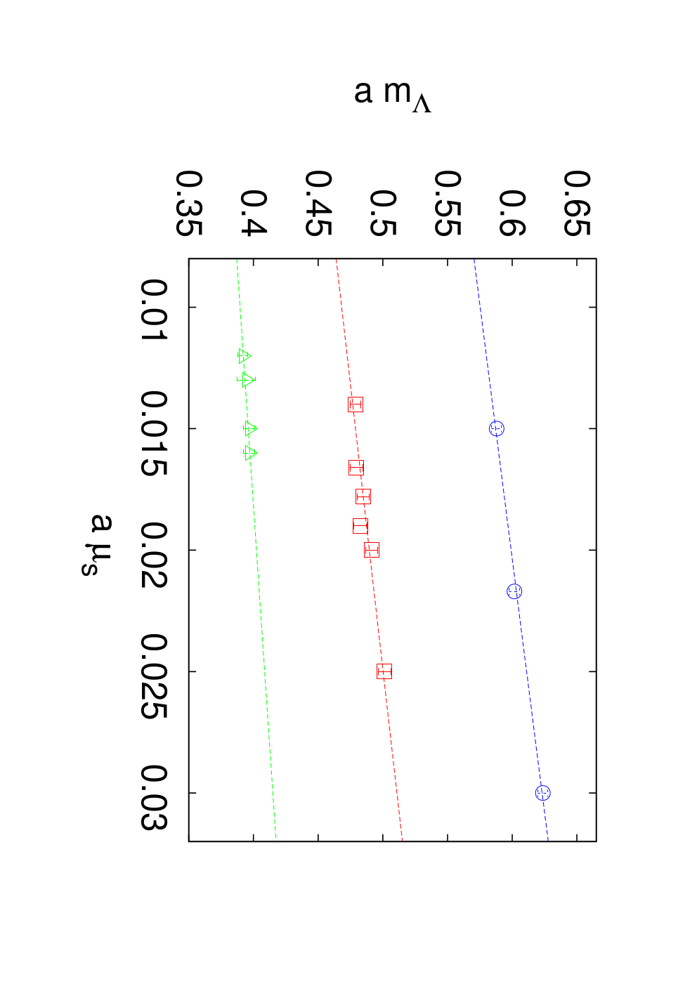
In Figs. 6 and 7 we show the dependence of the strange and charm baryon masses on the the strange and charm quark mass, respectively. Overall, the data display a linear dependence on both the strange and charm quark mass. One can therefore interpolate between different values of quark masses, if needed.
 |
 |
 |
 |
 |
 |
 |
 |
 |
 |
 |
 |
III.1 Strange baryon mass with strange quark mass tuned to its physical value
In this section we restrict our analysis only to the subset of data obtained at the tuned values of the strange quark mass. Namely, for and , we use the tuned value given in Table 3, whereas for we use which agrees with the tuned strange quark mass within error bars.


 |
 |
 |
 |
 |
 |
 |
 |
It is interesting to examine the degree of isospin splitting as a function of the lattice spacing. The splitting is expected to be zero in the continuum limit. In Fig. 8 we show the mass of , and at and 4.2. As expected the mass splitting among the three charge states of the decreases with the lattice spacing. The same behavior is observed for the other strange particles studied in this work. This is shown in Fig. 9 where we plot the mass difference as a function of at our smallest and heaviest pion mass. As can be seen, the mass difference is consistent with zero for all particles at the smallest lattice spacing. The small non-zero values seen for the and particles are just outside one standard deviation. Therefore, the general conclusion is that indeed isospin splitting is small at these values of the lattice spacing and it vanishes at the continuum limit. Since for finite there are small differnces, for the chiral extrapolation where we use all lattice data we do not average the masses for the different charge states of the , and .
Volume effects can be studied at where we have simulations at two volumes at pion mass of about 300 MeV. As can be seen in Figs. 8, 10 and 11 results at different volumes are consistent. Therefore, we conclude any volume effects are smaller than our statistical accuracy.
 |
 |
 |
 |
 |
 |
 |
 |
 |
 |
 |
 |
In order to examine the continuum limit we interpolate our lattice result at a given pion mass in units of . For we have simulations at only two values of the pion mass at the upper and lower range of pion masses considered in this work, namely for GeV and GeV. Therefore we interpolate the results for the other two values of to these two pion masses. In Figs. 10 and 11, we show results for the octet and decuplet strange baryon masses, respectively, at our three values of the lattice spacing. We perform a continuum extrapolation by perfroming a linear fit in as well as to constant. As can be seen from Fig. 10, the values obtained in the continuum limit agree for all octet baryons. In the case of the decuplet the statistical errors are larger and the value obtained at with the linear fit carries a large error. The value obtained using a constant fit has a smaller error and it is compatible with one the one obtained using a linear fit. Therefore, for a given charge state and within the current statistical accuracy, the term can be taken as negligible. Therefore, we can use results at all -values to extrapolate to the physical point since cut-off are small for a given charge state. There are two exceptions in the case of the decuplet. At the mass of the and at the lowest pion mass are systematically higher than that at the other two -values. Since the results at , with larger lattice space are consistent with those at we conclude that this is not a cut-off effect.
III.2 Charm baryon mass with charm quark mass tuned to its physical value
As in the previous subsection we consider results obtained at the tuned charm mass given in Table 3. The only exception is at at the heavy pion mass, where we have results close to the tuned value, namely at . As we have seen, the dependence on the heavy quark is linear and therefore the charm baryon masses at the tuned value can be easily determined by a linear interpolation.
 |
 |
 |
 |
 |
 |
 |
 |
 |
 |
 |
 |
 |
 |
 |
 |
 |
 |
 |
 |
We follow the same analysis as in the case of the strange baryon sector. In Fig. 12 we show the mass difference between different charged states as a function of the lattice spacing at the smallest and largest pion masses used in this work. As can be seen, the mass splittings are zero at the smallest value of the lattice spacing for all particles confirming restoration of isospin symmetry in the continuum limit. Furthermore, except for the case of the mass, the mass splitting is consistent with zero also at the other two -values. Therefore, for all particles except the one may average over the mass of different charge states.
In order to examine the continuum limit we interpolate our results at the three -values at a given pion mass in units of . In Figs. 13 and 14 we show the mass in the octet and decuplet charm sector as a function of lattice spacing for a given charge state, at the smallest and largest value of the pion mass. A linear fit in and a constant fit yield consistent results at the continuum limit, albeit with large errors in the case of th elinear fit. We also note that at the largest pion mass, although results at are in agreement with those at indicating neglegible -dependence, at the results are systematically below. We note that we show only statistical errors. Systematic errors due, for example, to the matching are not shown. As discussed in the next section these are (5-10)%. Therefore, a reasonable way to extrapolate our results in the charm sector is to compare the chiral extrapolation using all lattice data to those using results at and . We will take the different between the two values at the physical point as an estimate of a systematic error.
IV Chiral extrapolation
Having determined that effects are small for the lattice spacings considered here we can combine our lattice results at the various -values to extrapolate to the physical pion mass (physical point).
For the strange baryon sector, we consider SU(2) heavy baryon chiral perturbation, which was found to describe lattice data satisfactorily [2]. To leading one-loop one can described the pion mass dependence using
| (15) |
where is a known coefficient given in Ref. [2]. For completeness we give below the coefficients [35, 36]. For the octet baryons , and :
| (16) |
respectively, and for the decuplet baryons , and :
| (17) |
In addition we consider next to leading order SU(2) PT results [37]. The expressions are included here for completeness:
| (18) |
and for the decuplet baryons:
| (19) |
with the non analytic function [38]
| (20) |
depending on the threshold parameter and on the scale of chiral perturbation theory, fixed to GeV. For the real part of the function has the property
| (21) |
which corrects a typo in the sign of the second term in Ref. [5]. We follow the procedure of Ref. [2] and fix the nucleon axial charge and pion decay constant to their experimental values (we use the convention such that MeV). The remaining pion-baryon axial coupling constants are taken from SU(3) relations [37]. The fit parameters extracted for fitting to the NLO are given in Table 7. The deviation of the mean values obtained at the physical point when the results are fitted to leading order i.e. to Eq.( 15) with and when they are fitted to the NLO expressions provide an estimate of the systematic error due to the chiral extrapolation. We give this error in Table 7. In the case of the there is no difference between leading order and next to leading order. Since the contains three strange quarks any systematic error in the tuning of the strange quark mass will be largest in this case. Having results at several values of the strange quark mass we can estimate the change in the mass if the strange quark mass takes the maximum and minimum value allowed by the statistical error in the tuned strange quark mass. We take the difference in the mean values at the physical point obtained by varying the strange quark mas to be the systematic error due to the tuning. In Table 7 we give the systematic error on the mass of that we find following this procedure. This gives an upper bound of the error expected from the uncertainty in the tuning. As can be seen this is smaller as compared to the systematic error due to the chiral extrapolation and therefore it is only taken into account for the case of the .
| Particle(PDG) | (GeV) | (GeV-1) | d.o.f. | (GeV) |
|---|---|---|---|---|
| 1.1368(70) | 3.560(40) | 2.7 | 1.1930(62)(660) | |
| 1.3334(46) | 1.386(26) | 0.82 | 1.3538(41)(179) | |
| 1.0678(64) | 4.362(37) | 1.04 | 1.1276(57)(721) | |
| 1.4244(58) | 2.807(34) | 2.4 | 1.4757(51)(740) | |
| 1.4808(96) | 1.582(58) | 3.3 | 1.5113(89)(400) | |
| 1.7522(76) | 0.361(45) | 2.0 | 1.7591(67)(200) |
| Particle(PDG) | (GeV) | (GeV) |
|---|---|---|
| 2.494(47) | 0.143 | |
| 3.563(25) | 0.397 | |
| 2.229(43) | 0.223 | |
| 2.650(39) | 0.147 | |
| 3.672(42) | 0.274 | |
| 4.702(11) | 0.308 |
| Particle(PDG) | (GeV) | (GeV-1) | (GeV-2) | d.o.f. | (GeV) |
|---|---|---|---|---|---|
| 2.437(25) | 1.92(54) | -2.09(91) | 1.1 | 2.468(17)(23) | |
| 3.476(35) | 2.39(83) | -3.39(1.5) | 2.7 | 3.513(23)(14) | |
| 2.198(40) | 2.99(96) | -3.6(1.7) | 0.10 | 2.246(27)(15) | |
| 2.520(25) | 2.37(51) | -2.96(86) | 1.3 | 2.556(18)(51) | |
| 3.571(25) | 2.02(57) | -2.62(99) | 1.0 | 3.603(17)(21) | |
| 4.6706(53) | 0.327(35) | 0. | 2.5 | 4.6769(46)(30) |
In Figs. 10 and 11 we show the chiral extrapolation for the octet and the decuplet. In the case of the and the physical point is reproduced. However, for most other particles the lattice results extrapolate to a higher value. The worse deviation is seen for the . Since this has three strange quarks it may indicate that the tuning of the strange quark mass performed using the kaon mass introduces a systematic error. One can study partial quenching effects using twisted mass fermion simulations with a dynamical strange quark. This will be considered in a future study.
In the charm baryon sector we use the Ansatz
| (22) |
motivated by SU(2) HBPT to leading one-loop order, with taken as a fit parameter. For the we set since one does not expect a cubic term.
In order to assess the systematic error associated with the tuning of the charm quark mass we consider our results at . At this value of we have computed the charm baryon masses at the tuned value of the charm quark and at values of the charm quark shifted by the error on the tuned value. Since these computations were performed at four different light quark masses we can perform a chiral extrapolion using using the Ansatz of Eq. (22 for the set of masses obtained at the tuned value and at the value shifted by the error. The difference in the masses obtained at the physical pion mass is given in Tab. 8. As can be seen, this difference intorduces an error that varies between about 5% and 10%. This gives an estimate of the systemastic error due to the tuning of the charm quark mass. Since this analysis can only be done at we can only make a qualitative estimate of this error. Therefore in what follows we will not quote this error on our values,. However, one has to bear in mind that our final values can have a systematic error of about 10% due to the tunning.
In Figs. 13 and 14 we show fits at for our three values. We show fits using all data and fits using only data at and . The latter case yields a better fit with a smaller value of and this is the value quoted in Table 9. This is particularly noticeable for the case of where the results at are systematically lower. This maybe due to a small mismatch in the tuned value of the charm quark mass, which for the that contains three charm quarks would lead to the largest deviation. We take the difference in the extrapolated values at the physical points when we exclude the data from the fit as a systematic error.
The extrapolation of the lattice data reproduce the mass of experimentally measured charm baryon masses within a standard deviation, namely the mass of the , the and the . Therefore, the extrapolated lattice value can be taken as a prediction for the mass of the and the , within one standard deviation.
V Comparison with the results of other lattice formulations
In this section we compare our results with those using different discretization schemes by other collaborations. We also include a comparison for the nucleon and masses although they were not discussed in detail until now.
 |
 |
 |
 |
 |
 |
 |
 |

 |
 |
Several collaborations have calculated the strange baryon spectrum. The Budapest-Marseille-Wuppertal (BMW) collaboration carried out simulations using tree level improved 6-step stout smeared clover fermions and a tree level Symanzik improved gauge action. Volume effects were studied using lattices of spatial extent of 2 fm to 4.1 fm. The continuum limit was taken using results produced on three lattice spacings of fm, 0.085 fm and fm. Using pion masses down to 190 MeV a polynomial was performed to extrapolate to the physical value of the pion mass [4]. The PACS-CS collaboration obtained results using non-perturbatively improved clover fermions on an Iwasaki gauge action on a lattice of spatial length of 2.9 fm and lattice spacing fm [3]. The QCDSF-UKQCD collaboration [39] used Clover fermions with a single mild stout smearing and a lattice spacing fm. Finally, the LPHC collaboration [5] obtained results using a hybrid action of domain wall valence quarks on a staggered sea on lattice of spatial length 2.5 fm and 3.5 fm at lattice spacing fm.
In Fig. 15 we compare our results on the strange octet baryons with those from the BMW, the PACS-CS, the QCDSF-UKQCD and the LHPC collaborations. Our results and the results by the PACS-CS and LHPC are not continuum extrapolated. The BMW results are extrapolated to the continuum limit and have larger errors than the rest. Nevertheless, there is an overall agreement, indicating that cut-off effects are small. In Fig. 16 we compare our results on the strange decuplet baryons with the ones by PACS-CS and LHPC. Lattice results are in agreement except for the case of the where our results are consistently lower. Given the agreement of our results in the case of the this deviation cannot come from the mismatch in the strange quark mass. It is not clear what is the origin of this deviation for the , but the fact that the value obtained by PACS-CS at almost physical pion mass is high than the experimental value may indicate that the strange quark mass is larger than physical. In Fig. 17 we show the masses for the strange baryons after extrapolating to the physical pion mass. Fort the results of this work we plot the values extracted using NLO HBPT. Error shown on the twisted mass results is the estimate of the systematic error due to the chiral extrapolation, whereas the statistical errors are equal to the size of the symbols and are not shown. As can be seen, our results are in agreement with experiment except for , which is higher by 2%, just like the value found by PACS-CS.
We also compare in Fig. 18 our results for the charm baryons to those obtained using dynamical gauge configurations. All previous lattice computations of the mass of charm baryons used gauge configurations produced with staggered sea quarks with a number of different actions for the valence quarks. In Refs. [41, 42] a Clover charm valence quark was used on MILC gauge configurations at three values of the lattice spacing, fm. In Ref. [43] gauge configurations produced using the highly improved staggered quark (HISQ) action. The valence light-quark (up, down and strange) propagators are generated using the clover impoved Wilson action. In order to reduce discretization artifacts a relativistic heavy-quark action was adopted for the charm quark. Finally in Ref. [40] domain wall fermions are used for the up, the down and the strange quarks on improved Kogut-Susskind sea quarks at one value of the lattice spacing fm. The relativistic Fermilab action was employed for the charm quark. We show the comparison of our results to those obtained in the aforementioned references in Fig. 18. Our results for , , , , and are extrapolated to the physical pion mass using a polynomial fit with up -terms. For the spin 1/2 , , and we show the results obtained at MeV, the smallest value of the pion mass considered in this work on the lattice with the smallest lattice spacing at , for which cut-off effects are smallest. As can be seen, our results are in agreement with the results of the other studies except for the and with the experimental values. Although for we find a value consistent with the result of the SELEX experiment, one has to study the pion mass dependence in order to reach a final conclusion. In Fig. 18 we compare results for the spin 3/2 charm baryons. Our results for , and are obtained at MeV at . There is good agreement among lattice results and with the known experimental values for , and . Thus the lattice results can be taken as a prediction for the masses of the other charm spin 3/2 baryons shown in the figure.
VI Summary and Conclusions
In this work we have computed the strange and charm baryon masses using twisted mass fermions. For the strange and charm sector we use an Osterwalder-Seiler valence quarks. The bare strange and charm valence quark mass is tuned by requiring that the physical values of the mass of the kaon and D-meson are reproduced after the lattice results are extrapolated at the physical value of the pion mass.
We analyze gauge configurations for three values of the lattice spacings at the largest and smallest pion mass used in this study. We find that cut-off effects are small even in case of the charm baryons. This is a somewhat surprising result given that the Compton wave length of the D-meson mass is same order as the lattice spacing.
Using simulations on two different volumes we obtained results that are consistent showing that any volume effects are smaller than our statistical accuracy.
Another artifact of our lattice formulation is isospin breaking at finite lattice spacing. We have found that isospin breaking decreases with the lattice spacing and it is consistent with zero for fm confirming the expected restoration of isospin symmetry.
Our results on the strange quark sector are consistent with recent results using Clover improved fermions and domain wall fermions on a staggered sea. There is an overall agreement also in thee case of charm sector where we compare our results to other studies that used staggered sea quarks. The overall consistence among lattice results, despite the different discretizations used, provides a strong validation of lattice QCD computations. Our results on the charm baryons reproduce the experimentally known values and thus provide an estimate for the mass of the , , and .
Acknowledgments
We would like to thank all members of ETMC for a very constructive and enjoyable collaboration.
Numerical calculations have been performed at GENCI/IDRIS (Project i2011052271) and CC-IN2P3 computer centers. Computer time for this project was also made available to us by the John von Neumann-Institute for Computing on the Jugene BG/P system at the research center in Jülich and by the Computation-based Science and Technology Research Center of the Cyprus Institute through the infrastructure project Cy-Tera co-funded by the European Regional Development Fund and the Republic of Cyprus through the Research Promotion Foundation (Project Cy-Tera NEA YOOMH/TPATH/0308/31). This work was partly supported by funding received from the Cyprus Research Promotion Foundation under contracts PENEK/0609/17 and KY-A/0310/02. M.P. acknowledges financial support by the Marie Curie European Reintegration Grant of the 7th European Community Framework Programme under contract number PERG05-GA-2009-249309. M.G. was supported by the Marie-Curie European training network ITN STRONGnet grant PITN-GA-2009-238353.
References
- [1] C. Alexandrou et al. (European Twisted Mass Collaboration), Phys.Rev. D78, 014509 (2008), eprint 0803.3190.
- [2] C. Alexandrou et al. (ETM Collaboration), Phys.Rev. D80, 114503 (2009), eprint 0910.2419.
- [3] S. Aoki et al. (PACS-CS), Phys. Rev. D 79, 034503 (2009), eprint 0807.1661.
- [4] S. Durr et al., Science 322, 1224 (2008).
- [5] A. Walker-Loud, H.-W. Lin, D. Richards, R. Edwards, M. Engelhardt, et al., Phys.Rev. D79, 054502 (2009), eprint 0806.4549.
- [6] M. Mattson et al. (SELEX Collaboration), Phys.Rev.Lett. 89, 112001 (2002), eprint hep-ex/0208014.
- [7] J. Russ (SELEX Collaboration) (2002), eprint hep-ex/0209075.
- [8] A. Ocherashvili et al. (SELEX Collaboration), Phys.Lett. B628, 18 (2005), eprint hep-ex/0406033.
- [9] B. Aubert et al. (BABAR Collaboration), Phys.Rev. D74, 011103 (2006), eprint hep-ex/0605075.
- [10] S. Ratti, Nucl.Phys.Proc.Suppl. 115, 33 (2003).
- [11] R. Chistov et al. (BELLE Collaboration), Phys.Rev.Lett. 97, 162001 (2006), eprint hep-ex/0606051.
- [12] C. W. Bernard et al., Phys. Rev. D64, 054506 (2001), eprint hep-lat/0104002.
- [13] C. Aubin, C. Bernard, C. DeTar, J. Osborn, S. Gottlieb, et al., Phys.Rev. D70, 094505 (2004), eprint hep-lat/0402030.
- [14] A. Bazavov et al. (MILC collaboration), Phys.Rev. D82, 074501 (2010), eprint 1004.0342.
- [15] B. Blossier et al. (European Twisted Mass), JHEP 04, 020 (2008), eprint 0709.4574.
- [16] B. Blossier et al. (ETM Collaboration), JHEP 0907, 043 (2009), eprint 0904.0954.
- [17] P. Boucaud et al. (ETM), Phys. Lett. B650, 304 (2007), eprint hep-lat/0701012.
- [18] P. Boucaud et al. (ETM), Comput. Phys. Commun. 179, 695 (2008a), eprint 0803.0224.
- [19] R. Frezzotti and G. Rossi, PoS LAT2007, 277 (2007), eprint 0710.2492.
- [20] P. Dimopoulos et al. (ETM Collaboration), PoS LATTICE2008, 103 (2008), eprint 0810.2873.
- [21] K. Jansen, PoS LATTICE2008, 010 (2008), eprint 0810.5634.
- [22] P. Weisz, Nucl. Phys. B212, 1 (1983).
- [23] P. Boucaud et al. (2008b), eprint arXiv:0803.0224 [hep-lat].
- [24] R. Frezzotti, G. Martinelli, M. Papinutto, and G. Rossi, JHEP 0604, 038 (2006), eprint arXiv:hep-lat/0503034].
- [25] R. Frezzotti and G. Rossi, JHEP 0408, 007 (2004a).
- [26] R. Frezzotti and G. C. Rossi, JHEP 10, 070 (2004b), eprint hep-lat/0407002.
- [27] A. M. Abdel-Rehim, R. Lewis, R. M. Woloshyn, and J. M. S. Wu, Eur. Phys. J. A31, 773 (2007), eprint hep-lat/0610090.
- [28] A. M. Abdel-Rehim, R. Lewis, R. M. Woloshyn, and J. M. S. Wu, Phys. Rev. D74, 014507 (2006), eprint hep-lat/0601036.
- [29] C. Alexandrou et al. (ETM Collaboration), Phys.Rev. D83, 045010 (2011), eprint 1012.0857.
- [30] R. Baron et al. (ETM Collaboration), JHEP 1008, 097 (2010), eprint 0911.5061.
- [31] B. L. Ioffe, Nucl. Phys. B188, 317 (1981).
- [32] D. B. Leinweber, R. M. Woloshyn, and T. Draper, Phys. Rev. D43, 1659 (1991).
- [33] D. B. Leinweber, T. Draper, and R. M. Woloshyn, Phys. Rev. D46, 3067 (1992), eprint hep-lat/9208025.
- [34] U. Wolff (ALPHA), Comput. Phys. Commun. 156, 143 (2004), eprint hep-lat/0306017.
- [35] M. M. Nagels et al., Nucl. Phys. B147, 189 (1979a).
- [36] M. M. Nagels, T. A. Rijken, and J. J. de Swart, Phys. Rev. D20, 1633 (1979b).
- [37] B. C. Tiburzi and A. Walker-Loud, Phys. Lett. B669, 246 (2008), eprint 0808.0482.
- [38] B. C. Tiburzi and A. Walker-Loud, Nucl. Phys. A764, 274 (2006), eprint hep-lat/0501018.
- [39] W. Bietenholz, V. Bornyakov, M. Gockeler, R. Horsley, W. Lockhart, et al., Phys.Rev. D84, 054509 (2011), eprint 1102.5300.
- [40] L. Liu, H.-W. Lin, K. Orginos, and A. Walker-Loud, Phys.Rev. D81, 094505 (2010), eprint 0909.3294.
- [41] H. Na and S. A. Gottlieb, PoS LAT2007, 124 (2007), eprint 0710.1422.
- [42] H. Na and S. Gottlieb, PoS LATTICE2008, 119 (2008), eprint 0812.1235.
- [43] R. A. Briceno, D. Bolton, and H.-W. Lin (2011), eprint 1111.1028.
VII Appendix
In Tables 10, 11 and 12 the strange octet baryon masses are collected for , and , respectively. In Tables 13, 14 and 15 the strange decuplet baryon masses for the three beta are collected. In Tables 16, 17 and 18 we show the charm octet baryon masses for the three beta, while in Tables 19, 20 and 21 we show the charm decuplet baryon masses. In Table 22 we show the masses for extra spin-1/2 and spin-3/2 charm baryons at at the lightest pion mass we have.
| 32 | 0.0217 | 0.0030 | 0.597(3) | 0.577(4) | 0.607(7) | 0.657(4) | 0.628(3) | 0.561(3) |
|---|---|---|---|---|---|---|---|---|
| 24 | 0.0217 | 0.0040 | 0.610(5) | 0.600(3) | 0.622(4) | 0.671(3) | 0.638(2) | 0.577(4) |
| 32 | 0.0217 | 0.0040 | 0.616(4) | 0.596(5) | 0.628(7) | 0.675(4) | 0.635(3) | 0.574(4) |
| 24 | 0.0217 | 0.0064 | 0.628(5) | 0.610(6) | 0.640(9) | 0.687(5) | 0.650(4) | 0.602(4) |
| 24 | 0.0217 | 0.0085 | 0.649(3) | 0.631(2) | 0.668(4) | 0.697(3) | 0.659(2) | 0.619(3) |
| 24 | 0.0217 | 0.0100 | 0.654(4) | 0.643(5) | 0.666(6) | 0.696(5) | 0.668(3) | 0.633(4) |
| 24 | 0.015 | 0.0064 | 0.596(9) | 0.585(6) | 0.633(9) | 0.658(11) | 0.597(12) | 0.588(4) |
| 24 | 0.015 | 0.0085 | 0.641(5) | 0.598(11) | 0.663(6) | 0.674(5) | 0.621(6) | 0.594(9) |
| 24 | 0.015 | 0.0100 | 0.635(7) | 0.627(8) | 0.645(15) | 0.659(14) | 0.622(7) | 0.614(6) |
| 32 | 0.025 | 0.0040 | 0.623(5) | 0.606(5) | 0.633(9) | 0.687(6) | 0.651(4) | 0.587(8) |
| 32 | 0.030 | 0.0040 | 0.645(4) | 0.630(5) | 0.664(6) | 0.729(6) | 0.688(4) | 0.606(5) |
| 24 | 0.030 | 0.0064 | 0.654(5) | 0.640(6) | 0.674(7) | 0.732(5) | 0.682(7) | 0.624(4) |
| 24 | 0.030 | 0.0085 | 0.688(5) | 0.651(9) | 0.703(6) | 0.739(6) | 0.706(4) | 0.626(9) |
| 32 | 0.0178 | 0.0030 | 0.477(5) | 0.470(8) | 0.488(9) | 0.519(6) | 0.504(4) | 0.455(5) |
|---|---|---|---|---|---|---|---|---|
| 32 | 0.0178 | 0.0060 | 0.500(5) | 0.483(5) | 0.503(8) | 0.529(5) | 0.519(4) | 0.482(5) |
| 32 | 0.0178 | 0.0080 | 0.512(4) | 0.506(5) | 0.522(4) | 0.541(4) | 0.527(3) | 0.496(5) |
| 32 | 0.014 | 0.0030 | 0.463(5) | 0.456(9) | 0.474(9) | 0.496(6) | 0.482(4) | 0.445(6) |
| 32 | 0.014 | 0.0060 | 0.495(4) | 0.473(6) | 0.497(8) | 0.513(6) | 0.500(4) | 0.479(4) |
| 32 | 0.014 | 0.0080 | 0.494(8) | 0.508(9) | 0.508(5) | 0.512(7) | 0.507(3) | 0.485(6) |
| 32 | 0.0166 | 0.0030 | 0.477(5) | 0.465(5) | 0.487(6) | 0.515(4) | 0.498(3) | 0.451(4) |
| 32 | 0.0166 | 0.0060 | 0.496(5) | 0.483(5) | 0.502(5) | 0.526(4) | 0.511(4) | 0.480(5) |
| 32 | 0.0166 | 0.0080 | 0.510(3) | 0.502(3) | 0.518(4) | 0.535(3) | 0.521(3) | 0.496(3) |
| 32 | 0.019 | 0.0060 | 0.501(6) | 0.495(8) | 0.519(13) | 0.532(6) | 0.524(6) | 0.483(5) |
| 32 | 0.020 | 0.0030 | 0.486(6) | 0.478(8) | 0.495(8) | 0.531(6) | 0.517(4) | 0.461(5) |
| 32 | 0.020 | 0.0060 | 0.510(6) | 0.493(5) | 0.515(7) | 0.544(6) | 0.534(4) | 0.492(5) |
| 32 | 0.020 | 0.0080 | 0.516(4) | 0.510(7) | 0.514(7) | 0.547(4) | 0.533(4) | 0.500(5) |
| 32 | 0.025 | 0.0060 | 0.522(5) | 0.501(6) | 0.531(7) | 0.572(5) | 0.556(4) | 0.501(5) |
| 32 | 0.012 | 0.0065 | 0.402(4) | 0.396(4) | 0.405(5) | 0.418(4) | 0.406(4) | 0.392(4) |
|---|---|---|---|---|---|---|---|---|
| 48 | 0.012 | 0.0020 | 0.362(3) | 0.360(3) | 0.368(4) | 0.390(2) | 0.381(2) | 0.344(3) |
| 32 | 0.013 | 0.0065 | 0.406(7) | 0.405(7) | 0.417(7) | 0.430(6) | 0.416(6) | 0.395(7) |
| 32 | 0.015 | 0.0065 | 0.411(4) | 0.409(4) | 0.413(4) | 0.431(4) | 0.421(4) | 0.397(4) |
| 48 | 0.015 | 0.0020 | 0.374(2) | 0.371(3) | 0.380(3) | 0.404(2) | 0.397(2) | 0.352(2) |
| 32 | 0.016 | 0.0065 | 0.417(7) | 0.409(4) | 0.413(4) | 0.442(5) | 0.421(4) | 0.397(4) |
| 32 | 0.0217 | 0.0030 | 0.700(7) | 0.713(5) | 0.700(6) | 0.710(6) | 0.702(5) | 0.798(3) |
|---|---|---|---|---|---|---|---|---|
| 32 | 0.0217 | 0.0040 | 0.726(4) | 0.718(6) | 0.715(6) | 0.739(4) | 0.721(4) | 0.809(3) |
| 24 | 0.0217 | 0.0040 | 0.716(12) | 0.726(14) | 0.717(17) | 0.737(8) | 0.714(8) | 0.805(7) |
| 24 | 0.0217 | 0.0064 | 0.749(7) | 0.749(7) | 0.740(11) | 0.754(8) | 0.734(8) | 0.815(6) |
| 24 | 0.0217 | 0.0085 | 0.759(5) | 0.755(4) | 0.755(5) | 0.767(3) | 0.738(5) | 0.820(3) |
| 24 | 0.0217 | 0.0100 | 0.773(8) | 0.772(8) | 0.773(9) | 0.784(5) | 0.749(7) | 0.834(4) |
| 24 | 0.015 | 0.0064 | 0.737(24) | 0.736(7) | 0.746(7) | 0.728(15) | 0.708(10) | 0.772(16) |
| 24 | 0.015 | 0.0085 | 0.751(10) | 0.736(20) | 0.755(7) | 0.723(11) | 0.659(18) | 0.771(9) |
| 24 | 0.015 | 0.0100 | 0.730(18) | 0.757(19) | 0.746(16) | 0.720(15) | 0.667(10) | 0.771(11) |
| 32 | 0.025 | 0.0040 | 0.730(9) | 0.723(12) | 0.710(14) | 0.747(12) | 0.738(8) | 0.827(7) |
| 32 | 0.030 | 0.0040 | 0.724(11) | 0.743(10) | 0.739(9) | 0.782(7) | 0.765(8) | 0.870(6) |
| 24 | 0.030 | 0.0064 | 0.772(6) | 0.769(6) | 0.760(11) | 0.797(7) | 0.781(6) | 0.874(6) |
| 24 | 0.030 | 0.0085 | 0.782(11) | 0.736(7) | 0.746(7) | 0.812(7) | 0.751(11) | 0.771(9) |
| 32 | 0.0178 | 0.0030 | 0.597(11) | 0.589(10) | 0.590(13) | 0.596(8) | 0.588(6) | 0.661(7) |
|---|---|---|---|---|---|---|---|---|
| 32 | 0.0178 | 0.0060 | 0.593(8) | 0.586(8) | 0.582(8) | 0.582(7) | 0.583(7) | 0.638(6) |
| 32 | 0.0178 | 0.0080 | 0.606(6) | 0.607(7) | 0.606(6) | 0.609(6) | 0.598(5) | 0.651(6) |
| 32 | 0.014 | 0.0030 | 0.589(12) | 0.595(8) | 0.603(6) | 0.578(8) | 0.570(6) | 0.627(8) |
| 32 | 0.014 | 0.0060 | 0.586(11) | 0.574(13) | 0.582(12) | 0.568(10) | 0.559(11) | 0.623(7) |
| 32 | 0.014 | 0.0080 | 0.588(10) | 0.606(7) | 0.592(6) | 0.574(9) | 0.574(6) | 0.614(8) |
| 32 | 0.0166 | 0.0030 | 0.570(12) | 0.578(7) | 0.561(8) | 0.573(6) | 0.567(6) | 0.630(5) |
| 32 | 0.0166 | 0.0060 | 0.582(12) | 0.578(10) | 0.568(14) | 0.579(6) | 0.577(7) | 0.622(8) |
| 32 | 0.0166 | 0.0080 | 0.615(4) | 0.609(6) | 0.604(7) | 0.601(5) | 0.586(5) | 0.648(4) |
| 32 | 0.019 | 0.0060 | 0.592(16) | 0.576(13) | 0.551(19) | 0.579(8) | 0.583(9) | 0.648(5) |
| 32 | 0.020 | 0.0030 | 0.611(7) | 0.605(8) | 0.610(7) | 0.606(7) | 0.596(8) | 0.671(5) |
| 32 | 0.020 | 0.0060 | 0.599(10) | 0.591(9) | 0.595(11) | 0.594(11) | 0.591(9) | 0.657(6) |
| 32 | 0.020 | 0.0080 | 0.610(6) | 0.619(6) | 0.605(6) | 0.613(8) | 0.597(6) | 0.660(5) |
| 32 | 0.025 | 0.0060 | 0.598(11) | 0.589(12) | 0.577(15) | 0.613(7) | 0.613(8) | 0.674(8) |
| 32 | 0.012 | 0.0065 | 0.480(7) | 0.482(6) | 0.476(8) | 0.468(6) | 0.464(6) | 0.498(6) |
|---|---|---|---|---|---|---|---|---|
| 48 | 0.012 | 0.0020 | 0.453(4) | 0.451(4) | 0.451(4) | 0.444(3) | 0.440(3) | 0.487(3) |
| 32 | 0.013 | 0.0065 | 0.501(11) | 0.500(10) | 0.495(14) | 0.494(9) | 0.489(9) | 0.522(10) |
| 32 | 0.015 | 0.0065 | 0.478(6) | 0.487(5) | 0.477(6) | 0.478(5) | 0.475(5) | 0.513(4) |
| 48 | 0.015 | 0.0020 | 0.458(4) | 0.455(3) | 0.452(2) | 0.440(4) | 0.448(4) | 0.505(3) |
| 32 | 0.016 | 0.0065 | 0.507(11) | 0.487(5) | 0.503(12) | 0.504(10) | 0.505(9) | 0.540(10) |
| 24 | 0.240 | 0.0040 | 1.100(6) | 1.105(13) | 1.102(14) | 1.532(5) | 1.528(4) | 1.015(8) |
|---|---|---|---|---|---|---|---|---|
| 24 | 0.240 | 0.0064 | 1.117(6) | 1.059(20) | 1.122(6) | 1.552(3) | 1.533(4) | 1.045(5) |
| 24 | 0.240 | 0.0085 | 1.131(6) | 1.125(5) | 1.135(5) | 1.555(4) | 1.541(5) | 1.063(3) |
| 24 | 0.240 | 0.0100 | 1.139(4) | 1.131(5) | 1.138(5) | 1.559(3) | 1.551(2) | 1.070(3) |
| 24 | 0.250 | 0.0040 | 1.128(7) | 1.120(9) | 1.099(14) | 1.591(5) | 1.575(5) | 1.055(6) |
| 24 | 0.270 | 0.0040 | 1.154(5) | 1.157(5) | 1.161(6) | 1.640(4) | 1.628(3) | 1.069(4) |
| 24 | 0.270 | 0.0064 | 1.172(7) | 1.164(5) | 1.176(7) | 1.648(5) | 1.634(4) | 1.096(5) |
| 24 | 0.270 | 0.0085 | 1.192(4) | 1.181(4) | 1.188(5) | 1.658(3) | 1.651(3) | 1.115(3) |
| 24 | 0.270 | 0.0100 | 1.196(4) | 1.189(4) | 1.197(4) | 1.660(3) | 1.649(25) | 1.122(3) |
| 24 | 0.300 | 0.0040 | 1.203(9) | 1.214(5) | 1.221(5) | 1.736(6) | 1.731(4) | 1.135(4) |
| 24 | 0.300 | 0.0064 | 1.227(4) | 1.162(22) | 1.236(5) | 1.747(4) | 1.722(6) | 1.148(5) |
| 24 | 0.300 | 0.0085 | 1.244(4) | 1.236(4) | 1.244(4) | 1.759(3) | 1.736(6) | 1.169(3) |
| 24 | 0.300 | 0.0100 | 1.251(3) | 1.237(5) | 1.249(4) | 1.762(2) | 1.751(3) | 1.172(3) |
| 32 | 0.170 | 0.0030 | 0.843(4) | 0.841(5) | 0.839(6) | 1.134(5) | 1.137(4) | 0.774(5) |
|---|---|---|---|---|---|---|---|---|
| 32 | 0.170 | 0.0060 | 0.844(4) | 0.831(9) | 0.836(8) | 1.149(3) | 1.139(4) | 0.791(5) |
| 32 | 0.170 | 0.0080 | 0.852(4) | 0.852(5) | 0.852(7) | 1.146(2) | 1.142(3) | 0.791(6) |
| 32 | 0.200 | 0.0030 | 0.900(4) | 0.888(7) | 0.894(6) | 1.244(3) | 1.244(5) | 0.828(6) |
| 32 | 0.200 | 0.0060 | 0.903(4) | 0.886(10) | 0.891(8) | 1.255(2) | 1.250(3) | 0.843(5) |
| 32 | 0.200 | 0.0080 | 0.905(5) | 0.907(5) | 0.908(8) | 1.250(2) | 1.247(3) | 0.848(5) |
| 32 | 0.210 | 0.0030 | 0.917(4) | 0.912(6) | 0.908(7) | 1.282(3) | 1.276(4) | 0.845(6) |
| 32 | 0.210 | 0.0060 | 0.919(4) | 0.911(4) | 0.921(4) | 1.286(3) | 1.279(3) | 0.859(5) |
| 32 | 0.210 | 0.0080 | 0.926(3) | 0.925(4) | 0.926(4) | 1.288(2) | 1.283(2) | 0.865(4) |
| 32 | 0.230 | 0.0030 | 0.952(5) | 0.942(7) | 0.948(6) | 1.345(3) | 1.342(5) | 0.883(5) |
| 32 | 0.230 | 0.0060 | 0.952(4) | 0.940(11) | 0.945(8) | 1.355(3) | 1.353(3) | 0.895(5) |
| 32 | 0.230 | 0.0080 | 0.959(5) | 0.960(5) | 0.959(5) | 1.349(3) | 1.349(3) | 0.899(5) |
| 32 | 0.260 | 0.0030 | 1.004(5) | 1.005(10) | 1.003(5) | 1.444(3) | 1.441(5) | 0.935(5) |
| 32 | 0.260 | 0.0060 | 1.001(5) | 0.992(11) | 0.997(8) | 1.457(3) | 1.451(4) | 0.946(5) |
| 32 | 0.260 | 0.0080 | 1.010(6) | 1.011(7) | 1.012(8) | 1.449(3) | 1.446(5) | 0.955(3) |
| 32 | 0.130 | 0.0065 | 0.696(6) | 0.694(6) | 0.698(6) | 0.932(4) | 0.927(5) | 0.653(4) |
|---|---|---|---|---|---|---|---|---|
| 32 | 0.160 | 0.0065 | 0.733(6) | 0.731(6) | 0.734(7) | 0.999(4) | 0.997(5) | 0.688(4) |
| 32 | 0.185 | 0.0065 | 0.778(7) | 0.776(6) | 0.779(7) | 1.085(4) | 1.082(5) | 0.731(4) |
| 32 | 0.210 | 0.0065 | 0.821(7) | 0.819(7) | 0.822(7) | 1.168(4) | 1.156(5) | 0.774(4) |
| 48 | 0.136 | 0.0020 | 0.653(3) | 0.656(3) | 0.652(3) | 0.899(2) | 0.898(2) | 0.603(2) |
| 48 | 0.170 | 0.0020 | 0.716(3) | 0.719(3) | 0.715(4) | 1.017(2) | 1.016(2) | 0.663(3) |
| 24 | 0.240 | 0.0040 | 1.148(10) | 1.142(16) | 1.147(15) | 1.572(6) | 1.564(6) | 1.989(3) |
|---|---|---|---|---|---|---|---|---|
| 24 | 0.240 | 0.0064 | 1.159(10) | 1.151(9) | 1.166(11) | 1.580(6) | 1.572(5) | 1.991(4) |
| 24 | 0.240 | 0.0085 | 1.175(8) | 1.164(8) | 1.174(10) | 1.594(5) | 1.578(7) | 1.997(4) |
| 24 | 0.240 | 0.0100 | 1.184(6) | 1.184(4) | 1.181(6) | 1.599(3) | 1.591(3) | 1.999(3) |
| 24 | 0.250 | 0.0040 | 1.173(8) | 1.182(9) | 1.173(11) | 1.602(7) | 1.606(8) | 2.043(4) |
| 24 | 0.270 | 0.0040 | 1.201(8) | 1.204(7) | 1.210(5) | 1.671(7) | 1.668(5) | 2.130(3) |
| 24 | 0.270 | 0.0064 | 1.209(10) | 1.210(5) | 1.225(6) | 1.680(5) | 1.672(5) | 2.133(3) |
| 24 | 0.270 | 0.0085 | 1.231(4) | 1.224(5) | 1.230(4) | 1.692(5) | 1.686(3) | 2.136(4) |
| 24 | 0.270 | 0.0100 | 1.239(4) | 1.234(4) | 1.238(5) | 1.694(4) | 1.690(4) | 2.141(3) |
| 24 | 0.300 | 0.0040 | 1.263(5) | 1.245(15) | 1.260(6) | 1.775(6) | 1.764(5) | 2.269(3) |
| 24 | 0.300 | 0.0064 | 1.267(5) | 1.260(5) | 1.275(6) | 1.779(5) | 1.768(5) | 2.270(3) |
| 24 | 0.300 | 0.0085 | 1.281(4) | 1.274(5) | 1.280(4) | 1.794(3) | 1.770(8) | 2.274(4) |
| 24 | 0.300 | 0.0100 | 1.292(3) | 1.283(4) | 1.282(6) | 1.795(3) | 1.789(3) | 2.277(2) |
| 32 | 0.170 | 0.0030 | 0.889(6) | 0.889(6) | 0.890(4) | 1.170(6) | 1.174(5) | 1.468(3) |
|---|---|---|---|---|---|---|---|---|
| 32 | 0.170 | 0.0060 | 0.887(4) | 0.883(5) | 0.868(12) | 1.184(3) | 1.172(6) | 1.476(2) |
| 32 | 0.170 | 0.0080 | 0.885(5) | 0.890(7) | 0.884(5) | 1.176(3) | 1.175(4) | 1.468(3) |
| 32 | 0.200 | 0.0030 | 0.940(6) | 0.940(6) | 0.941(4) | 1.277(4) | 1.281(4) | 1.616(3) |
| 32 | 0.200 | 0.0060 | 0.928(6) | 0.937(4) | 0.918(11) | 1.288(3) | 1.281(3) | 1.623(2) |
| 32 | 0.200 | 0.0080 | 0.936(5) | 0.945(6) | 0.935(5) | 1.279(3) | 1.281(3) | 1.612(3) |
| 32 | 0.210 | 0.0030 | 0.956(6) | 0.956(6) | 0.958(4) | 1.310(4) | 1.314(4) | 1.663(3) |
| 32 | 0.210 | 0.0060 | 0.955(5) | 0.954(4) | 0.948(5) | 1.316(3) | 1.310(4) | 1.667(2) |
| 32 | 0.210 | 0.0080 | 0.957(4) | 0.962(4) | 0.958(4) | 1.316(3) | 1.313(3) | 1.663(3) |
| 32 | 0.230 | 0.0030 | 0.989(6) | 0.989(6) | 0.992(4) | 1.376(4) | 1.379(4) | 1.761(3) |
| 32 | 0.230 | 0.0060 | 0.984(4) | 0.987(4) | 0.967(11) | 1.387(3) | 1.380(4) | 1.768(2) |
| 32 | 0.230 | 0.0080 | 0.986(5) | 0.995(6) | 0.986(5) | 1.378(3) | 1.380(3) | 1.758(3) |
| 32 | 0.260 | 0.0030 | 1.039(6) | 1.038(6) | 1.036(7) | 1.473(4) | 1.476(4) | 1.905(3) |
| 32 | 0.260 | 0.0060 | 1.033(5) | 1.032(5) | 1.016(11) | 1.485(3) | 1.478(4) | 1.910(3) |
| 32 | 0.260 | 0.0080 | 1.034(5) | 1.039(6) | 1.032(10) | 1.472(3) | 1.472(5) | 1.898(4) |
| 32 | 0.130 | 0.0065 | 0.730(8) | 0.730(8) | 0.727(8) | 0.958(6) | 0.963(6) | 1.191(3) |
|---|---|---|---|---|---|---|---|---|
| 32 | 0.160 | 0.0065 | 0.763(8) | 0.763(8) | 0.761(8) | 1.025(6) | 1.029(6) | 1.287(3) |
| 32 | 0.185 | 0.0065 | 0.805(8) | 0.804(8) | 0.802(8) | 1.107(6) | 1.109(6) | 1.408(3) |
| 32 | 0.210 | 0.0065 | 0.845(9) | 0.845(8) | 0.843(8) | 1.188(6) | 1.193(6) | 1.526(3) |
| 48 | 0.136 | 0.0020 | 0.686(4) | 0.688(3) | 0.683(4) | 0.925(2) | 0.926(2) | 1.166(1) |
| 48 | 0.170 | 0.0020 | 0.744(4) | 0.746(3) | 0.741(4) | 1.039(2) | 1.039(2) | 1.333(1) |
| 48 | 0.015 | 0.17 | 0.0020 | 0.708(2) | 0.745(3) | 0.771(2) | 1.044(1) | 0.770(3) | 0.794(2) | 1.065(2) |
|---|