Search for a T-odd, P-even Triple Correlation in Neutron Decay
Abstract
Background: Time-reversal-invariance violation, or equivalently CP violation, may explain the observed cosmological baryon asymmetry as well as signal physics beyond the Standard Model. In the decay of polarized neutrons, the triple correlation is a parity-even, time-reversal-odd observable that is uniquely sensitive to the relative phase of the axial-vector amplitude with respect to the vector amplitude. The triple correlation is also sensitive to possible contributions from scalar and tensor amplitudes. Final-state effects also contribute to at the level of 10-5 and can be calculated with a precision of 1% or better. Purpose: We have improved the sensitivity to T-odd, P-even interactions in nuclear beta decay. Methods: We measured proton-electron coincidences from decays of longitudinally polarized neutrons with a highly symmetric detector array designed to cancel the time-reversal-even, parity-odd Standard-Model contributions to polarized neutron decay. Over 300 million proton-electron coincidence events were used to extract and study systematic effects in a blind analysis. Results: We find . Conclusions: This is the most sensitive measurement of in nuclear beta decay. Our result can be interpreted as a measurement of the phase of the ratio of the axial-vector and vector coupling constants ( ) with (68% confidence level) or to constrain time-reversal violating scalar and tensor interactions that arise in certain extensions to the Standard Model such as leptoquarks. This paper presents details of the experiment, analysis, and systematic-error corrections.
pacs
24.80.+y, 11.30.Er, 12.15.Ji, 13.30.CeI Introduction
The symmetries of physical processes under the transformations of charge conjugation (C), parity (P), and time reversal (T) have played a central role in the development of the Standard Model of elementary-particle interactions [1]. Time-reversal-symmetry violation (or T violation), which is equivalent to CP violation assuming CPT symmetry, has been of particular interest because it is sensitive to many kinds of new physics. The CP-violating parameters of the Standard Model are the Cabibbo-Kobayashi-Maskawa (CKM) phase, which enters in the mixing of three generations of quarks, and the parameter . The effect of the CKM phase is strongly suppressed in the permanent electric dipole moments (EDMs) of the neutron [2] and heavy atoms [3, 4], and recent EDM results combine to set upper limits on . All laboratory measurements to date are consistent with a single source of CP violation, i.e. the phase in the CKM matrix. An exception may be the 3.2 sigma deviation observed recently as an asymmetry in the production of pairs of like-sign muons reported by the D0 collaboration [5].
In spite of this success, laboratory and astrophysical observations, which include neutrinos with non-zero masses, the abundance of non-baryonic dark matter, and the baryon asymmetry of the universe, provide strong evidence that the Standard Model is incomplete. Generation of the baryon asymmetry requires CP violation that cannot be accounted for by Standard-Model physics [6, 7]. This provides strong motivation to search for new sources of CP violation. Such CP-violating phases would also, in general, affect T-odd observables in neutron decay, in particular, the T-odd/P-even triple correlation in polarized neutron decay.
We have measured the triple-correlation in the decay of polarized neutrons at the NIST Center for Neutron Research (NCNR) using the emiT apparatus [8, 9, 10]. The -coefficient is uniquely sensitive to the relative phase of vector and axial vector amplitudes and is also sensitive to scalar and tensor currents. Our result, first reported in reference [11], sets a new limit on this phase as well as on certain combinations of scalar and tensor currents.
This paper presents the details of the experiment and analysis and examines the implications of this result. The paper is organized as follows: The context of the measurement is presented in the remainder of this introduction. In section II the measurement principle based on the symmetries of the apparatus is presented. The Monte Carlo simulations used to understand the apparatus and important details of the performance of the apparatus are provided in sections III and IV. In section V we present the details of the data set; and section VI is a detailed discussion of all systematic effects and corrections applied to the data. In section VII we describe the principle of the blind analysis and present the final result; and in section VIII we summarize the implications of our result and prospects for improved measurements.
I.1 Polarized neutron decay
Neglecting recoil-order corrections, the general form of the Hamiltonian for beta-decay (e.g. ) can be written [12]
| (1) | |||||
where the subscripts , , , and respectively refer to vector, axial-vector, scalar, and tensor contributions, and we have left out the pseudoscalar amplitude, which vanishes in the limit of non-relativistic nucleons. Allowing the possibility of T violation, the ’s are complex numbers, and there are 19 free parameters plus a single arbitrary overall phase. The Standard Model is written with only left-handed and interactions with and . Thus the number of free parameters is reduced to three: , and the relative phase of . The value of follows from the conserved-vector-current hypothesis (CVC) with determined from the muon lifetime, and most precisely determined from super-allowed beta decays [13]. The parameter is determined from other measurements including the beta asymmetry (-term) and electron-neutrino correlation (-term).
The Hamiltonian of Eq. 1 leads to the following differential decay rate for polarized neutrons and no final-state electron polarization [12]:
| (2) |
where is the phase space factor with the Fermi-function for , and are the momentum(energy) of the electron and antineutrino, and the neutron polarization is the ensemble average of the neutron spin. The triple-correlation, is P-even but odd under motion reversal. Time-reversal is the combination of motion-reversal and initial/final-state reversal. Thus contributions to can originate from T-violating interactions and from final state effects, i.e. [14], where
| (3) |
For the neutron and can be calculated to 1% or better [15, 16, 17].
In the neutron rest frame, (for cold neutrons, the neutron velocity in the lab frame has a negligible effect), and the triple correlation can be written
| (4) |
We therefore extract by measuring proton-electron angular correlations in polarized-neutron decay.
I.2 The Physics of
In the context of Eq. 1, depends on the values of and can be written as [15]
where and are matrix elements for Fermi and Gamow-Teller transitions (for neutrons, ), and
| (6) | |||||
We assume terms quadratic in and can be neglected in , and take and (i.e. left-handed - interactions) so that
| (7) |
where . The first term is sensitive to the phase of and can be approximately written for [24]. The remaining terms show sensitivity to combinations of scalar and tensor amplitudes that signal beyond-Standard-Model Physics.
Standard-Model CP violation makes very small contributions to . The CKM phase enters light-quark processes at loop level yielding [28, 29]. The parameter is tightly constrained by the EDMs of the neutron and 199Hg and also makes a very small contribution to , i.e. less than [28, 29]. Beyond-Standard-Model physics, in particular left-right symmetric models, exotic fermions, and leptoquarks give rise to couplings that contribute to at a level comparable to the current experimental sensitivity; however, it has been argued that limits on T-odd/P-odd observables, in particular EDMs, can be used to place limits on T-odd/P-even interactions and thus on by calculating the T-odd/P-even effects of radiative loops on T-odd/P-odd interactions [18, 19, 20, 21, 22]. For the neutron EDM, this limit is more stringent than the sensitivity of the experiment described here by as much as an order of magnitude; however, this argument is based on the assumption of complete absence of cancellations between different contributions to the neutron EDM, which cannot be a priori excluded [22]. Table 1 summarizes the contributions to from the Standard Model and extensions.
| Model/Parameter | Limit on |
|---|---|
| CKM phase | |
| Left-right symmetry | -10-5 |
| Non-SM fermions | -10-5 |
| Charged Higgs SUSY | -10-6 |
| Leptoquark | 10-5-10-4 |
I.3 Recent results
The two most recent measurements of in neutron decay are the emiT-I measurement and the TRINE experiment result from Institute Laue Langevin, Grenoble (ILL). For emiT-I, [9], and the TRINE result was [23]. The current Particle Data Group average for the neutron, [24], also includes results from references [25, 26, 27]. A measurement in 19Ne, where the final-state-interactions are more than an order of magnitude larger than for the neutron, resulted in [30, 31]. We also note that the coefficient of the T-odd/P-odd correlation , which is linearly sensitive to S and T amplitudes, has recently been measured for the neutron [32] and for 8Li [33].
II The emiT-II experiment
The emiT experiment was designed to measure proton-electron coincidences in the decay of neutrons polarized along the axis of an array of detectors. The symmetry of the detector array allowed us to discriminate the triple correlation from the T-even/P-odd - and -coefficient correlations. The layout of the experiment is shown in Fig. 1. The cold neutron beam was transported by the neutron guide NG6 to the experiment. The neutrons were polarized and passed through a spin flipper. Downstream of the spin-flipper, neutron spins were adiabatically transported through rotation of the magnetic field to longitudinal, along the axis of the detector array.
The detector array, illustrated in Fig. 2, consists of four electron-detectors alternating with four proton-detector planes arranged in an octagonal geometry concentric with the neutron beam. Each of the four proton-detector planes consists of 16 separate cells arranged in two rows of eight cells. The protons are detected by negatively-biased surface barrier detectors (SBDs) that are incorporated into a focusing cell illustrated in Fig. 3. Within the fiducial volume of the detector array, neutrons are polarized parallel or antiparallel to the magnetic field depending on the state of the spin flipper. The magnetic field in the detector region is approximately 560 T in magnitude and is aligned parallel to the neutron beam and detector axis.

II.1 Electron-proton Coincidence Events
The data set consists of 512 sets of coincidence events from the combination of 64 proton cells and four electron detectors for the two spin-flipper states. The total number of counts for a given run time is labeled as , where the indicates the spin-flipper state (neutrons nominally parallel/opposite to the magnetic field ), labels the proton-cell, and labels the electron detector. The neutron-spin dependence of the count rates depends on the correlations given by , , and and is given by the difference of rates for the two spin-flipper states, while the average of rates includes the spin-independent beta-neutrino correlation ( term).
In order to isolate the neutron-spin dependent terms, we define the asymmetry
| (8) |
In principle, the follow from integrating Eq. 2 over the neutron beam, the detectors’ acceptances, electron momentum, and neutrino angles for a fixed time so that
| (9) |
where is the electron velocity, is the neutron polarization at a given position, and the brackets () indicate that each term is integrated over energies, the neutron-beam distribution, and solid angles for proton detector and electron detector . As shown below, the -coefficient term can be isolated by forming a specific combination of that cancels the parity-violating and correlations.
II.2 The ideal experiment
In order to understand the analysis technique, we begin by considering an ideal experiment with uniform longitudinal neutron polarization (), uniform neutron-beam density, and uniform efficiencies for all proton and electron detectors. Consider a proton detected in in coincidence with an electron detected in either detector or as shown in Fig. 2. (Coincidence rates of with and were about 15-25 times lower and were not used to extract in this analysis.) Thus, for longitudinal neutron polarization, the asymmetry from Eq. 9 can be written
| (10) |
where and are the polar angles of the electron and antineutrino with respect to the neutron polarization , and
It is useful to define an instrumental constant that characterizes the sensitivity of to the triple correlation, i.e. or
| (11) |
The used in the analysis were determined by Monte Carlo studies and are discussed in section VI.6.
In order to isolate the triple correlation, we note that the longitudinal component of the cross product, , has opposite sign for and coincidences: for , it is positive, and for , it is negative. Thus we form a difference of spin-flip asymmetries for the two electron detectors. For example, for we have: . Using Eq. 10, the for longitudinal polarization are
| (12) | |||||
where . Due to strong anti-correlation of proton and electron momenta, the asymmetries depend strongly on the axial position of the proton cell. (Data are shown in Figs. 12 and 13.) For example, assuming , the (and ) are equal but opposite for the upstream proton cell and an axially symmetric downstream proton cell for a uniform neutron beam, e.g. . Also note that in the absence of the 560 T magnetic field, the are opposite for the adjacent proton cell, e.g. . Thus, for an ideal experiment with uniform longitudinal polarization and beam, the average of from an upstream-downstream pair of proton cells (e.g. and ) or adjacent cells (e.g. and ) will cancel the beta-asymmetry and neutrino-asymmetry terms leaving the -coefficient term; however, the magnetic field affects the average differently for odd (e.g. ) and even (e.g. ) proton detectors. Thus we combine data for all four proton cells in order to isolate .
Transverse neutron polarization
A small misalignment of the magnetic field with respect to the detector axis gives rise to transverse-polarization effects. In the limit of a small beam diameter and a small angular acceptance of the proton cell, the average proton momentum is the same for the two electron detectors (e.g. and ), and for transverse polarization, indicated by the subscript , we can write
| (13) |
where is the azimuthal angle of the polarization, is the effective azimuthal position of the proton cell as indicated in Fig. 2, and . The factor 0.46 is consistent with both Monte-Carlo simulations and the transverse-polarization calibration runs discussed in section VI.5. Thus, for uniform neutron density and polarization, the sinusoidal dependence of on the azimuthal position of the proton-cell averages to zero when data from all four proton-detector planes are combined.
Extracting
In order to cancel the effects of transverse polarization, the beta and neutrino asymmetries, and the 560 T magnetic field, we must combine the from at least 16 proton cells symmetrically located with respect to the center of the detector: two adjacent cells upstream of the detector center paired with two adjacent downstream cells from all four proton planes. Each set of 16 proton cells have the same , i.e. = 2 , 6, 10, and 14 cm. For example, the shaded detectors in Fig. 2 correspond to cm. For each we define a measured quantity given by
| (14) |
where is discussed in section VI.6. Due to the symmetry with respect to the detector center, each of the four possible is an independent measurement of the same nominal quantity. This provides cross checks and maximum statistical power. The are subject to a variety of systematic effects that are estimated and applied as corrections in order to determine . Corrections to are discussed in section VI.
III Monte Carlo simulations
Monte Carlo simulations were used both in the design of the experiment and to estimate several of the systematic effects that impact the analysis. Separate simulations addressed the detector responses, proton focusing cells, and neutron spin transport.
To track electrons, we used penelope [34], which has been experimentally validated for a variety of kinematics of relevance to neutron decay [35]. To track protons we used custom code embedded into penelope. The Monte Carlo code used the measured beam distributions and took into account the 560 T axial magnetic field and details of the detector as described below.
Simulations used a detector model that included all surfaces visible to decaying particles including cryo-panels and the proton-cell ground planes. For simplicity in backscattering studies, the grids on the proton detectors were replaced in the model with solid foil, and the simulations were verified for this substitution. The penelope-based Monte Carlo code was used to analyze the effects of the electron response function and backscattering of protons and electrons. Section VI.2 provides details on how the backscattering events were identified. Section VI.3 gives details on the issues associated with the scintillator response.
A separate simulation using simion [36] was developed to track proton trajectories within the proton cells for proton events generated by the penelope-based Monte Carlo. The detailed proton-cell geometry was used to determine the electric fields and to analyze focusing efficiency as a function of incident proton momentum and position on the focusing-cell grid. In order to minimize computer time, protons that penetrated beyond the grids were assumed to be detected with efficiencies calculated with these separate proton-cell simulations. Section VI.2 describes issues related to proton backscattering.
The energy-loss code SRIM [37] was used to provide proton energy loss backscattering probabilities. In addition, SBD models were used with SRIM calculations to evaluate the response, energy loss, and build up of condensation on the SBDs.
The propagation of neutron spin components from the polarizer and through the spin flipper and guide field were modeled by numerical integration of the Bloch equations using Monte Carlo techniques to generate neutron trajectories [39].
IV Apparatus peformance
Detailed descriptions of the experiment components, including beam line, polarization, spin flipper, spin-transport magnetic fields and the detector array for the emiT-II run are described in detail in references [9, 10, 41, 39, 40]. Here we summarize specific features that impact the analysis and systematic effects described in this paper.
IV.1 Beam
Lead-backed lithium-glass collimators defined the beam and reduced backgrounds at the detector. The beam dump was located two meters downstream of the detector and was also composed of lithium glass. A 3 mm hole in the glass allowed neutrons to pass through and the beam rate to be monitored continuously throughout the run. The mean neutron capture flux (the average of the neutron flux weighted by the inverse neutron velocity, ) was monitored with a fission monitor [43].
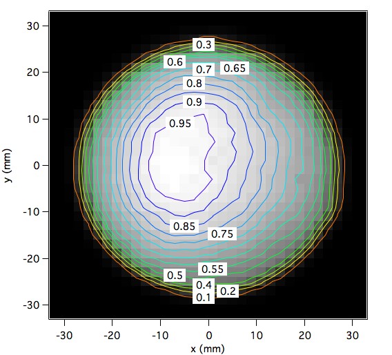
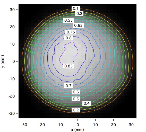
Estimates of the distribution of neutron density were used in the Monte-Carlo modeling of the experimental and systematic effects. The cold neutron beam from NG6 was mapped by activating a 25 m thick, natural-abundance dysprosium foil. Neutron absorption on 164Dy (28.2% abundance) follows the law, and the foil is thin enough to provide a sufficiently accurate measure of the neutron density. The activated foil was subsequently laid on a beta-sensitive film, and the exposure was measured with an image reader with pixel-resolution of 200 m by 200 m [42]. Maps 18 cm upstream and 18 cm downstream of the center of the detector array are shown in Fig. 4. The dominant features of the maps are the expansion of the beam (by about 5 mm in radius over the 80 cm length of the detector array) and the horizontal shift of the beam, which is due to the properties of the polarizer. The beam expansion affects the longitudinal cancelations of the from upstream-downstream combinations and leads to a systematic effect discussed in section VI.4.
IV.2 Polarization and spin flipper
The neutron polarizer is a supermirror bender (PSM) [44]. Neutrons are polarized parallel to the vertical magnetic field of the PSM. The spin flipper consists of two closely-spaced current sheets with horizontal currents. The magnetic field from the upstream current sheet was parallel to the PSM field, and the current in the downstream current sheet could be set parallel or antiparallel to the upstream current sheet. For antiparallel current, the vertical magnetic field reverses direction over a distance of about 1 mm corresponding to a time of about 2 s in the rest frame of a cold neutron. This time is short compared to the inverse Larmor frequency, and the neutron spin does not follow the magnetic field adiabatically. The result is that the neutron spin remains oriented in the original upward direction while the magnetic field reverses from up to down, thus reversing the projection of the spin with respect to the magnetic field direction. Small transverse neutron-spin components arise due to imperfect transitions. These transverse components precess around the magnetic guide-field as the neutrons move through the apparatus. Thus the polarization direction of a decaying neutron depends on the vertex of the decay as well as the neutron’s velocity and the magnetic field. The distribution of neutron velocities leads to azimuthal averaging of the transverse polarization components. The 560 T field was chosen so that the orientation of the neutron polarization varied by less than across the detector. Downstream of the spin flipper, the guide field adiabatically rotates the neutron spin into the longitudinal direction and remains longitudinal throughout the detector array.
The polarization was measured and mapped using a second polarizer as an analyzer downstream from the spin flipper [10]. A map of the estimated neutron polarization, assuming a perfect spin flipper and identical polarization and analyzing power (), is shown in Fig. 5. Though neither of these assumptions is accurate, this provides a lower limit on the neutron polarization [10]. The increase in polarization from left to right is a property of the polarizer and leads to effects that are discussed in section VI.5. When averaged across the beam, the lower limit on the neutron polarization is (90% c.l.), and we use in the analysis of . The polarization and spin-flipper characteristics appeared to be quite stable over long periods, and the measured polarization was consistent with that measured for the first emiT run, which set the lower limit of [9].

IV.3 Magnetic fields
Within the detector region, the magnetic field is maintained by a set of eight 0.95 m diameter coils uniformly spaced over 2 m. The outermost coils had independently adjustable currents, while the inner six coils were connected in series. The current, alignment, and position of each coil were set to optimize the longitudinal field uniformity. An array of longitudinal coils was deployed as a cosine magnet to cancel uniform transverse magnetic field components. These coils were also used to rotate the magnetic field for the transverse-polarization calibration runs. Additional trimming of non-uniform components of the magnetic field was necessary due to the magnetized steel in the floor and magnetic fields from other instruments in the NCNR guide hall [39, 40]. The currents in all coils were nominally constant with no active compensation; however, all currents were monitored, and the fields in the vicinity of the decay region were continuously measured using two 3-axis flux-gate magnetometers. Magnet-current and detector-field monitor data were used to define cuts on the data as described section VII.1.
The magnetic field in the detector region was mapped with a 3-axis fluxgate magnetometer before and after the emiT-II run. The large axial field of 560 T made precise measurement of transverse component difficult due to flexing of the support rail for the magnetometer; however, it was possible to estimate transverse components of 1-3 T. The corresponding magnetic-field misalignment was measured to be as large as 5.4 mrad, which was consistent with estimates based on the transverse-polarization calibration runs described in section VI.5.
IV.4 Detector overview
The detector array is shown schematically in Fig. 2. The main detector chamber was milled from a single block of aluminum. The chamber was supported on kinematic mounts and included mounts for cross-hair assemblies at both the upstream and downstream ends. Beam-line and detector components were mechanically positioned and aligned to better than 1 mm and 2 mrad, and the alignment was checked with crosshairs during final assembly.
The vacuum during data taking was maintained using a cryopump just downstream of the main detector chamber. In addition, liquid-nitrogen cooled cryopanels were situated at the ends of the proton detector assembly. The vacuum measured in this region was typically in the range of 3-4 Torr. This low pressure significantly reduced backgrounds due to neutron interactions with residual gas and minimizes the possibility of scattering and neutralization of decay protons. On the other hand, changes in proton detector dead-layer of roughly 3% per month, most likely due to the build-up of water and other volatile materials, were observed.
IV.5 Proton detectors
The proton-detector cell is illustrated in Fig. 3. Each cell consisted of a grounded box with the top and the upper half of the sides covered by a grounded wire mesh (97% transmitting) through which the recoil protons enter. Once inside the box, the protons were accelerated and focused onto the SBD (Ortec model AB-020-300-300-S) by the field produced by a cylindrical tube maintained at a negative potential with respect to ground. During the course of the experiment, the acceleration voltage was varied in the range kV to kV. Geometric constraints required that the SBD be positioned off-center relative to the focusing tube. In addition, the cryogenic epoxy holding the silicon wafer into its mount varied in thickness by up to one millimeter around the edge of the detector ring. These and other imperfections were included in the Monte-Carlo model of the proton focusing discussed in Section III. The proton SBD active layer was 300 m thick and 300 mm2 in area.
The proton detectors were periodically calibrated in situ with 241Am and 109Cd gamma-ray sources. Typical detector resolution was 4 keV FWHM but varied by several keV from channel to channel and over time. In most channels, thresholds were adjusted to reduce the count rates. This also resulted in truncating part of the accelerated proton spectrum introducing a proton-energy dependent efficiency and systematic effect discussed in section VI.3. Low energy tails on the proton peaks, observed in some channels, were of particular concern because of the thresholds. The source of these tails was inconclusive and may have been due to a combination of a number of possibilities including dead-layer buildup and scattering from the focusing tubes themselves. In addition, reversible build-up of the detector dead layers was observed to occur over time.
During the experiment detectors showed a variety of problems, including high leakage current and breakdown, and a portion of the data were taken with fewer than 64 operating SBDs. Over the course of the experiment, however, only a few SBDs were not operational at any one time, and when averaged over the entire run, every proton cell had a duty factor greater than about 90%.
IV.6 Electron detectors
Electron detectors are 50 cm by 8.4 cm by 0.64 cm thick BC408 plastic scintillators with Burle-8850 photomultiplier tubes (PMTs) at each end. The sensitive region of the electron detectors was fabricated from slabs of plastic scintillator cast to a thickness of 0.64 cm and diamond milled to a rectangular prism measuring 50 cm by 8.4 cm. The thickness was sufficient to stop a 1-MeV electron and was therefore adequate for detecting neutron decay electrons, which have an endpoint energy of 782 keV. The scintillators were wrapped in aluminized mylar and 20 m thick aluminum foil to prevent charging and to shield the detectors from x-rays and field-emission electrons. This thickness of aluminum stopped electrons of energy up to about 50 keV at normal incidence and led to energy loss of 20 keV for incident electrons with energy 200 keV. The foil and mylar were included in all Monte Carlo simulations.
Scintillation photons guided to either end of the scintillator by total internal reflection at the smooth surfaces were detected by the PMTs. An electron event requires coincidence of both PMTs within a timing window of 100 ns. The time difference of the phototube signals at the two ends of each scintillator was available to determine the electron position with resolution of about 10 cm but was not used in the analysis.
The electron detectors were calibrated periodically during the run using a 207Bi source. Conversion electrons from the source passed though a thin Kapton window into the vacuum chamber and were incident on the backside of the scintillator slabs passing through a hole in the mylar and aluminum foils. Gain drifts of up to 3% per month were observed, and PMT base voltages were occasionally adjusted to stabilize the gains. Remaining drifts were compensated run-by-run in the analysis using features of the neutron-decay-electron-energy spectrum. A threshold of 80 keV detected electron energy was applied to the data in order to eliminate the effects of residual gain drifts. The effects of remaining small nonuniformities in electron-energy threshold and response are discussed in Section VI.3.
IV.7 Monitors
The following parameters were continuously logged during data taking:
- 1.
Magnetic fields at two positions within the detector magnetic-field coils using 3-axis fluxgate magnetometers
- 2.
Currents in all magnetic field coils including neutron-guide solenoids and longitudinal and transverse detector coils
- 3.
The neutron capture-flux monitor
- 4.
Proton-cell acceleration voltage
- 5.
SBD bias voltage and current.
The cuts based on these monitor data were used to test for systematic effects and for cross checks of the results as discussed in section VII.1.
V Data
The neutron-decay data consist of proton-electron coincidence events that record which detectors were hit, amplitude of the pulse in each detector, spin-flipper state, and proton time-of-flight (). Data were acquired from October 2002 to November 2003 with some breaks for reactor and detector maintenance. The data were separated into runs of up to about four hours duration, and a total of 934 runs are included in the final data set.
Fig. 6 shows the detected proton energy versus proton time-of-flight for all events. Events prior to are random coincidences and are used to estimate background rates as described in section VI.1. The feature near primarily consists of true coincidences that are very closely spaced in time compared to neutron-decay-proton-electron events. These prompt coincidences arise from several sources including cosmic-ray muons and neutron capture , which produces gamma rays that produce a false proton-electron coincidence through Compton scattering or pair production. In Fig. 7 we show the proton-ADC spectrum for the timing window as a function of detected SBD amplitude. Protons, primarily from neutron decay are accelerated in the focusing cells and produce the narrow peak at 25 keV. The broad feature at higher energy is the minimum-ionizing peak for relativistic charged particles, e.g. from high-energy gamma interactions and cosmic rays. The pre-prompt data were used to estimate the random-coincidence contribution to the backgrounds discussed in section VI.1.

Typical count rates were 3 s-1 and 100 s-1 for single proton and electron detectors, respectively, while the coincidence rate for the entire array was typically 25 s-1. A total of raw events were acquired. Of these, limits on magnetic field, leakage current, and other monitors removed 12% of the events, the analysis threshold on electron energy removed 14% and the single electron hit requirement removed 7% of the raw events. The data were filtered by cuts on the parameters described in section IV.7 as well as on the detected electron-energy and the requirement of a single-electron-detector hit. We also rejected events during a spin flip and during an unpaired spin-flip cycles at the end of a run in order to ensure equal time in each spin-flipper state.
Most of the data were taken with nominal proton-acceleration voltages of 28 kV with smaller data sets at 25 kV, 27 kV, and 31 kV. The 27-kV data were acquired during the initial running stages in 2002. Discussion of the data and results for different proton-acceleration voltages, running conditions, and detector configurations are discussed in section VII.1.
| Description | Approximate number |
|---|---|
| Raw events | |
| Monitor cuts | (12%) |
| Electron-energy threshold | (14%) |
| Electron-detector multiplicity | (7%) |
| Final event sample | |
| Random coincidences |
VI Systematic Effects
Eq. 14 is based on an ideal symmetric experiment, which incorporates the following assumptions: a) accurate determination of the number of coincidences for each proton-cell-electron-detector combination, i.e. accurate background corrections; b) absence of proton and electron backscattering; c) symmetry of the detector, specifically the equivalence of proton cells and uniform proton and electron detection efficiencies; d) uniformity of the neutron beam; e) uniform longitudinal polarization; and f) accurate determination of and . A number of effects break the symmetries of the experiment and are accounted for by corrections to discussed in detail this section.
VI.1 Backgrounds
A valid event is defined as the coincidence of a proton-detector signal and electron-detector signal that meet the selection criteria on proton and electron energy, proton time-of-flight, and the monitor-data. Electron detection requires a coincidence of both phototubes in one scintillator panel with detected electron energy above 80 keV. The proton-energy-time-of-flight window is shown in Fig. 6. Background events that satisfy these criteria arise from several sources. Estimates of the background fractions for each component are discussed below, and the averages over all detectors, , are given in table 3.
Accidental Coincidences
The count rates for each spin-flipper state were corrected for accidental coincidences on a run-by-run basis by scaling the counts in the pre-prompt timing window () shown in Fig. 6. These random coincidences had the expected exponential dependence with respect to proton time-of-flight. A fit revealed a time constant of s, which is sufficiently long that we made no adjustment for proton time-of-flight. This results in a correction on the background subtraction estimated to be .
Prompt Coincidences
An energy spectrum of events in the prompt window (-0.75 s to 0.12 s) is shown in Fig. 7. The dominant components are the peak at 25 keV due to the accelerated protons from neutron decay, minimum ionizing charged particles predominantly due to cosmic-ray muons, and a background continuum. The low-energy behavior of the continuum was studied with high-voltage-off data, which eliminated the accelerated-proton peak. This component appears to fit well to a double exponential.
| Source | |
|---|---|
| Accidental coincidences | |
| Low-energy continuum | |
| Minimum Ionizing |
Background-related contributions to
The asymmetries must be corrected to determine the background-free asymmetries . The correction is
| (15) |
The first term is the multiplicative correction to due to the dilution of the asymmetries by backgrounds. This dilution can produce a contribution if the background corrections are non-uniform and do not completely cancel when the are combined into . The multiplicative correction to was determined using measured and according to Eq. 15 resulting in a correction to of . The multiplicative correction is dominated by the exponential components of the prompt events shown in Fig. 7. The second term in Eq. 15 is due to a possible asymmetry in the background, . The were found to be uniform and consistent with zero across the detector and were combined according to Eq. 14. The resulting was scaled by the sum of for all contributions to determine the additive correction to of . For the result reported in reference [11], no correction was made for the additive-background effect.
VI.2 Backscattering
Backscattering events fall into two categories: 1) particles scattered from somewhere in the apparatus to the proton or electron detector, and 2) incident protons and electrons that scatter from the respective detectors without registering a hit. Particles backscattered from the proton and electron detectors lead to multiplicative and additive corrections to the that can affect in a manner similar to background effects. Backscattering also affects and is discussed in section VI.6.
Backscattering corrections to were determined by Monte Carlo simulations with empirical validation based on studies of the and proton-electron coincidences. Backscattering probabilities are similar for all proton-electron-detector combinations; however, the rate of neutron-decay coincidence counts for the and pairings is about a factor of ten less than for the and pairings used to determine . Data from the and pairings are shown in the electron-energy-proton-time-of-flight plane in Fig. 8. The boxes indicate three distinct kinematic regions: primary neutron-decay events for the and proton-electron coincidences are restricted to a region included in region A; region B consists of higher energy electrons, which are primarily electrons with initial momentum directed at large angles with respect to the detected proton but detected in the or electron detector due to backscattering; region C corresponds to high energy electrons from events with large proton-electron angular separation and delayed proton time-of-flight, which are primarily due to proton backscattering. The backscatter fractions are estimated from the data by integrating within the boxes in Fig. 8 or by fitting the time-of-flight spectra and are consistent with the Monte Carlo predictions.
Electron backscattering

Electron backscattering was incorporated into the Monte Carlo simulations using penelope. The multiplicative correction to was determined using estimates of the backscattering fractions from the Monte Carlo to correct the measured similarly to the background corrections given in Eq. 15. With the correction applied, changes by , where the uncertainty reflects the 20% uncertainty assigned to the Monte-Carlo results due to limitations of the detector and beam model and limited knowledge of backscattering at these low energies. The additive correction would vanish for isotropic backscattering and uniform detector efficiency; however, the beam expansion, magnetic field, and detector elements break these symmetries. The result for the additive correction to is , and is limited by the statistical precision of the Monte Carlo due to the small fraction of backscatter events. This additive-electron-backscattering correction was not applied in the analysis reported in reference [11].
Proton backscattering
Backscattered protons in principle affect the asymmetries similarly to backscattered electrons. Proton backscattering probabilities determined with SRIM were input into the Monte Carlo. While the proton backscattering probabilities at the energies characteristic of neutron decay are comparable to electron backscattering probabilities, there is a large probability for neutralization [38]. Detailed calculations lead to the conclusion that proton-backscattering effects on are approximately an order of magnitude smaller than electron-backscattering effects, and we set an upper limit on the correction to of less than . This upper limit is reflected in the uncertainty given in Table 4.
VI.3 Efficiency corrections
The from Eq. 9 depend directly on the energy dependence of the efficiencies through the beta and neutrino correlations. Spatial variations of the proton and electron energy dependence break the symmetry assumed in combining proton-cell data as given in Eq. 14. In this section, we discuss the effects of axial and azimuthal variation of the electron energy thresholds and the variation of the proton-energy-dependent efficiency as a result of changes of individual SBD thresholds.
VI.3.1 Nonuniform electron-energy thresholds
From Eq. 12, it can be seen that the proton-electron correlation leads to a difference of for the two electron detectors that pair with (e.g and ). This leads to a contribution to from the beta-asymmetry (-coefficient correlation), which cancels for a uniform neutron beam and detector when the from two axially-symmetric proton cells are averaged (e.g. cells and ). In the case of nonuniform electron-detector efficiencies, specifically due to spatial variation of the electron-energy threshold, this cancellation is not perfect and leads to a dependence on the azimuthal proton-cell position, i.e. a dependence on proton-detector plane; however, another symmetry arises because each electron detector is paired with two azimuthally opposed proton cells and contributes to the two with opposite sign. This results in cancellation of any efficiency variation to first-order in , as given in Eq. 13. The dependence of , however, does not cancel.
The electron energy thresholds were measured to differ between upstream and downstream phototubes by as much as 10-20 keV resulting in the dependence evident in Fig. 9, where the combined data for for all proton cells in a single detector plane are shown as a function of . The dashed line shows the best fit to only, and the solid curve includes a contribution. Monte-Carlo studies with an upstream-downstream variation of electron threshold of approximately 10 keV for a single electron-detector show a similar contribution.
The Monte Carlo also shows that the axial dependence of the electron thresholds are cancelled when all four proton-detector planes are combined and therefore, does not contribute significantly to as long as the proton efficiencies are energy independent. The variation of proton energy dependent efficiency, discussed below, could couple with an electron-threshold variation. Coupling between the observed relative efficiencies of proton detection and the Monte-Carlo model of electron threshold variations had an effect on of .
VI.3.2 Proton-SBD efficiency variations (Shift-threshold effect)
A set of typical calibrated proton-cell SBD spectra is shown in Fig. 10 for both spin-flipper states and for both 125∘ and 145∘ coincidence angles. The electron detector at has approximately twice the rate as the detector due to the proton-electron correlation, which favors back-to-back proton and electron momenta. The spectra for the two spin-flipper states differ in both area (total number of counts, ) and the spectral distribution due to the beta asymmetry, which affects the angular distribution of electrons and thus the proton momentum. The energy deposited in the SBD in turn depends on the incident proton momentum, position and angle of incidence on the proton cell. We characterize each spectrum by a centroid, which depends on the neutron spin sate. The difference of the centroids for the two spin-flipper states varies with the axial position of each proton cell and varies in magnitude from zero to about 125 eV. In Fig. 11, we show the difference of the centroids as a function of proton-cell position for a single proton-detector plane (-) paired with the electron detectors at 125∘ and 145∘.
For the SBD spectra shown in Fig. 10, the low energy portion of the spectrum shows that the applied threshold allows detection of almost all of the protons for both electron detectors and both spin-flipper states. The SBD thresholds were adjusted throughout the run in order to maintain the electronics’ noise at a manageable level and minimize dead-time losses. In some cases, the threshold cut significantly into the SBD spectra introducing a proton-energy-dependent detection efficiency. Due to the dependence on neutron polarization, this energy dependence could lead to a significant effect on the for an SBD with a high threshold, though the effect on is largely mitigated because the low-energy portion of the proton energy spectrum is nearly equally affected for the two electron detectors. Fig. 12 shows that there are several notable anomalies of the , for example for proton cells and ; however, as expected, the anomalies are similar for both electron-detector pairings. Thus the , as shown in Fig. 13, do not appear to fluctuate significantly compared to other proton cells.


To estimate the effect on , neutron-polarization dependent proton energy spectra were generated by Monte Carlo for all proton-detector-electron-detector pairs and convoluted with model detector response. The model detector response (modified gaussians with separate widths above and below the centroid) were based on measured proton-SBD spectra. These spectra and the thresholds varied significantly during the course of the experiment, and the set of response functions was therefore based on an average over the data subsets. Parameters of the response functions were varied over a range characteristic of the variations during the experiment in order to estimate the uncertainties. The estimated correction to is . The effect was also estimated by correcting on a day-by-day basis using the centroid shift and slope at threshold with consistent results.
VI.4 Beam Expansion Correction
The neutron beam expansion affects the cancellation of the beta-asymmetry (Eq. 12) for axially-paired proton cells because the average of the electron velocity depends on the radial size of the beam: for decay vertices further from the center of the detector, the proton-electron angular separation is larger, which corresponds to higher energy electrons. This would be largely cancelled by the combination of the prescribed by Eq. 14 because the difference of enters with opposite sign for two adjacent proton cells ( and ); however, the magnetic field also affects the electron-proton angular correlation and therefore resulting in a magnetic-field dependence. The 560 T magnetic field makes the magnitude of the difference for the two electron detectors (e.g. and ) smaller for odd detectors (, , , etc.) than for even detectors (, , , etc.). The result is that the slopes of vs. have different magnitudes for even and odd proton cells. Fig. 14 shows a comparison of a uniform, nonexpanding neutron beam and the realistic beam based on the beam-distribution maps of Fig. 4. A possible systematic effect arising from the beam expansion coupling with a polarization gradient is discussed in section VI.5.
To estimate the correction, Monte Carlo simulations were run using the measured neutron-beam distribution. A number of simulations were run with different beam distributions produced by shifting the maps by up to 2 mm and rotating by 5∘, both significantly greater than the mechanical alignment constraints on the beam-line and detector components. In Fig. 15 we show the results for the beam expansion effect as a function of magnetic field. The estimated correction at T is is , where the uncertainty is mainly due to the change of the effect as the beam-distribution models were varied.

VI.5 Transverse polarization effects
As discussed in section II.2, transverse asymmetries arise in the experiment due to the polarization misalignment with respect to the detector axis. The misalignment was determined from the data combined with transverse-polarization calibration runs combined with Monte-Carlo simulation of the beam-shape effects and by magnetic field maps measured before and after the run. The transverse polarization leads to a contribution given in Eq. 13. For uniform-symmetric beam and polarization, and is cancelled when data from two opposing proton cells are combined; however, due to the asymmetric emiT-II beam, the cancellation is not complete. Displacement of the beam perpendicular to the transverse polarization would result in a contribution to that is the product of the polarization misalignment and the perpendicular misalignment of the beam. This is called the ATP or asymmetric-beam-transverse-polarization effect. An additional effect arises if the transverse polarization is nonuniform, specifically that varies along the axis of the detector.
VI.5.1 Asymmetric Beam/Transverse Polarization Effect
We have studied the ATP effect using transverse polarization calibration runs. Data from a transverse-polarization calibration run with is shown in Fig. 16. This amplifies the ATP effect, which is then scaled by the size of the transverse polarization for the run to determine the effect on . Calibration runs at several azimuthal angles map out the effect to provide a more accurate estimate. The size of the effect was also estimated in Monte Carlo simulations with and several different values of .
For calibration runs, the axial magnetic-field coils were used to cancel the Earth’s field component along the detector axis, and the transverse-field coils were used to produce a field of about 100 T perpendicular to the detector axis. The azimuthal angle could be selected; however, due to power supply limitations, the magnitude of the transverse field could not be maintained at 100 T for all azimuthal angles. In Fig. 16, we show the average for even and odd proton cells as a function of from a transverse polarization calibration run with and . A total of eleven polarization-calibration runs were taken over the course of the experiment. For each run, the amplitude and the offset are determined by fitting the data to a sinusoid. The average amplitude for all calibration runs with is
| (16) |
where the uncertainty is the standard deviation of the eleven amplitudes.

For the data runs, is small; thus the asymmetric beam shape contributes significantly to the dependence of the s. The beam maps shown in Fig. 4 show that, in addition to the beam expansion, the center of gravity of the beam is horizontally displaced from the detector axis and rises in the vertical direction for the downstream map. To separate the beam-shape and transverse-polarization effects, the were corrected for the beam-shape effect, which was determined from Monte Carlo simulations with no transverse polarization. The value of is found by dividing the amplitude of a sinusoid fit to the corrected by the average amplitude from the transverse-polarization calibration runs. In Fig. 17, we show results of Monte-Carlo studies for the beam-shape along with data and the resulting estimate of the transverse polarization effect. The Monte Carlo results for the beam-shape effect are very sensitive to the small differences in the beam-map registration and orientation. This results in large uncertainties in the transverse polarization direction. The results are
The uncertainty is determined from the uncertainty on and errors arising from the beam-shape correction and the effect (Fig. 9). Alternatively, using the magnetic-field maps discussed in section IV.3, we estimate
which is consistent with the analysis using the data and beam-shape correction. To determine the ATP correction, we use the 1- limits from the transverse-polarization calibration runs, which give
These limits provide more conservative bounds on the ATP effect than those base on the magnetic-field maps.
In Fig. 18, we show the data with fit and the result for the Monte-Carlo model of the experiment for . From the fit and the values of and given above, we determine the correction to of . The relatively large uncertainty is due to the uncertain azimuthal orientation of the polarization.


VI.5.2 Polarization twist
A twist of the polarization, that is an upstream-downstream difference in , would not be cancelled in combining 16 proton cell into . A limit on the polarization twist was estimated by separating data for upstream ( cm) and downstream ( cm) proton cells and correcting for beam-shape effects. The beam-shape corrected data are shown shown in Fig. 19. Sinusoid fits provide estimates for for upstream and downstream portions of the detector of and , from which we use to estimate a maximum upstream-downstream difference . We double to account for a change over the entire length of the proton-detector plane and use the fits from Fig. 18 to set an upper limit on the magnitude of the ATP-twist effect of of . This upper limit is reflected in the uncertainty listed in Table 4.

VI.5.3 Polarization nonuniformity
A nonuniform neutron polarization affects the cancellation of the electron () and antineutrino () asymmetries in . The polarization map, which measures the combination of neutron-beam polarization and the analyzer power , is shown in Fig. 5. Assuming , the polarization as a function of position was convolved with the density of neutron-decay vertices determined by Monte Carlo to determine an effective polarization for the decays detected by each proton cell. This was also studied using data from both transverse-polarization calibration runs and normal running. This effective polarization varied by a few percent along the beam axis due to the beam expansion; however, the average over all cells in each proton-detector varied by less than 0.005. The effect on was estimated by Monte-Carlo using the averaged polarization for each proton-detector plane. A possible transverse polarization gradient ( or ) was also investigated with the Monte Carlo and found to have a negligible effect.
VI.6 Uncertainties in Polarization and
Uncertainties in and lead to errors proportional to . The polarization analysis described in section IV.2 results in the lower limit (90% c.l.), and we take for the purpose of analysis. The resulting contribution to the uncertainty on is , which is given in Table 4. The kinematic quantities depend on the proton-electron angular separation due primarily to the cross-product , and are different for the and proton-electron-detector pairs. The were determined by Monte Carlo simulations, and a number of parameters were varied including beam size and shape, electron backscattering fraction, and electron-energy threshold. For proton-detector-electron-detector pairings at 125∘ and 145∘ we find and , where the uncertainties estimate the variation of as the Monte Carlo parameters are varied. The average, used to determine (see eq. 12) is
| (17) |
The resulting contribution to the uncertainty is .
VI.7 Spin flip and timing errors
Errors in the can also arise if the neutron polarization, flux, or counting time in each spin-flipper state is dependent on spin-flipper state. In these cases, the error is approximately proportional to . For example if the neutron flux or density within the detector is dependent on spin-flipper state, the count rates would be modified from the such that , where is the count rate for a spin-flip symmetric experiment and is the fractional change in the flux. In the event of a dependence of the flux on the spin-flipper state, the asymmetries would be modified from the spin-flip symmetric asymmetries . The measured asymmetry is
| (18) |
When the differences of the are combined into the and finally , the correction is
| (19) |
where we assume the measured is approximately equal to the corrected . A spin-flip correlated counting time difference () and polarization difference () introduce similar corrections.
Measured limits on the flux and counting time correlations with spin-flipper state are , and respectively. Thus the corrections to due to spin-flip correlated flux and counting time variations are less than . The spin-flipper efficiency was estimated to be greater than 0.95, implying and a correction to less than .
VI.8 Summary of Systematic Error Corrections
The corrections to are summarized in Table 4. The polarization and instrumental constant and are included in the definition of and are not included as corrections; however, the uncertainties on both are included in the table. The total correction is the sum of all corrections. The uncertainties are independent and are therefore combined in quadrature to determine the total systematic-error uncertainty.
a Polarization and are included in the definition of .
b Assumes polarization uncertainty of 0.05.
| Source | Correction | Uncertainty |
|---|---|---|
| Background additive | -0.07 | 0.07 |
| Multiplicative∗ | 0.03 | 0.09 |
| Electron backscattering additive | 0.09 | 0.07 |
| Multiplicative | 0.11 | 0.03 |
| Proton backscattering | 0 | 0.03 |
| Electron threshold non-uniformity | 0.04 | 0.10 |
| Proton-threshold effect | -0.29 | 0.41 |
| Beam expansion | -1.50 | 0.40 |
| Pol. non-uniformity | 0 | 0.10 |
| ATP - misalignment | -0.07 | 0.72 |
| ATP - Twist | 0 | 0.24 |
| Spin-correlated flux | 0 | |
| Spin-correlated polarization | 0 | |
| Polarization | a | 0.04b |
| a | 0.04 | |
| Total corrections | -1.66 | 0.97 |
∗ In reference [11] this entry had a typographical error.
VII Results
VII.1 Cross Checks
Several cross checks have been performed to validate the analysis and search for systematic errors. All cross checks were performed on blinded data. The cross checks fall into three main categories: 1) varying the cuts on experimental parameters, 2) breaking up the data into subsets, and 3) alternative definitions of that would be equivalent for an ideal experiment.
VII.1.1 Data Cuts
The original cuts on experimental parameters listed in section IV.7 were established using nominal operating parameters with windows set by typical variations that produced useful data (e.g. for the flux-gate magnetometer component: 5.56 G 5.62 G). To investigate the effects of the cuts, the nominal window was expanded by a factor of two in most cases (i.e. 5.53 G 5.65 G), and the change in was noted. For the electron-energy threshold the cut was lowered to 40 keV, which was below the threshold in some channels, and for electron-detector multiplicity, the cut was changed from one to two. With the exception of the proton acceleration voltage discussed below, changed by less than or 5% of the statistical error.
VII.1.2 Data-subset studies
Each independent measurement of combines from sixteen proton cells, all of which have relatively high efficiency for proton-electron coincidences; however, during the experiment, individual proton-cell SBDs were turned off for extended periods due to high leakage currents or noise. Possible variations of the results due to varying experimental conditions were studied by breaking up the experiment into subsets with roughly equal statistical weight. Subsets were separated by several possible changes including proton-acceleration voltage, number of live SBDs, and changes to the magnetic field prior to transverse-polarization calibration runs. For each of the four , 16 operating SBDs are required; however, a number of data subsets had one or more sets of proton-cells missing, in which case we report the weighted average of all available full sets of 16 proton-cells. The results for the subsets are shown in Fig. 20. A possible correlation of with high voltage was revealed in the study of cuts and investigated with data subsets shown in Fig. 20. Assuming is independent of acceleration voltage results in for 12 degrees of freedom. Allowing a linear dependence of with acceleration voltage results in for 11 degrees of freedom. The change in implies a 2.1-sigma slope. In addition, the acceleration-voltage dependence of the focusing properties was extensively studied by Monte Carlo simulations, which showed no effect correlating with acceleration voltage. We therefore consider the preference for a slope to be an accidental correlation.
VII.1.3 Alternative definitions of
The definition of given in Eq. 14 averaged the smallest number of proton cells (i.e. 16), which cancelled the beta and neutrino asymmetries in the presence of transverse polarization and the 560 T magnetic field. Our final result, the weighted average of the four independent determinations of , thus has the smallest possible statistical error. For a uniform detector and beam, can also be defined as a) the simple average of all 64 , which differs from only due to small changes in weighting of the individual ; b) the average of the combined data from four individual proton-detector planes; c) the offset when the are fit to a sinusoid (Eq. 13); d) the offset for the sinusoid fit when the averages of for each proton-detector plane; or e) the paired proton-cell approach used in the analysis of emiT-I data [9]. The results for are all found to be consistent with for all analyses based on , i.e. a)-d). The paired-proton-cell approach, method e), is known to be very sensitive to the proton-threshold effect discussed in section VI.3 and produced a significantly different value. Correcting for the estimated proton-threshold effect on based on day-to-day correction of the yielded a value consistent with . Cross checks were also performed on data subsets and found to be consistent with the exception of the 31-kV data for which a large number of proton cells were dead.
A blind analysis of the asymmetries was adopted by adding a quantity to each (equation 9) so that when was extracted from Eq. 14 it was offset from the true value by , where . The factor was revealed and subtracted as the final analysis step, after the corrections for systematic errors and all uncertainties were determined.
VII.2 Final Result
When averaged over the entire run, each SBD was live for a majority of the time and had a high average efficiency. We can therefore combine counts for the entire run to determine the s and to extract for each set of 16 proton cells. The results for the four separate are presented in Fig. 21 and Table 5. The weighted average of the four is . When combined with the total of corrections listed in Table 4, our final result is
| (20) |
This differs from reference [11] due to refinement of the additive corrections due to background and backscattering, which changed by and , respectively.

| Proton-cell set | (cm) | |
| 1 | 2 | |
| 2 | 6 | |
| 3 | 10 | |
| 4 | 14 | |
| Average |
VIII Conclusions
Our result represents the most sensitive measurement of in nuclear beta decay and can be interpreted in terms of possible extensions of the Standard Model. Rewriting Eq. 7:
where and , and we have neglected the order- radiative corrections, which yield negligible contributions given the existing limits on scalar and tensor currents.
Assuming no scalar or tensor currents, our result constrains the complex phase between the axial-vector and vector currents ( ) to (68% confidence level). If all currents are allowed, for example due tor leptoquark exchange, the equation contains five phases, making it difficult to compare the sensitivity of our experiment with respect to other probes without further assumptions. In the specific case where there are no special cancellations between terms, we estimate the sensitivity of our measurement under two different assumptions. Fig. 22, left panel, shows the limits on the imaginary component of the scalar currents, assuming that the tensor currents are purely real and equal to the largest value allowed by present constraints. In this case, because the limits on are much smaller than those on our result is most sensitive to the imaginary component of . The right panel shows a similar plot but now assuming that scalar currents are purely real and equal to the largest value allowed by present constraints.
VIII.1 Potential Improvements
The result for presented here has comparable statistical and systematic uncertainties. Thus an improved experiment with the same apparatus would need both more neutron decays and reduced systematic effects. A new beam-line (NGC) under construction at NCNR and the PF-1 beam at ILL could provide a factor of 10 or more decays per unit time. Reducing the three major systematic corrections requires eliminating the proton-threshold variations, a more symmetric neutron beam, and smaller magnetic field. The symmetry of the neutron-beam is most strongly affected by the supermirror-bender neutron polarizer, while the 560 T magnetic field was chosen to effect sufficient velocity averaging of transverse-neutron polarization produced in the current-sheet spin flipper. An alternative polarizer is a steady-state polarized 3He spin filter [49]. Intense cold neutron beams have been shown to affect the rubidium and 3He polarization [50]; however, this appears to be a solvable technical challenge [51]. The 560 T guide field can be reduced by using an adiabatic-fast-passage neutron spin flipper and effective shimming of the magnetic field along with shielding of external field perturbations. Thus a factor of three or more improvement in sensitivity to appears within reach with the current apparatus. Extending the sensitivity to the level of final-state-effects () and beyond is a well motivated goal that would require an apparatus with greater geometric efficiency for both proton and electron detectors.
Acknowledgements
The authors gratefully acknowledge informative conversations with Wick Haxton, Michael Ramsey-Musolf, and Sean Tulin. The emiT apparatus and emiT-I experiment were developed by many additional collaborators including Shenq-Rong Hwang, Laura Lising, Hamish Robertson, and Tom Steiger along with Bill Teasdale. The neutron facilities used in this work were provided by the National Institute of Standards and Technology, U.S. Department of Commerce. The research was made possible in part by grants from the U.S. Department of Energy Office of Nuclear Physics (DE-FG02-97ER41020, DE-AC02-05CH11231, and DE-FG02-97ER41041), and the National Science Foundation (PHY-0555432, PHY-0855694, PHY- 0555474, and PHY-0855310).
- [1] D. Dubbers, M.G. Schmidt, Rev. Mod. Phys. 83, 1111Ð1171 (2011).
- [2] C.A. Baker et al. Phys. Rev. Lett. 97, 131801 (2006).
- [3] W.C. Griffith et al. Phys. Rev. Lett. 102, 101601 (2009).
- [4] M.A. Rosenberry and T.E. Chupp Phys. Rev. Lett. 86, 22 (2001).
- [5] V. M. Abazov et al. (D0 Collaboration) Phys. Rev. Lett. 105, 081801 (2010).
- [6] A. Riotto and M. Trodden, Ann. Rev. Nucl. Part. Sci. 49, 35 (1999).
- [7] S. Davidson, E. Nardi, and Y. Nir, Phys. Rept. 466, 105 (2008).
- [8] T.J. Bowles, NBS SP 171, 69 (1986).
- [9] L.J. Lising et al. Phys. Rev. C, 62, 055501 (2000).
- [10] H.P. Mumm et al., Rev. Sci. Inst, 75, 5343 (2004).
- [11] H. P. Mumm, T.E. Chupp, K.P. Coulter, R.L. Cooper, S.J. Freedman, B.K. Fujikawa G.L. Jones, A. Garcia, J.S. Nico, A.K. Thompson, C. Trull, F.E. Wietfeldt, J.F. Wilkerson, Phys. Rev. Lett. 107, 102301 (2011).
- [12] J.D. Jackson, S.B. Treiman, and H.W. Wyld Jr., Phys. Rev. 106, 517 (1957).
- [13] J.C. Hardy and I.S. Towner, Phys. Rev. C 79, 055502 (2009).
- [14] B.R. Holstein Phys. Rev. C 28, 342 (1983); B. Holstein, Weak Interactions in Nuclei, 166 Princeton (1989).
- [15] J.D. Jackson, S.B. Treiman, and H.W. Wyld Jr., Nucl. Phys. 4, 206 (1957).
- [16] C.G. Callan and S.B. Treiman, Phys. Rev. 162, 1494 (1967).
- [17] S. Ando, J. McGovern, T. Sato, Physics Letters B 677, 109 (2009).
- [18] I.B. Khriplovich, Nucl. Phys. B 352, 385 (1991).
- [19] R.S. Conti and I.B. Khriplovich, Phys. Rev. Lett. 65, 3262 (1992).
- [20] W.C. Haxton, A. Höring, M.J. Musolf, Phys. Rev. D 50, 3422 (1994).
- [21] A. Kurylov, G.C. McLaughlin, M.J. Ramsey-Musolf, Phys. Rev. D 63, 076007 (2001).
- [22] J. Ng and S. Tulin, Phys. Rev. D 85, 033001 (2012).
- [23] T. Soldner et al., Phys. Lett. B 581, 49 (2004).
- [24] K. Nakamura et al. (Particle Data Group), Jour. Phys. G 37, 075021 (2010).
- [25] R. I. Steinberg, P. Liaud, B. Vignon, and V. W. Hughes, Phys. Rev. Lett. 33 41 (1974).
- [26] B.G. Erozolimsky et al., JETP Lett 20 345 (1974).
- [27] B.G. Erozolimsky et al., Yad Fiz. 28 98 (1978).
- [28] P. Herczeg. and I.B. Khriplovich, Phys. Rev. D 56, 80 (1997).
- [29] P. Herczeg, in Proc. of the 6th Int. PASCOS-98, edited by P. Nath (World Scientific, Singapore, 1998).
- [30] A.L. Hallin, F.P Calaprice, D.W. MacArthur, L.E. Pillonen, M.B. Schneider, D. F. Schreiber, Phys. Rev. Lett. 52, 337 (1984).
- [31] F. Calaprice, in Hyperfine Interactions (Springer, Nether- lands), Vol. 22. (1985).
- [32] A. Kozela et al., Phys. Rev. Lett. 102, 172301 (2009).
- [33] J. Sromicki, M. Allet, K. Bodek, W. Hajdas, J. Lang, R. Müller, S. Navert, O. Naviliat-Cuncic, J. Zejma, and W. Haeberli, Phys. Rev. C 53, 932 (1996).
- [34] J. Sempau et al., Nucl. Instr. Meth. in Physics Research B 132, 377 (1997). Distributed by OECD Nuclear Energy Agency Data Bank.
- [35] J. Martin et al. Phys. Rev. C 68, 055503 (2003), Phys. Rev. C 73, 015501 (2006).
- [36] Ion Source Sofware, simion 3D Ion Optics Programs, http://http://simion.com/. Certain trade names and company products are mentioned in the text or identified in an illustration in order to adequately specify the experimental procedure and equipment used. In no case does such identification imply recommendation or endorsement by the National Institute of Standards and Technology, nor does it imply that the products are necessarily the best available for the purpose.
- [37] J. F. Ziegler, J. P. Biersack and M. D. Ziegler, The Stopping and Range of Ions in Matter, SRIM Co. (2008); http://www.SRIM.org.
- [38] S.K. Allison, Rev. Mod. Phys. 30, 1137 (1958).
- [39] S.R. Hwang, PhD. Dissertation, University of Michigan, pp 21-42 (1998).
- [40] H.P. Mumm, PhD. Dissertation, University of Washington, pp 39-44 (2003).
- [41] L.J. Lising, PhD. Dissertation, University of California, Berkeley, (1999).
- [42] Y. T. Cheng, T. Soodprasert and J. M. R. Hutchinson. Appl. Radiat. Isot. 47, 1023 (1996).
- [43] Manufactrured by LND, Inc., Oceanside, New York, 11572, USA.
- [44] O. Schaerpf, Physica B 156-157, 631 (1989)
- [45] E.G. Adelberger et al., Phys. Rev. Lett. 83, 1299 (1999).
- [46] A. Gorelov et al., Phys. Rev. Lett. 94, 142501 (2005).
- [47] C. H. Johnson, Fr. Pleasonton, T. A. Carlson Phys. Rev 132, 1149 (1963).
- [48] R. Huber et al., Phys. Rev. Lett. 90, 202301 (2003).
- [49] T. Chupp et al., Nucl. Inst. and Meth in Physics Res. A 574, 500 (2007).
- [50] M. Sharma et al., Phys. Rev. Lett. 101, 083002 (2008).
- [51] E. Babcock et al., Physica B 404 2655, (2009).