Quasi-classical approximation in vortex filament dynamics. Integrable systems, gradient catastrophe and flutter
Abstract
Quasiclassical approximation in the intrinsic description of the vortex filament dynamics is discussed. Within this approximation the governing equations are given by elliptic system of quasi-linear PDEs of the first order. Dispersionless Da Rios system and dispersionless Hirota equation are among them. They describe motion of vortex filament with slow varying curvature and torsion without or with axial flow. Gradient catastrophe for governing equations is studied. It is shown that geometrically this catastrophe manifests as a fast oscillation of a filament curve around the rectifying plane which resembles the flutter of airfoils. Analytically it is the elliptic umbilic singularity in the terminology of the catastrophe theory. It is demonstrated that its double scaling regularization is governed by the Painlevé I equation.
1 Introduction
Dynamics of vortices has been the subject of intensive study since the pioneering works of Helmholtz, Lord Kelvin and Poincaré in the 19th century (see e.g. [1, 2]). Relatively simple dynamics of a thin vortex filament in an incompressible inviscid fluid and in an infinite three-dimensional domain has attracted a particular interest.
An approach based on the localized induction approximation (LIA) has been proposed in 1906 by Da Rios [3]. Within such approximation one assumes that the vorticity is confined to a thin vortex core region and the core radius of the vortex tube is much smaller than the radius of curvature at the point and, hence, the induced velocity at this point is dominated by the contribution from the neighboring segment. Using the Biot-Savart formula
| (1) |
under the assumption that the circulation of the vortex is a constant, one gets
| (2) |
where denotes a point on the filament, is the arclenght, is time, is curvature, denotes the binormal vector and is the length of the segment of the filament whose contribution into the induced velocity is taken into account in the integral (1). Assuming that one can neglect the variation of along the filament, rescaling time by the constant and using the expression of in terms of , one obtains
| (3) |
Thus, within LIA approach, one has a simple binormal motion of the filament with the induced velocity proportional to the curvature . Using the Serret-Frenet formulae for the space curves, one can transform (3) into the system of intrinsic equations for the curvature and torsion which is of the form [3]
| (4) |
These LIA and Da Rios system have been rediscovered sixty years later in [4, 5, 6]. The detailed historical account of this story is presented in [7].
An important step in the development of the LIA approach has been done by Hasimoto in 1972 [8]. He observed that the system (4) is equivalent to the focusing nonlinear Schroedinger equation (NLS)
| (5) |
via the transformation
| (6) |
The NLS equation was already widely known in plasma physics. Moreover in 1971 Zakharov and Shabat [9] discovered that NLS equation (5) is integrable by the inverse scattering transform (IST) method. Hasimoto’s result has demonstrated that the whole powerful machinery of the IST method (solitons, infinite sets of integrals of motion, symmetries etc.) is applicable to the vortex filament dynamics. This fact has lead to the explosion of interest to this field and since that time various aspects of the LIA in the vortex filament dynamics have been studied by different methods (see e.g. [10]-[36]). Instabilities of vortex filament and formation of singularities were two important problems partially addressed during this period [16, 28, 35].
At the same time it was clear that LIA is too restrictive since it neglects several important effects like axial flow, stretching, shortening, filament core structure etc. Attempts to go beyond LIA have been done in [37]-[42]. In particular, the inclusion of the axial flow into consideration has lead to the following expression for the induced velocity
| (7) |
where is the tangent vector, are some parameters defined by the called matching condition, is a certain vector and denotes the contribution from the nonlocal effects. In situation when one can neglect and variation of along the filament, the vector can be chosen as . After a rescaling of time equation (7) takes the form [41]
| (8) |
where is the normal vector, is a certain parameter related to the intensity of the axial flow. After the Hasimoto transformation (6) equation (8) becomes
| (9) |
that is the Hirota equation or the linear combination of the NLS and first higher NLS equation [43]. It is again an integrable equation. On the other hand it describes new effects such as axial flow, local stretching proportional to , binormal velocity depending on torsion , effects which were not caught by LIA equation (3). It was shown in [41] that axial flow affects essentially stability properties of the filament.The observation that the simple generalizations of equation (3) or Da Rios system (4) may describe important nonlinear effects essential for vortex filament dynamics was one of the main results of [41]. Another observation made in [41] based on the paper [6] is that the study of the quasiclassical (or dispersionless) limit of the equation (9) clarifies essentially an analysis of destabilizing effects in the vortex filament motion.
The latter result was strongly supported by the recent study of the modulation instability of the focusing NLS and higher NLS equations (see e.g. [44]-[58]). In these papers it was shown that the dispersionless limit of the NLS equation (dNLS) is quite relevant to the study of the modulation instability. In this limit NLS is the elliptic system of quasilinear PDEs which exhibits the gradient catastrophe behavior at finite time. Behavior of solutions near to the points of catastrophe and beyond has been studied in details in [52]-[58]. It was argued in these papers that the gradient catastrophe for dNLS is a source of the modulation instability for NLS.
The above two facts clearly indicate the importance of the integrable systems modeling certain effects of vortex filament dynamics and of their quasiclassical (or dispersionless) limit.
Moreover, the results of the papers [39, 40], showing that the cutoff is not a constant but strongly depends on curvature and torsion of filament, manifestly show the necessity to go beyond the approximation described by equations (8) and (9). Indeed, in general case, the parameters in (7) are some functions of , the vectors and are certain superpositions of , , and and then the induced velocity is of the form
| (10) |
where A,B,C are some functions. Equation (10) implies certain intrinsic equations for and which, for particular choices of A,B,C, are integrable systems [17] different from (9). Relevance of these equations for the vortex filament dynamics is definitely of interest.
Study of the quasiclassical approximation for the intrinsic equations associated with the motion (10) and their implications for the vortex filament dynamics is the main goal of the present paper. Quasiclassical intrinsic systems describe motions of vortex filament with curvature and torsion slowly varying along the filament and in the motion, i.e. they are systems of equations for , where and are slow variables defined as , , (see e.g. [59]). For the Da Rios system (4) one has
| (11) |
or, in terms of Riemann invariants
| (12) |
For the intrinsic system associated with equation (9) (see [41]) and others the corresponding quasiclassical equations are of the form
| (13) |
where the characteristic velocity is an appropriate function of and .
In this paper we will concentrate on the study of the equation
| (14) |
which is the the quasiclassical limit of the intrinsic equations corresponding to the evolution of the filament of the type (10) with
| (15) |
where and being real constants. First two terms in r.h.s. of (14) represents themselves the quasiclassical limit of equation (9) (see equations (3.76),(3.77)) from ([41] with ), while the last term is of different type. Thought the corresponding contribution to the velocity (10) is quite complicated (15) the equation describing this flow separately is a very simple one. It is equivalent to the equation
| (16) |
which is the dispersionless Toda (dToda) or the Boyer-Finley equation [60]-[63]. dToda equation is integrable and plays an important role in various physical phenomena (see e.g. [63]-[67]). It is known also that dToda and dNLS equations belong to the same dToda/dNLS hierarchy (see e.g. [52, 67]). While the first two terms in r.h.s. of (14) represent “positive” members the last (dToda) term is the first “log-type” term. The presence of such dToda contribution into the induced velocity (10), even if not completely justified in a model independent way, could be of phenomenological importance since it might describe nonlinear effects different from those captured by equation (9).
Ellipticity of equation (14) or, in general, of (13) suggests to write it, following to [68, 69, 70], as the nonlinear Beltrami equation
| (17) |
So, a solution of equation (14) defines (see e.g. [68, 69, 70]) quasiconformal mapping if
| (18) |
In particular, any solution of the dDR system (11) defines a quasiconformal mapping on the plane . Quasiconformal mappings definitely play an important role in the vortex filament dynamics.
According to the result of papers [50]-[58], equation (14) well approximates the corresponding full equation of motion (equation at ) until the derivatives and are not large. Analysis of behavior of solutions of equation (14) near the point of gradient catastrophe, where and become unbounded, is the main subject of our study. Some results concerning dDR equation (equation 14 with ) have been reported briefly in [71]. Here, following the same approach, we will analyze the full equation (14). We will see that the inclusion of these two terms essentially modify the behavior of vortex filament.
Our approach starts with the observation that the hodograph solutions of equation (14) describe critical points of the function which obeys the Euler-Poisson-Darboux equation , i.e.
| (19) |
This fact essentially simplifies the analysis of the singular sector for equation (14) associated with the gradient catastrophe.
Since the points of gradient catastrophe belong to a singular sector in the space of solutions of the system (14) for which . Generic points of are characterized by the condition while for deeper singular subsectors , all the derivatives of vanish up to . For these subsectors one has constraints on all variables parameterizing . In particular, generic gradient catastrophe happens in a single point .
Vortex filament exhibits a very particular behavior at the point of gradient catastrophe. While at a regular point (with bounded , ,, ) a curve modeling the filament always lies of one side of the rectifying plane (spanned by the tangent vector and the binormal vector ), at the point of gradient catastrophe it oscillates fast around the rectifying plane. In addition, center of the osculating sphere (and its radius) blows up to infinity. Moreover, the induced velocity becomes unbounded at the point , . So, the gradient catastrophe for the system (14) give rises to the fast oscillations which resemble the classical airfoil flutter (see e.g. [72]). Numerical results [48] show that such oscillations begin to expand along the filament [71]. Such a behavior of filament clearly indicates on its instability.
Analytically at the point of gradient catastrophe one has a catastrophe of certain type. Using the double scaling limit technique we show that at the generic point of gradient catastrophe (i.e. in the sector ) one has the elliptic umbilic catastrophe in terminology of R. Thom [73] with the principal part given by . Deeper gradient catastrophes are associated with higher singularities. For example, in the sector the corresponding singularity is given by singularity from the V. Arnold list [74] with the principal part of the form .
At the point of gradient catastrophe the quasiclassical approximation becomes invalid and the system (14) should be substituted by its full dispersive version (by the intrinsic version of equation (8) at ). First order corrections can be obtained by the double scaling technique together with an appropriate modification of the function to a functional such that the equation for critical points are substituted by the Euler-Lagrange equation for . It is shown that for generic point of gradient catastrophe (i.e. the sector ) the resulting equation for small corrections is equivalent to the Painlevé I equation
| (20) |
The result of the paper [52] allows us to conjecture that any generic solution of the Da Rios system (4) at the point of gradient catastrophe behaves as and where is described by the tritronqueé solution of the Painlevé I equation.
It is shown also that a class of double scaling regularizations of the higher gradient catastrophes associated with sectors is described by the equations
| (21) |
The paper is organized as follows. In section 2 the relation of hodograph solutions with Euler-Poisson-Darboux equation is discussed. In section 3 it is shown that the hodograph solutions of dToda/dNLS equation describe critical points of a function. Hydrodynamic analogy and quasiconformal mappings for the governing equations are considered in section 4. Next section is devoted to an analysis of gradient catastrophe. Geometrical implications of gradient catastrophe and flutter of vortex filament are described in section 6. In section 7 it is shown that in the point of gradient catastrophe one has elliptic umbilic, and other singularities. Double scaling regularization of these catastrophes is analyzed in section 8.
2 Hodograph solutions and Euler-Poisson-Darboux equation
The dDR system (12), equation (14) and general two-component elliptic quasilinear system written in terms of Riemann invariants, i.e. (13) are linearizable by the classical hodograph transformation (see e.g. [75, 76]). One has
| (22) |
For equation (13) in the form of nonlinear Beltrami equation (17) the corresponding linearized equation is
| (23) |
The compatibility condition for the system (22) is given by the second order equation
| (24) |
solutions of which provide us with solutions of hodograph equations (22). In the hyperbolic case, i.e. for hydrodynamic type equations, equation of the type (24) has been widely used for the construction of the solutions and an analysis of their properties (see e.g. [75, 76, 77]).
In our elliptic case, equation of type (24) written in term of variables , and defined as , i.e. the equation
| (25) |
has been applied to the study of the system
| (26) |
which appears in the theory of wave processes in unstable media within nonlinear geometric optics approximation [78, 79]. At it is the quasiclassical limit of the focusing NLS equation (5) or the dDR system (11) for , . In particular, in the paper [80], the behavior of the solutions for the system (26) near the singular point of equation (25) has been studied. For the hyperbolic version see also [81]
For the dDR system (12) equation (24) is particularly simple one
| (27) |
It is the Euler-Poisson-Darboux (EPD) equation of type (see e.g. [82]). For the dToda equation , equation (24) is of the form
| (28) |
that is again the simple EPD equation of the type .
In contrast, for equation (22) with which corresponds to the second term in (14) and to the quasiclassical limit of the first higher NLS equation (see formula (9)), equation (24) is
| (29) |
For higher dNLS equations this equation is more and more complicated and hence an analysis similar to that performed in [79, 81] becomes much more involved.
A way to simplify drastically equations of type (24) associated with equation (24) can be extracted from the Tsarev’s [83] discussion of the generalized hodograph equations. He noted that it is convenient to rewrite equation (22) as
| (30) |
Denoting , one observes that and equation (30) assumes the form
| (31) |
So, equation (30) and, hence, the hodograph equation (22) takes the form
| (32) |
where is any function obeying the constraint (31). In the form (32) the hodograph equations can be formulated also for multi-component hydrodynamic type systems [83].
An observation here is that for the dDR system (11) and equation (12) one has
| (33) |
and, hence,
| (34) |
Furthermore, these equations imply that
| (35) |
where and are certain real valued functions. For instance, for equation (14)
| (36) |
In virtue of (33) and (34) the functions and obey the EPD equation
| (37) |
So, the hodograph equation (30) is of the form
| (38) |
where and are solutions of the same EPD equation . It remains to note that
| (39) |
is a solution of the equation (24) with .
Thus, in contrast to the usual approach in which hodograph solutions of the commuting quasilinear systems contributing into the r.h.s. of equation (14) can be found via different linear second order equations (see equations (19),(28), (29)), in the approach described above all of them can be build via solutions of the same and simple EPD equation .
3 Quasiclassical intrinsic equations for dToda/dNLS hierarchy and critical points of functions
In addition to the observations made in the previous section, one readily concludes that the hodograph equation (38) can be represented as
| (40) |
where
| (41) |
and the function obeys the EPD equation
| (42) |
Thus, one has
Proposition 3.1.
In the hyperbolic case, i.e. for the quasiclassical shallow water equation (or one-layer Benney system) this fact has been observed in [88] (see also [89]).
So, in order to construct a solution of equation (14) one takes a function of the form (41) with function given by (36), arbitrary functions solving EPD equation and finds its critical points solving equation (40). The class of solutions obtained in this way is controlled by the class of solutions of the EPD equation. Various classes of solutions of this equation has been described a century ago (see e.g. [82]) as well as in recent papers concerning the application of the EPD equation in Whitham theory. For example, a class of solutions of the EPD equation is given by
| (43) |
where is the positively oriented circle of large radius and is an arbitrary polynomial of the complex variable parameterized by the constants (see e.g. [88, 89]). In particular, the function (41) with is given by (43) with and . Parameters in and can be viewed as the variables parameterizing a class of initial data for equation (14).
In terms of curvature and torsion the EPD equation (42) is of the form
| (44) |
that is the axisymmetric three dimensional Laplace equation studied by Beltrami [90] (see also [75]). Here and play the role of the radial and axial coordinates, respectively, in the cylindrical system of coordinates.
Function (41) is
| (45) |
and hodograph equations are given by
| (46) |
The corresponding system of quasilinear PDEs in terms of and is of the form
| (47) |
At it coincides with the dispersionless limit of the equations given in [41]. We note that the contribution from dToda terms (with ) are quite different from those of dispersionless Hirota equation ((47) with ) considered in [41]. Formally at small , the last terms in (47) becomes dominant. Essential difference between the dDR and dHirota type evolution and dToda contribution is manifested by the expression (15) of the velocity of filament. The former are small for filaments close to a straight line (small ) and becomes larger for more curved filaments. In contrast, the dToda type contribution to the induced velocity (proportional to ) is smaller for larger and increase with decreasing . Since in the approximation under consideration always the dToda type contribution might be relevant for the description of some nonlinear and nonlocal effects appearing for slightly curved vortex filaments.
In virtue of (42) at the critical points of the function given by (40) or (46) one has
| (48) |
or
| (49) |
The point is a singular point for these equations. Analysis of the behaviors of solutions of these equations near this point can be performed in a way similar to that discussed in [80].
Geometrically the case corresponds to a straight line. In this paper we will be interested in properties of curved vortex filament. In the rest of the paper we will assume that . So, equations (48) and (49) take the form
| (50) |
and
| (51) |
We will see that these conditions simplify essentially an analysis of singular sector for equation (14).
4 Ellipticity of governing equations: hydrodynamic analogy and quasiconformal mappings
Ellipticity of the dDR system (11) and more general system (47) means that they have properties drastically different from those of the hyperbolic version of the dDR system (or the system (26) with ), that is the classical shallow water equation (see e.g. [76]). The latter has standard Riemann wave solutions while in the elliptic case the Cauchy problem is ill posed. In spite of such a difference a representation of the elliptic systems in the form of hydrodynamic type systems, but with negative pressure, has been widely used in the analysis of their local properties (see [6, 78, 79, 41, 45]).
Following this line one can rewrite the system (47) in terms of and as
| (52) |
where
| (53) |
Here , , and play the roles of density, velocity and pressure. Note that the system considered in [41] is not a system of quasi-linear equations. It contains the terms nonlinear in first order derivatives in addition to those quasi-linear ones in the system (47) with . Moreover our definition of the velocity and pressure is slightly different from those from [41]. Consequently, the system (52) is composed exactly by the continuity and Euler equations in contrast to the system (3.79)-(3.80) from [41].
Properties of the system (52) are fully determined by the properties of the pressure (53). Within LIA the pressure is always negative and that causes the well-known instability of vortex filament. Inclusion of the Hirota and dToda contributions changes the situation drastically. For large curvature axial flow contributions dominate and the sign of the pressure is different for different values of and . For instance, if then the pressure P for large and is positive, while in the opposite case it is negative. Then, for the points with small (near flattening points) one has stabilizing effect () while, with large torsion dHirota contribution (i.e. axial flow contribution) always destabilize the filament (recall that ).
For small (small density) pure dToda contribution equal to dominates the pressure. So, for small the sign of the pressure coincides with the sign of . Hence, once again one has a threshold dividing the regimes with positive and negative pressure and consequently stabilizing and destabilizing effects of contributions different from the original LIA model of Da Rios. If one considers the contribution only from axial flow () the pressure is
| (54) |
vanishes for and connected by the relation , while it is positive for vortex filaments with curvature and torsion obeying the condition
| (55) |
and it is negative in the opposite case.
This discussion shows that stability or instability of vortex filaments strongly depends on their geometry (relations between curvature and torsion).
There is another way to formulate and emphasize an ellipticity of governing equations. The dDR system (12) and more generally system (13) are elliptic systems of quasilinear equations and, hence, under certain conditions their solutions define quasiconformal mappings on the plane (see e.g. [68, 69, 70]). Introducing the independent variable , one can rewrite general equation (22) in the form
| (56) |
It is the nonlinear Beltrami equation [68, 69, 70] solution of which defines a quasiconformal mapping iff the dilation coefficient obeys the constraint . This condition, i.e.
| (57) |
imposes constraints on and, hence, on and . For the dDR system (11), , and one has
| (58) |
Since one always has for any nonstraight filament.
So, the slow motions of nonstraight vortex filaments within original LIA are described by quasiconformal mappings on the plane defined by the equation
| (59) |
For the generalization of the LIA given by equation (9) or (14) situation is more complicated. For equation (14) with one has
| (60) |
and the condition is verified if and and parameter obey the constraint
| (61) |
So, only part of the vortex filament configurations with axial flow is associated with the quasiconformal mappings, a sufficient condition being . For the complete flow (14) the constraint on and is more complicated. It is of interest to note that for pure dToda equation
| (62) |
corresponding to the last term in (14), one has
| (63) |
So, solutions of the dToda equation define a quasiconformal mapping iff . At equation (62) is equivalent to the equation
| (64) |
and and, hence, any solution of the dToda equation (64) defines a quasiconformal mapping on the plane.
The results of the previous sections indicate also a relation between certain class of quasiconformal mappings on the plane and EPD equation. Indeed, solutions of equation (40) with , i.e. solutions of the Beltrami equation
| (65) |
are critical points of the function which obeys the EPD equation. This means that the class of quasiconformal mappings on the plane defined by equation (65) with arbitrary real-valued function obeying EPD equation describe critical points of the function
| (66) |
where is an arbitrary solution of the EPD equation. Inverse statement is valid too: critical points of the function (66) obeying the EPD equation and constraint are described by quasiconformal mappings defined by equation (66). Similar results are valid also for hydrodynamic type system of -type and other types.
The interrelation between quasiconformal mappings and vortex filament dynamics will be studied elsewhere.
5 Gradient catastrophe
Hodograph equations and provide us with a single-valued solution of the dDR system (12) if the standard condition
| (67) |
is satisfied. In virtue of the EPD equation (42) on the solution of the systems (11) and (12) with the function obeys the equation . Hence, at
| (68) |
Consequently, the regular sector of equations (11) and (12) for which hodograph equations are uniquely solvable is defined by the conditions
| (69) |
In this sector both and are bounded. Indeed, differentiating the hodograph equation with respect to and and using the equation (50), one gets
| (70) |
Gradient catastrophe sector or singular sector for equations (14) is composed by those of their solutions for which (i.e. curvature and torsion ) remain bounded while derivatives , explode (for standard definition see e.g. [76]). Thus, for the gradient catastrophe sector
| (71) |
Condition of solvability of these equations is and, hence, generic singular sector is characterized by the conditions
| (72) |
In terms of curvature and torsion these conditions at have the form
| (73) |
Equations , , are the consequences of (73).
Critical points of functions which obey the condition (71) are called degenerate critical points (see e.g. [74]). Degenerate critical points are typical for families of functions parameterized by several variables [74]. In our case the family of functions (41) is parameterized by and other variables defining initial values of encoded in .
In the generic situation the last condition in (72) allow us to solve equations , with respect to and , i.e. K and . Substituting these expressions for and into the first equation (72), one gets two relations
| (74) |
for equation (14). Thus, the generic gradient catastrophe for equation (14) is characterized by two constraints on the independent variables and parameters . For fixed and the gradient catastrophe for equation (14) occurs in a single point for given , i.e. for given initial data for and . For the dNLS equation this fact has been observed within another approach for the first time in [52]. In a different way it was derived in [89].
For the quasiclassical counterpart of the Hirota equation (9), i.e. equation (14) with , one has a one-parametric family of points of gradient catastrophes for given initial data. Recall that the parameter in equation (9) and (14) encodes the matching data conditions for inner and outer expansions for the vortex filament with axial flow [37]-[41]. Thus, the meaning of a true physical “time” of the gradient catastrophe should be assigned to the minimal value of the solutions of the equation (74) at . It happens in the corresponding point of the filament.
For equation (14) and for the class of solutions of the dDR equation corresponding to a family of initial “data” parameterized by additional variables, one can go deeper into the singular sector. Indeed it may happens that in addition to the conditions (71) in the singular sector the condition is verified. For solutions for which one has a subsector defined by
| (75) |
Continuing this procedure one can show that the singular sector of the dDR equation or equations of type (14) has the following structure [88, 89]
| (76) |
where the subsector is defined as
| (77) |
Solutions belonging to are defined on a subspace of codimension in the space of the variables given by equations
| (78) |
In order to have nonempty singular subsector one should have class of solutions characterized at least by parameters. So, for equation (14) with fixed “initial data” one may have only two nonempty sectors and . For appropriate family of the initial data one can have gradient catastrophe of arbitrary deepness.
6 Flutter of filament
A gradient catastrophe for the system (47) means a special behavior of a filament at the point at time . Using the formulae (10) and (15), one observes that the induced velocity has a particular behavior at the point of gradient catastrophe. Within pure LIA , and, hence, velocity remain bounded at the point . However, the acceleration given by
| (79) |
explodes at .
Axial flow () and dToda contribution () qualitatively change this behavior. Indeed, the formula (15) shows that at the point of gradient catastrophe the coefficient , i.e. the normal component of the velocity becomes very large both for dHirota and dToda contributions. So, in the point of gradient catastrophe the local rate of self-stretching, proportional to (see e.g. [16, 17]) becomes very large. Note that such an effect is absent in pure dDR dynamics. Sign of normal component depends on the sign of and and, hence, at the point the filament begins to oscillate changing fast the sign of normal components of velocity.
Local intrinsic consideration reveals a geometric origin and nature of such oscillations of the filament at the point of gradient catastrophe. It is well known, that the coordinates of a curve in a neighborhood of a point in the reference system formed by the tangent vector , normal and binormal and with origin in the point (see e.g. formula (6.7) from [91] and figure 1) are
| (80) |
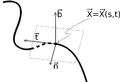
At ordinary point where , and , are bounded the first terms in r.h.s. of (80) dominate and the curve, locally, is a twisted cubic. Its projections on the osculating plane (spanned by and ), normal plane (spanned by and ) and rectifying plane (spanned by and ) are parabola (), cusp () and cubic () respectively (fig. 2, see e.g. [91]).

Characteristic feature of a curve (and a filament) in an ordinary point (i.e., outside the points of gradient catastrophe) is that it lies always on one side of positive direction of the normal and on one side of rectifying plane.
At the point of gradient catastrophe the behavior of a curve changes drastically. Indeed, when and (i.e. and ) become large, the r.h.s. of the formula (80) contains two parameters: small and large and . So, the second terms in and become relevant and different balance between and () lead to different regimes in behavior of a curve around the origin. For instance, parabola in the osculating plane may change sign or even convert into cubic curve (fig. 4) while in the normal plane it could be a plane curve and so on (fig. 3).


So, around the point of gradient catastrophe a filament oscillates from one side of the rectifying plane to another and back. Such oscillation is quite similar to that of airfoil (see e.g. [72]) and one can refer to these oscillations of a filament in the point of gradient catastrophe as a flutter.
Another peculiarity of the point of gradient catastrophe can be seen in the behavior of the focal curve associated with filaments. The focal curve (see e.g. [91]) is formed by the totality of centers of osculating spheres. Osculating sphere has a contact of third order with the curve in a points. Its center has coordinates
| (81) |
where is the position vector of a point on the curve. The radius of the osculating sphere is given by
| (82) |
For a set of regular points the corresponding piece of the focal curve is regular too and it lies on a finite distance from the original curve.
At the point of gradient catastrophe and, hence, the center of the osculating sphere as well as its radius blow up to infinity in the direction of the binormal vector (catastrophe direction, see figure 5).

So, the point of gradient catastrophe for the original curve at which both curvature and torsion are finite corresponds to a point of the focal curve at which the second focal curvature () becomes singular. We emphasize that even if our consideration for the original curve is purely local at the point of gradient catastrophe one observes a nonlocal effect of unbounded increase of the distance between a point on the original curve and the corresponding point on the associated focal curve.
We note that the blow-up of and for the focal curve happens also at the flattening points at which (for a discussion on the flattening points see e.g. [92]). It would be of interest to understand fully a difference between the flattening points on a curve and points with unbounded in pure geometrical terms. As an obvious difference one may observe that at the flattening point the projection of the curve on the osculating plane remains to be a parabola and the velocity and acceleration remain bounded too.
7 Elliptic umbilic and higher catastrophes
In order to understand better the phenomenon described above one should analyze in more detail the structure of the singularity and the regularizing mechanism for the gradient catastrophe. For the focusing NLS equation such an analysis based on the -expansion of the integrals of motions of the NLS/Toda equation has been performed in [52]. Here we will follow a different approach proposed recently in [93].
Thus, we consider a neighborhood of the gradient catastrophe point and denote the values of at this point by . Following the double scaling limit method (see e.g. [94]-[95]) we will look for solutions of the system (47) near the point of gradient catastrophe in the form
| (83) |
where and numbers should be fixed by further consideration. In our approach the function is the principal object for such an analysis. For the system (47)
| (84) |
where
| (85) |
For the solutions of the system (47) one has
| (86) |
and also, for , equation (50), i.e. . Furthermore differentiating EPD equation (42) with respect to , one has
| (87) |
Hence, at the point of gradient catastrophe , due to equation (50) and , one gets
| (88) |
where . So, at the expansion (83) for the function , the third order derivatives and are the only nonvanishing third order derivatives in the singular sector .
As a result, an expansion of the function near the point of gradient catastrophe is given by
| (89) |
Consequently
| (90) |
For generic point in the third term is smaller than the second one and the nontrivial balance of three terms in (90) is achieved if , i.e. .
Thus, near to the point of gradient catastrophe
| (91) |
where
| (92) |
and
| (93) |
Denoting , one has
| (94) |
where and are certain linear combinations of and . In Thom’s catastrophe theory language a function of this form is known as describing elliptic umbilic catastrophe [73].
The type of behavior of and near to the point of gradient catastrophe follows from (70) and (90). Indeed, near to the point , one has
| (95) |
Hence and
| (96) |
The elliptic umbilic singularity (94) and formula (96) describe generic point of gradient catastrophe which corresponds to the sector . For variable parameters , and other parameters describing the family of initial data, higher singularities corresponding to the singular sectors discussed in section 5 may appear.
For instance, if for some , , and then instead of the expansions (89) one has
| (97) |
So,
| (98) |
and, hence, in this case
| (99) |
Thus, at the sector one has
| (100) |
where
| (101) |
and as in the previous case (when ), while now .
Denoting , one gets
| (102) |
The last three terms reproduce the canonical form of a (nonsimple) unimodular parabolic singularity in terms of Arnold’s classification.
Near to the point of gradient catastrophe the behavior of is given by
| (103) |
Therefore and
| (104) |
In the sector generically one has and therefore
| (105) |
where
| (106) |
with and
| (107) |
Appearance of these singularities and particularly the time order of their appearance strongly depends on concrete structure and properties of vortex filament.
For nongeneric point of singular sector one might have a different behavior of function . For instance, for the singular sector in situation when
| (108) |
the third term in (89) of the order becomes relevant and the balance of order requires that . Hence, in such situation , and instead of the expression (90) one has
| (109) |
where
| (110) |
So, in the case (108) the variables and play a quite different role in contrast to the generic case (92), (93). Such type of behavior will be studied elsewhere.
8 Double scaling regularization. Painlevé I and other equations
At the point of gradient catastrophe the quasiclassical approximation ceases to be valid and contribution of the higher order derivatives terms in the governing equation becomes relevant. A standard way to deal with this problem is to begin with the full (dispersionfull) version of the governing equation (i.e. Da Rios system (4) or intrinsic version of equation (9)) and, then, performing an appropriate double scaling limit, calculate the required regularization terms. For the NLS equation (5) such an analysis has been performed in [52].
Here we will follow another approach discussed in [93, 71]. The basic idea is to incorporate higher order derivatives terms without any reference to the exact (dispersionfull) equation.
The first step is based on the observation (section 3) that governing equations describe critical points of the function . Thus, in order to incorporate derivatives of , it is quite natural to modify to in such a way that equation (40) is substituted by the Euler-Lagrange equations
| (111) |
for the functional .
Second point is to use the specific properties of the function . Namely, the real-valuedness of
| (112) |
and the fact that in the perturbations (see formulas (92), (106)) the contributions of and are separated. It is natural to look for the modifications of which preserve these properties. Thus, near the point of gradient catastrophe one has the following (omitting inessential terms in (91) and (92) and choosing )
| (113) |
where and are appropriate constants. Euler-Lagrange equations
| (114) |
implies that . So, one has the equation
| (115) |
This equation is converted into the classical Painlevé I equation
| (116) |
by the change of variables
| (117) |
with .
So, the regularized behavior at the point of the gradient catastrophe for the vortex filament dynamics is governed by the Painlevé I equation. The relevance of this equation for the NLS/Toda system near to the critical point has been first observed in a different way in [52]. The correspondence between the solution of equation (115) and those given by the formula (5.21) in [52] is (at ) , and
| (118) |
where , , and are defined in (2.19) and (2.22) of [52]. One also concludes that .
In the paper ([52]) it was conjectured that any generic solution of the NLS equation near to the critical point is described by the tritronqueé solution of the Painlevé I equation. Extension of this observation to our case allows us to formulate the
Conjecture 8.1.
Generic behavior of the vortex filament near the point of gradient catastrophe within the localized induction approximation is given by
| (119) |
where is the tritronqueé solution of the Painlevé I equation (116).
Such an approach can be extended also to the singular sectors . In these sectors the modified , for example, can be chosen in the following form
| (120) |
where are appropriate constants. The Euler-Lagrange equation readily implies that . So, the modified is given by
| (121) |
and the corresponding Euler-Lagrange equation for is
| (122) |
By the appropriate change of variables
| (123) |
one gets the equation
| (124) |
Eventual relation of these equations with appropriate limits of NLS hierarchy, higher Painlevé equations and other types of regularizations containing higher order derivatives will be considered in a separate paper.
Acknowledgements The authors are grateful to M. Bertola, B. Dubrovin and E. Ferapontov for useful discussions. This work has been partially supported by PRIN grant no 28002K9KXZ and by FAR 2009 (Sistemi dinamici Integrabili e Interazioni fra campi e particelle) of the University of Milano Bicocca.
References
- [1] Batchelor G.K. An introduction to fluid mechanics, Cambridge Univ. Press, Cambridge (1967)
- [2] Saffman P.G. Vortex dynamics, Cambridge Univ. Press, New York (1992)
- [3] Da Rios L.S. Sul moto d’un liquido indefinito con un filetto vorticoso (in Italian) Rend. Circ. Mat. Palermo 22 117-135 (1906)
- [4] Hama F.R. Localized induction concept on a curved vortex and motion of an elliptic vortex ring, Phys. Fluids 5 1156-1162 (1962)
- [5] Arms R.J. and Hama F.R. Localized induction concept on a curved vortex and motion of an elliptic vortex ring, Phys. Fluids 8 553-559 (1965)
- [6] Betchov R. On the curvature and torsion of an isolated vortex filament. J. Fluid. Mech. 22 471-479 (1965)
- [7] Ricca R.L. The contributions of Da Rios and Levi-Civita to asymptotic potential theory and vortex filament dynamics Fluid Dyn. Res. 18 245-268 (1996)
- [8] Hasimoto H. Soliton on a vortex filament J. Fluid. Mech. 51 477-485 (1972)
- [9] Zakharov V.E. and Shabat A.B. Exact theory of two-dimensional self-focusing and one-dimensional self-modulation of waves in nonlinear media ZETF 61 118 (1971); Sov. Phys. JTEP 34 62 (1972)
- [10] Lamb Jr. G.L. Solitons on moving space curves J. Math. Phys. 18 1654-1661 (1977)
- [11] Kida S. A vortex filament moving without change of form J. Fluid. Mech. 112 379-409 (1981)
- [12] Levi D. Sym A. and Wojcieckowski S. N-solitons on a vortex filament Phys. Lett. A 94 408 (1983)
- [13] Cieslinski J. Gragert P.K.H. and Sym A. Exact solution to localized-induction-approximation equation modeling smoke ring motion Phys. Rev. Lett. 57 1507-1510 (1986)
- [14] Fukumoto Y., J. Phys. Soc. Jap., 56, 4207-4209 (1987)
- [15] Langer J. and Perline R. Poisson geometry of the filament equation J. Nonlinear Sc. 1 71-93 (1991)
- [16] Klein K. and Majda A. Self-stretching of a perturbed vortex filament I Physica D 49 323 (1991); II, Physica D 53 267 (1991)
- [17] Nakayma K., Segur H. and Wadati M. Integrablity and the motion of curves Phys. Rev. Lett. 69, 2603-2606 (1992)
- [18] Ricca R. Physical interpretation of certain invariants for vortex filament motion under LIA Phys. Fliuds A 4 938-944 (1992)
- [19] Klein R., Majda A. J., McLaughlin R. M. Asymptotic equations for the stretching of vortex filaments in a background flow field. Phys. Fluids A 4 10, 2271–2281 (1992)
- [20] Langer J. and Perline R., Local geometric invariants of integrable evolution equations J. Math. Phys. 35, 1732–1737 (1994)
- [21] Nishiyama T. and Tani A. Solvability of the localized induction equation for vortex motion Comm. Math. Phys. 162 no. 3, 433–445 (1994)
- [22] Fukumoto Y., Miyajima M., The localized induction hierarchy and the Lund-Regge equation. J. Phys. A 29 no. 24, 8025–8034 (1996)
- [23] Kuznetsov E. A., Ruban V. P. Hamiltonian dynamics of vortex and magnetic lines in hydrodynamic type systems Phys. Rev. E (3) 61 no. 1 831–841 (2000)
- [24] Yasui Y. and Sasaki N. Differential geometry of the vortex filament equation J. Geom. Phys. 28 195-207 (1998)
- [25] Grinevich P. G. and Schmidt M. U. Closed curves in R3 and the nonlinear Schrödinger equation Proceedings of the Workshop on Nonlinearity Integrability and All That: Twenty Years after NEEDS ’79 (Gallipoli 1999) 139–145 World Sci. Publ. River Edge NJ 2000
- [26] Schief W. K. and Rogers C. Binormal motion of curves of constant curvature and torsion. Generation of soliton surfaces R. Soc. Lond. Proc. Ser. A Math. Phys. 455 3163-3188 (1999)
- [27] Ruban V. P. Applicability of the hodograph method for the problem of long-scale nonlinear dynamics of a thin vortex filament near a flat boundary Phys. Rev. E, 67 066301 (2003)
- [28] Gutierrez S. Rivas J. and Vega L. Formation of singularities and self-similar vortex motion under the localized induction approximation Commun. Partial Diff. Equations 28 927–968 (2003)
- [29] Holm D. D. and Stechmann S.N. Hasimoto Transformation and Vortex Soliton Motion Driven by Fluid Helicity arXiv:nlin/0409040
- [30] Konno K. and Kakukhata Kh A new type of stretched solutions, excited by initially stretched vortex filaments, of the local induction equation Theoret. and Math. Phys. 144 1181–1189 (2005)
- [31] Schief W. K. and Rogers C. The Da Rios system under a geometric constraint: the Gilbarg problem. J. Geom. Phys. 54 no. 3, 286–300 (2005)
- [32] Holm D. D., Nitsche M. and Putkaradze V. Euler-alpha and vortex blob regularization of vortex filament and vortex sheet motion. J. Fluid Mech. 555 149–176 (2006)
- [33] Calini A. and Ivey J. Finite-gap solutions of the vortex filament equation: isoperiodic deformations Nonlinear Sci. 17 527-567 (2007)
- [34] Onodera E. Generalized Hasimoto transform of one-dimensional dispersive flows into compact Riemann surfaces SIGMA 4 , Paper 044, 10 pp.(2008)
- [35] Banica V. and Vega L. On the stability of a singular vortex dynamics Commun. Math. Phys. 286 593-627 (2009)
- [36] Strong S.A. and Carr L.D. Generalized Local Induction Equation, Elliptic Asymptotics, and Simulating Superfluid Turbulence arXiv: 1102.2258
- [37] Moore D. W. and Saffman P. G. Vortex motion with axial flow Phil. Tans. Royal Soc. London Ser. A 272 403-429 (1972)
- [38] Callegari A. J. and Ting L. Motion of a curved vortex filament with decaying vortical core and axial velocity SIAM J. Appl. Math. 35 no. 1 148–175 (1978)
- [39] Leibovich S. and Ma H. Y. Soliton propagation on vortex cores and the Hasimoto soliton. Phys. Fluids 26 no. 11 3173–3179 (1983)
- [40] Maxworty T., Hopfinger E. J. and Redekopp L. G. Wave motions on vortex core J. Fluid Mech. 151 141-165 (1985)
- [41] Fukumoto Y. and Miyazaki T. Three-dimensional distortions of a vortex filament with axial velocity J. Fluid. Mech. 222 369-416 (1991)
- [42] Tani A. and Nishiyama T. Solvability of equations for motion of a vortex filament with or without axial flow. Publ. Res. Inst. Math. Sci. 33 no. 4 509–526 (1997)
- [43] Hirota R, Exact envelope-soliton solutions of a nonlinear wave equation J. Math. Phys. 14 805 (1973)
- [44] Forest M.G. and Lee J.E. Geometry and modulation theory for the periodic nonlinear Schroedinger equation in: IMA Volumes in Mathematics and its applications 2 36-69 Springer New York (1986)
- [45] El G.A. Gurevich A.V. Khodorovskii V.V. and Krylov A.L. Modulational instability and formation of a nonlinear oscillatory structure in a “focusing” medium Phys Lett. A 177 357-361 (1993)
- [46] Miller P.D. and Kamvissis S. On the semiclassical limit of the focusing nonlinear Schrödinger equation Phys Lett. A 247 75-86 (1998)
- [47] Bronski J.C. Spectral instability of the semiclassical Zakharov-Shabat eigenvalue problem. Advances in nonlinear mathematics and science Physica D 152-153 163-170 (2001)
- [48] Cai D. McLaughlin D.W. and McLaughlin K.T.R. The nonlinear Schrödinger equation as both a PDE and a dynamical system Handbook of dynamical systems 2 599–675 North-Holland Amsterdam (2002)
- [49] Kamvissis S. McLaughlin K.D.T.-R. and Miller, P.D. Semiclassical soliton ensembles for the focusing nonlinear Schrödinger equation in: Annals of Mathematics Studies 154 Princeton University Press Princeton NJ (2003)
- [50] Ercolani N. M., Jin S., Levermore C. D, and MacEvoy W. D. Jr., The zero-dispersion limit for the odd flows in the focusing Zakharov-Shabat hierarchy. Int. Math. Res. Not. 47 2529–2564 (2003)
- [51] Tovbis A., Venakides S. and Zhou X. On semiclassical (zero dispersion limit) solutions of the focusing nonlinear Schrödinger equation Commun. Pure Appl. Math. 57 877-985 (2004)
- [52] Dubrovin B. Grava T. and Klein C. On universality of critical behavior in the focusing nonlinear Schrödinger equation, elliptic umbilic catastrophe and the tritronquée solution to the Painlevé-I equation J. Nonlinear Sci. 19 57–94 (2009)
- [53] DiFranco J. C. and Miller P. D. The semiclassical modified nonlinear Schrödinger equation. I. Modulation theory and spectral analysis. Phys. D 237 no. 7, 947–997 (2008)
- [54] Tovbis A and Venakides S. Semiclassical limit of the scattering transform for the focusing Nonlinear Schrödinger Equation arXiv:0903.2648
- [55] Tovbis A and Venakides S., Nonlinear steepest descent asymptotics for semiclassical limit of integrable systems: continuation in the parameter space. Comm. Math. Phys. 295 no. 1 139–160 (2010)
- [56] Bertola M. and Tovbis A. Universality for the focusing nonlinear Schroedinger equation at the gradient catastrophe point: Rational breathers and poles of the tritronquée solution to Painlevé I arXiv:1004.1828
- [57] Bertola M. and Tovbis A. Universality in the profile of the semiclassical limit solutions to the focusing nonlinear Schrödinger equation at the first breaking curve Int. Math. Res. Not. IMRN 11 2119–2167 (2010)
- [58] Jenkins R. and McLaughlin K. D. T.-D., The semiclassical limit of focusing NLS for a family of non-analytic initial data arXiv:1106.1699 (2011)
- [59] Zakharov V.E. Benney equations and quasiclassical approximation in the inverse problem method Func. Anal. Appl. 14 89-98 (1980)
- [60] Boyer C. P. and Finley J. D., III Killing vectors in self-dual, Euclidean Einstein spaces. J. Math. Phys. 23 no. 6, 1126–1130 (1982)
- [61] Kodama Y. Solutions of the dispersionless Toda equation. Phys. Lett. A 147 no. 8-9 477–482 (1990)
- [62] Takasaki K. and Takebe T. SDiff(2) Toda equation—hierarchy, tau function, and symmetries. Lett. Math. Phys. 23 no. 3, 205–214 (1991)
- [63] Takasaki K. and Takebe T.Integrable hierarchies and dispersionless limit. Rev. Math. Phys. 7 no. 5, 743–808 (1995)
- [64] Gerasimov A., Marshakov A., Mironov A., Morozov A. and Orlov A. Matrix models of two-dimensional gravity and Toda theory. Nuclear Phys. B 357 no. 2-3, 565–618 (1991)
- [65] Wiegmann P. B. and Zabrodin A. Conformal maps and integrable hierarchies. Comm. Math. Phys. 213 no. 3 523–538 (2000)
- [66] Krichever I., Mineev-Weinstein M., Wiegmann P. and Zabrodin A. Laplacian growth and Whitham equations of soliton theory. Phys. D 198 no. 1-2, 1–28 (2004)
- [67] Konopelchenko B., Martínez Alonso L. and Medina E. On the singular sector of the Hermitian random matrix model in the large N limit. Phys. Lett. A 375 no. 5 867–872 (2011)
- [68] Lavrentʹev M. A general problem of the theory of quasi-conformal representation of plane regions. (Russian) Mat. Sbornik N.S. 21 (63) 285–320 (1947)
- [69] Ahlfors L. V., Lectures on quasiconformal mappings. Van Nostrand Mathematical Studies, No. 10 D. Van Nostrand Co., Inc., Toronto, Ont.-New York-London (1966)
- [70] Bojarski B., Quasiconformal mappings and general structural properties of systems of non linear equations elliptic in the sense of Lavrentʹev. Symposia Mathematica 18 485–499 (1976)
- [71] Konopelchenko B. G. and Ortenzi G. Gradient catastrophe and flutter in vortex filament dynamics. J. Phys. A 44 no. 43, 432001, 12 pp (2011)
- [72] Milne-Thompson L.M., Theoretical Hydrodynamics McMillan & co. (1960)
- [73] Thom R., Structural stability and morphogenesis. An outline of a general theory of models Addison-Wesley Publishing Company Redwood City CA (1989)
- [74] Arnol’d V.I. Guseĭn-Zade S.M. and Varchenko A.N. Singularities of differentiable maps. Vol. I. The classification of critical points, caustics and wave fronts Monographs in Mathematics 82 Birkhäuser Boston Inc. Boston MA (1985)
- [75] Weinstein A. The singular solutions and the Cauchy problem for generalized Tricomi equations Commun. Pure Appl. Math. 7 105-116 (1954)
- [76] Roždestvenskiĭ B. L. and Janenko N. N., Systems of quasilinear equations and their applications to gas dynamics Transl. Math. Mon. 55 AMS Providence RI (1983)
- [77] Landau L. D. and Lifshitz E. M. Fluid mechanics Course of Theoretical Physics, Vol. 6 Pergamon Press Ltd (1959)
- [78] Gurevich A.V. and Shvartsburg A.B. Exact solutions of nonlinear geometrical optics equations JETP , 58 2012-2022 (1970)
- [79] Shvartsburg A.B. Nonlinear geometric optics in nonlinear wave theory. Nauka Moscow (1976)
- [80] Kudashev V. R. and Suleimanov B.I. Characteristic features of some typical spontaneous intensity collapse processes in unstable media. JETP letters 62 358-363 (1995)
- [81] Garifullin R. N. and Suleimanov B. I. From weak discontinuities to nondissipative shock waves. JETP 110 133-146 (2010)
- [82] Darboux G. Leçons sur la théorie générale des surfaces II Gauthier Villars (1915)
- [83] Tsarëv S. P. The geometry of Hamiltonian systems of hydrodynamic type. The generalized hodograph method. (Russian) Izv. Akad. Nauk SSSR Ser. Mat. 54 no. 5 1048–1068 (1990); translation in Math. USSR-Izv. 37 no. 2 397–419 (1991)
- [84] Kudashev V. R. and Sharapov S. E. Hydrodynamic symmetries for the Whitham equations for the nonlinear Schrödinger equation (NSE). Phys. Lett. A 154 no. 9, 445–448 (1991); Inheritance of symmetries in the Whitham averaging of the Korteweg-de Vries equation, and hydrodynamic symmetries of the Whitham equations. Theoret. and Math. Phys. 87 , no. 1, 358–363 (1991)
- [85] Gurevich A.V., Krylov A.L., El G.A. Breaking of a Riemann wave in dispersive hydrodynamics. Jetp Letters 54 104-109 (1991)
- [86] Tian F. R., Oscillations of the zero dispersion limit of the Korteweg-de Vries equation. Comm. Pure Appl. Math. 46 no. 8 1093–1129 (1993)
- [87] Pavlov M.V., Integrable hydrodynamic chains. J. Math. Phys. 44 no. 9 4134-4156 (2003)
- [88] Konopelchenko B. Martínez Alonso L. and Medina E. Hodograph solutions of the dispersionless coupled KdV hierarchies, critical points and the Euler-Poisson-Darboux equation J. Phys. A: Math. Theor. 43 434023 (2010)
- [89] Konopelchenko B. Martínez Alonso L. and Medina E. Singular sectors of the 1-layer Benney and dToda systems and their interrelations Theor. Math. Phys. 168 (1), 963-973 (2011)
- [90] Beltrami E. Sulla teoria delle funzioni potenziali simmetriche Mem R. Accad. Sci. Bologna 2 461-505 (1880); Opere Mat. 3 349-382 (1911)
- [91] Eisenhart L.P., An introduction to differential geometry Princeton Univ. Press princeton (1947)
- [92] Uribe-Vargas R. On the stability of bifurcation diagrams of vanishing flattening points. (Russian) Funktsional. Anal. i Prilozhen. 37 no. 3, 88–94 (2003); translation in Funct. Anal. Appl. 37 no. 3, 236–240 (2003)
- [93] Konopelchenko B. and Martínez Alonso L., Catastrophes, double scaling regularization and integrable systems (in preparation)
- [94] Di Francesco P. Ginsparg P. and Zinn-Justin Z. 2D gravity and random matrices Phys. Rep. bf 254 2 (1995)
- [95] Martínez Alonso L. and Medina E. The double scaling limit method in the Toda hierarchy J. Phys. A: Math. Theor. 41 335202 (2008)